1. Introduction
Rainfall is very important for the hydrological cycle with a major influence on the environment and agricultural productivity worldwide (Ayehu et al. 2018). It has a significant effect on rainfed agriculture, hydropower, socioeconomic development and human activity (Degefu & Bewket 2023).The schedule of agricultural activities, such as land preparation, crop selection and planting, and post harvesting activities for Africa is rainfall dependent (Alaminie et al. 2021).Hence, the variability and change in the onset, cessation, and duration of rainy season are the major socio economic and developmental challenges that lead to food insecurity and poverty in Africa (Kwawuvi et al. 2022).
Ethiopia’s climate is characterized by significant seasonal and regional variations in the volume and distribution of rainfall (Zeleke et al. 2023). Because of this, the majority of the country’s highlands in the center and east have a coefficient of variability (CV) of less than 30% values in millimeters of rainfall, while the lowlands in the north, north east, and south east have a CV of 70% or more (Zeleke et al. 2023). In general, the country’s rainfall coefficient of variation values ranged from 10% to 70%. Rainfall is unpredict Table, because of its both spatial and temporal unpredictability, and this variance in the distribution of rainfall over space and time generates major hydrological issues (Mensah et al. 2016).The threat posed by climate variability and change has grown, endangering national food security, sustainable development but also human existence as a whole (Taye et al. 2013).Ethiopia’s topography is composed of massive highlands, complex mountains, and dissected plateaus divided by a great rift valley generally running south east to north east. This great terrain diversity in the country determines the wide variations in climate, soil, natural vegetation, and settlement patterns ( Degefu et al. 2017)
Owning to its tropical location, Ethiopia is subject to a wide range of weather systems, from large-scale ENSO-related phenomena to meso-scale phenomena such as thunderstorms. The inter-tropical convergence zone (ITCZ) is the main rain-bearing system during the main rainy season, which runs from June to September (Degefu et al. 2022). The inter-tropical Convergence Zone (ITCZ) is the area in which the north east and south east trade winds meet (Degefu et al.2022). Conversely, during the small rainy season Belg (February to May), the east ward-moving mid-latitude troughs facilitate the interaction between mid-latitude cold air and tropical warm air, creating unstable conditions for the moisture that enters Ethiopia from the Arabian Sea (Evangelista et al. 2013).
For planting and other agricultural activities during the main rainy season (Kiremt), it is also crucial that there is a relationship between the onset date, cessation dates and the length of the season. Long-term daily rainfall data for 58 locations in West African climate zones were analyzed by Lotfie et al. (2018).The results of this study demonstrated a strong correlation between the length of the growing season and the arrival of rainfall. They found that the length of the growing season was more dependent on the start of the rainy season than on its cessation. Planting (sowing) dates, crop development, yield, and food production are affected by the misinformation of the onset, cessation, and length of the growing season (Amekudzi et al. 2015; Mensah et al. 2016; Owusu et al. 2009). In responsive farming, a less hazardous planting date, planting technique, or sowing of less hazardous crop types or varieties require accurate rainfall and characteristic prediction, particularly the onset date (Mensah et al. 2016).
A wide area of approximately 15 million hectares in the Amhara region is available for crop cultivation, which is dependent entirely on rainfall (Taye et al. 2013).The western part of the region is more favorable for crop cultivation, but has mono-modal rainfall pattern (only the Kiremt rainfall benefiting area).These regions span several climate zones with varying amounts of rainfall and varying start and end dates. The amount and distribution of rainfall vary, and this affects both the annual planted areas and crop yields (Eldin et al. 2015).
Over the Western Amhara Region, there are limited studies on past and future rainfall characteristics. In fact, analysis of the past and prediction of future daily to seasonal climate can help to minimize the possible occurrence of climate change in order to reduce impacts on social welfare and ecosystems (Ayalew et al. 2012). Therefore, the novelty of this study is understanding the characteristics of the past and future rainfall situations for preparing agricultural plans that will help increase crop productivity and other socio-economic development by buffering situations where increased stresses are likely to occur.
2. Materials and Methods
2.1. Study Area
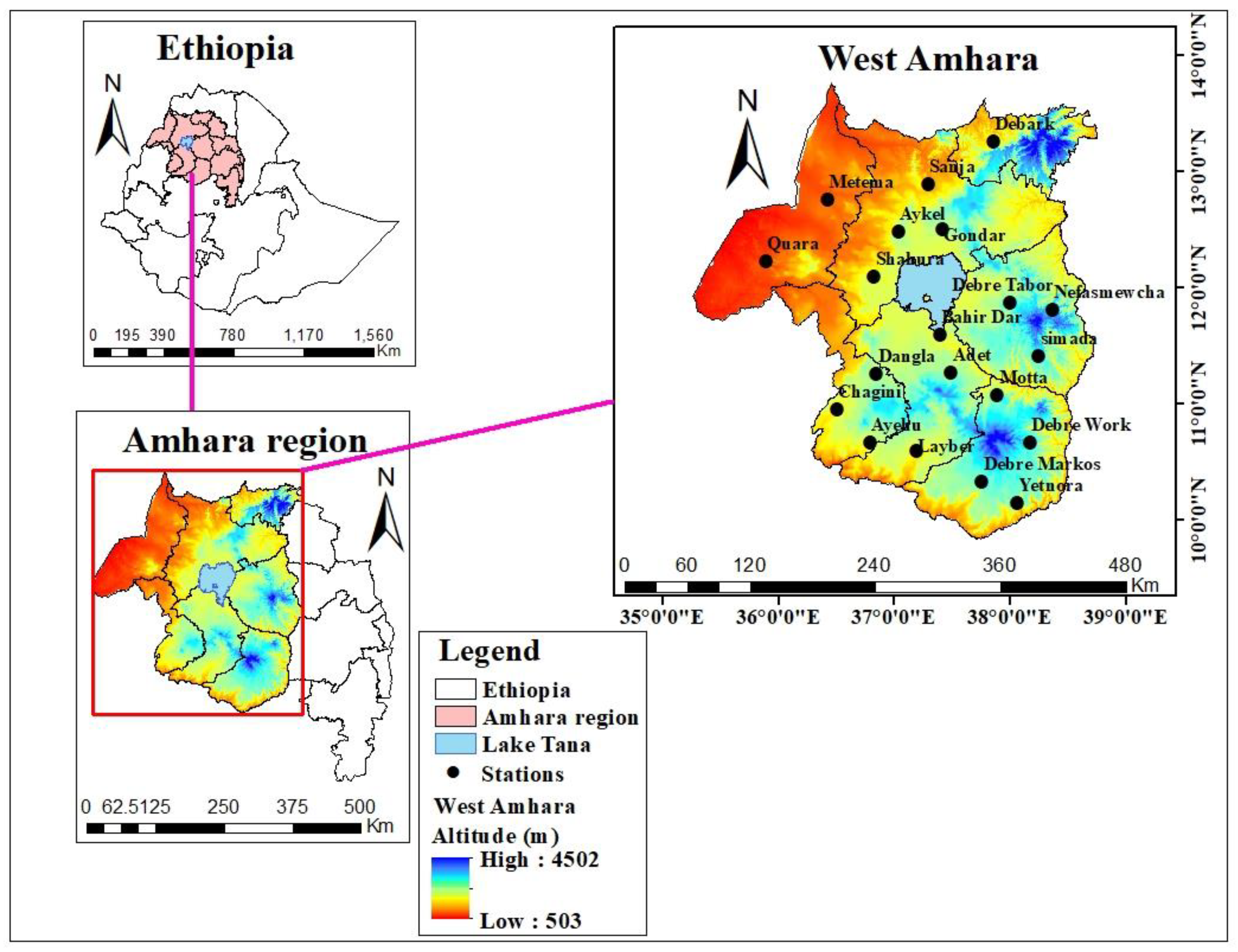
The Amhara Region is located between latitudes of 8°45’N and 13°45’ N and longitudes of 35° 46’ E and 40° 25’ E, whereas the western Amhara region is located between latitudes of 9°50’ N and 13°45’N and longitudes of 35° 16’ and 38° 44’ E (
Figure 1). The total area of the Amhara region is estimated to be 156,960 km
2 (Taye
et al. 2013).Based on altitude, mean annual rainfall, and mean annual temperature, the climate of western Amhara region was divided into four climatic zone categories. The
Kola/tropical (hot zone) covers 31% of the region, which is located below 1500 m.a.s.l. Whereas,
Woyina Dega/sub-tropical (warm zone), covers 44%, which is between 1500 - 2500 meter above sea level. The remaining, Dega/temperate (cold zone) covered 24%, which is located between 2500 -3200 m.a.s.l., and approximately 1% is covered by
wurch/alpine ( kur zone) (Taye
et al. 2013).
Western Amhara experienced heavy rainfall during June, July, August, and September months. This season contributes 77.05% of the mean annual rainfall of western Amhara. The mean annual rainfall of western Amhara was 1054.2 mm. The mean annual temperature of the study area is 18.0 °C. But in the valleys and marginal areas, the temperature exceeds 27 °C (Taye et al. 2013).
Agriculture continues to be the predominant economic industry in this area. In terms of structure, it contributes, on average, 55.8% of the regional GDP, and 88.7% of the population makes their living from farming and related industries (Taye et al. 2013). It is the main supplier of food, raw materials, and revenue from exports to close industries. The area is home to a variety of flora and fauna species owning to its unique agro-ecology.
The geographical features of the Amhara region show a range of elevations, from over 4600 meters above sea level (m.a.s.l.) in the north west to 700 m above sea level (m.a.s.l.) in the eastern edge. According to the Salinger and Stryker, (2001) assessment report, the majority of the Amhara region is on highland plateaus, which are defined by craggy mountains, hills, plateaus, valleys, and gorges. As a result, the landscape of the area is diverse, with eroded landforms in the north, virtually flat plateaus and mountains in the center, and high fault slopes and nearby lowland plains in the east. A level plain that extends into the Sudan lowlands constitutes the majority of the western region. Aproximately half of the region’s total area is potentially arable for agricultural production. According to Bazezew (2012),60% of the entire area is currently used for agriculture and grazing (30% each), 17% is covered in woods, woodlands, and shrub lands, 4% is water, 3% is inhabited by communities, and 16% is wasteland.
2.2. Data Types and Sources
2.2.1. Ground-Based (Observed) Rainfall Data
To characterize past rainfall during the main rainy season (Kiremt ) over western Amhara, sample meteorological stations were purposively selected based on the availability of daily rainfall data and the fair distribution of the station for the period 1991-2020.Hence, based on their relative quality and long timeseries, 20 meteorological stations were selected. The 30-year records of daily rainfall data was collected from the Ethiopian Meteorology Institute (EMI) of Ethiopia (
Figure 1)
Quality Control was the primary task before any further analysis. Prior to analysis, the observed rainfall data of all station was plotted against time DOY (day of the year) format and subjected to visual examination for the presence of discontinuities and special codes for missing values (Tegegn, 2015). The primary issues that meteorological analysts frequently face is missing data (Taye et al. 2013). The missing data were filled and evaluated using the INSTAT Markov chain simulation model (Stern et al. 2006). This is because the first order does not exaggerate the result and moreover, it provides an accurate model estimate as explained by Stern et al. (2006). Outlier detection of the daily observed rainfall data for the period 1991–2020 was done. The quartile outlier detection technique using climate data tools (CDT) (Dinku et al. 2022). The common Standard Normal Homogeneity Test (SNHT) was used to check daily observed rainfall data using the Climate Data Tool (CDT) packages (Dinku et al. 2022).
2.2.2. CMIP6 GCMs Data
To select Inter-comparison Project phase 6 Global Climate Models(CMIP6GCMs) for future rainfall characteristics analysis first evaluation of CMIP6 GCMs using observed gauge and CMIP6 GCMs historical was made. Among the observed data for 1991-2020 collected for 20 stations, for performance evaluation purpouse, the rainfall data of each station for the period 1995-2014 was organized. Similarly Site-specific historical daily rainfall data were downloaded from CMIP6 GCMs for rainfall for the period 1995-2014. Daily GCM data of those GCMs obtained from the Earth System Grid Federation (ESGF) database at
https://esgf node.llnl.gov/projects/cmip6/. Numerous CMIP6 GCMs can project future climates under different shared socio-economic pathways (SSP) (Gashaw
et al. 2024). However, the performance of the GCMs differs from region to region. Hence a performance evaluation is crucial before use in any application. The selection of the GCMs for performance evaluation was based on the availability of daily data and their best performance in different parts of Ethiopia (Gashaw
et al. 2024),East Africa (Gebrechorkos
et al. 2023) ,and else where in the world (Iqbal
et al. 2021).The models were also selected based on their wider applications in earlier versions (CMIP5) in different parts of Ethiopia (Worku
et al. 2020).For example, the inclusion of BCC-CSM2-MR was based on the best performance for simulating rainfall in the Upper Blue Nile Basin of Ethiopia (Alaminie
et al. 2021).EC-Earth3 and EC-Earth3-Veg were selected because they demonstrated the best performance in mainland southeast Asia (Iqbal
et al. 2021).The inclusion of MPI-ESM1-2-LR and GFDL-ESM4 for evaluation was because of their relatively good performance in representing the total monthly rainfall over the Bale eco region in Southern Ethiopia (Gashaw
et al. 2024). A study conducted over the Upper Blue Nile basin, in Ethiopia, recommended BCC-CSM2-MR for simulation of annual, Kiremt, and Belg rainfall season, whereas MRI-ESM2-0 for bega season rainfall simulation (Mohammed, 2024).GFDL-ESM4 was selected as recommended by Berhanu
et al.(2023) for monthly and seasonal rainfall simulations, after evaluating the performance of 37 CMIP6 GCMs. A study by Omay
et al.( 2023), recommended that BCC-CSM2-MR,and GFDL-ESM4 be selected, as these are recommended for seasonal rainfall simulation of East Africa after validating 23 CMIP6 GCMs with observed .MRI-ESM2-0 was recommended for Nigeria among 13 CMIP6 GCMs evaluation (Shiru & Chung, 2021).A study by Lebeza
et al.(2024) evaluated seven CMIP6 GCMs models and recommended Ec-Earth3,BCC-CSM2-MR,and BCC-CSM2-MR for simulation of daily,monthly, and annual rainfall over the Lake Tana sub-basin, Ethiopia respectively. Selected CMIP6 GCMs for this study are described in
Table 1.
2.3. Methods of Analysis
2.3. Performance Evaluation of CMIP6GCMs
Performance evaluations of the CMIP6 models in this study were undertaken after extracting the daily data of the five CMIP6 GCMs (
Table 3) for the 20 meteorological stations in the study area (Appendix Table 1) for the period 1995-2014. The station (point) data and each CMIP6 GCMs data were the areal averages for the Western Amhara scale, which were evaluated by comparing historical CMIP6 GCMs against observed rainfall data at daily, monthly ,and seasonal timescales separately. The performance of CMIP6 models under different Shared Socio-economic Pathways (SSPs) were evaluated in simulating future rainfall characteristics in the Western Amhara region based on efficiency criteria found under “hydroGOF” R package (Gashaw
et al. 2024). Numerous performance efficiency criteria exist for model evaluation (Gashaw
et al. 2024).However, most authors prefer to use performance efficiency criteria, including the root-mean square errors (RMSE), percentage of bias (PBIAS),and Pearson correlation coefficient (r) (Alaminie
et al.,2021; Gashaw
et al. 2024). The RMSE measures the average magnitude of the deviation of rainfall products from the ground based observed data (Equation 1). A smaller RMSE value indicated that rainfall products were closer to the observed rainfall data. The optimum value of RMSE is 0 (Ageet
et al. 2022). The PBIAS measures the average tendency of rainfall products data to be larger or smaller than the observed data. Percent bias (PBIAS) is a statistical metric that spans from -∞ to ∞, with an ideal value of zero. The low magnitude of the PBIAS suggests that the rainfall products accurately estimate the observed data. Negative values of PBIAS indicate a bias of overestimation in the rainfall products, whereas, positive values of PBIAS indicate a bias of underestimation in the rainfall products when compared to the observed data (Gupta
et al.1999). Rainfall products are said to be a reliable rainfall measurement sources where PBIAS value ranging between -10% and 10% (Dangol
et al. 2022). PBIAS can be calculated using (Equation 2). The correlation coefficient (r) was used to measure the goodness of fit and linear association between variables, in this case the linear association between the observed rainfall and rainfall product data (Equation 3). The values of r range from -1 to 1, with r = 0 indicating no linear relationship, and r = -1 or 1 indicating a perfect negative or positive score (Dinku
et al. 2018; Ageet
et al. 2022;Aniley
et al. 2023).
observed rainfall total at a gauge station,
is the mean of observed rainfall total at gauging station, S is rainfall total for CMIP6 GCMs rainfall product,
is the mean of CMIP6 GCMs rainfall total, N is the number of data pairs compared and r is Pearson’s correlation coefficient. The overall ranking of the five GCMs considering all statistical metrics (i.e., r, RMSE, and PBIAS) were undertaken following the Comprehensive Rating Index (CRI) method using Equation (Equation 4).
Where n is the number of statistical performance measures used in this study for evaluating the models (5), m is the number CMIP6 GCMs that are evaluated in the study (
Table 1), and Ranki is the rank of the CMIP6 GCMs for each performance measures, which ranges from 1 to 5 for best and low performing models, respectively. The closer the values of CRI to 1 indicates the better performance of the model (Gashaw
et al. 2024).
Bias corrections of the global dataset were performed using Distribution Mapping (DM) technique. Distribution Mapping (DM),which is available in the Climate Model data for hydrologic modeling (CMhyd) tool (Gashaw et al. 2024),is used for bias correction of best performing GCMs projections under different climate change scenarios. The selection of DM for bias correction of GCMs for rainfall was based on the suggestion of Worku et al.(2020), who compared several bias-correction techniques available in CMhyd in the Jemma sub-basin, Upper Blue Nile Basin of Ethiopia and suggested the application of DM for bias correction of rainfall and temperature products. Another study in the Awash Basin of Ethiopia also found that DM is suitable for the bias correction of climate models for temperature (Tadese et al. 2020). This study bias corrected the best performing CMIP6 GCMs (top three ranked) after extracting the data for each stations, hence bias correction was performed by providing the daily observed historical (1995–2014), raw GCMs historical (1995–2014) and future raw GCMs (2021–2100) data of each station in text file. In this study, the analysis of future climate for the near future (2021–2050), mid-century (2051–2080) and late-century (2081–2100) periods (Belazreg et al. 2023) was conducted at SSP2-4.5, SSP3-7.0 and SSP5-8.5 climate change scenarios for the Western Amhara level. Scenarios SSP2-4.5, SSP3-7.0 and SSP5- 8.5 scenarios are representing medium-forcing, medium to high forcing and high-end-forcing pathways, respectively. The main reason why this study performed the future climate change analysis in these scenarios is that three of them are possible climate change trajectories. On the other hand, the one that is not considered in this study (i.e., SSP1-2.6, representing the low climate forcing pathway)is unlikely to occur considering the current global actions undertaken to mitigate climate change based on the Paris Agreement. Therfore, future climate change analysis and bias corrections of global dataset were performed mainly for SSP2-4.5, SSP3-7.0 , and SSP5-8.5 climate change scenarios (Gashaw et al. 2024).
2.3.2. Determination of the Past Rainfall Characteristics
The quality-controlled rainfall data were organized used in excel 2010 spread sheet following the days of the year (DOY) entry format, and the daily rainfall data was subjected for detailed analysis using sequences of statistical packages. The appropriate OD, CD, and LGP was calculated and simulated by using the CDT tool (Dinku
et al. 2022). The onset date was calculated based on the following criteria , the day that recorded 20mm of rainfall over five consecutive days without being followed by a dry spell longer than seven days within 21 days of planting day and with at least three rainy days on which threshold for rainy days (> =0.85mm) (Dinku
et al. 2022).This was done to capture both the early start and the late start, and the condition that there should be no 7-day dry period is to ensure that there is no false start (Dinku
et al., 2022). The end of the growing season is the first occasion when the water balance drops to zero after the end of rain (Zeleke
et al. 2023).In this study the end of the rainy season was calculated using the CDT tool with the criterion that, the water balance drops below 5mm for a period of three days (Dinku
et al. 2022).The length of the growing season (LGP) for the main rainy season was determined as the number of days between the rainfall onset and cessation dates using Equation (5).
Trend analysis: After investigating /determining the OD, CD, LGP of the kiremt season using CDT tool, for the study area and for study time period (past and future) the timeseries pattern was analyzed by using Sen’s slope estimator and modified Mann-Kendal test (non-parametric trend test) using R-statistical Software at 5% significance level. The Mk trend test is the most suitable and favorable non-parametric test for identifying trends in timeseries climate data. This method is less influenced by missing values and uneven distribution and is less sensitive to outliers, because it considers the ranks of observations rather than their actual numbers (Belay et al. 2019).
The S-statistic was applied to check for an increasing, decreasing or no-change trend in the OD, CD, and LGP data series in each of the selected meteorological station data in the MK t- test statistic, which is given as follows:
The values Xj and Xk in Equation (6) are the measurements corresponding to times j and k, and n is the number of events. To estimate the variance of S: -
In Equation (7), n: number of observations; m: number of data pairs in the series; ti : number of ti’s at the timestep i (Silva 2017; Tadese
et al. 2019). Hamed and Ramachandra Rao (Hamed & Ramachandra Rao 1998) proposed a modified version of the MK test (MMK), which is a better alternative than the original MK test for detecting trends in time series exhibiting autocorrelation, a common characteristic in hydrological time series. The difference is in the formula used to calculate the variance for the MMK test:
where Var(S)* is the modified variance. With r R k corresponding to the lag-k autocorrelation coefficient of the ranks of the data, the correction factor n/n* is:
To determine the significance of the trend, both MMK and MK follow what is presented in Equation (10):
Trend analysis employs the Theil–Sen slope estimator (SS), a non-parametric metric that approximates the magnitude (Arrieta-Castro
et al. 2020). This metric is determined by the slopes of the lines (Qi) connecting the data pairs (N), with their values obtained through the following Equation:
Finally, the arrangement of the Q values in ascending order allows for the computation of the median using the Equation:
The trend of OD, CD, LGP, and kiremt season rainfall total for all sample stations and study time periods were easily calculated using R statistical package.
Variability analysis: The coefficient of variation (CV) is a relative measure of variability, that displays standard deviation relative to its mean (Morales-Acuña
et al. 2021). As a result, the coefficient of variation (CV), was used to determine the variability of the Western Amhara region OD, CD, LGP, and seasonal rainfall total for the past (1991-2020) using Equation (13).
Where: CV (%) is the coefficient of variation of OD,CD, LGP, and kiremt season rainfall for sample station, S is the standard deviation of OD, CD, LGP, and kiremt season for stations,µ is the mean of OD,CD, LGP, and kiremt season for stations during 1991-2020 time periods. The CV (%) can be interpreted as follows (Morales-Acuña et al. 2021).
When 0≤CV(%) <20, there is low variability between the given data of the given time scale.
When 20≤CV(%) <30, moderate variability was observed between the given data for the given time scale.
When CV(%) ≥30, there is high variability between the given data of the given time scale. Because of this, the magnitude of CV (%) of selected stations and regional scale were compared.
The Standardized Anomaly Index ( SAI) is a measure of variability, used to detect the variability and nature of the trend (Asfaw
et al. 2018). It was determined using Equation (14).
Where, Z is number of standard deviations of the observation deviated from the normal, x is an observed rainfall value and is mean rainfall and SD is the standard deviation. This statistic enables us to determine the dry (negative values) and wet (positive values) years in the observation. The rainfall anomaly value less than -1.65 is considered extremely drought, whereas a rainfall anomaly index greater than 1.65 considered to be extremely wet. The total Kiremt rainfall for the past (1991-2020) were calculated and identified as wet and dry years.
The PCI is used to examine the variability (heterogeneity pattern) of rainfall at different scales (annual or seasonal). The PCI value can help to identify periods of high rainfall that may lead to flooding as well as dry spells that can contribute to drought conditions. The PCI values were computed, as described by Oliver (1980) and modified by De Luis
et al. (2011). PCI can be calculated using Equation (15).
where: PCI is the precipitation concentration of the Kiremt season, and Pi is the rainfall amount of the ith month. According to Oliver (1980), PCI values less than 10 indicate a uniform monthly distribution of rainfall (low precipitation concentration), values between 11 and 15 denote moderate concentrations, values from 16 to 20 indicate high concentration, and values of 21 and above indicate very high concentrations (Asfaw et al. 2018).
Analysis of rainfall total: In a Box and whisker plots, the box represents the middle 50% of the whole data set, while whiskers represent the magnitude of the spread of the rest of the data set about the median or mean (Stern et al. 2006).The minimum, maximum, and mean daily rainfall total were summarized using a Box and Whiskers plot using the CDT tool (Dinku et al. 2022). The monthly and seasonal rainfall total were spatialy interpolated in ArcGIS software using the inverse distance weight interpolation technique for the past (1991-2020).
2.3.3. Determination of Future Rainfall Characteristics
For determination of future rainfall characteristics, the ensemble mean of the top three best performing CMIP6 GCMs were used for daily, monthly, and seasonal temporal scales, and each rainfall characteristics was analyzed by dividing the future time period as 2021-2050,2051-2080, and 2081-2100 for each SSPs for the Western Amhara region.The future rainfall characteristics (OD,CD,LGP, rainfall amount) variability ( using standard deviation, coefficient of variation, standardized anomaly),trend analysis (using the Mankendal trend test and Sen’s slope estimator) ,and daily rainfall total (using Box and Whiskers plot) were analyzed and interpreted in a manner similar to past rainfall analysis using the methodology described under sub-heading (2.3.2). More over, the departure of the future (2021-2100) monthly and seasonal rainfall totals under different SSPs from the past (1991-2020) were summarized in tabular form as Gashaw et al.(2024), also following a similar approach to the Bale Eco region in Southern Ethiopia.
3. Results and Discussions
3.1. Analysis of the Past Rainfall Characterstics
3.1.1. Analysis the Onset of the Main Rainy Season
The mean onset dae of Western Amhara for the main rainy season is shown in
Table 2 and Appendix Figure 1.In the region, the earliest and latest onset date for the period 1991 to 2020 was 124 DOY(3-May) and 164 DOY(16-June) respectively.The mean onset date ranged from 136 DOY(15-May) at Ayehu station to 159 DOY(7-June) at Simada and Nefas Mewucha stations. But the mean onset date of Western Amhara region was 138 DOY(17-May) for the specified study time period. A study by Ayalew et al. (2012) reported ,167 DOY (15-June) as the mean date of onset for Kiremt rainfall in the Amhara National Regional State. The standard deviation of onset date ranged from 10 days at Chagni to 24 days at Webre Work with region based standard deviation onset date of 14 days. On the other hand, the coefficient of variation varies from 7% at Chagni to 15% at Motta, Nefas Mewucha, and Debre Work stations, which is less variable. The overall coefficient of variation for the onset date in the region was 10%. A study by Wasihun
et al.(2017) showed that, the coefficient of variation of the onset date, cessation date, and length of growing period for the study time period 1988-2017 were 23%,7%,and 16% respectively. Overall, the start of the rainy season varied from place to place, and earlier onset dates were recorded in the Western part of the study area (Chagni),thanin the eastern part of the region (Simada and Nefas Mewucha).The result conveyed that, the start of the rainy season becomes latter as we go from western to Eastern of the study region. Previous study by Taye
et al.(2013) also noted, the variability of onset date among stations. According to Taye
et al.(2013) ,on average the
Kiremt rainfall at Bahir Dar, Motta, Debre Markos and Dangla stations began at 153 DOY (01-June),151DOY (30-May),144 DOY (23-May), and 132 DOY (11-May) respectively, and Zeleke
et al.(2023), over North West Ethiopia for the period 1987 to 2017 also showed that, the rainy season begins between 129 DOY (08-May) and 155 DOY (03-June).
Station wise and regional onset date trend for the period 1991-2020 was given in
Table 3.The result showed a decreasing trend of onset date for most of stations and regional level, except at Chagni, Simada, and Quara stations, Onset date showed decreasing trend means, the rainy season starts earlier from year to year. But the trend is statistically significant at 95% confidence level only at Ayikel and Debre Work stations with Sen’s slope estimator of 0.40 day/year and 1.0 day/year respectively. A study by Wasihun
et al.(2017) also showed that, increasing and significant onset date at 95% confidence level with Sen’s slope estimator of 0.16 day/year for the period 1988-2012 over Gelemso, West Harerghe.
Table 3.
Station wise and regional trend analysis of onset date for the period 1991-2020.
Table 3.
Station wise and regional trend analysis of onset date for the period 1991-2020.
| Station |
Z-Value |
Sen’s slope |
S |
Var(S) |
P-value |
Tau |
| Chagini |
0.27 |
0.00 |
16 |
3119 |
0.788 |
0.04 |
| Adet |
-0.91 |
-0.30 |
-52 |
3128 |
0.362 |
-0.12 |
| Ayehu |
-0.11 |
0.00 |
-7 |
3110 |
0.914 |
-0.02 |
| Aykel |
-2.13 |
-0.40 |
-120 |
3132 |
0.033* |
-0.28 |
| B/Dar |
0.79 |
0.36 |
45 |
3133 |
0.432 |
0.10 |
| Dangla |
-1.16 |
-0.33 |
-66 |
3117 |
0.244 |
-0.15 |
| Debark |
-1.30 |
-0.45 |
-74 |
3135 |
0.192 |
-0.17 |
| D/Markos |
-0.95 |
-0.22 |
-54 |
3128 |
0.343 |
-0.12 |
| D/Tabor |
-1.13 |
-0.50 |
-64 |
3135 |
0.260 |
-0.15 |
| Gondar |
-1.25 |
-0.38 |
-71 |
3131 |
0.211 |
-0.16 |
| Layber |
-0.05 |
0.00 |
-4 |
3115 |
0.957 |
-0.01 |
| Metema |
-0.11 |
-0.05 |
-7 |
3136 |
0.915 |
-0.02 |
| Motta |
-0.68 |
-0.25 |
-39 |
3135 |
0.497 |
-0.09 |
| N/Mewcha |
0.00 |
0.00 |
-1 |
3129 |
1.000 |
0.00 |
| Shahura |
-0.87 |
-0.33 |
-50 |
3137 |
0.382 |
-0.11 |
| Simada |
0.07 |
0.00 |
5 |
3136 |
0.943 |
0.01 |
| Yetnora |
-1.34 |
-0.40 |
-76 |
3120 |
0.179 |
-0.17 |
| Quara |
1.00 |
0.27 |
57 |
3128 |
0.317 |
0.13 |
| D/Work |
-2.34 |
-1.00 |
-132 |
3130 |
0.019* |
-0.30 |
| Sanja |
-0.45 |
-0.14 |
-26 |
3136 |
0.655 |
-0.06 |
| West Amhara |
-0.97 |
-0.15 |
-55 |
3116 |
0.333 |
-0.13 |
3.1.2. Analysis of Cessation Date
Table 4 and Appendix Figure 2 summarize the station based and regional cessation dates of the main rainy season (
Kiremt).During the period 1991-2020,the earliest cessation dates ranged from 254 DOY(02-September) at Debark, Metema, Layber, Shahura, Yetnora, Quara, and Debre Work to 289 DOY (15-October) at Debre Markos.But the late cessation date was 305 DOY (31-October).Moreover, the mean cessation date ranged from 276 DOY (2-October) at Debre Work to 303 DOY (29-October) at Chagni with a regional mean cessation date of 297 DOY (23-October).As Ayalew
et al. (2012) indicated, the average date of end of rainy season ranged from 246 DOY (2-September) at Mahil Meda (Eastern Amhara) to 304 DOY (30-October) at Debark (Western Amhara) in Amhara region. A study by Wasihun
et al.(2020) also showed that, the average cessation date of
kiremt rainfall for Gelemso was 302 DOY (28 October) with CV of 7%. A study by Lupi Edao
et al.(2018), over Central rift valley also found that, the mean start, end of rainy season and length of growing period (LGP) are found to be May 26, September 14, and 99 days at Mieso site; 148 DOY(May 27), 275 DOY (01-Oct),and 97 days at Melkassa site; 147 DOY (26-May),255DOY (11-Sept), and 109 days in Adami Tulu site respectively. The average deviation of cessation date from the mean ranged from 6 days to 16 days with mean regional standard deviation of 8 days. In addition, station based and regional cessation date variability was less, which ranged from 2% to 6%.
Trend analysis of cessation date (
Table 5) showed that, there was increasing trend of cessation date for most of stations, except at Ayehu, Debre Markos, Debre Tabor, Gondar, Simada, and Yetnora stations, which means that the cessation of the main rainy season becomes late. But increasing trend of cessation date was significant at 95% confidence level only at Chagni, Dangila, Shahura, Quara ,and Sanja stations (p<0.05).Moreover, the mean cessation date of Western Amhara showed significant and increasing trend at 95% significance level (p<0.05),with Sen’s slope estimator of 0.36 days/year. Overall, the regional cessation date of the rainy season becomes late significantly. A study by Wasihun
et al.(2020), also showed that, increasing ,but not significant cessation date at 95% confidence level for the period 1988-2012 over Gelemso, West Harerghe.
3.1.3. Analysis of Length of Growing Season
Table 6 and Appendix Figure 3 show the station-wise and regional length of the growing season for 1991 to 2020.The results indicated that the minimum length of the growing season ranged from 67 days (Metema) to 149 days (Chagni).More over, the maximum length of the growing season ranges from 164 day (Sanja) to 181 day (Shahura, Motta, Debre Markos, Debark, Dangila, and Ayikel).The minimum and maximum lengths of the growing season for the region were 122 day and 181 days respectively. On the other hand, the mean length of the growing season ranged from 122 days (Debre Work) to 167 days (chagni),with a regional mean length of growing season of 142 days. In another study by (Hadgu
et al.(2015), reported that the average length of growing period in northern Ethiopia varies from 66 to 85 days depending on the location of the study area. Astudy by Gebremichael
et al.(2014) reported that, the LGPs period in Hosaina area ranges from 124 to 253 days with a mean of 193 days, CV and SD of 8% and 35 days respectively. A study by Oguntunde
et al.(2014) concluded that there was ,a decrease in the length of the growing period ,but an increase in the rainfall amount over Nigeria for the study time period of 1971-2005.The average deviation in length of growing season ranged from 10 (Chagni) to 28 (Debre Work),with regional standard deviation of 16 days. The coefficient of variation of the length of growing season ranged from 6% (less variable) to 23% (moderately variable). Overall, the Western part of the study area has a longer growing season than the eastern part of the study area, which means that, the season starts earlier and ends later in the western part of the region.
Table 7 shows the trend analysis of the length of the growing season for 1991- 2020.The result showed that, the length of the growing season of most stations showed an increasing trend ,but Ayehu, Bahir Dar,and Simada showed decreasing trend. The increasing and significant trend of the length of the growing season was detected at Dangila, Debark, Shahura, Debre Work, Sanja, and at regional scale. A study by Tegegn, (2015), for the period 1992-2012 showed that decreasing trend for length of growing seasons. Overall, the length of the growing period of the main rainy season increased by 0.75 day/year at regional level significantly at 95% significance level. A study by Wasihun
et al.(2020), also showed that, decreasing and significant length of growing period at 95% confidence level with Sen’s slope estimator of 0.07 day/year for the period 1988-2012 over Gelemso, West Harerghe. A study by Berhe
et al.(2023) over eastern Zone of Tigray for the period 1980-2009, also found that trends of growing season characteristics for
kiremt season (June-September) have not changed significantly at the 5% significant level.
3.1.4. Analysis of Daily Rainfall Total
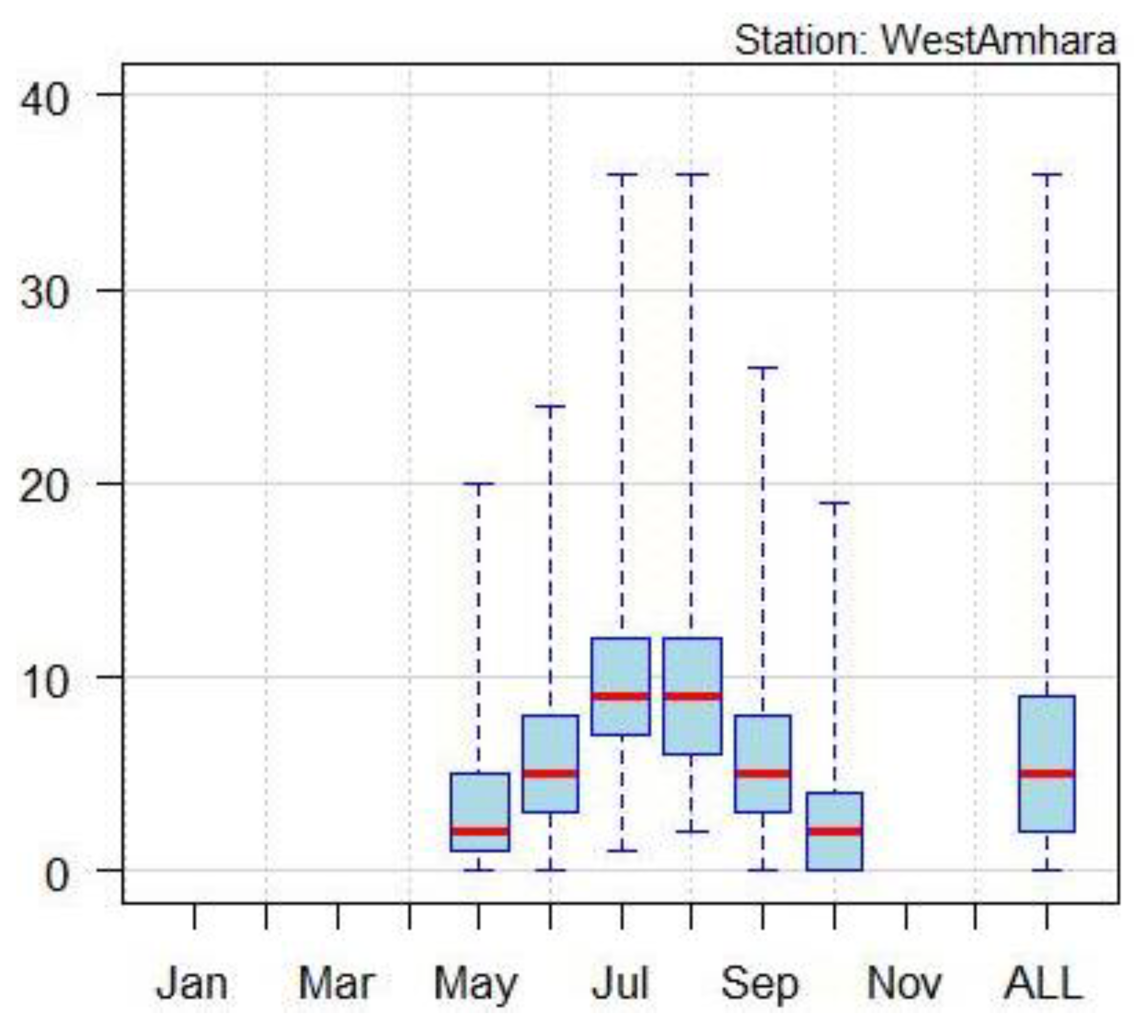
The mean daily rainfall total of Western Amhara for the period 1991-2020 is given in
Figure 2.The box and whisker plot showed that, the mean daily rainfall total was higher during July and August, and the mean daily rainfall recorded for July and August was approximately 9mm/day. During July and August ,the mean daily maximum rainfall was 35 mm/day.
Figure 2.
Box and whiskers plot representation of daily rainfall at western Amhara region for the period 1991-2020.
Figure 2.
Box and whiskers plot representation of daily rainfall at western Amhara region for the period 1991-2020.
3.1.5. Analysis of Monthly Rainfall Total
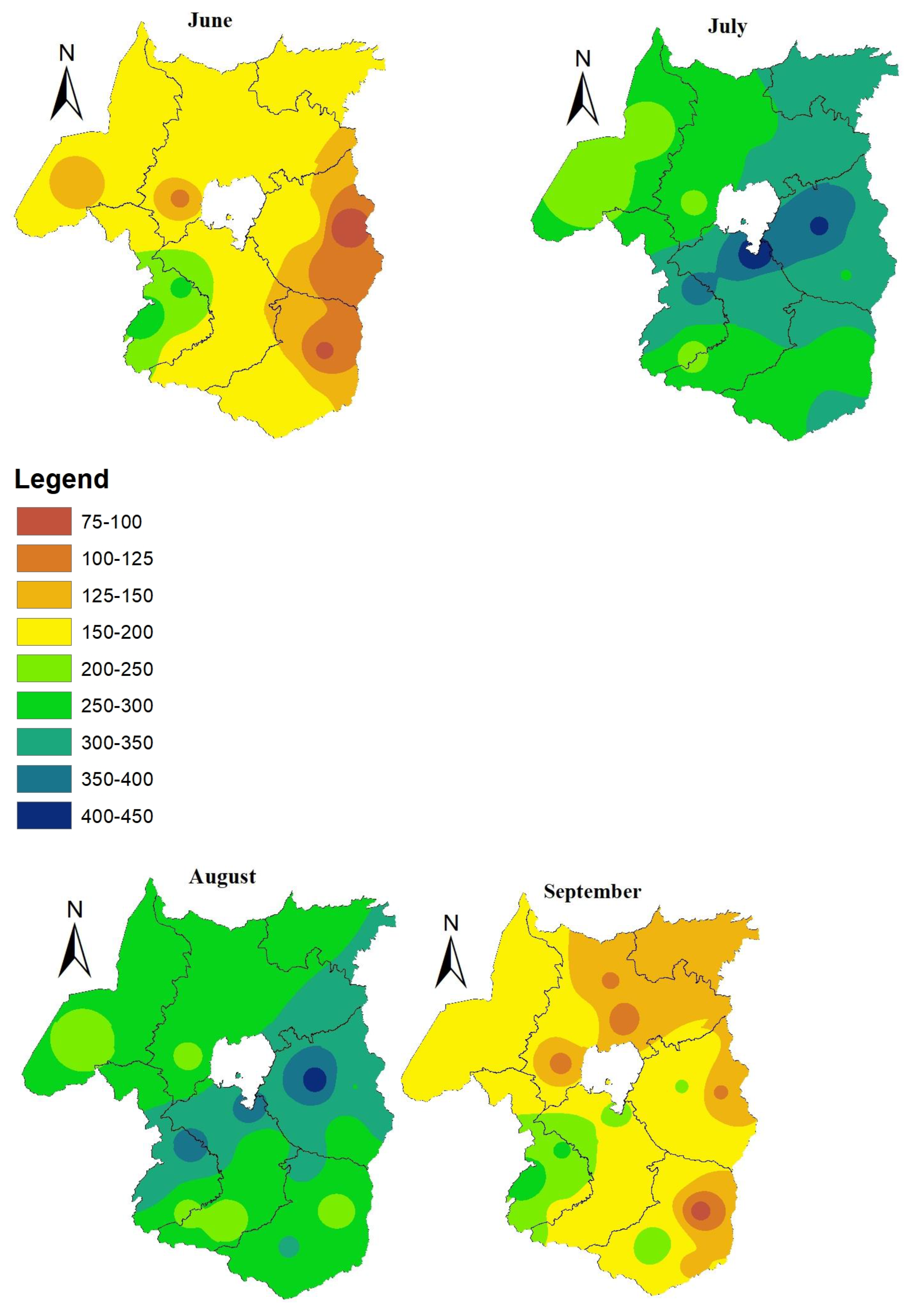
Figure 3 shows the spatial analysis of monthly rainfall for 1991-2020.During June, most areas of Western Amhara received from 125 to 200 mm rainfall, but western part acquires from 200 to 300 mm rainfall. During, July and August the rainfall distribution increased in amount and reached peak. Hence, the amount of rainfall recorded reached up to 450mm/month in July and August. The findings of Taye
et al.(2013) reveal that, the Amhara National Regional State receives much of the rainfall in June, July, August and September. The mean monthly rainfall of June, July, August, and September for the period 1991-2020 over Western Amhara region was 163.6mm,302.3mm,291.4mm,and 169.5mm respectively. Among the 20 sample stations in the Western Amhara ,Debre Tabor, Bahir Dar, and Dangila acquires better rainfall amount than others. Starting from September, the rainfall amount becomes decrease from eastern part of the region and shifts towards western part gradually, as the rain bring meteorological systems during the season becomes weaken. Overall, Western tip of the region acquires better rainfall amount than northern and eastern part of the region.
Figure 3.
Monthly rainfall (mm) analysis of west Amhara region for the period 1991-2020.
Figure 3.
Monthly rainfall (mm) analysis of west Amhara region for the period 1991-2020.
3.1.6. Analysis of Seasonal Rainfall Total
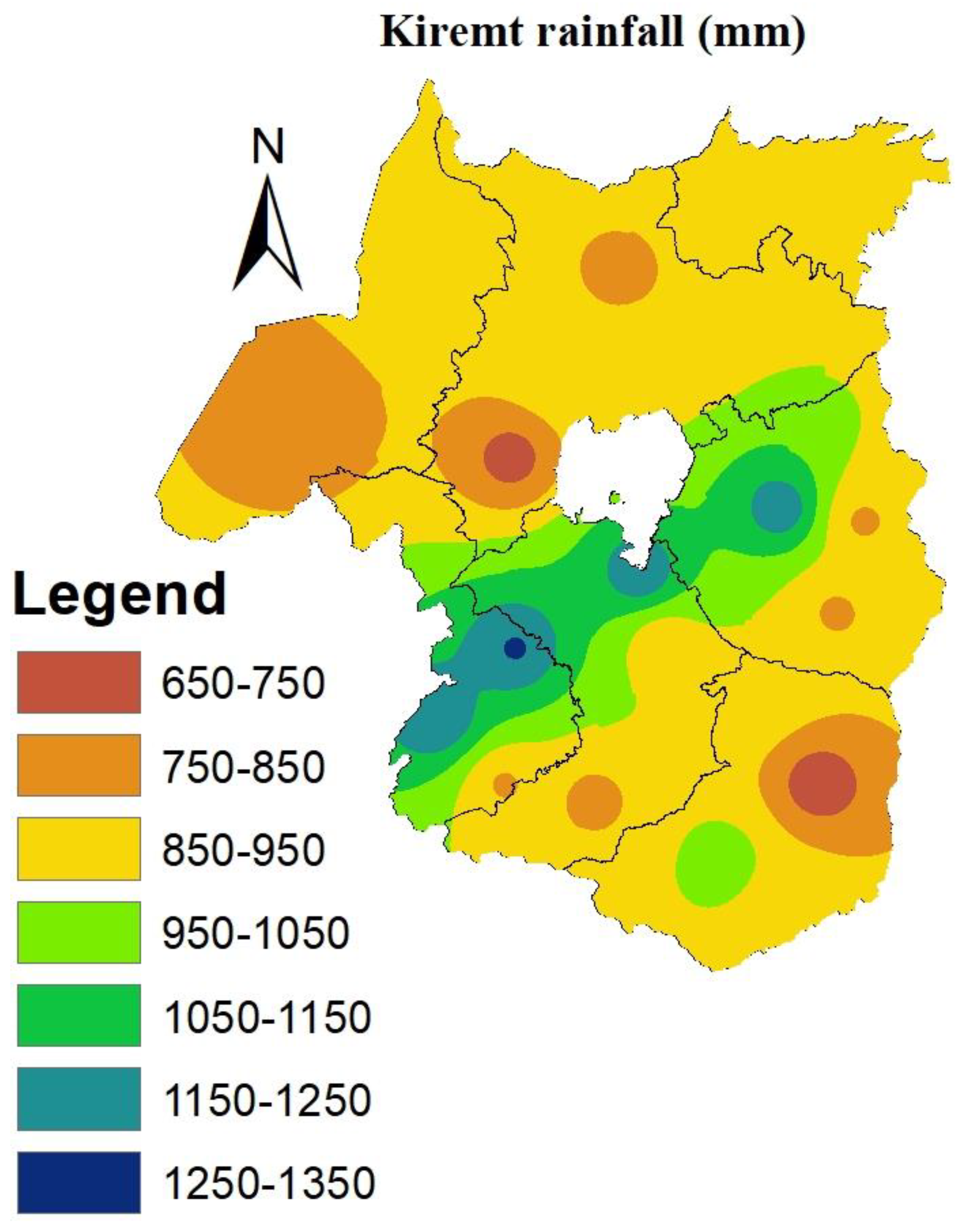
Figure 4 and
Table 8 showed the kiremt season rainfall distribution of the Western Amhara. The spatial distribution indicated that, there was variation in rainfall distribution and amount. Among the 20 sample stations, low amount of rainfall was recorded at Debre Work and Shahura with seasonal rainfall total of 650 to 750 mm/
kiremt season. However, high
total kiremt rainfall was recorded in Dangila from 1250 to 1350 mm .Most of the region recorded 850 -950 mm during the
kiremt season. The mean
kiremt rainfall in Western Amhara for the period 1991-2020 was 926.8mm. Overall, the western and central parts of the region acquired better mean
kiremt rainfall for the period 1991-2020.A study by Taye
et al.(2013) over small scale areas of Western Amhara from 1979 to 2008 showed that, the mean annual rainfall during the
kiremt season in western Amhara was 1054.2 mm.
The PCI values for
kiremt rainfall are listed in
Table (8).The results indicated that, the PCI value of
kiremt rainfall ranged from 8.4 to 10.8,with regional mean PCI value of 9.2%. Overall, the PCI value was less than 10 for regional and for most stations during the study time period, which indicated that there was uniform monthly rainfall distribution of kiremt rainfall. But at Nefas Mewucha and Debre Work stations ,there was moderate concentration of monthly rainfall for the
kiremt season. A study by Taye
et al.(2013) indicated that, Precipitation Concentration Index (PCI) value indicates that western Amhara is characterized by high to very high monthly rainfall concentration.
Table 8.
Station wise and regional mean monthly and seasonal rainfall (mm) and PCI (%) for the period 1991-2020.
Table 8.
Station wise and regional mean monthly and seasonal rainfall (mm) and PCI (%) for the period 1991-2020.
| Station |
June |
July |
August |
September |
Kiremt |
PCI (%) |
| Chagini |
286.4 |
333.4 |
342.8 |
284.4 |
1247.0 |
8.4 |
| Adet |
153.3 |
299.9 |
256.4 |
158.2 |
867.8 |
9.0 |
| Ayehu |
185.6 |
224.5 |
235.4 |
193.6 |
839.0 |
8.4 |
| Aykel |
199.2 |
291.8 |
274.7 |
170.4 |
936.1 |
8.7 |
| BahirDar |
195.2 |
450.5 |
379.5 |
212.3 |
1237.6 |
9.4 |
| Dangla |
259.5 |
368.7 |
376.9 |
255.8 |
1260.9 |
8.6 |
| Debark |
157.2 |
329.8 |
296.2 |
125.7 |
909.0 |
9.6 |
| Debre Markos |
178.9 |
281.9 |
304.9 |
229.1 |
994.9 |
8.6 |
| Debre Tabor |
175.1 |
411.6 |
426.7 |
204.9 |
1218.3 |
9.5 |
| Gondar |
174.7 |
302.4 |
297.0 |
110.4 |
884.6 |
9.5 |
| Layber |
171.7 |
254.5 |
221.2 |
169.9 |
817.3 |
8.6 |
| Metema |
182.9 |
226.9 |
264.5 |
193.2 |
867.5 |
8.5 |
| Motta |
127.4 |
324.1 |
313 |
169.3 |
933.9 |
9.5 |
| Nefas Mewucha |
74.0 |
343.8 |
299.6 |
120.7 |
838.2 |
10.8 |
| Shahura |
116.4 |
235.0 |
234.9 |
114.6 |
700.8 |
9.3 |
| simada |
101.2 |
297.6 |
287.7 |
150.9 |
837.4 |
9.7 |
| Yetnora |
153.4 |
309.3 |
288.8 |
143.2 |
894.6 |
9.3 |
| Quara |
135.6 |
214.2 |
231.4 |
172.2 |
753.4 |
8.7 |
| DebreWork |
93.7 |
271.3 |
223.6 |
87.8 |
676.4 |
10.2 |
| Sanja |
151.1 |
274.6 |
272.5 |
122.6 |
820.8 |
9.3 |
| West Amhara |
163.6 |
302.3 |
291.4 |
169.5 |
926.8 |
9.2 |
3.2. Performance Evaluation of CMIP6 GCMs for Future Rainfall Analysis
The performances of the five CMIP6 GCMs in simulating the main rainy season future rainfall characteristics of the Western Amhara region are shown in
Table (9). Acording to CRI, EC-Earth3 is the best performing CMIP6 GCMs model over Western Amhara at daily time scale. Followed by EC-Earth3, Ec-Earth3- Veg, MPI-ESM1-2-LR, and GFDL-ESM4 are the second and third best performing models for simulating rainfall characteristics of the region. But at monthly timescale,GFDL-ESM4,EC-Earth3,and Ec-Earth3-Veg are the first, second, and third best performing CMIP6 GCMs to detect rainfall total respectively. MPI-ESM1-2-LR is the poorest performing model to detect rainfall total over Western Amhara region at monthly time scale. At seasonal (
kiremt) timescale, BCC-CSM2-MR, GFDL-ESM4,and EC-Earth3 are first, second, and third best performing CMIP6 GCMs to detect
kiremt rainfall total respectively. Moreover, MPI-ESM1-2-LR underestimate (positive PBIAS) the daily, monthly, and
kiremt rainfall total over Western Amhara by 25.20%,but EC-Earth3 and Ec-Earth3-Veg overestimate (negative PBIAS) over the region at all temporal scales. In addition, GFDL-ESM4 and BCC-CSM2-MR underestimate daily to
kiremt rainfall toal by 6.70% and 11.10% respectively (
Table 9).
In general, models have different performance in different temporal scale. The top ranked four models those demonstrate relatively best performance for simulating future rainfall characteristics over Western Amhara region at daily time scale are EC-Earth3, Ec-Earth3-Veg,-MPI-ESM1-2-LR,and GFDL-ESM4.Similar to my findings, the MPI-ESM1-2-LR, EC-Earth3, and Ec-Earth3-Veg are the best performing models in simulating daily rainfall in the Bale Eco Region ,in Southern Ethiopia by Gashaw et al.(2024). Moreover, this study used the ensemble mean of the best performoing four models EC-Earth3, Ec-Earth3-Veg, MPI-ESM1-2-LR,and GFDL-ESM4 for simulating future rainfall characteristics over the Westren Amhara region on a daily time scale, while the ensemble mean of GFDL-ESM4, EC-Earth3,and Ec-Earth3-Veg were used for future monthly rainfall analysis and BCC-CSM2-MR, GFDL-ESM4,and EC-Earth3 for future Kiremt rainfall analysis over the Western Amhara region. Gashaw et al. (2024) also used asimilar approach to study future rainfall characteristics over the Bale Eco Region ,in Southern Ethiopia, and Kamruzzaman et al.(2023) also used the ensemble mean of bias-corrected CMIP6 GCMs for future rainfall and temperature projections of Bangladish for the period 2015 to 2100 under different SSPs.
3.3. Analysis of the Future Rainfall Characterstics
3.3.1. Analysis of Onset Date
The earliest, latest, mean, standard deviation, and CV of the onset date are given in
Table (10) and Appendix Figure 4-6.The earliest onset date is 124 DOY for the time period 2021-2050.The earliest onset dates ranged from 124 DOY to 174 DOY for the period 2021-2100 under SSP2-4.5, SSP3-7.0,and SSP5-8.5 ,and a high shift of onset date will be expected under SSP3-7.0 for the time period 2051-2080.The mean onset dates under SSP2-4.5 will be 148 DOY,151 DOY, and 153 DOY for 2021-2050, 2051-2080, and 2081-2100 respectively. In the case of SSP3-7.0, the mean onset dates are projected to be 160 DOY,181 DOY, and 172 DOY for the period 2021-2050,2051-2080,and 2081-2100 respectively. In addition, the mean onset date under SSP5-8.5 are projected as,144 DOY,141 DOY, and 153 DOY for the period 2021-2050,2051-2080,and 2081-2100 respectively (
Table 10).In opposite with my finding, Tegegn, (2015) conclude the expectation of early onset of
kiremt rainfall for the future over North Eastern Amhara. The CV of onset date will be less than 20,which means less variable from one season of the year to the other under all considered SSPs and time period. According to SSP3-7.0 scenario, late start of rainy season will be observed as of 202 DOY for the period 2081-2100.A study by Kwawuvi
et al.(2022) revealed that, there will be an increase in the onset date for the period 2021-2050 from 8-May (128 days) to 24 May (144 days) under the RCP4.5 and RCP8.5 emission scenarios in the Oti River Basin, West Africa.
A summary of the Mankendall trend test statistics for the mean onset date of Western Amhara region for the time period 2021-2100 under SSP2-4.5,SSP3-7.0,and SSP5-8.5 scenarios is given in
Table (11).The results revealed that, there will be a delay in the onset date (trend increase) under SSP2-4.5 for the period 2051-2080 and 2081-2100,under SSP3-7.0 for the period 2021-2050,under SSP5-8.5 for the period 2081-2100.But the delay onset date will be significant at 95% confidence level under SSP3-7.0 for the period 2021-2050 (P<0.05) by 1.08 day/year. On the other hand, for most of projected time period and for SSP2-4.5,SSP3-7.0,and SSP5-8.5 there will be earliest onset date (decreasing trend) ,but insignificant at 95% confidence level (
Table 11).A study by Wasihun
et al.(2020) ,showed an increasing and significant onset date at 95% confidence level for the period 2018-2047 over Gelemso, West Harerghe in Ethiopia.
3.3.2. Analysis of Cessation Date
Table 12 and Appendix Figure 7-9 showed the result of early, late, mean, standard deviation, and CV of the cessation date for Western Amhara region for the period 2021-2100 under SSP2-4.5, SSP3-7.0, and SSP5-8.5.The result revealed that, the early cessation date ranged from 248 DOY to 261 DOY under SSP2-4.5,233 DOY to 238 DOY under SSP3-7.0,and 246 DOY to 261 DOY under SSP5-8.5 for the period 2021-2100.The cessation date will be extended to 288-303 DOY under SSP-4.5, 266-282 DOY under SSP3-7.0,and 283-288 DOY under SSP5-8.5 for the period 2021-2100. Projected mean cessation date of the Wesern Amhara region will be earlier than the baseline mean cessation date by 29 days for the period 2021-2050, 27 days for the period 2051-2080,and 32 days for the period 2081-2100 under SSP2-4.5.In the case of SSP3-7.0,the cessation date projected to be earlier by 36 days ,52 days, and 52 days for the period 2021-2050,2051-2080,and 2081-2100 respectively. On the otherhand ,the cessation date will be earlier by 28 days, 18 days, and 33 days under SSP5-8.5 for the period 2021-2050, 2051-2080, and 2081-2100 respectively. A study by Kwawuvi
et al.(2022) in the Oti River basin, West Africa, indicated that, Cessation date which was on 29 October (302 DOY) in the historical period (1981-2010) could decrease to 7 October (280 DOY) under both RCP4.5 and RCP8.5 scenarios in 2021-2050. The CV of the mean cessation date for the period 2021-2100 and for all scenarios considered in this study is projected to be less than 10,which implied that less variable from one season of the year to the other.
Table 13 showed modified mankendal trend test analysis of mean cessation date of Western Amhara region for the period 2021-2050,2051-2080,and 2081-2100 under SSP2-4.5,SSP3-7.0,and SSP5-8.5 scenarios. From the analysis, the mean cessation date of Western Amhara region for the period 2021-2050 under SSP2-4.5,for the period 2051-2080 and 2081-2100 under SSP 3-7.0,and for the period 2021-2050 under SSP5-8.5 scenario showed increasing trend (becomes late),but it is not significant at 95% confidence level. On the other hand, the mean cessation date of Western Amhara region, showed decreasing trend (cessation becomes earlier),during the period 2051-2080 and 2081-2100 (under SSP2-4.5),during 2021-2050 (under SSP3-7.0),and during 2051-2080 and 2081-2100 (under SSP5-8.5).However, the trend is significant and decreasing only for the period 2021-2050 under the SSP3-7.0 scenario with Sen’s slope estimator of 0.54 day/year.
3.3.3. Analysis of Length of Growing Season
Table 14 and Appendix Figure 10-12 showed the mean length of growing period for the study time interval 2021-2100 under SSP2-4.5,SSP3-7.0,and SSP5-8.5 scenario for Western Amhara region. The result revealed that, the minimum length of growing period for the period 2021-2050, 2051-2080, and 2081-2100 projected to be 93, 93, and 72 under SSP2-4.5 respectively, for the period 2021-2050 (60),2051-2080 (35),2081-2100 (35) under SSP3-7.0,and for the period 2021-2050 (99),2051-2080 (89),and 2081-2100 (72) under the SSP5-8.5 scenario, while the maximum length of the growing period is projected to be during 2021-2050 (147), 2051-2080 (143), 2081-2100 (145) under SSP2-4.5.For SSP3-7.0,the maximum length of the growing period extends to 146 (2021-2050), 95 (2051-2080), and 108 (2081-2100).Moreover, in the case of the SSP5-8.5,the maximum length of growing period is projected to be 125 (2021-2050),148 (2051-2080),145 (2081-2100).The mean season length of the Western Amhara region for the baseline (1991-2020) was 142 days (
Table 6).For projected time period under different scenarios, the length of the growing period will be shortened by 23 days (2021-2050), 25 days (2051-2080),31 days (2081-2100) under SSP2-4.5.In addition the main rainy season length is expected to be shortened by 41 days (2021-2050) ,78 days (2051-2080), and 69 days (2081-2100) under the SSP3-7.0 scenario, and the mean length of the growing season for the Western Amhara region is projected to be 17 days (2021-2050),12 days (2051-2080),and 31 days (2081-2100) under the SSP5-8.5. Model projections have also shown moderate reduction (< 20%) in the length of the growing period across Africa including Ethiopia (Thornton
et al. 2009).Another study by Kwawuvi
et al.(2022) in the Oti River Basin, West Africa, indicated that, season length would decrease from 173 days to approximately 136 days under both RCP4.5 and RCP8.5 scenarios in 2021-2050. The average deviation of the length of the growing period from the mean length of the growing period ranged from 13 days during 2051-2080 under SSP5-8.5 to 29 days during 2021-2050 under SSP3-7.0.The season length of Western Amhara region was moderately variable (CV<30%) under SSP3-7.0 during study time period 2021-2050,2051-2080,and 2081-2100. However, the season length was projected to be less variable for SSP2-4.5 and SSP5-8.5 for all considered study time periods.
Table 15 shows the Mankendall trend test analysis of mean season length of Western Amhara region for the period 2021-2100 under SSP2-4.5,SSP3-7.0, and SSP5-8.5 scenarios. Th result showing that there will be increasing trend of season length for the period 2021-2050 and 2081-2100 under SSP2-4.5 scenario, during 2051-2080 and 2081-2100 under SSP3-7.0 Scenario, and during 2021-2050 and 2051-2080 under SSP5-8.5 scenario, But the increasing trend of mean season length is not significant at 95 % confidence level (p>0.05).On the other hand, the mean season length of the Western Amhara region projected to decrease during 2051-2080 under-SSP2-4.5,from 2021 to 2050 under SSP3-7.0,and from 2081 to 2100 under SSP5-8.5 scenario; however the decreasing trend (shorten season length) would be significant during 2021-2050 under SSP3-7.0 with Sen’s slope estimator of 2.17 days/year. A study by Hadgu
et al.(2015) also reported a decrease in LGP in northern Ethiopia.
3.3.4. Analysis of Daily Rainfall Total
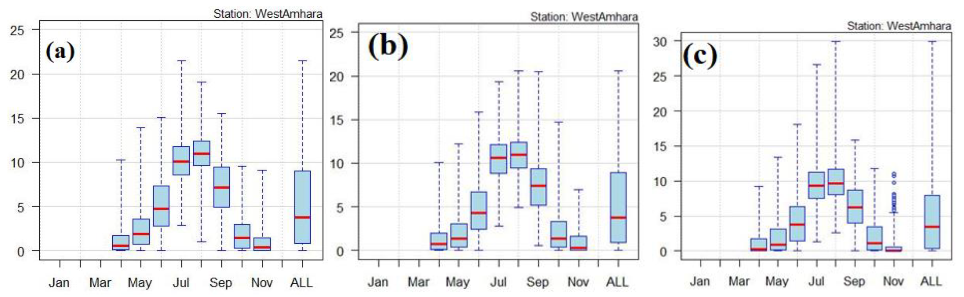
Figure 5 shows the box and whisker plot representation of mean daily rainfall under SSP2-4.5 during the time period 2021-2100.The results show that, the daily mean rainfall projected to be 4mm /day (June),10mm/day (July),11mm/day (August),and 7mm/day (September) for the period 2021-2100. Moreover, for the period 2051-2080,the daily mean rainfall projected to be 4mm/day (June),10.5mm/day (July),11mm/day (August),and 7mm/day (September) under SSP2-4.5.However,from 2081-2100 under SSP2-4.5 the mean daily rainfall projected for July and August will be less than 10mm/day. Lee
et al.(2011), showed that in the 21
st century the annual number of rainy days in Hong Kong is expected to decrease while the daily rainfall intensity will increase.
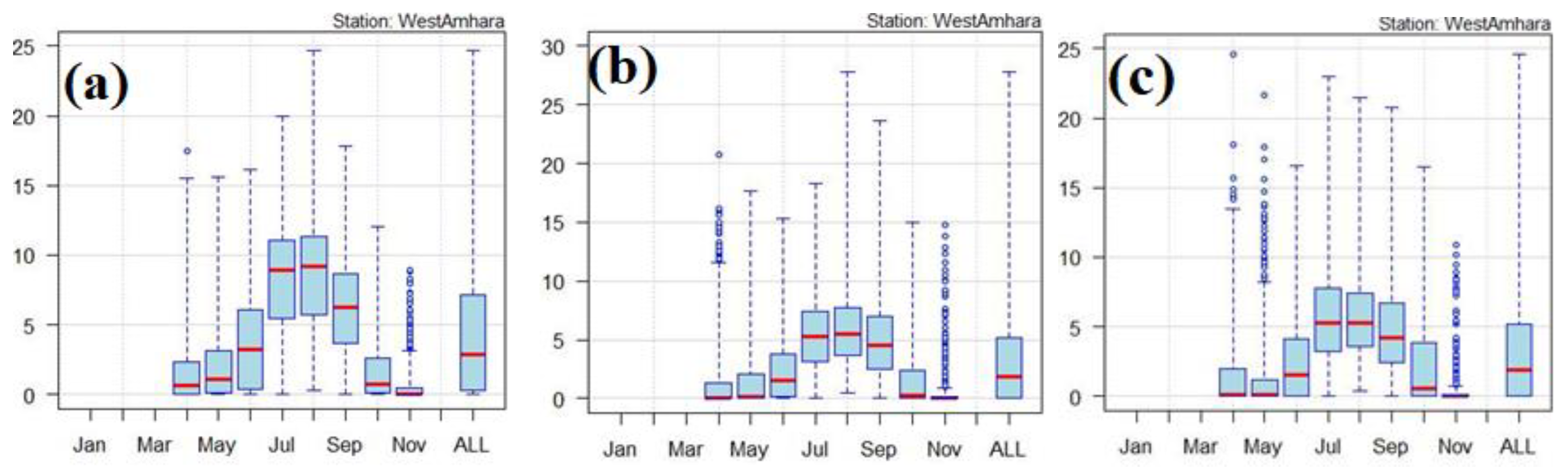
Figure 6 dipicts the box and whisker plot representation of mean daily rainfall for the period 2021-2100 under SSP3-7.0 for the Western Amhara region, showing that, the projected mean daily rainfall for the period 2021-2100 will be diminished under 10mm/day including the July and August months of the season. However, under such a scenario, there is a probability of the occurrence of un-seasonal rainfall before and after the start of the main rainy season.
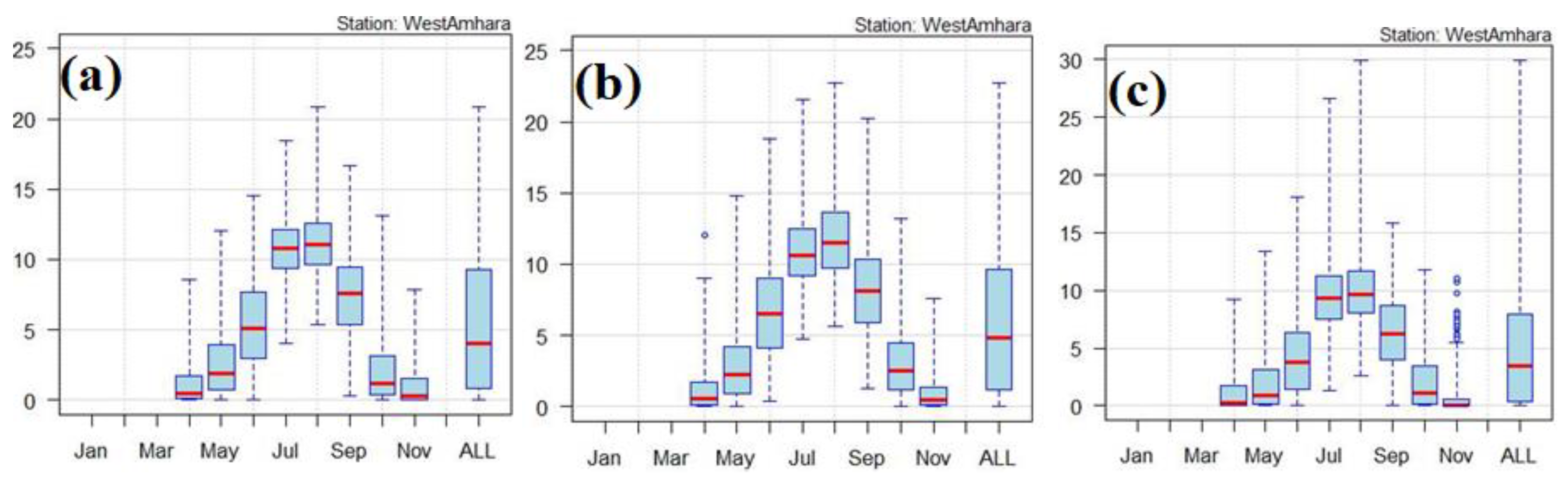
Figure 7 shows the box and whisker plot representation of the mean daily rainfall for the period 2021-2100 under SSP5-8.5.The results show that, the projected mean daily rainfall will be higher than 10mm/day during July and August months for time period 2021-2050 and 2051-2080.However the mean daily rainfall in July and August is projected to diminish under 10mm/day for the period 2081-2100 under the SSP5-8.5 scenario. Overall, the mean daily rainfall will be higher during the months of July and August and reach extreme values during August than July over the Western Amhara region for the projected time period and for all considered scenarios.
3.3.5. Analysis of Monthly and Seasonal Rainfall Total
Table 16 shows the projected mean monthly and seasonal rainfall of the Western Amhara region for the period 2021-2100 under SSP2-4.5,SSP3-7.0,and SSP5-8.5 scenarios, showing that, the mean monthly and seasonal rainfall for the period 2051-2080 is projected to be better than the period 2021-2050 and 2081-2100 under the SSP2-4.5 scenario. According to SSP3-7.0 ,the mean monthly and seasonal rainfall of Western Amhara region is expected to be good during 2021-2050 as compared with 2051-2080 and 2081-2100.On the other hand the mean monthly and seasonal rainfall of the main rainy season projected to be better for the period 2051-2080 under SSPP5-8.5 scenario. A study by Tegegn, (2015) for the period 1992-2012 ,also showed the average agreed of GCM models in increasing
kiremt seasonal rainfall total by 2030s under RCP 4.5 (Representative Concentration Pathways 4.5) emission scenario. Overall, Western Amhara region projected to acquire better rainfall amount during July and August than June and September months under all considered scenarios and projected time periods. More over, the highest projected seasonal rainfall will be 1036.5mm/year for the period 2051-2080 under SSP2-4.5 scenario. For the period 2081-2100,the seasonal
kiremt rainfall expected to decrease as compared with baseline seasonal rainfall under SSP2-4.5, SSP3-7.0, and SSP5-8.5 scenario. In line with my study , a study conducted by Arndt
et al.(2011) showed decreasing of
Kiremt rainfall by 5-6% by 2080s in Ethiopia. A study by Wasihun
et al.(2020) also showed ,the decrease projected
kiremt season rainfall amount in West Harerghe, Oromia Ethiopia. Another study by Alaminie
et al.(2021) ,found that, there will be slight increasing trend of rainfall over Abay basin under low (SSP1-2.6) to strong (SSP5-8.5) forcing scenarios for the period 2031 to 2100. Ayalew
et al.(2012) showed that, the amount of annual rainfall and number of rainy days also decreased in north western Ethiopia in the 2080s. A study by Wasihun
et al.(2020) showed that, the
kiremt rainfall amount will be decreased by about 0.16 mm per year during the study period 2018 to 2047.A study by Bekele, (n.d.) also showed the expectation of a slight decrease in
kiremt rainfall for the Robe and Sinana stations for the period 2020-2049.
4.Conclusions
This study concerns the characterization of past and future rainfall characteristics of the main rainy season (Kiremt) over Western Amhara region. The onset date, cessation date, and length of growing period of observed rainfall varies from place to place. Western part of the study area acquire early start of rainy season ,late cessation of the rainy season ,and have long season length than the eastern part of the region. The start of the rainy season for observed rainfall (1991-2020) showed non significant decreasing trend (early onset) for most selected stations. The cessation date of Western Amhara showed increasing and significant trend at 95% confidence level with Sen’s slope estimator of 0.35 day/year. But for most areas of Western Amhara region, the mean onset date and cessation date of the rainy season was May and October months respectively. Hence, the mean onset date and cessation date of Western Amhara region for the period 1991-2020 was 138 DOY (17-May) and 297 DOY (23-October) respectively. Due to this, the mean season length of the region was 142 days. The region acquires better rainfall amounts during July and August months, and the western and central parts of the study area recorded better daily, monthly, and seasonal rainfall amounts than the rest of the region. Most areas of Western Amhara recorded 850 to 950 mm during the period 1991-2020.In addition, the years 2020,2022,and 2019 were wettest years, the years 1995,1997,and 2015 were driest years.
The future rainfall characteristics of Western Amhara for the main rainy season were determined under the sixth phase Coupled Model Intercomparision Project phase 6 (CMIP6) Socio Economic Pathways (SSPs) scenario projection. Performance evaluation result of CMIP6 GCMs showed that, the ensemble mean of EC-Earth3,Ec-Earth3-Veg,MPI-ESM-2 -LR ,and GFDL-ESM4, GFDL-ESM4, EC-Earth3,and Ec-Earth3-Veg,BCC-CSM-2-MR, GFDLESM4,and EC-Earth3 were used for future daily, monthly and seasonal rainfall studies respectively, under different Shared Socioeconomic Pathways (SSPs),which means SSP2-4.5,SSP3-7.0,and SSP5-8.5 scenarios for the period 2021-2100 after appropriate bias correction.
The mean onset date of the Western Amhara region will be late from baseline mean onset date by 10 days,13 days, and 15 days for the period 2021-2050,2051-2080,and 2081-2100 respectively under SSP2-4.5.In addition, the projected mean onset date will be delayed from 22 to 48 days under SSP3-7.0 scenario and from 3 to 15 days under SSP5-8.5 scenario. According to SSP3-7.0 scenario, the future start of the rainy season will be late. Regarding to this scenario, radical shift of start during rainy season will be recorded from May (mostly baseline onset) to June. In the considered projected time period and scenario, the trend of onset date showed both early and late start in different areas of the region. But statistically significant and delayed onset date at 95 % confidence level will be recorded for the period 2021-2050 with Sen’s slope estimator of 1.08 day/year. The mean cessation date will be earlier than the baseline mean (1991-2020) by 29,27 ,and 32 days for the period 2021-2050,2051 2080,and 2081-2100 respectively uder SSP2 4.5.Moreover,the mean cessation date will be earlier by 36 days,52 days and 52 days for the period 2021-2050,2051-2080,and 2081-2100 under SSP3-7.0 respectively. In the case of SSP5-8.5,the mean cessation date of the rainy season will be earlier by 28 days,18 days, and 33 days for the period 2021-2050,2051-2080, and 2081-2100 respectively. In few considered time period, cessation date will late, but significant and decreasing cessation date at 95% confidence level will be observed for the period 2021-2050 under SSP3-7.0 with Sen’s slope estimator of 0.54 day/year. As aresult of late onset and early cessation date expectation over Western Amhara region, the season length expeted to be shorten by 23 to 31 days under SSP2-4.5 Scenario,41 to 78 days under SSP3-7.0 scennario, and 12 to 31 days under SSP5-8.5 scenario. But significant and short season length will be record for the period 2021-2050 under SSP3-7.0 with Sen’s slope estimator of 2.17 days/year. The months of July and Agust will have high contribution for kiremt rainfall total like their contribution for the past. For projected time period except for SSP5-8.5 during 2051-2080,the mean rainfall total of June decrease as compared with baseline. But the overall mean seasonal rainfall total of the main rainy season will increase as compared with baseline under SSP2-4.5 and SSP5-8.5,but not according to SSP3-7.0 scnario. According to SSP3-7.0,main rainy seasons from 2036 to 2050 will be drier season.
Due to the expectation of late onset date, early cessation date ,and short season length of the main rainy season over the study area, design possible adaptation and mitigation strategies effectively among farmers, researchers, decision makers ,and others is crucial. In addition attention should be paid to new and emerging water conservation and supplement irrigation system should be implemented to overcome failure of agricultural production during eratic and dry spell condition sine the livelihood of the study region mainly agriculture based. Eventhouth, the future season of the main rainy season expected to be shorten, the amount of rainfall obtained with in the season will increase according to some scenarios. Hence, ground and underground water harvesting should be practiced (accomplished effectively).In addition improved seed selection for short season length should be practiced effectively, and the results of any model should depend on the quality of the input data; therefore to increase the reliability of future rainfall studies to be more reliable, complete, suitable for design adaptation strategies, and specific for the decision-making process, it is recommended to conduct similar studies with a large number of meteorological stations and CMIP6 GCMs models for the agroecological zones of Western Amhara.
Author Contributions
Tewabech Tesema: Conceptualization, Data Organization; Methodology, Data analysis and interpretation, original draft and writing, review ,and editing; Gashaw Bimirew: Data organization, Methodology, review & editing; Endeg Aniley: Data organization and Methodology; Tilahun Wubu: Data organization, review & editing.
Funding
This study received no funding.
Data Availability Statement
Climatic data are available from the corresponding author upon request.
Acknowledgments
The authors acknowledge the Ethiopian Meteorology Institute (EMI) for providing observed rainfall data. We are also grateful to the producers of CMIP6 GCMs models for providing data available without charge. The authors are also grateful to the Western Amhara Meteorology Service Center staf for their contributions.
Conflicts of Interest
The authors declare no conflict of interest.
References
- Ageet, S., Fink, A. H., Maranan, M., Diem, J. E., Hartter, J., Ssali, A. L., & Ayabagabo, P. (2022). Validation of Satellite Rainfall Estimates over Equatorial East Africa. JOURNAL OF HYDROMETEOROLOGY, 23.
- Alaminie, A. A., Tilahun, S. A., Legesse, S. A., Zimale, F. A., Tarkegn, G. B., & Jury, M. R. (2021). Evaluation of Past and Future Climate Trends under CMIP6 Scenarios for the UBNB (Abay), Ethiopia. Water, 13(15), 2110. [CrossRef]
- Amekudzi, L. K., Yamba, E. I., Preko, K., Asare, E. O., Aryee, J., Baidu, M., & Codjoe, S. N. (2015). Variabilities in rainfall onset, cessation and length of rainy season for the various agro-ecological zones of Ghana. Climate, 3(2), 416–434.
- Aniley, E., Gashaw, T., Abraham, T., Demessie, S. F., Bayabil, H. K., Worqlul, A. W., van Oel, P. R., Dile, Y. T., Chukalla, A. D., Haileslassie, A., & Wubaye, G. B. (2023). Evaluating the performances of gridded satellite/reanalysis products in representing the rainfall climatology of Ethiopia. Geocarto International, 38(1), 2278329. [CrossRef]
- Arndt, C., Robinson, S., & Willenbockel, D. (2011). Ethiopia’s growth prospects in a changing climate: A stochastic general equilibrium approach. Global Environmental Change, 21(2), 701–710.
- Arrieta-Castro, M., Donado-Rodríguez, A., Acuña, G. J., Canales, F. A., Teegavarapu, R. S. V., & Kaźmierczak, B. (2020). Analysis of Streamflow Variability and Trends in the Meta River, Colombia. Water, 12(5), 1451. [CrossRef]
- Asfaw, A., Simane, B., Hassen, A., & Bantider, A. (2018). Variability and time series trend analysis of rainfall and temperature in northcentral Ethiopia: A case study in Woleka sub-basin. Weather and Climate Extremes, 19, 29–41.
- Ayalew, D., Tesfaye, K., Mamo, G., Yitaferu, B., & Bayu, W. (2012). Outlook of future climate in northwestern Ethiopia. Agricultural Sciences, 03(04), 608–624. [CrossRef]
- Ayehu, G. T., Tadesse, T., Gessesse, B., & Dinku, T. (2018). Validation of new satellite rainfall products over the Upper Blue Nile Basin, Ethiopia. Atmospheric Measurement Techniques, 11(4), 1921–1936. [CrossRef]
- Bazezew, A. (2012). Determining Food Security Indicators at Household Level in Drought Prone Areas of the Amhara Region of Ethiopia: The Case of Lay Gaint District, Amhara Regional State. Ethiopian Journal of Environmental Studies and Management, 5(4), 422–434.
- Bekele, F. (n.d.). CHARACTERIZING CURRENT AND FUTURE RAINFALL VARIABILITY AND ITS EFFECT ON WHEAT AND BARLEY PRODUCTION IN SINANA DISTRICT, SOUTH EASTERN ETHIOPIA.
- Belay, A. S., Fenta, A. A., Yenehun, A., Nigate, F., Tilahun, S. A., Moges, M. M., Dessie, M., Adgo, E., Nyssen, J., Chen, M., Griensven, A. V., & Walraevens, K. (2019). Evaluation and Application of Multi-Source Satellite Rainfall Product CHIRPS to Assess Spatio-Temporal Rainfall Variability on Data-Sparse Western Margins of Ethiopian Highlands. Remote Sensing, 11(22), 2688. [CrossRef]
- Belazreg, N. E. H., Hasbaia, M., Şen, Z., & Ferhati, A. (2023). Historical evaluation and future projections of monthly precipitation and temperature under CMIP6 GCMs, case of Hodna basin (central Algeria). Arabian Journal of Geosciences, 16(1), 39.
- Berhanu, D., Alamirew, T., Taye, M. T., Tibebe, D., Gebrehiwot, S., & Zeleke, G. (2023). Evaluation of CMIP6 models in reproducing observed rainfall over Ethiopia. Journal of Water and Climate Change, 14(8), 2583–2605. [CrossRef]
- Berhe, A. G., Misgna, S. H., Abraha, G. G.-S., & Abraha, A. Z. (2023). Variability and trend analysis of temperatures, rainfall, and characteristics of crop-growing season in the eastern zone of Tigray region, northern Ethiopia. Theoretical and Applied Climatology, 152(1–2), 25–43. [CrossRef]
- Camberlin, P., & Philippon, N. (2002). The East African March–May rainy season: Associated atmospheric dynamics and predictability over the 1968–97 period. Journal of Climate, 15(9), 1002–1019.
- Dangol, S., Talchabhadel, R., & Pandey, V. P. (2022). Performance evaluation and bias correction of gridded precipitation products over Arun River Basin in Nepal for hydrological applications. Theoretical and Applied Climatology, 148(3–4), 1353–1372. [CrossRef]
- De Luis, M., Gonzalez-Hidalgo, J. C., Brunetti, M., & Longares, L. A. (2011). Precipitation concentration changes in Spain 1946–2005. Natural Hazards and Earth System Sciences, 11(5), 1259–1265.
- Degefu, M. A., & Bewket, W. (2023). Drought monitoring performance of global precipitation products in three wet seasons in Ethiopia: Part I—Quasi-objective examination. Meteorological Applications, 30(4), e2143.
- Dinku, T., Faniriantsoa, R., Islam, S., Nsengiyumva, G., & Grossi, A. (2022). The climate data tool: Enhancing climate services across Africa. Frontiers in Climate, 3, 787519.
- Dinku, T., Funk, C., Peterson, P., Maidment, R., Tadesse, T., Gadain, H., & Ceccato, P. (2018). Validation of the CHIRPS satellite rainfall estimates over eastern Africa. Quarterly Journal of the Royal Meteorological Society, 144(S1), 292–312. [CrossRef]
- Evangelista, P., Young, N., & Burnett, J. (2013). How will climate change spatially affect agriculture production in Ethiopia? Case studies of important cereal crops. Climatic Change, 119(3), 855–873.
- Gashaw, T., Worqlul, A. W., Taye, M. T., Lakew, H. B., Seid, A., Ayele, G., & Haileslassie, A. (2024). Performance evaluations of CMIP6 model simulations and future projections of rainfall and temperature in the Bale Eco-Region, Southern Ethiopia. Theoretical and Applied Climatology. [CrossRef]
- Gebrechorkos, S., Taye, M. T., Birhanu, B., Solomon, D., & Demissie, T. (2023). Future changes in climate and hydroclimate extremes in East Africa. Earth’s Future, 11(2), e2022EF003011.
- Gebremichael, A., Quraishi, S., & Mamo, G. (2014). Analysis of seasonal rainfall variability for agricultural water resource management in southern region, Ethiopia. Journal of Natural Sciences Research, 4(11), 56–79.
- Gupta, H. V., Sorooshian, S., & Yapo, P. O. (1999). Status of automatic calibration for hydrologic models: Comparison with multilevel expert calibration. Journal of Hydrologic Engineering, 4(2), 135–143.
- Hadgu, G., Tesfaye, K., & Mamo, G. (2015). Analysis of climate change in Northern Ethiopia: Implications for agricultural production. Theoretical and Applied Climatology, 121, 733–747.
- Hamed, K. H., & Ramachandra Rao, A. (1998). A modified Mann-Kendall trend test for autocorrelated data. Journal of Hydrology, 204(1–4), 182–196. [CrossRef]
- Imad-eldin, A., El-Hag, F. A., Abdelkarim, A. M., & Abdalla, A. K. (2015). Changing Climate and Farming Productivity in the Drylands of Eastern Sudan. Sudan Academy of Sciences Journal Special Issue (Climate Change), 56.
- Iqbal, Z., Shahid, S., Ahmed, K., Ismail, T., Ziarh, G. F., Chung, E.-S., & Wang, X. (2021). Evaluation of CMIP6 GCM rainfall in mainland Southeast Asia. Atmospheric Research, 254, 105525.
- Kamruzzaman, M., Wahid, S., Shahid, S., Alam, E., Mainuddin, M., Islam, H. M. T., Cho, J., Rahman, M. M., Chandra Biswas, J., & Thorp, K. R. (2023). Predicted changes in future precipitation and air temperature across Bangladesh using CMIP6 GCMs. Heliyon, 9(5), e16274. [CrossRef]
- Kwawuvi, D., Mama, D., Agodzo, S. K., Hartmann, A., Larbi, I., Bessah, E., Abraham, T., Dotse, S.-Q., & Limantol, A. M. (2022). An investigation into the future changes in rainfall onset, cessation and length of rainy season in the Oti River Basin, West Africa. Modeling Earth Systems and Environment, 8(4), 5077–5095. [CrossRef]
- Lebeza, T. M., Gashaw, T., Bayabil, H. K., van Oel, P. R., Worqlul, A. W., Dile, Y. T., & Chukalla, A. D. (2024). Performance of specific CMIP6 GCMs for simulating the historical rainfall and temperature climatology of Lake Tana sub-basin, Ethiopia. Scientific African, e02387.
- Lee, T., Chan, K., Chan, H., & Kok, M. (2011). Projections of extreme rainfall in Hong Kong in the 21st century. Acta Meteorologica Sinica, 25(6), 691–709. [CrossRef]
- Lotfie, A. Y., Abdelrahman, A. K., Faisal, M. E.-H., Ahmed, M. A., Hussain, S. A., Abdelhadi, A. W., Yasunori, K., & and, I. A. A.-B. (2018). Length of the growing season for dry rainfed farming under Monsoon climate in Gedarif, Sudan. African Journal of Agricultural Research, 13(42), 2311–2323. [CrossRef]
- Lupi Edao, A., Kibert, K., & Mamo, G. (2018). Analysis of Start, End and Length of the Growing Season and Number of Rainy Days in Semi-Arid Central Refit Valley of Oromia State, Ethiopia. Advances in Crop Science and Technology, 06(04).
- Mensah, C., Amekudzi, L. K., Klutse, N. A. B., Aryee, J. N. A., & Asare, K. (2016). Comparison of Rainy Season Onset, Cessation and Duration for Ghana from RegCM4 and GMet Datasets. Atmospheric and Climate Sciences, 06(02), 300–309. [CrossRef]
- Mohammed, J. A. (2024). Performance evaluation and ranking of CMIP6 global climate models over upper blue nile (abbay) basin of Ethiopia. Natural Hazards Research, S2666592124000532. [CrossRef]
- Morales-Acuña, E., Linero-Cueto, J. R., & Canales, F. A. (2021). Assessment of Precipitation Variability and Trends Based on Satellite Estimations for a Heterogeneous Colombian Region. Hydrology, 8(3), 128. [CrossRef]
- NMSA. (1996). Climatic and agroclimatic resources of Ethiopia. Natl. Meteorol. Serv. Agency of Ethiopia, Meteorol. Res. Rep. Ser., 1(1), 1–137.
- Oguntunde, P. G., Lischeid, G., Abiodun, B. J., & Dietrich, O. (2014). Analysis of spatial and temporal patterns in onset, cessation and length of growing season in Nigeria. Agricultural and Forest Meteorology, 194, 77-87. [CrossRef]
- Oliver, J. E. (1980). MONTHLY PRECIPITATION DISTRIBUTION: A COMPARATIVE INDEX. The Professional Geographer, 32(3), 300–309. [CrossRef]
- Omay, P. O., Muthama, N. J., Oludhe, C., Kinama, J. M., Artan, G., & Atheru, Z. (2023). Evaluation of CMIP6 Historical Simulations over IGAD region of Eastern Africa. [CrossRef]
- Owusu, K., Waylen, P., & others. (2009). Trends in spatio-temporal variability in annual rainfall in Ghana (1951-2000). Weather, 64(5), 115.
- Salinger, L., & Stryker, D. (2001). Comparing and evaluating poverty reduction approaches: USAID and the evolving poverty reduction paradigm. Associates for International Resources and Development, Cambridge, MA.
- Shiru, M. S., & Chung, E.-S. (2021). Performance evaluation of CMIP6 global climate models for selecting models for climate projection over Nigeria. Theoretical and Applied Climatology, 146(1–2), 599–615. [CrossRef]
- Silva, A. T. (2017). Introduction to Nonstationary Analysis and Modeling of Hydrologic Variables. In M. Naghettini (Ed.), Fundamentals of Statistical Hydrology (pp. 537–577). Springer International Publishing. [CrossRef]
- Stern, R., Rijks, D., Dale, I., & Knock, J. (2006). INSTAT climatic guide. Statistical Services Centre, The University of Reading, UK.
- Tadese, M. T., Kumar, L., & Koech, R. (2020). Climate change projections in the Awash River basin of Ethiopia using global and regional climate models. International Journal of Climatology, 40(8), 3649–3666.
- Tadese, M. T., Kumar, L., Koech, R., & Zemadim, B. (2019). Hydro-Climatic Variability: A Characterisation and Trend Study of the Awash River Basin, Ethiopia. Hydrology, 6(2), 35. [CrossRef]
- Taye, M., Zewdu, F., & Ayalew, D. (2013). Characterizing the climate system of Western Amhara, Ethiopia: A GIS approach. American Journal of Research Communication, 1(10), 319–355.
- Tegegn, M. G. (2015). Analysis of Past and Future Intra-Seasonal Rainfall Variability and its Implications for Crop Production in the North Eastern Amhara Region, Ethiopia.
- Thornton, P. K., Jones, P. G., Alagarswamy, G., & Andresen, J. (2009). Spatial variation of crop yield response to climate change in East Africa. Global Environmental Change, 19(1), 54–65.
- Wasihun, G. F., Mengistu, M., & Lisanework, N. (n.d.). CHARACTERIZATION OF PAST AND FUTURE CLIMATE VARIABILITY OF HABRO DISTRICT, WEST HARERGHE ZONE, OROMIA, ETHIOPIA. 7.
- Worku, G., Teferi, E., Bantider, A., & Dile, Y. T. (2020). Statistical bias correction of regional climate model simulations for climate change projection in the Jemma sub-basin, upper Blue Nile Basin of Ethiopia. Theoretical and Applied Climatology, 139, 1569–1588.
- Zeleke, A., Tesfaye, K., Tadesse, T., Alem, T., Ademe, D., & Adgo, E. (2023). Spatiotemporal analysis of rainfall and temperature variability and trends for climate resilient maize farming system in major agroecology zones of northwest Ethiopia. International Journal of Agricultural Sustainability, 21(1), 2255450. [CrossRef]
Figure 1.
Location Map of Western Amhara from Ethiopia.
Figure 1.
Location Map of Western Amhara from Ethiopia.
Figure 4.
Seasonal rainfall (mm) analysis of west Amhara region for the period 1991-2020.
Figure 4.
Seasonal rainfall (mm) analysis of west Amhara region for the period 1991-2020.
Figure 5.
Box and whiskers plot representation of daily rainfall for western Amhara region under SSP2-4.5 for the period 2021-2050 (a),2051-2080 (b),and 2081-2100(c).
Figure 5.
Box and whiskers plot representation of daily rainfall for western Amhara region under SSP2-4.5 for the period 2021-2050 (a),2051-2080 (b),and 2081-2100(c).
Figure 6.
Box and whiskers plot representation of daily rainfall for western Amhara region under SSP3-7.0 for the period 2021-2050 (a),2051-2080 (b),and 2081-2100 (c).
Figure 6.
Box and whiskers plot representation of daily rainfall for western Amhara region under SSP3-7.0 for the period 2021-2050 (a),2051-2080 (b),and 2081-2100 (c).
Figure 7.
Box and whiskers plot representation of daily rainfall for western Amhara region under SSP5-8.5 for the period 2021-2050 (a),2051-2080 (b),and 2081-2100 (c).
Figure 7.
Box and whiskers plot representation of daily rainfall for western Amhara region under SSP5-8.5 for the period 2021-2050 (a),2051-2080 (b),and 2081-2100 (c).
Table 1.
The list of CMIP6 GCMs employed for performance evaluation and their characteristic.
Table 1.
The list of CMIP6 GCMs employed for performance evaluation and their characteristic.
| Model |
Institution |
country |
Vibrant label |
resolution |
| BCC-CSM2-MR |
Beijing Climate Center |
China |
r1i1p1f1 |
1.1o*1.1o |
| EC-Earth3 |
Consortium of European Research Institution and Researchers |
Europe |
r1i1p1f1 |
0.70 o *0.70 o |
| Ec-Earth3-Veg |
Consortium of European Research Institution and Researchers |
Europe |
r1i1p1f1 |
0.70 o *0.70 o |
| MPI-ESM1-2-LR |
Max Planck Institute for Meteorology |
Germany |
r1i1p1f1 |
1.9 o *1.9 o |
| GFDL-ESM4 |
Geophysical Fluid Dynamics Laboratory |
USA |
r1i1p1f1 |
1.25 o *1.00 o |
Table 2.
Satation based and regional onset date analysis for the period 1991-2020.
Table 2.
Satation based and regional onset date analysis for the period 1991-2020.
| Year |
Early onset date (DOY) |
Late onset date (DOY) |
Mean (DOY) |
SD (day) |
CV (%) |
| Chagini |
125 |
156 |
137 |
10 |
7 |
| Adet |
124 |
174 |
143 |
17 |
12 |
| Ayehu |
124 |
160 |
136 |
12 |
9 |
| Aykel |
124 |
166 |
139 |
13 |
9 |
| B/Dar |
124 |
180 |
154 |
17 |
11 |
| Dangla |
124 |
156 |
137 |
11 |
8 |
| Debark |
124 |
182 |
146 |
18 |
12 |
| D/Markos |
124 |
168 |
140 |
15 |
11 |
| D/Tabor |
124 |
180 |
153 |
17 |
11 |
| Gondar |
125 |
172 |
144 |
13 |
9 |
| Layber |
124 |
176 |
143 |
16 |
11 |
| Metema |
124 |
199 |
149 |
16 |
11 |
| Motta |
124 |
186 |
151 |
23 |
15 |
| N/Mewcha |
124 |
191 |
159 |
24 |
15 |
| Shahura |
124 |
190 |
150 |
20 |
13 |
| Simada |
124 |
186 |
159 |
20 |
13 |
| Yetnora |
124 |
176 |
144 |
19 |
13 |
| Quara |
124 |
174 |
151 |
13 |
9 |
| D/Work |
124 |
189 |
154 |
24 |
15 |
| Sanja |
124 |
178 |
152 |
15 |
10 |
| West Amhara |
124 |
164 |
138 |
14 |
10 |
Table 4.
Station based and regional cessation date analysis for the period 1991-2020.
Table 4.
Station based and regional cessation date analysis for the period 1991-2020.
| Station |
Early cessation date (DOY) |
Late cessation date (DOY) |
Mean cessation date (DOY) |
SD (day) |
CV(%) |
| Chagini |
281 |
305 |
303 |
6 |
2 |
| Adet |
272 |
305 |
295 |
11 |
4 |
| Ayehu |
272 |
305 |
297 |
11 |
4 |
| Aykel |
277 |
305 |
297 |
8 |
3 |
| BahirDar |
273 |
305 |
296 |
11 |
4 |
| Dangla |
283 |
305 |
299 |
8 |
3 |
| Debark |
254 |
305 |
286 |
13 |
5 |
| D/Markos |
289 |
305 |
301 |
5 |
2 |
| D/Tabor |
277 |
305 |
296 |
8 |
3 |
| Gondar |
260 |
305 |
280 |
11 |
4 |
| Layber |
254 |
305 |
285 |
14 |
5 |
| Metema |
254 |
305 |
283 |
13 |
5 |
| Motta |
274 |
305 |
298 |
10 |
3 |
| N/Mewcha |
270 |
305 |
285 |
11 |
4 |
| Shahura |
254 |
305 |
283 |
12 |
4 |
| simada |
265 |
305 |
288 |
10 |
3 |
| Yetnora |
254 |
305 |
284 |
14 |
5 |
| Quara |
254 |
305 |
277 |
16 |
6 |
| D/Work |
254 |
305 |
276 |
14 |
5 |
| Sanja |
257 |
305 |
279 |
11 |
4 |
| West Amhara |
279 |
305 |
297 |
8 |
3 |
Table 5.
Station wise and regional trend analysis of cessation date for the period 1991-2020.
Table 5.
Station wise and regional trend analysis of cessation date for the period 1991-2020.
| Station |
Z-Value |
Sen’s slope |
S |
Var(S) |
P-value |
Tau |
| Chagini |
2.86 |
0.00 |
84 |
841 |
0.00* |
0.19 |
| Adet |
1.19 |
0.00 |
65 |
2873 |
0.23 |
0.15 |
| Ayehu |
-1.63 |
0.00 |
-86 |
2729 |
0.10 |
-0.20 |
| Aykel |
0.41 |
0.00 |
23 |
2918 |
0.68 |
0.05 |
| B/Dar |
0.72 |
0.00 |
39 |
2805 |
0.47 |
0.09 |
| Dangla |
2.24 |
0.00 |
114 |
2551 |
0.03* |
0.26 |
| Debark |
1.35 |
0.40 |
76 |
3094 |
0.18 |
0.17 |
| D/Markos |
-0.02 |
0.00 |
-2 |
2722 |
0.98 |
0.00 |
| D/Tabor |
-0.46 |
0.00 |
-26 |
3008 |
0.65 |
-0.06 |
| Gondar |
-0.11 |
0.00 |
-7 |
3128 |
0.91 |
-0.02 |
| Layber |
0.97 |
0.36 |
55 |
3130 |
0.33 |
0.13 |
| Metema |
1.04 |
0.35 |
59 |
3136 |
0.30 |
0.14 |
| Motta |
0.21 |
0.00 |
12 |
2729 |
0.83 |
0.03 |
| N/Mewcha |
1.41 |
0.38 |
80 |
3123 |
0.16 |
0.18 |
| Shahura |
2.92 |
0.60 |
164 |
3121 |
0.00* |
0.38 |
| simada |
-0.18 |
0.00 |
-11 |
3115 |
0.86 |
-0.03 |
| Yetnora |
-0.09 |
0.00 |
-6 |
3125 |
0.93 |
-0.01 |
| Quara |
3.29 |
1.15 |
185 |
3124 |
0.00* |
0.43 |
| D/Work |
1.36 |
0.42 |
77 |
3134 |
0.17 |
0.18 |
| Sanja |
2.31 |
0.56 |
130 |
3128 |
0.02* |
0.30 |
| West Amhara |
2.29 |
0.36 |
125 |
2920 |
0.02* |
0.29 |
Table 6.
Station based and regional length of growing season analysis for the period 1991-2020.
Table 6.
Station based and regional length of growing season analysis for the period 1991-2020.
| Stations |
Minimum length of days |
Maximum length of days |
Mean length of days |
SD (days) |
CV (%) |
| Chagini |
149 |
180 |
167 |
10 |
6 |
| Adet |
116 |
180 |
152 |
20 |
13 |
| Ayehu |
112 |
179 |
161 |
15 |
9 |
| Aykel |
133 |
181 |
158 |
16 |
10 |
| Bahir Dar |
100 |
180 |
143 |
19 |
13 |
| Dangla |
133 |
181 |
163 |
14 |
9 |
| Debark |
104 |
181 |
143 |
19 |
14 |
| D/Markos |
128 |
181 |
160 |
16 |
10 |
| D/Tabor |
105 |
177 |
143 |
18 |
13 |
| Gondar |
108 |
173 |
135 |
17 |
13 |
| Layber |
106 |
176 |
148 |
18 |
12 |
| Metema |
67 |
173 |
133 |
22 |
16 |
| Motta |
96 |
181 |
147 |
25 |
17 |
| N/Mewcha |
89 |
162 |
125 |
22 |
18 |
| Shahura |
68 |
181 |
133 |
25 |
19 |
| simada |
93 |
169 |
128 |
19 |
15 |
| Yetnora |
99 |
179 |
140 |
19 |
14 |
| Quara |
85 |
166 |
126 |
19 |
15 |
| D/Work |
72 |
173 |
122 |
28 |
23 |
| Sanja |
91 |
164 |
128 |
19 |
15 |
| West Amhara |
122 |
181 |
142 |
16 |
10 |
Table 7.
Station wise and regional trend analysis of length of growing season for the period 1991-2020.
Table 7.
Station wise and regional trend analysis of length of growing season for the period 1991-2020.
| Station |
Z-Value |
Sen’s slope |
S |
Var(S) |
P-value |
Tau |
| Chagini |
1.38 |
0.25 |
78 |
3129 |
0.17 |
0.18 |
| Adet |
1.63 |
0.74 |
92 |
3132 |
0.10 |
0.21 |
| Ayehu |
-1.00 |
-0.35 |
-57 |
3126 |
0.32 |
-0.13 |
| Aykel |
1.09 |
0.39 |
62 |
3134 |
0.28 |
0.14 |
| B/Dar |
-0.14 |
0.00 |
-9 |
3131 |
0.89 |
-0.02 |
| Dangla |
2.02 |
0.71 |
114 |
3129 |
0.04* |
0.26 |
| Debark |
2.15 |
0.88 |
121 |
3126 |
0.03* |
0.28 |
| D/Markos |
0.80 |
0.27 |
46 |
3132 |
0.42 |
0.11 |
| D/Tabor |
0.48 |
0.21 |
28 |
3136 |
0.63 |
0.06 |
| Gondar |
0.00 |
0.00 |
-1 |
3133 |
1.00 |
0.00 |
| Layber |
0.64 |
0.20 |
37 |
3130 |
0.52 |
0.09 |
| Metema |
1.02 |
0.29 |
58 |
3134 |
0.31 |
0.13 |
| Motta |
0.73 |
0.48 |
42 |
3139 |
0.46 |
0.10 |
| N/Mewcha |
0.82 |
0.41 |
47 |
3140 |
0.41 |
0.11 |
| Shahura |
2.05 |
1.25 |
116 |
3137 |
0.04* |
0.27 |
| simada |
-0.39 |
-0.17 |
-23 |
3138 |
0.69 |
-0.05 |
| Yetnora |
1.57 |
0.67 |
89 |
3138 |
0.12 |
0.20 |
| Quara |
1.68 |
0.80 |
95 |
3133 |
0.09 |
0.22 |
| D/Work |
2.50 |
1.62 |
141 |
3140 |
0.01* |
0.32 |
| Sanja |
1.82 |
0.80 |
103 |
3136 |
0.07 |
0.24 |
| West Amhara |
2.16 |
0.75 |
122 |
3129 |
0.03* |
0.28 |
Table 9.
Performance of CMIP6 GCMs for simulating rainfall over Western Amhara at daily,monthly,and seasonal temporal scales.
Table 9.
Performance of CMIP6 GCMs for simulating rainfall over Western Amhara at daily,monthly,and seasonal temporal scales.
| Spatial/temporal scale |
CMIP6 GCMs |
Continious metrics |
CRI |
Rank |
| RMSE |
PBIAS |
r |
| West Amhara (Daily) |
BCC-CSM2-MR |
10.73 |
11.10 |
0.08 |
0.20 |
5 |
| EC-Earth3 |
5.86 |
-21.30 |
0.34 |
0.53 |
1 |
| Ec-Earth3- Veg |
6.14 |
-12.90 |
0.25 |
0.47 |
2 |
| GFDL-ESM4 |
7.74 |
6.70 |
0.14 |
0.40 |
3 |
| MPI-ESM1-2-LR |
5.55 |
25.20 |
0.20 |
0.40 |
3 |
| West Amhara (monthly) |
BCC-CSM2-MR |
82.28 |
11.10 |
0.60 |
0.27 |
4 |
| EC-Earth3 |
78.58 |
-21.30 |
0.83 |
0.53 |
2 |
| Ec-Earth3- Veg |
96.57 |
-12.90 |
0.65 |
0.33 |
3 |
| GFDL-ESM4 |
66.31 |
6.70 |
0.65 |
0.73 |
1 |
| MPI-ESM1-2-LR |
79.14 |
25.20 |
0.64 |
0.20 |
5 |
| West Amhara (kiremt) |
BCC-CSM2-MR |
145.73 |
11.10 |
0.22 |
0.67 |
1 |
| EC-Earth3 |
207.18 |
-21.30 |
0.19 |
0.47 |
3 |
| Ec-Earth3- Veg |
244.46 |
-23.20 |
0.14 |
0.20 |
4 |
| GFDL-ESM4 |
142.93 |
6.70 |
-0.06 |
0.53 |
2 |
| MPI-ESM1-2-LR |
243.59 |
25.20 |
0.13 |
0.13 |
5 |
Table 10.
Onset date analysis of Western Amhara for the period 2021-2100 under different SSP and departure from the mean onset date of base period (1991-2020).(Observed Mean onset date was 138 DOY).
Table 10.
Onset date analysis of Western Amhara for the period 2021-2100 under different SSP and departure from the mean onset date of base period (1991-2020).(Observed Mean onset date was 138 DOY).
| SSP |
Year |
Onset date Characterstics |
| Early onset date (DOY) |
Late onset date (DOY) |
Mean onset date (DOY) |
SD (day) |
CV (%) |
| SSP2-4.5 |
2021-2050 |
124 |
179 |
148 (10) |
14 |
9 |
| 2051-2080 |
124 |
178 |
151 (13) |
15 |
10 |
| 2081-2100 |
125 |
181 |
153 (15) |
19 |
13 |
| SSP3-7.0 |
2021-2050 |
125 |
190 |
160 (22) |
20 |
13 |
| 2051-2080 |
174 |
198 |
181 (48) |
7 |
4 |
| 2081-2100 |
139 |
202 |
172 (34) |
16 |
9 |
| SSP5-8.5 |
2021-2050 |
125 |
166 |
144 (6) |
14 |
10 |
| 2051-2080 |
125 |
176 |
141 (3) |
12 |
9 |
| 2081-2100 |
125 |
181 |
153 (15) |
19 |
13 |
Table 11.
Onset date trend analysis of Western Amhara region for the period 2021-2100 under different SSP.
Table 11.
Onset date trend analysis of Western Amhara region for the period 2021-2100 under different SSP.
| SSP |
Year |
MKttest trend analysis |
| Z-value |
Sen’s slope |
S |
Var (S) |
P-value |
Tau |
| SSP2-4.5 |
2021-2050 |
-0.88 |
-0.27 |
-50 |
3136 |
0.38 |
-0.11 |
| 2051-2080 |
0.91 |
0.44 |
52 |
3135 |
0.36 |
0.12 |
| 2081-2100 |
0.02 |
0.09 |
1.00 |
3135 |
0.37 |
0.01 |
| SSP3-7.0 |
2021-2050 |
2.61 |
1.08 |
147 |
3132 |
0.01* |
0.34 |
| 2051-2080 |
-0.29 |
0.00 |
-17.0 |
3105 |
0.77 |
-0.04 |
| 2081-2100 |
-0.62 |
-0.39 |
-20 |
948 |
0.54 |
-0.11 |
| SSPP5-8.5 |
2021-2050 |
-0.27 |
-0.006 |
-16 |
3129 |
0.79 |
-0.04 |
| 2051-2080 |
-0.75 |
-0.25 |
-43 |
3136 |
0.45 |
-0.10 |
| 2081-2100 |
0.94 |
1.17 |
30 |
946 |
0.35 |
0.16 |
Table 12.
Cessation date analysis of Western Amhara for the period 2021-2100 under different SSP and departure from the mean cessation date of base period (1991-2020).
Table 12.
Cessation date analysis of Western Amhara for the period 2021-2100 under different SSP and departure from the mean cessation date of base period (1991-2020).
| SSP |
Year |
Cessation date Characterstics |
| Early cessation date (DOY) |
Late cessation date (DOY) |
Mean cessation
date (DOY) |
SD (day) |
CV (%) |
| SSP2-4.5 |
2021-2050 |
254 |
300 |
268 (-29) |
8 |
3 |
| 2051-2080 |
261 |
303 |
270 (-27) |
10 |
4 |
| 2081-2100 |
248 |
288 |
265 (-32) |
9 |
4 |
| SSP3-7.0 |
2021-2050 |
238 |
282 |
261 (-36) |
13 |
5 |
| 2051-2080 |
233 |
273 |
245 (-52) |
11 |
5 |
| 2081-2100 |
235 |
266 |
245 (-52) |
10 |
4 |
| SSP5-8.5 |
2021-2050 |
261 |
283 |
269 (-28) |
5 |
2 |
| 2051-2080 |
261 |
285 |
271 (-18) |
7 |
3 |
| 2081-2100 |
246 |
288 |
264 (-33) |
11 |
4 |
Table 13.
Cessation date trend analysis of Western Amhara region for the period 2021-2100 under different SSP.
Table 13.
Cessation date trend analysis of Western Amhara region for the period 2021-2100 under different SSP.
| SSP |
Year |
MKttest trend analysis |
| Z-value |
Sen’s slope |
S |
Var (S) |
P-value |
Tau |
| SSP2-4.5 |
2021-2050 |
0.32 |
0 |
19 |
3103 |
0.75 |
0.04 |
| 2051-2080 |
-0.65 |
0.00 |
-37 |
3065 |
0.52 |
-0.09 |
| 2081-2100 |
-0.17 |
0.00 |
-9 |
3084 |
0.64 |
-0.03 |
| SSP3-7.0 |
2021-2050 |
-1.99 |
-0.54 |
-112 |
3119 |
0.05* |
-0.26 |
| 2051-2080 |
0.43 |
0.04 |
25 |
3119 |
0.67 |
0.06 |
| 2081-2100 |
0.95 |
0.41 |
30 |
937 |
0.34 |
0.16 |
| SSP5-8.5 |
2021-2050 |
0.70 |
0.08 |
40 |
3119 |
0.48 |
0.09 |
| 2051-2080 |
-1.58 |
-019 |
-89 |
3118 |
0.11 |
-0.20 |
| 2081-2100 |
-0.62 |
-0.18 |
-20 |
943 |
0.54 |
-0.11 |
Table 14.
Season length analysis of Western Amhara for the period 2021-2100 under different SSP and departure from observed mean LGP.
Table 14.
Season length analysis of Western Amhara for the period 2021-2100 under different SSP and departure from observed mean LGP.
| SSP |
Year |
Season length Characteristics |
| Minimum LGP (day) |
Maximum LG (day) |
Mean LGP (day) |
SD (day) |
CV (%) |
| SSP2-4.5 |
2021-2050 |
93 |
147 |
119 (-23) |
14 |
12 |
| 2051-2080 |
93 |
143 |
117 (-25) |
15 |
13 |
| 2081-2100 |
72 |
145 |
111 (-31) |
19 |
17 |
| SSP3-7.0 |
2021-2050 |
60 |
146 |
101 (-41) |
29 |
29 |
| 2051-2080 |
35 |
95 |
64 (-78) |
14 |
22 |
| 2081-2100 |
35 |
108 |
73 (-69) |
20 |
28 |
| SSP5-8.5 |
2021-2050 |
99 |
146 |
125 (-17) |
14 |
11 |
| 2051-2080 |
89 |
148 |
130 (-12) |
13 |
10 |
| 2081-2100 |
72 |
145 |
111 (-31) |
19 |
17 |
Table 15.
Season length trend analysis of Western Amhara region for the period 2021-2100 under different SSP.
Table 15.
Season length trend analysis of Western Amhara region for the period 2021-2100 under different SSP.
| SSP |
Year |
MKttest trend analysis |
| Z-value |
Sen’s slope |
S |
Var (S) |
P-value |
Tau |
| SSP2-4.5 |
2021-2050 |
1.34 |
0.36 |
76 |
3136 |
0.18 |
0.17 |
| 2051-2080 |
-1.05 |
-0.40 |
-60 |
3133 |
0.29 |
-0.14 |
| 2081-2100 |
0.15 |
-0.02 |
8 |
3134 |
0.23 |
0.02 |
| SSP3-7.0 |
2021-2050 |
-39 |
-2.17 |
-180 |
3136 |
0.001* |
-0.41 |
| 2051-2080 |
0.43 |
0.12 |
25 |
3121 |
0.67 |
0.06 |
| 2081-2100 |
0.36 |
0.41 |
12 |
945 |
0.72 |
0.06 |
| SSP5-8.5 |
2021-2050 |
0.18 |
0.09 |
11 |
3136 |
0.86 |
0.03 |
| 2051-2080 |
1.18 |
0.40 |
67 |
3127 |
0.24 |
0.15 |
| 2081-2100 |
-0.49 |
-0.33 |
-16 |
948 |
0.63 |
-0.08 |
Table 16.
mean monthly and seasonal rainfall (mm) analysis of Western Amhara region for the period 2021-2100 and its departure from baseline (1991-2020) under different SSP.
Table 16.
mean monthly and seasonal rainfall (mm) analysis of Western Amhara region for the period 2021-2100 and its departure from baseline (1991-2020) under different SSP.
| SSP |
Year |
Mean monthly and seasonal rainfall |
| June |
July |
August |
September |
Kiremt |
| SSP2-4.5 |
2021-2050 |
155.0 (-8.6) |
317.6 (15) |
341.6 (50.2) |
212.0 (42.5) |
1022.2(95.4) |
| |
2051-2080 |
143.5(-20.1) |
328.0 (25.7) |
342.4 (51) |
222.6 (53) |
1036.5(109.7) |
| |
2081-2100 |
125.8(-37.8) |
294.1 (-8.2) |
311.7 (20.3) |
191.7 (22.2) |
919.3(-7.5) |
| SSP3-7.0 |
2021-2050 |
113.4(-50.2) |
261.9(-40.4) |
273.3(-18.1) |
188.1 (18.6) |
832.7(-94.7) |
| |
2051-2080 |
78.2 (-85.4) |
172.4(-129.9) |
192.0(-99.4) |
150.3(-19.2) |
588.9(-337.9) |
| |
2081-2100 |
78.5 (-85.1) |
177.5(-124.8) |
182.9(-108.5) |
142.8(-26.7) |
578.7(-348.1) |
| SSP5-8.5 |
2021-2050 |
163.7 (0.1) |
337.2(34.9) |
348.6 (57.2) |
222.2 (52.7) |
1067.7(140.9) |
| |
2051-2080 |
201.4 (40.5) |
339.3 (37) |
366.6 (75.2) |
247.4 (77.9) |
1150.7(223.9) |
| |
2081-2100 |
125.8(-37.8) |
294.1(-8.2) |
311.7 (20.3) |
191.7 (22.2) |
919.3(-7.5) |
|
Disclaimer/Publisher’s Note: The statements, opinions and data contained in all publications are solely those of the individual author(s) and contributor(s) and not of MDPI and/or the editor(s). MDPI and/or the editor(s) disclaim responsibility for any injury to people or property resulting from any ideas, methods, instructions or products referred to in the content. |
© 2025 by the authors. Licensee MDPI, Basel, Switzerland. This article is an open access article distributed under the terms and conditions of the Creative Commons Attribution (CC BY) license (http://creativecommons.org/licenses/by/4.0/).