
Submitted:
11 August 2025
Posted:
12 August 2025
You are already at the latest version
Abstract
The article presents a new method for multi-agent traffic flow balancing. It is based on the MAROH multi-agent optimization method. However, unlike MAROH, the agent's control plane is built on principles of human decision-making and consists of two layers. The first layer ensures autonomous decision-making by the agent based on accumulated experience—representatives of states the agent has encountered and knows which actions to take in them. The second layer enables the agent to make decisions for unfamiliar states. A state is considered familiar to the agent if it is close, in terms of a specific metric, to a state the agent has already encountered. The article explores variants of state proximity metrics and various ways to organize the agent's memory. Experiments demonstrate that the proposed two-layer method demonstrates the efficiency of the single-layer method, accelerates the agent's decision-making process, and reduces inter-agent communications by 84% compared to the single-layer method.
Keywords:
traffic engineering
; multi-agent reinforcement learning
; traffic load balancing
1. Introduction
The growth of size of data communication networks and increasing channel capacity require continuous improvement in methods for balancing data flows in the network. The random nature of the load and its high volatility make classical optimization methods inapplicable [1]. Multicommodity Flow methods, which belong to the class of NP-complete problems, also fail to address the issue, making their use inefficient for data flow balancing [2,3,4]. Consequently, significant attention has been paid to researching the applicability of machine learning methods for balancing.
The paper [5] presented the MAROH balancing method, based on a combination of the following techniques: multi-agent optimization, reinforcement learning (RL), and consistent hashing (this method is described in detail in Section 3). Experiments showed that MAROH outperformed popular methods like ECMP and UCMP in terms of efficiency.
This method involved mutual exchange of data about agent states, which burdened the network's bandwidth. The more agents involved in the exchange process, the greater this burden became. The construction of a new agent state and its action also required certain computation. Beside this, MAROH was based on a sequential decision-making model: only one agent, selected in a specific way, could change flow distribution. Such organization assumes that the entire exchange process will be repeated multiple times for flow distribution adjustment.
The new method presented in this article aimed to reduce the number of inter-agent communications and the time for an agent to make an optimal action, as well as to remove the sequential agent activation model, thereby accelerating balancing and reducing network load.
The number of inter-agent communications was reduced by the following. Agents could act independently of each other after exchanging information with neighbors, thereby to constrain as the number of inter-agent communications as the time of a balancing process. The second novelty that let us reduce the interagent communication came from the ideas of Nobel laureate Daniel Kahneman's research on human decision-making under uncertainty [6]. Similary to the dual-system model of human decision-making proposed in [6] (fast intuitive and slow analytical responses), the agent's control plane was divided into two layers: experience and decision-making. The experience layer is activated when the current state is familiar to the agent, i.e., it is close, in terms of the metric, to a state the agent has encountered before. In this case, the agent applies the action that was previously successful without any communication with other agents. If the current state is unfamiliar, i.e., it is far than a certain threshold from all familiar states, the agent activates the second layer, responsible for the unfamiliar state processing, decision making, and experience updating.
Thus, the main contributions of the article are the ways to reduce the number of inter-agent interactions, as well as the time and computational costs for agent decision-making, by:
- replacing the sequential activation scheme of agents with the new scheme of independent agent activation (experiments showed this achieves flow distribution close to optimal);
- Inventing algorithms for a two-layer agent control plane, that allow reduce the number of interagent exchanges and accelerates agent decision-making.
The rest of the article is the following. Section 2 reviews the works that use the agent states history. Section 3 describes the MAROH method [5], that was used as the basis for the proposed new method. Section 4 presents the proposed novelty solutions. Section 5 describes experimental methodology. The experimental results are presented in Section 6, and Section 7 discusses the achievements.
2. Related Work
An analysis of publications revealed only a few papers [7,8,9] that consider a two-layer approach in combination with reinforcement learning. The work [7] provides an overview of memory-based methods, but they are focused on single-agent reinforcement learning. The study [8] proposes an approach based on episodic memory in a multi-agent setting, but the memory is used in a centralized manner to improve the training process. The work [9] outlines preliminary ideas with the lack of a detailed description of proposed two-layer approach and presents only a simplified experimental study.
3. Background
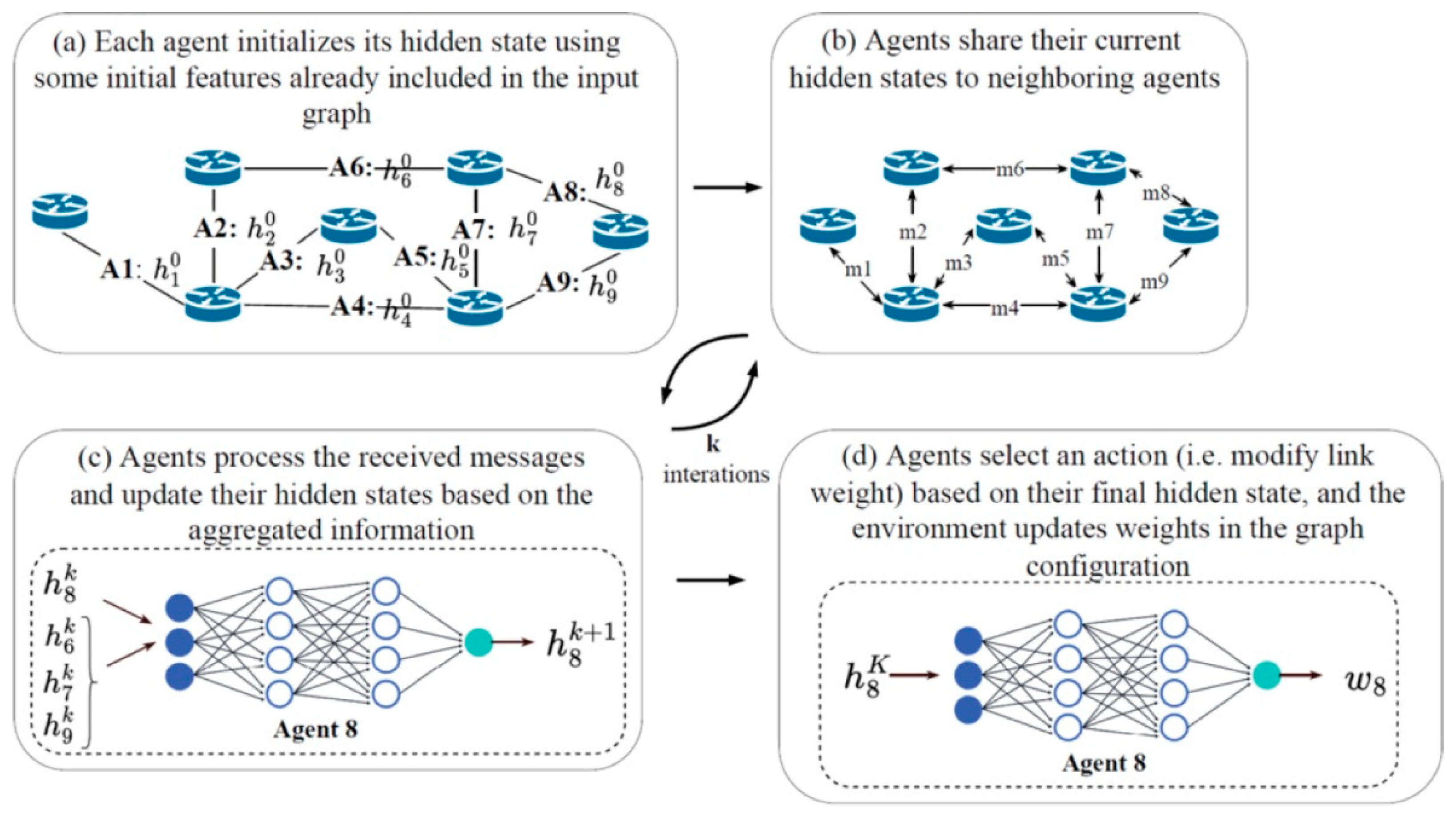
As mentioned earlier, the developed method is based on MAROH. Here, a brief description of MAROH is provided, necessary for understanding the new method. In MAROH each agent manages one channel and calculates the weight of its channel to achieve uniform channel loading (see Figure 1). Uniformity is ensured by multi-agent optimization of the functional Φ that is value of the channel load deviation from the average network load:
where is the occupied channel bandwidth, is the nominal channel bandwidth and is the average channel load in the network.
Balancing consists of distributing data flows proportionally to channel weights. This way makes the agent operation to be independent of the number of channels on a network device. The agent state is a pair of channel weight and channel load (Figure 1(a)). Each agent, upon changing its state (called a hidden state), transmits its state to the agent neighbors (Figure 1(b)). Neighbors are agents on adjacent nodes in the network topology. Each agent processes the received hidden states from neighbors using a graph neural network that is Message Passing Neural Network (MPNN). The collected hidden states are processed by the agent’s special neural network, referred to as "update," which calculates the agent's new hidden state (Figure 1(c)). This process is repeated K times. The value of K determines the size of agent neighborhood domain, i.e., how many states of other agents are involved into calculation of the current hidden state. K is a method parameter. After K iterations, the resulting hidden state is fed into a special neural network, referred to as "readout". Outputs of readout network are used to select an action for weight adjustment by the softmax function. On Figure 1(d) it is shown the readout neural network operation finishing with a new weight. The steps of action selection are omitted there. Possible actions for weight calculation include:
- Addition: +1;
- Null action: +0;
- Mulitplication: *k (k is a tunable parameter);
- Division: /k (k is a tunable parameter).
Figure 1.
Schematic of the MAROH method [5].
Figure 1.
Schematic of the MAROH method [5].
MAROH agents update weights not upon the arrival of each new flow but only when the channel load changing exceeds a specified threshold. In this way, feedback on channel load fluctuations is regulated, which minimizes the overhead of the agent's operation. New flows are distributed according to the current set of weights without delay for agent decisions. However, outdated weights may lead to suboptimal channel loading, so it is crucial for agents in the proposed method to decide on weight adjustments as quickly as possible.
4. Proposed Methods
This section presents solutions that allow agents to operate independently and transform the agent control plane into two-layer one.
4.1. Simultaneous Actions MAROH (SAMAROH)
Let’s introduce some terms. The time interval between agent hidden state initialization and action selection is called a horizon. For an agent, a new horizon begins when the channel load changes beyond a specified threshold. An episode is a fixed number of horizons required for the agent to establish the optimal channel weight. The limitation (only one agent acting) in MAROH was introduced for theoretical justification of its convergence. However, experiments showed that convergence to the optimal solution persists even with asynchronous agent actions.
Let us consider the number of horizons required to achieve optimal weights by MAROH and by simultaneously acting agents. Let { is the set of optimal weights. For simplicity, suppose the agents are allowed to do as action only to add one to the weight (consideration with other actions is similar). In this case, MAROH will take actions (and thus horizons) to achieve optimal weights. When agents operate independently, they only need horizons. Therefore, independent agents operating can significantly reduce the time to get the optimal weights and reduce number of horizons. For example, for a rhombus topology with 8 agents, about 100 horizons are needed, but 20 is enough in case of independent agent operating.
In the new approach called SAMAROH (Simultaneous Actions MAROH), all agents can independently adjust weights in each of their horizons. To simplify convergence, following [11], the number of agent actions was reduced to:
- Multiplication: *k (k is a tunable parameter);
- Null action: +0.
In MAROH, agents at each horizon selected a single agent and the action it would perform. This occurred as follows: each agent collected a vector of readout neural network outputs from all other agents and applied the softmax function to select the best action. In SAMAROH, the agent collects only a local vector with the readout output for each action, further reducing inter-agent exchanges. Unlike [11], where the number of acting agents was restricted by a constant, our approach allows all agents to act independently. Experimental results (see Section 6) show this does not affect the method's accuracy.
4.2. Two-Layers Control Plane MAROH (MAROH-2L)
The second innovation, based on [6], divides the control plane into two layers: experience and decision-making, detailed below.
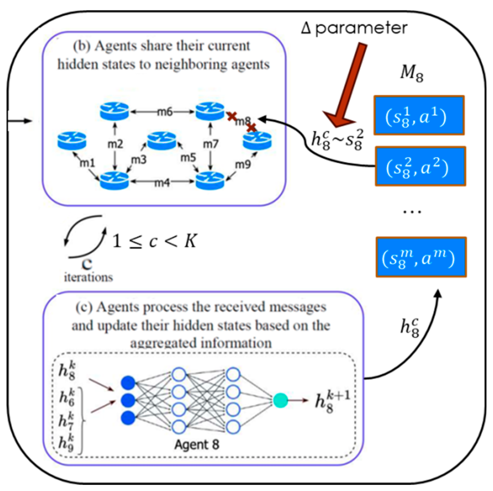
4.2.1. Experience Layer
Each agent stores past hidden states and corresponding actions. Their collection is called the agent's memory. Denote the memory of the i-th agent as :
, where is the hidden state of agent i before the (+1)-th exchange iteration, is the memory size (number of stored states), is the number of agents in the system, is the maximum number of exchange iterations, and is the action taken by the agent after completing K exchange iterations.
When assessing how close the current state is to familiar states, the agent takes into account all past hidden states at all intermediate iterations of the exchange in MPNN (l∈{1,…,K-1}). This allows familiar states to be identified during the progression toward the horizon.
The second component of a memory element is the agent action, taken after the final K-th exchange iteration. However, it is possible to store the input or output of the readout network, that let reconstruct the selected action. In this case, an ε-greedy strategy can be applied to the agent's decision-making process to improve learning efficiency [12], and the readout network can be further trained.
Figure 2.
Schematic of the experience layer operation for the eighth agent.
Let call a case as a possible memory element. Denote be the set of all cases, i.e., possible memory elements that may arise for an agent. Let Δ: , called the threshold. Denote as the metric on , where . Recall that is symmetric, non-negative, and satisfies the triangle inequality. If , and are called close. A case is familiar to i-th agent if .
Hidden states are vectors resulting from neural network transformations. The components of vector h = (h₁,...,hᴰ) are numerical representations obtained through nonlinear neural network transformations without direct interpretable meaning. The dimensionality D of the hidden state does not have significant importance. It directly affects the volume of messages exchanged between agents, as each message size linearly depends on D. Moreover, the choice of a value of D allows balancing the trade-off between the objective function's value and network load. As it was shown in [5] that increasing of D generally improves balancing quality but increases the overhead.
To measure the distance between vectors on the experience layer, the following three metrics were used:
- Euclidean metric (L2):
- 2.
- Manhattan metric (L1):
- 3.
- Cosine distance1 (Cos):
These metrics were chosen due to the equal significance of hidden state vector components and low computational complexity. Their comparative analysis is detailed in Section 6.
Since the agent's memory size is limited, it only includes hidden states called representatives. The choice of representatives is discussed in Section 4.2.2 and Section 4.2.3. Although is considered as prefixed in this paper, the two-layer method could be generalized to the case that is specific for each representative. The value of is the parameter balancing the trade-off between the number of transmitted messages (i.e., how many close states are detected) and solution quality. Each metric requires individual threshold tuning.
Depending on the method for selecting representative for hiden states, there may be alternative when for the same hidden state either there is a single representative (Section 4.2.3) or there are multiple representatives (Section 4.2.2). In the latter, the agent selects the representative with the minimal distance .
There may be cases where the agent memory stores suboptimal actions, as agents are not fully trained or employ an ε-greedy strategy [12]. Therefore, in the two-layer method, when a representative is found, an additional parameter is used to determine the probability of transition to the experience layer. That is, with a certain probability, the agent may start interacting with other agents to improve its action selection, even if a representative for the current state exists in memory.
4.2.2. Decision-Making Layer
At the decision-making layer, the agent, by communicating with other agents, selects an action for a new, unfamiliar state, as in MAROH. At this layer, the agent enriches its memory by adding a new representative. Recall that the agent's memory stores not all familiar cases but their representatives. There were explored two ways to determine representatives: experimentally, based on clustering methods, and theoretically, based on constructing an -net [15]2. Let be the threshold—the metric value beyond which a state is considered unfamiliar.
Consider the process of selecting memory representatives based on clustering. It is clear that clustering is computationally more complex than -net way, and does not guarantee a single representative for a state.
Initially, when memory is empty, all hidden states are stored until memory is exhausted. The hidden states are added to memory upon the MPNN message processing cycle complete and actions are known.
Any state without a representative in memory is a new candidate for representation. To avoid heavy clustering for each new candidate, they are gathered in a special array . Once this array is full, joint clustering of arrays and into clusters is performed. After clustering, candidates and existing representatives are merged into clusters by metric , leaving one random state per cluster as the memory representative. Thus, after clustering, selected states remain in , and is cleared. Several clustering algorithms can be used to find representatives. In [9], Mini-Batch K-Means showed the best performance in terms of complexity and message volume. However, since this algorithm only works with (2), Agglomerative Clustering [16] was used for other metrics.
The clustering algorithm with minimal complexity is Mini-Batch K-Means. Its complexity is at least , where is the batch size, is the number of clusters, is data dimensionality, and is the number of iterations. Such complexity may be unacceptable for large-scale networks. Section 4.2.3 proposes an alternative method eliminating clustering, reducing complexity to using Δ-nets [15].
4.2.3. Decision-Making Layer: -Net Based Method
This section describes the representative selection algorithm based on -nets [15] and its theoretical justification. It is simpler and avoids computationally intensive clustering.
Let be a finite set of cases. Randomly select . For any such that is considered the representative of . The representatives are denoted as , and their set as . To get a unique representative for any case the the condition must hold.
Representative Selection Method: Let . For each new element from , searching in for such, that , where is arbitrarily small known in advance. If such exists, it is accepted as the representative for .
If no such exists in , find in , minimizing . Let .
If , declare a temporary representative and form , but .
Next, search for temporary representative , where , but
and replace with in , declaring it the new temporary representative . This process is repeated until . Because we are working in a metric space and - the set of agent states is finite, the process will complete at some time t, and -net [15] is obtained. If is non-empty, temporary representatives will have overlapping -net regions with representatives. For these overlaps, assign them to a representative, e.g., only representatives with the same action as the new case.
If , then declare a representative and remove all temporary from such that .
This part of the representative selection procedure constitutes the essence of the decision-making layer.
This procedure ensures:
- Either or . In the last alternative the chois is made based on the coincidence of actions in If the actions are coincedented in these cases, then the choice is random.
This proposition holds true by construction of the representative selection algorithm.
The computational complexity of Δ-net based method is arithmetic operations for comparing a new hidden state (a d-dimensional vector) with each representative.
The two-layer control plane applies to both SAMAROH and MAROH. Their modifications are denoted SAMAROH-2L and MAROH-2L, respectively.
5. Materials and Methods
All algorithms of the proposed methods were implemented in Python with TensorFlow framework and are publicly available on GitHub [17]. The code is in the dte_stand directory. Input data for the experiments (Section 6 results) are in data_examples directory. Each experiment input included:
- network topology;
- load as traffic matrix;
- balancing algorithm and its parameters (memory size, threshold Δ, metric, clustering algorithm).
Taking into consideration the computational complexity of multi-agent methods, experiments were restricted by four topologies. Two (Figure 3) were synthetic and symmetric for transparency of demonstration. The symmetry was used for debugging purposes - under uniform load conditions the method was expected to produce identical weights, while under uneven channel loads the resulting weights were expected to balance the load distributions. Other topologies were taken from TopologyZoo [18], selected for ≤100 agents (for computational feasibility with the constraint of no more than one week per experiment) and maximal alternative routes. All channels were bidirectional with equal capacity.
Figure 3.
Symmetric topologies for experiments: (a) 4-node with 8 agents; (b) 16-node with 64 agents.
Figure 3.
Symmetric topologies for experiments: (a) 4-node with 8 agents; (b) 16-node with 64 agents.
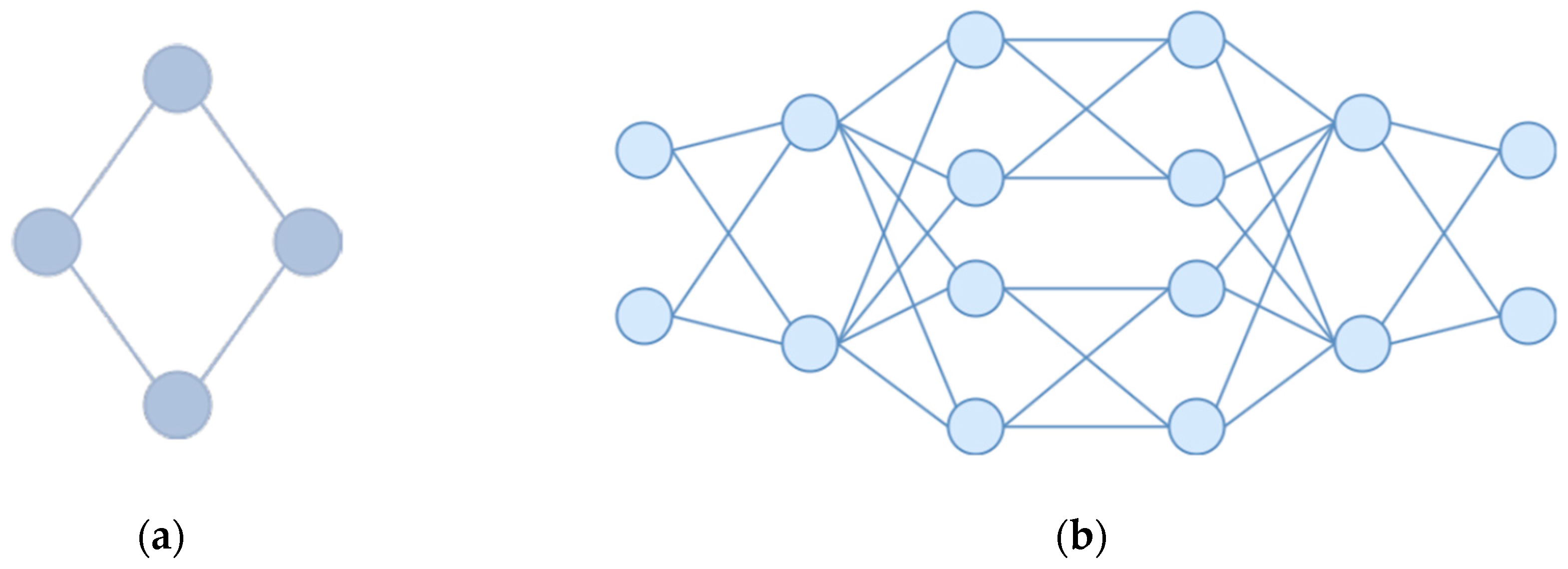
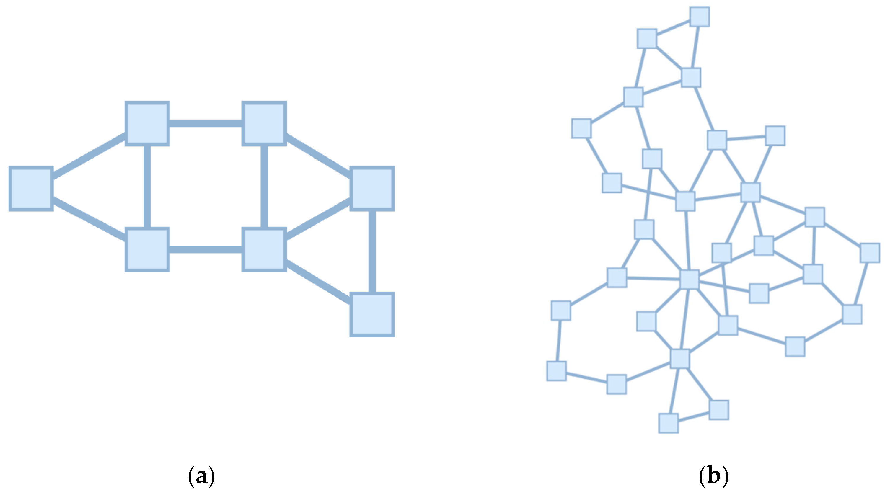
Figure 4.
Topologies from the TopologyZoo library: (a) Abilene - modified to reduce the number of transit vertices while preserving the asymmetry of the original topology. The final configuration contains 7 nodes and 20 agents; (b) Geant2009 - with degree-1 vertices removed. The final configuration consists of 30 nodes and 96 agents.
Network load was represented by the set of flows, each as the tuple (source, destination, rate, start/end time) and the scheduling of their beginings. Flows were generated for average network loads of 40% or 60%.
The investigated algorithms and their parameters were specified in tabular form (for details, see the following section).
Results were evaluated based on the objective function Φ (1) (also called solution quality) and the total number of agent exchanges.
To evaluate the obtained optimality of solutions the results of experiments were compared with those of the centralized genetic algorithm. Although the genetic algorithm provided an approximate suboptimal solution to the NP-complete balancing problem—unlike the proposed method, it relied on a centralized view of all channel states—the values obtained through the genetic algorithm served as our benchmark.
The genetic algorithm with the objective to minimize the target function Φ was organized as follows. The crossover operation between two solutions (i.e., two sets of agent weights) worked as follows: over several iterations, Solution 1 and Solution 2 exchanged the weights of all agents at a randomly selected network node. The mutation operation involved multiple iterations where the weights of all agents at a randomly chosen node were cyclically shifted, followed by the reinitialization of a randomly selected subset of these weights with new random values. Solution selection was performed based on the value of the objective function Φ.
For simplicity of the experiments the synchronous switching of all agents between layers were used. If any single agent failed to identify sufficiently similar states in its memory, it is assumed to trigger a cascade transition to the decision-making layer: first, its immediate neighbors would activate this layer, followed by their neighbors in turn, propagating through the network until all agents had switched to the decision-making layer.
6. Experimental Results
6.1. MAROH vs SAMAROH
In the first series of experiments the effectiveness of simultaneous weight adjustments by all agents compared with sequential one where only a single agent performs actions. In Figure 5 and Figure 6 the comparison between MAROH and SAMAROH methods for (a) the 4-node topology (Figure 3a) and (b) Abilene topology (Figure 4a) under different load conditions is exibite. On these figures solid lines represent the average Φ values over 100-episode intervals, while semi-transparent shaded areas of corresponding colors indicate the range from minimum to maximum Φ values across these 100-episode blocks. Colored asterisks mark the minimum values of Φ averaged over 2000-episode intervals.
In Figure 5 and Figure 6, the green line representing SAMAROH's objective function values consistently remains below the blue one corresponding to MAROH's performance. This fenomen demonstrates that despite all agents acting simultaneously, SAMAROH not only keep but actually get better quality solution. This can be explained by the fact that agents need to be trained to act in fewer horizons during an episode, which simplifies the training.
These figures also represent the results obtained with uniformed weights, representing traditional load-balancing approaches like ECMP. As evident across all plots, the green line (SAMAROH) consistently shows closer alignment with the centralized algorithm's performance (indicated by a dark green solid horizontal line) compared to the gray dashed line representing ECMP.
SAMAROH employed five times fewer horizons than the original MAROH (20 vs. 100 for the 4-node topology and 50 vs. 250 for Abilene). This translates to a fivefold reduction in both inter-agent communications and decision-making time, as achieving comparable results now requires significantly fewer horizons.
6.2. Research of Two-Layer Approach
The next series of experiments were dadicated to evaluating of the efficiency of the two-layer approach was evaluated. Figure 7 and Figure 8 present the comparing this approach across all topologies, benchmarking the method against SAMAROH, the centralized genetic algorithm, and ECMP. In the legend, the two-layer method agent communication count (shown in parentheses) is expressed relative to SAMAROH's baseline exchange volume.
In Figure 7 and Figure 8, the objective function values for SAMAROH-2L (shown as blue and green lines for different proximity thresholds) consistently match or fall below the yellow line corresponding to SAMAROH's performance. The only exception is Figure 8a, where the blue line exceeds the yellow one. However, the plot clearly shows the blue line's downward trend, suggesting values would likely converge given more training episodes.
The general conclusion from these results is as following: with a moderate reduction in message exchanges (up to 20% for the Abilene topology, Figure 8a), the two-layer method achieves objective function values that slightly differ from SAMAROH ones. With more substantial reductions in exchanges, the two-layer method either yields significantly worse solution quality (for the Abilene topology, Figure 8a) or requires more training episodes to match SAMAROH's performance (for the 4-node topology, Figure 7a). Meanwhile, the actual reduction in inter-agent exchanges can be adjusted between 25-50% depending on the required solution accuracy.
Figure 8(a) demonstrates that the proximity threshold Δ has significant impacts as on the objective function value as on the number of inter-agent exchanges. Furthermore, the two-layer method's performance has also under influence of two key parameters: memory size and the comparison metric employed. The corresponding series of the experiments systematically evaluates the method efficacy across varying configurations of these parameters (see Table 1, Table 2 and Table 3).
Figure 7.
Dependence of the objective function value on the episode number under 40% load for symmetric topologies: (a) 4-node with 8 agents; (b) 16-node with 64 agents.
Figure 7.
Dependence of the objective function value on the episode number under 40% load for symmetric topologies: (a) 4-node with 8 agents; (b) 16-node with 64 agents.
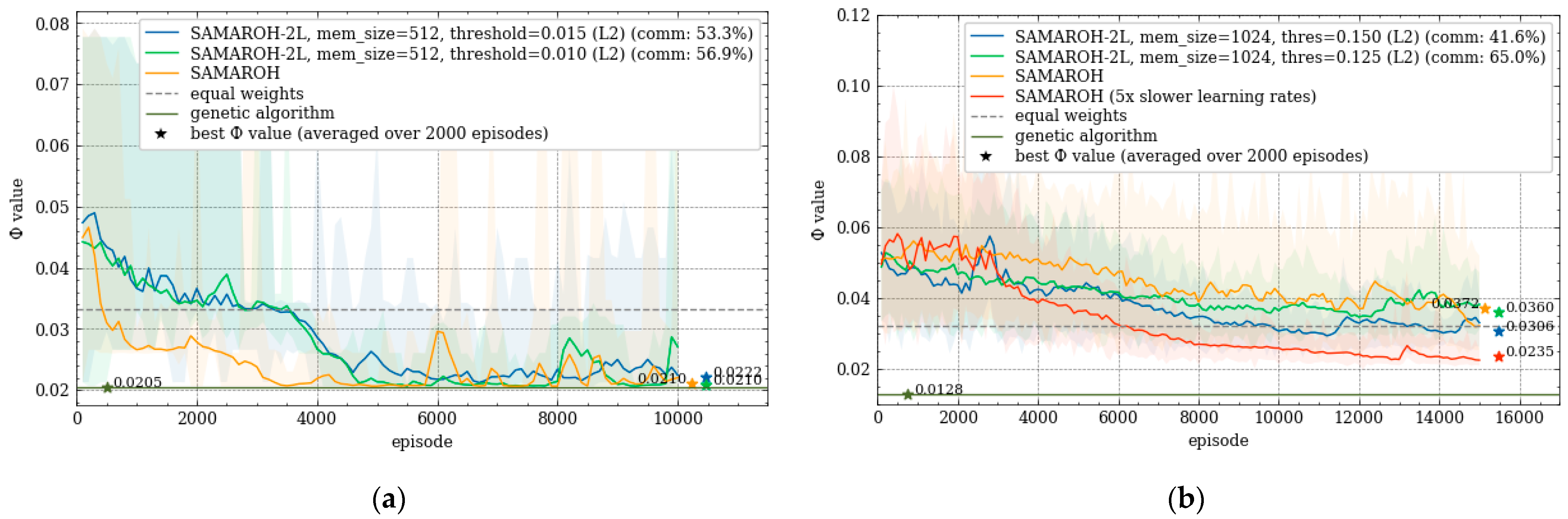
Figure 8.
Dependence of the objective function value on the episode number under 40% load for c topologies from TopologyZoo Library: (a) Abilene; (b) Geant2009.
Figure 8.
Dependence of the objective function value on the episode number under 40% load for c topologies from TopologyZoo Library: (a) Abilene; (b) Geant2009.
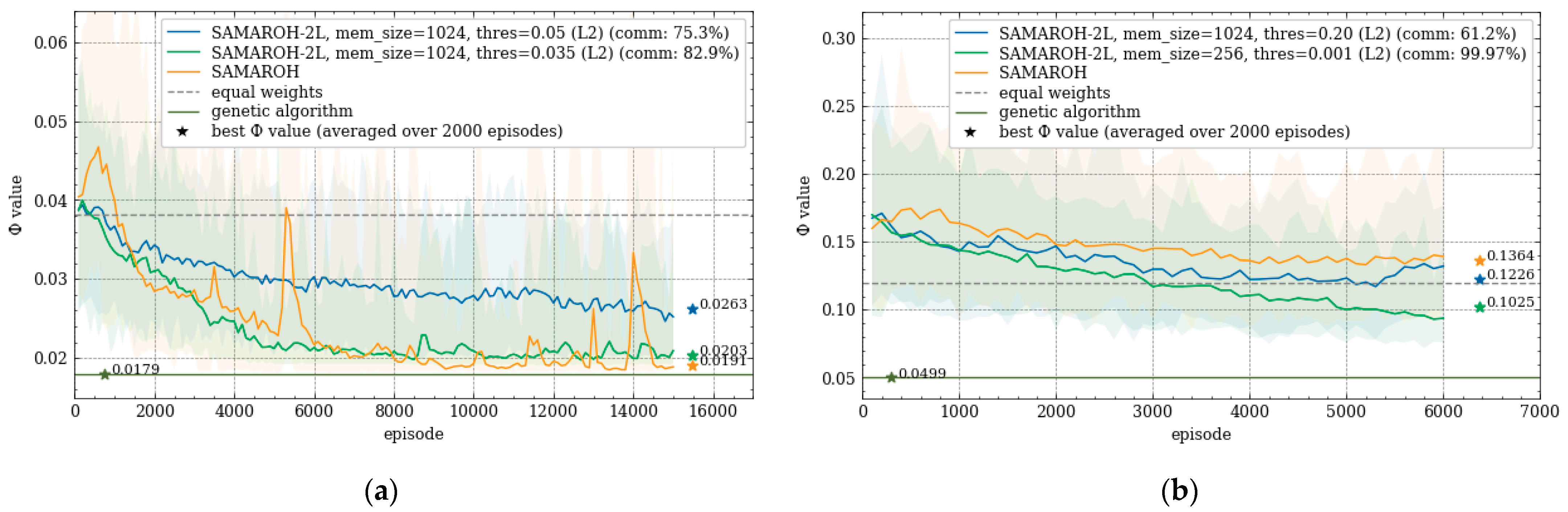
Table 1 presents a comparison of the objective function values and exchange counts for the symmetric 4-node topology under 40% load, while Table 2 and Table 3 show corresponding data for the Abilene topology at the same load level. Each reported value represents an average across 2 experimental runs. Due to computational constraints (with a single experiment involving 96 agents requiring over a week to complete) comprehensive parameter comparisons were not conducted for larger topologies. The Φ values shown in the tables correspond to the minimum averaged values computed over 2000-episode intervals.
For the 4-node topology, the memory size was fixed at 512 states based on the results from [9], representing the maximum capacity we could use to store representatives. As shown in Table 1, Φ values remain relatively stable at small threshold values, but the objective function begins to degrade as the threshold grouth. This pattern is completely corresponded to the one in the Abilene topology results (Table 2 and Table 3). This is explained by the fact that with increasing threshold, states that correspond to different actions become close however the agent will apply the same action in both states. In the conducted series of experiments, the threshold value was set manually, but the question arises about an automatic method for selecting the value of this parameter in such a way that the compromise between the value of the objective function and the number of exchanges is observed.
The metric comparison across Table 1, Table 2 and Table 3 revealed that the L2 metric achieves superior solution quality under the same number of echanges.
For the Abilene topology, the memory size was set to 512 states (Table 2), consistent with configuration in [9] for a comparable 4-node topology with similar agent number. Increasing the memory capacity to 1024 states (Table 3) while maintaining the same threshold has led to downgrade of the objective. This can be explained by the fact that a larger number of representatives will have an intersection of Δ-neighborhoods that can have different actions, which justifies the relevance of the method for selecting representatives without intersection of Δ-neighborhoods proposed in section 4.2.3.
A comparison between MAROH-2L and SAMAROH-2L in Table 1 reveals that while using identical memory parameters, SAMAROH-2L achieves a 40-70% reduction in message exchanges, whereas MAROH-2L only attains a 4-9% reduction. This performance gap likely stems from MAROH-2L's fivefold greater number of horizons per episode, which generates proportionally more hidden states - consequently, the same memory size proves inadequate compared to SAMAROH-2L's requirements.
In Table 1, Table 2 and Table 3 the number of exchanges between agents is given as a percentage in relation to the number of exchanges in the SAMAROH method. If we take into account the reduction in the number of horizons in one episode, then the reduction in the number of exchanges will be much more significant. Thus, for Table 3 the number of horizons in one episode was reduced by 5 times, therefore the reduction, for example, to 69.43% actually means that it was reduced to 100/5*0.8071≈16.14%. In conclusion, the two-layer SAMAROH-2L method achieved significant improvements: for the 8-agent topology, it reduced the objective function value to 0.0215 while cutting communication exchanges by 37.02% (from 100% to 62.98% relative to SAMAROH baseline), and for the Abilene topology, it maintained near-optimal performance with only a 0.0014 increase in the objective function (from 0.0196 to 0.0210) alongside a 19.29% reduction in exchanges (from 100% to 80.71%).
7. Discussion
The efficiency of the proposed two-layer method was experimentally proved. This is especially clearly visible from the experiments with Abilene topology, the method maintained high-quality solutions (with the objective function changing only from 0.0196 to 0.0210) while achieving a 19.29% reduction in communication volume.
Promising directions for future research include:
- investigating the effectiveness of the representative selection method proposed in Section 4.2.3;
- developing adaptive algorithms for states proximity threshold tuning;
- creating dynamic memory management techniques with intelligent identification of obsolete states and optimal memory sizing based on current network conditions;
- optimizing computational complexity for large-scale network topologies.
The current limitations of the method primarily involve extended training durations for 96-agent systems (necessitating distributed simulation frameworks) and the substantial number of required training episodes (4,000-10,000). While accelerating multi-agent methods was not this study's primary focus, it remains a crucial direction for future research.
It is particularly noteworthy that the proposed two-layer approach, while developed for traffic flow balancing, demonstrates universal applicability and can be adapted to a broad class of cooperative multi-agent systems where agents collaboratively solve shared tasks.
8. Conclusions
A new multi-agent method for traffic flow balancing is presented, based on two fundamental innovations: abandoning sequential models of agent decision making and developing a two-layer human-like agent control plane in multi-agent optimization. For the agent control plane, a concept of agent hidden states representative reflecting its experience was proposed. This concept has allowed to significantly reduce the number of stored hidden states. Two methods of representative selecting were proposed and investigated. Experimentally was proven that proposed innovations let significantly reduce the amount of inter-agent communications, decision making time by agents and optimality of flow balancing while maintaining the original objective function.
Author Contributions
E.S.: methodology, project administration, software, writing—original draft, validation. R.S.: methodology, conceptualization, writing—review and editing, supervision. I.G.: software, investigation, visualization, formal analysis. All authors have read and agreed to the published version of the manuscript.
Funding
This work was supported by the The Ministry of Economic Development of the Russian Federation in accordance with the subsidy agreement (agreement identifier 000000C313925P4H0002; grant No 139-15-2025-012).
Data Availability Statement
Source code and experiment input data available at https://github.com/estepanov-lvk/maroh.
Acknowledgments
We acknowledge graduate student Ariy Okonishnikov for his contributions to the initial implementation and preliminary experimental validation of the method.
Conflicts of Interest
The authors declare no conflicts of interest.
Abbreviations
The following abbreviations are used in this manuscript:
| ECMP | Equal-Cost Multi-Path |
| MAROH | Multi-Agent ROuting using Hashing |
| MAROH-2L | MAROH with Two-Layer Control Plane |
| MPNN | Message Passing Neural Network |
| NP | Non-deterministic Polynomial time |
| RL | Reinforcement Learning |
| SAMAROH | Simultaneous Actions MAROH |
| UCMP | Unequal-Cost Multi-Path |
References
- Moiseev N.N., Ivanilov Yu.P., Stolyarova E.M. (1978) Optimization methods. Moscow: Nauka. 352 p.
- Wang, I-Lin. "Multicommodity network flows: A survey, Part I: Applications and Formulations." International Journal of Operations Research 15, no. 4 (2018): 145-153. [CrossRef]
- Wang, I-Lin. "Multicommodity network flows: A survey, part II: Solution methods." International Journal of Operations Research 15, no. 4 (2018): 155-173. [CrossRef]
- Even, Shimon, Alon Itai, and Adi Shamir. "On the complexity of time table and multi-commodity flow problems." 16th annual symposium on foundations of computer science (sfcs 1975). IEEE, 1975. [CrossRef]
- Stepanov, E. P., R. L. Smeliansky, A. V. Plakunov, A. V. Borisov, Xia Zhu, Jianing Pei, and Zhen Yao. "On fair traffic allocation and efficient utilization of network resources based on MARL." Computer Networks 250 (2024): 110540. [CrossRef]
- Kahneman, Daniel. Thinking, fast and slow. macmillan, 2011.
- Ramani, Dhruv. "A short survey on memory based reinforcement learning." arXiv preprint arXiv:1904.06736 (2019). [CrossRef]
- Zheng, Lulu, Jiarui Chen, Jianhao Wang, Jiamin He, Yujing Hu, Yingfeng Chen, Changjie Fan, Yang Gao, and Chongjie Zhang. "Episodic multi-agent reinforcement learning with curiosity-driven exploration." Advances in Neural Information Processing Systems 34 (2021): 3757-3769. [CrossRef]
- Okonishnikov, A. A., and E. P. Stepanov. "Memory mechanism efficiency analysis in multi-agent reinforcement learning applied to traffic engineering." 2024 International Scientific and Technical Conference Modern Computer Network Technologies (MoNeTeC). IEEE, 2024. [CrossRef]
- Yao, Z., Ding, Z. and Clausen, T., 2022, October. Multi-agent reinforcement learning for network load balancing in data center. In Proceedings of the 31st ACM International Conference on Information & Knowledge Management (pp. 3594-3603). [CrossRef]
- Bernárdez, Guillermo, José Suárez-Varela, Albert López, Xiang Shi, Shihan Xiao, Xiangle Cheng, Pere Barlet-Ros, and Albert Cabellos-Aparicio. "MAGNNETO: A graph neural network-based multi-agent system for traffic engineering." IEEE Transactions on Cognitive Communications and Networking 9, no. 2 (2023): 494-506. [CrossRef]
- Sutton, Richard S., and Andrew G. Barto. Reinforcement learning: An introduction. Vol. 1, no. 1. Cambridge: MIT press, 1998.
- Kryszkiewicz, Marzena. "The cosine similarity in terms of the euclidean distance." In Encyclopedia of Business Analytics and Optimization, pp. 2498-2508. IGI Global, 2014. [CrossRef]
- Xia, Peipei, Li Zhang, and Fanzhang Li. "Learning similarity with cosine similarity ensemble." Information sciences 307 (2015): 39-52. [CrossRef]
- Yosida, Kôsaku. Functional analysis. Vol. 123. Springer Science & Business Media, 2012.
- Overview of clustering methods. Available online: https://scikit-learn.org/stable/modules/clustering.html#overviewof-clustering-methods (accessed on 05 August 2025).
- MAROH implementation. Available online: https://github.com/estepanov-lvk/maroh.git (accessed on 05 August 2025).
- Topology zoo. Available online: https://github.com/sk2/topologyzoo (accessed on 31 July 2025).
Figure 5.
Dependence of the objective function value on the episode number for MAROH and SAMAROH methods under 40% load for: (a) 4-node topology; (b) Abilene topology.
Figure 5.
Dependence of the objective function value on the episode number for MAROH and SAMAROH methods under 40% load for: (a) 4-node topology; (b) Abilene topology.
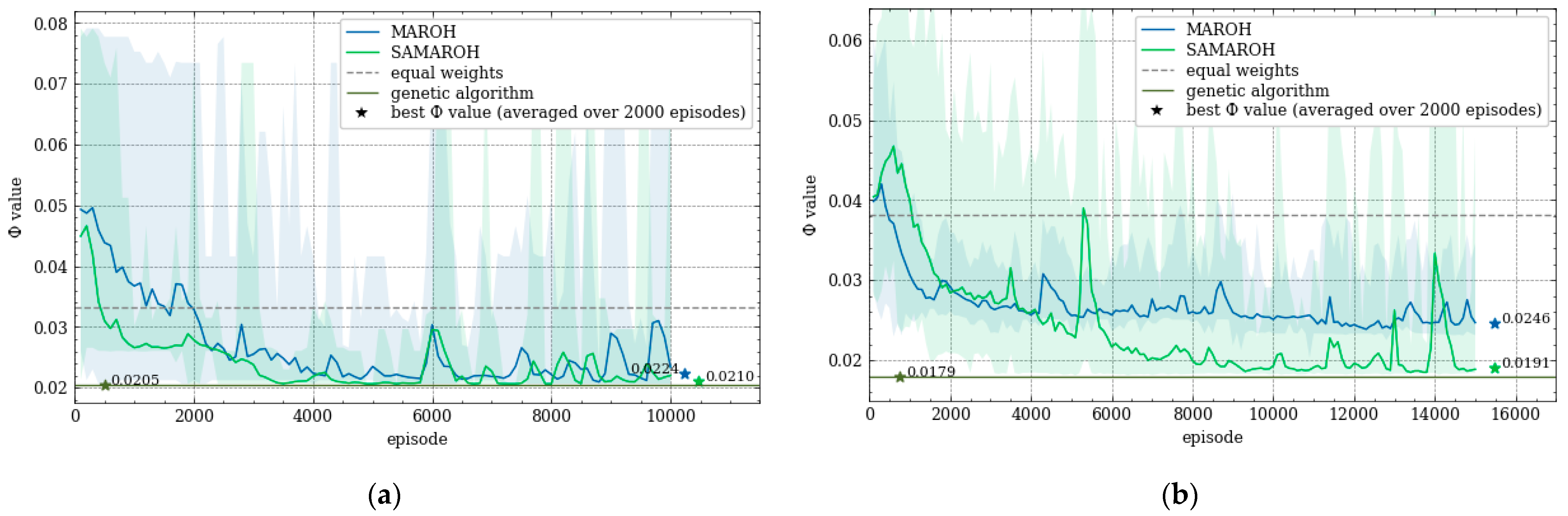
Figure 6.
Dependence of the objective function value on the episode number for MAROH and SAMAROH methods under 60% load for: (a) 4-node topology; (b) Abilene topology.
Figure 6.
Dependence of the objective function value on the episode number for MAROH and SAMAROH methods under 60% load for: (a) 4-node topology; (b) Abilene topology.
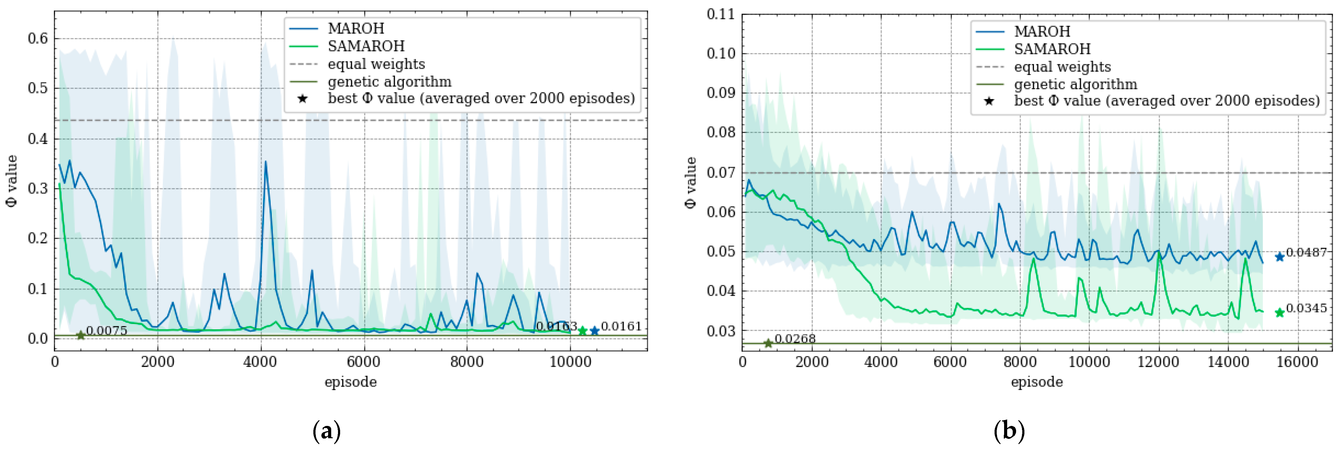

Table 1.
Experimental comparison results of the proposed methods for the 4-node topology with 8 agents over 6000 episodes.
Table 1.
Experimental comparison results of the proposed methods for the 4-node topology with 8 agents over 6000 episodes.
| Algorithm | Clustering | Metric | Memory size | Threshold | Φ | Number of exchanges (%) |
|---|---|---|---|---|---|---|
| Genetic | - | - | - | - | 0.0205 | - |
| MAROH | - | - | 0 | - | 0.0280 | 100.00% |
| SAMAROH | - | - | 0 | - | 0.0231 | 100.00% |
| MAROH-2L | MiniBatch KMeans | L2 | 512 | 0.007 | 0.0249 | 95.86% |
| 0.010 | 0.0225 | 91.56% | ||||
| 0.015 | 0.0229 | 93.57% | ||||
| 0.018 | 0.0247 | 94.28% | ||||
| 0.025 | 0.0229 | 87.29% | ||||
| 0.030 | 0.0230 | 75.52% | ||||
| 0.040 | 0.0246 | 57.45% | ||||
| 0.050 | 0.0259 | 60.57% | ||||
| 0.060 | 0.0258 | 60.52% | ||||
| 0.070 | 0.0259 | 43.98% | ||||
| SAMAROH-2L | MiniBatch KMeans | L2 | 512 | 0.007 | 0.0256 | 62.29% |
| 0.010 | 0.0215 | 62.98% | ||||
| 0.015 | 0.0236 | 51.13% | ||||
| 0.018 | 0.0284 | 27.46% | ||||
| Agglomerative Clustering | L1 | 512 | 0.01 | 0.0211 | 87.80% | |
| 0.03 | 0.0278 | 75.81% | ||||
| 0.04 | 0.0290 | 50.95% | ||||
| 0.05 | 0.0286 | 30.20% | ||||
| Cos | 512 | 1e-7 | 0.0257 | 77.67% | ||
| 3e-7 | 0.0261 | 76.92% | ||||
| 4e-7 | 0.0272 | 47.68% | ||||
| 5e-7 | 0.0293 | 60.04% |
Table 2.
Experimental comparison results of the proposed methods for Abilene topology with 512 memory size over 15000 episodes.
Table 2.
Experimental comparison results of the proposed methods for Abilene topology with 512 memory size over 15000 episodes.
| Algorithm | Clustering | Metric | Memory size | Threshold | Φ | Number of exchanges (%) |
|---|---|---|---|---|---|---|
| Genetic | - | - | - | - | 0.0179 | - |
| MAROH | - | - | 0 | - | 0.0247 | 100.00% |
| SAMAROH | - | - | 0 | - | 0.0196 | 100.00% |
| SAMAROH-2L | MiniBatch KMeans | L2 | 512 | 0.035 | 0.0227 | 91.44% |
| 0.040 | 0.0187 | 88.73% | ||||
| 0.050 | 0.0211 | 84.13% | ||||
| 0.060 | 0.0210 | 80.71% | ||||
| Agglomerative Clustering | L1 | 512 | 0.052 | 0.0220 | 99.93% | |
| 0.062 | 0.0190 | 99.37% | ||||
| 0.067 | 0.0224 | 99.06% | ||||
| 0.077 | 0.0215 | 97.17% | ||||
| Cos | 512 | 1.5e-7 | 0.0234 | 98.61% | ||
| 3e-7 | 0.0205 | 98.48% | ||||
| 4.5e-7 | 0.0209 | 98.22% | ||||
| 7.5e-7 | 0.0218 | 97.67% |
Table 3.
Experimental comparison results of the proposed methods for Abilene topology with 1024 memory size over 15000 episodes.
Table 3.
Experimental comparison results of the proposed methods for Abilene topology with 1024 memory size over 15000 episodes.
| Algorithm | Clustering | Metric | Memory size | Threshold | Φ | Number of exchanges (%) |
|---|---|---|---|---|---|---|
| Genetic | - | - | - | - | 0.0179 | - |
| MAROH | - | - | 0 | - | 0.0247 | 100.00% |
| SAMAROH | - | - | 0 | - | 0.0196 | 100.00% |
| SAMAROH-2L | MiniBatch KMeans | L2 | 1024 | 0.035 | 0.0211 | 82.26% |
| 0.040 | 0.0214 | 82.61% | ||||
| 0.050 | 0.0226 | 69.43% | ||||
| 0.060 | 0.0320 | 53.32% | ||||
| Agglomerative Clustering | L1 | 1024 | 0.052 | 0.0208 | 96.10% | |
| 0.062 | 0.0214 | 88.81% | ||||
| 0.067 | 0.0214 | 82.85% | ||||
| 0.077 | 0.0294 | 57.93% | ||||
| Cos | 1024 | 1.5e-7 | 0.0234 | 95.70% | ||
| 3e-7 | 0.0207 | 89.44% | ||||
| 4.5e-7 | 0.0225 | 74.05% | ||||
| 7.5e-7 | 0.0303 | 37.12% |
| 1 | It should be noted that cosine distance is not formally a metric, as it does not satisfy the triangle inequality. Nevertheless, as shown in [13], the problem of determining a cosine similarity neighborhood can be transformed into the problem of determining the Euclidean distance, and cosine distance is widely used in machine learning [14]. |
| 2 | An ε-net is a subset Z of a metric space X for such that that is no farther than ε from x. Since we are working in a metric space and the set of agent states is finite, an ε-net exists for it. |
Disclaimer/Publisher’s Note: The statements, opinions and data contained in all publications are solely those of the individual author(s) and contributor(s) and not of MDPI and/or the editor(s). MDPI and/or the editor(s) disclaim responsibility for any injury to people or property resulting from any ideas, methods, instructions or products referred to in the content. |
© 2025 by the authors. Licensee MDPI, Basel, Switzerland. This article is an open access article distributed under the terms and conditions of the Creative Commons Attribution (CC BY) license (https://creativecommons.org/licenses/by/4.0/).
Copyright: This open access article is published under a Creative Commons CC BY 4.0 license, which permit the free download, distribution, and reuse, provided that the author and preprint are cited in any reuse.


