1. Introduction
Traffic congestion is becoming an increasingly critical issue in medium to large cities, affecting the quality of life for citizens [
1].
A primary factor contributing to traffic congestion is the surge in population growth. As the population increases, so does the number of vehicles on the road. According to the United Nations, 54% of the world’s population resides in urban areas, and this percentage is expected to rise to 66% by 2050 [
2]. This growth directly correlates with increased traffic congestion [
2]. As cities continue to expand, the layout of intersections can become increasingly complex. Most blocks can only accommodate a limited amount of vehicles at a stoplight before traffic gets backed up. In densely populated conditions, traffic congestion is exacerbated by narrow road widths, limited vehicle parking, traffic signals and maintenance operations [
3]. Global warming, which directly influences wind patterns, rainfall, and other extreme atmospheric events, plays a significant role in accelerating the deterioration of pavement conditions. This environmental phenomenon is not only a contributing factor to the degradation of our city infrastructures but also a consequence of it. The interplay between global warming and deteriorating pavement conditions forms a complex cycle that exacerbates both traffic congestion and environmental issues [
4].
In this scenario, the management of ground vehicle traffic is an issue of great importance and the target of intense research activity. One essential element of the problem is traffic signal control (TSC), i.e., the management of the traffic lights at intersections to optimize vehicle traffic in urban road networks. To model this problem, each signalized intersection can be conceptualized as an agent. The available actions for these agents are the various traffic light switches. These agents can be trained to optimize the timing of these actions, thereby smoothing the traffic flows and improving overall traffic management.
One current approach to this problem relies on the application of reinforcement learning algorithms [
5].
In a nutshell, reinforcement learning (RL) is a machine learning method based on an agent which learns to perform a task by interacting with an external environment and by receiving a reward signal [
6]. In the present case, the external environment is the traffic network and the reward is usually some statistical quantity, such as the average of the vehicle queue length at traffic light intersections [
7]. Such a paradigm can be summarized as a multi-agent reinforcement learning (MARL) [
8]. In adaptive traffic signal control (ATSC), agents learn how to control the switch of multiple traffic lights to minimize vehicle queuing at signalized intersections [
9].
From the viewpoint of each learning agent, the environment is non-stationary. This non-stationarity arises from two main factors: firstly, during the learning process, each agent updates its policy, thereby altering its behavior. This results in a change in the perceived environmental dynamics for each individual agent. Secondly, within the framework of a traffic network, the overall flow of vehicles can fluctuate due to factors such as the volume of vehicles in circulation and the rate of vehicle flow. These changes can occur far away from the signalized intersection but can still affect the vehicle distribution at the intersection, thereby changing the perception of the environment for the agent controlling that intersection.
Convergence constitutes a challenge for MARLs [
10]. Modification of the behavior of an agent during the learning phase can create the need for a consequent modification of the behavior of the other agents. This, in turn, may trigger further changes in the original agent’s strategy. These effects can yield unsteady dynamics in which the agents’ behaviour changes continuously, in an attempt to adapt to variations caused by other agents, without converging to a steady state. At the same time, MARL offers new opportunities as agents may share knowledge either locally or universally [
11], i.e. communicate observations and, possibly, strategies, and imitate or directly learn from other learning agents, which may accelerate the learning process and subsequently result in more efficient ways to achieve an effective strategy [
12].
The four Multi-Agent Reinforcement Learning methods evaluated in this work, namely MA2C, IA2C, IQL-DNN, and IQL-LR, have been extensively studied and represent popular approaches [
13]. They differ in terms of agent communication and reward expression. The agents operate based on local observation in all cases. In the IA2C, IQL-DNN, and IQL-LR algorithms
1, the agents are not allowed to communicate and the reward measures the global traffic. In contrast, in the MA2C case, agents are allowed to communicate by observing the strategies of nearby agents as they learn from a reward function that measures only local traffic. Due to the scope of the reward computation, MA2C exhibits a blend of cooperative and competitive characteristics, unlike other MARL algorithms which are predominantly cooperative in a game-theoretic sense. As a baseline, an algorithm with a
greedy approach is adopted, releasing the longest vehicle queues when they are detected near the traffic lights [
13].
The primary objective of the present study is to validate the theoretical framework of the algorithms and assess their performance in simulated real-world settings in terms of effectiveness, robustness, and applicability. These settings, two subsets of urban road networks of the city of Bologna, Italy (namely the Andrea Costa and Pasubio areas) are replicated in SUMO
2.
The generalizability of the findings is evaluated through pseudo-random training. In this approach, the starting and ending points of each vehicle in the traffic network simulation are randomly determined. The randomness is regulated by seeds, which remain constant throughout different episodes before the training phase happen and are then modified. The assessment process involves testing the acquired strategies with different seeds, thereby utilizing various origin-destination (OD) pairs for each vehicle. This training protocol strikes a balance between completely random traffic conditions and choosing a single seed for the entire training, introducing a novel element.
1.1. Related Work
In the early eighties, the success of SCOOT (Split Cycle Offset Optimisation Technique) [
15], developed in the UK, and SCATS (Sydney Coordinated Adaptive Traffic System) [
16], developed in Australia, led to the popularity of ATSC. Both SCOOT and SCATS are real-time adaptive traffic control systems that automatically adjust traffic signal timings based on traffic conditions.
Several techniques have been applied to optimization problems of this kind in recent years, as fuzzy logic [
17], swarm intelligence [
18], genetic algorithms [
19], and reinforcement learning (RL). RL includes q-learning, double q-learning, dueling networks, and Actor-Critic [
7].
MARL-based algorithms for ATSC have been presented with a variety of approaches. Recent surveys on the topic highlight progress and downsides. These surveys include [
20], which provides a classification of agent-based models on the dynamics time scale; [
9], which summarizes the current issues for reinforcement learning applications in adaptive traffic signal control: increase of state–action complexity, problems in real-world implementations and proper comparison and evaluation of achieved results; [
21] which focuses on robustness analysis of the approaches included in the survey; [
22] which explores the extensive modeling of the beliefs, desires, learning, and adaptability of individuals and the optimization problems. Besides, the survey points out some limitations in terms of calibration and validation procedure, agents’ behavior modeling, and computing efficiency.
In summary, general issues are the size of search spaces, state observability, non-stationarity and reward design. Many studies necessitate meticulous tuning. Furthermore, the risk of an agent’s policy overfitting and failing to generalize to other traffic scenarios is a significant limitation when deploying such algorithms in real-world scenarios.
Model based approaches, in which state transitions are modeled by a probability distribution conditioned on the current state-action pair, are more efficient in terms of convergence and data exploitation. Building accurate probability distributions is a challenging task in the context of ATSC. Model free methods (with deterministic state transition) are more widely used in literature. The algorithms evaluated here are model free, following this trend [
13].
In the following sections, technical details and performance analysis will be extensively discussed.
1.2. Outline
Section 2.1 provides an intuitive description of how a traffic network can be viewed as an instance of multi-agent reinforcement learning (MARL), while
Section 2.2 formalizes these concepts from a single-agent perspective. The extension to the multi-agent case is discussed in
Section 2.2.1. In
Section 2.3, the theoretical foundations of MA2C and IA2C are presented and framed within a Partially Observable Decision Process (POMDP) scheme. The actor-critic machinery is reviewed first from a single-agent viewpoint (
Section 2.4.1) and then from a multiple-agent perspective (
Section 2.5), followed by the presentation of IA2C (
Section 2.5.1) and MA2C (
Section 2.5.2) formalism. Such formalism includes the need of considering past state history to predict adequate agents’ strategies as detailed in
Section 2.3.
The implementation of the described algorithms is elaborated in
Section 2.6 and
Section 2.6.1.
Section 3 delineates the conducted experiments, while
Section 4 provides an overview of recent theoretical tools for assessing convergence and stability guarantees in multi-agent reinforcement learning (MARL) systems.
Section 5 presents a summary of the results regarding general vehicle flow. Conclusions and future directions are reported in
Section 6.
2. Material and Methods
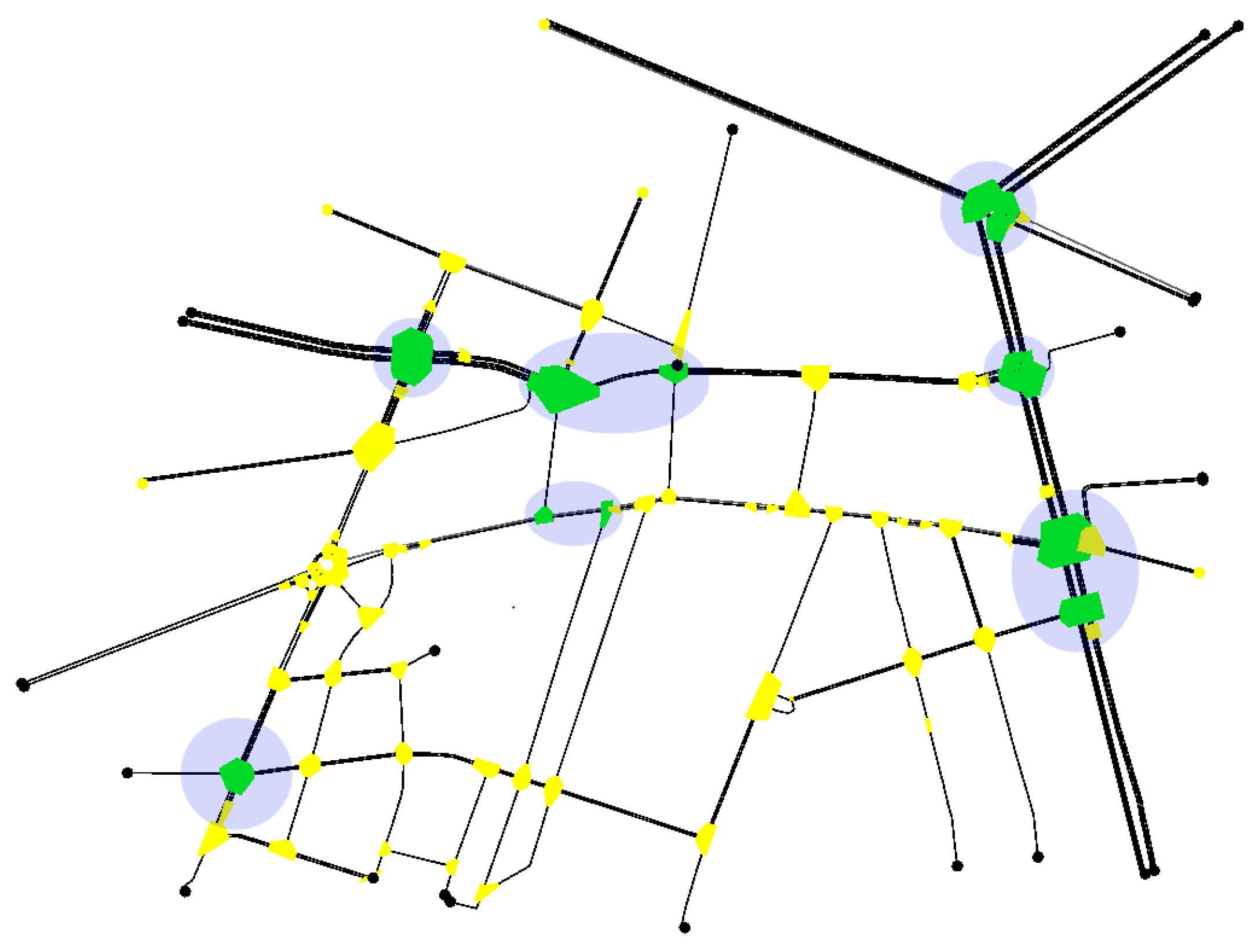
Figure 1 shows a typical experiment setting: a traffic network including multiple signalized intersections controlled by corresponding agents. Every intersection contains one or more crossroads, each including a number of lanes.
2.1. System Overview
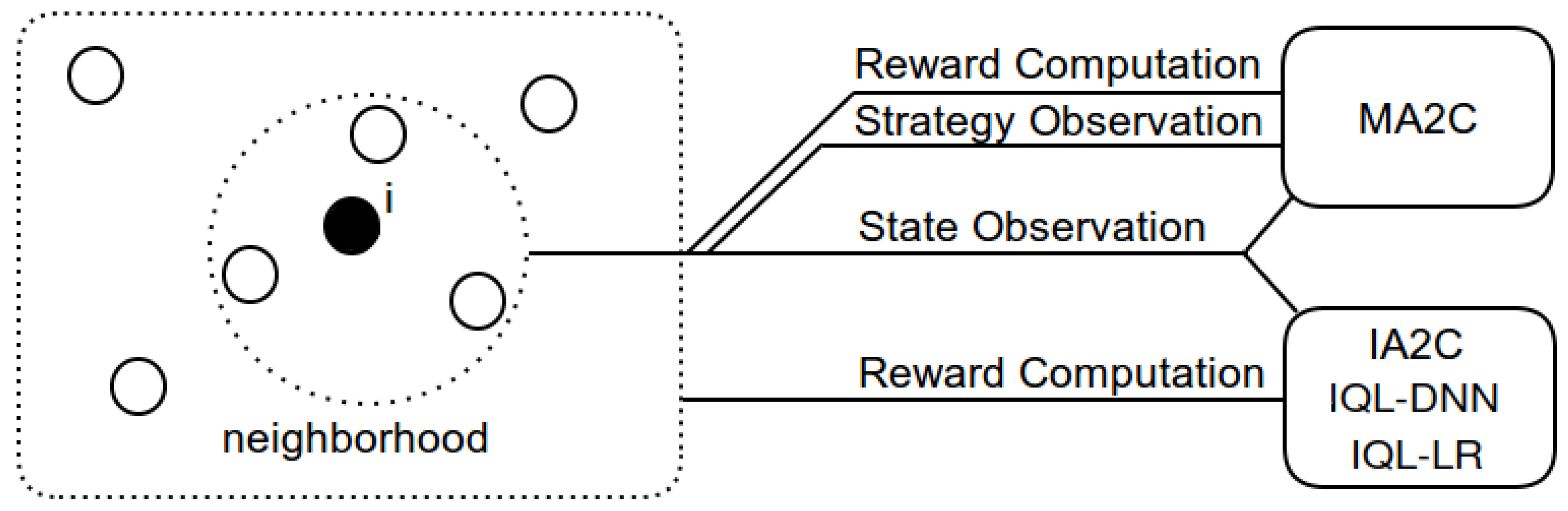
All the methods considered in this work (IQL-DNN, IQL-LR, IA2C, and MA2C) employ agents which observe the nearby vehicle flow
3 and return an action vector. The returned actions determine traffic light switching. In MA2C agents also observe the behavior of their neighboring agents, i.e. the strategy of agents located in nearby intersections. Agents trained with MA2C receive more information than the agents trained with other methods. In all cases they operate on the basis of partial information (they are not able to observe the entire state of the environment).
Another peculiarity of MA2C lies in the way the reward is calculated. In IQL-DNN, IQL-LR and IA2C, the DP reward is averaged over the whole traffic network; in MA2C, instead, the reward takes into account local traffic, i.e. the traffic in the vicinity of each agent and its neighbors. The two methods each have advantages and disadvantages. Using a measure of the overall traffic forces the agents to cooperate, but drives the learning process of each agent with a measure that is only weakly correlated to the agent’s actions. Adopting a measure of the local traffic, on the other hand, does not guarantee cooperation, but rewards each agent based on a measure that more directly depends on its actions. The latter method can promote competition between distant agents, yielding convergence towards better strategies in each group of agents. These differences among IQL-DNN, IQL-LR, IA2C and MA2C also impact the stability of the learning dynamics, as highlighted in tests.
2.2. System Formalization
From an agent’s standpoint, the problem of coordinating signalized intersections can be formalized as it follows: every
agent (i.e. every signalized intersection) aims to minimize the amount of queuing vehicles (
reward 4 ) by observing their motion in its neighborhood (i.e. by observing its neighborhood
state) and ultimately learns how to balance its
actions (control of traffic light switching) with the other agents. The IA2C agent type observes its neighborhood and, seeking its best possible strategy (
policy 5 ), encodes in its reward computation the vehicle queuing at traffic lights in the whole traffic network (
environment). On the other hand, the MA2C agent type restricts the environment reward to its neighbourhood (
Figure 2) and embeds the observation of its neighbors’ policy (
fingerprints) in its state.
2.2.1. Multi-Agent Formalization
Formally, a network of agents can be represented by a graph , where (vertices) is the set of the agents and (edges) is the set of their connections. Agent i and agent j are considered neighbors if the number of edge crossings needed to move from i to j is less than or equal to a chosen threshold. In the adopted formalism, the neighborhood of agent i is denoted and its local region is = . The distance between any two agents is denoted as with and for any .
The following list summarizes how the above introduced entities are defined in this setting:
Agent: signalized intersection
Environment: traffic network
-
Reward:
The one-step reward for agent
i at time
t cumulates the queues (number of vehicles with speed less than 0.1 m/s) at the lanes corresponding to a certain signalized intersection in the interval
:
where
is the set of lanes converging at a signalized intersection (agent)
i. The one-step reward is accrued over multiple steps to form the Reward perceived by agent
i (this step is different in MA2C, with respect to the other algorithms, as detailed in the following sections).
-
State (IA2C, IQL-DNN and IQL-LR):
The state of the IA2C, IQL-DNN and IQL-LR agents at time
t,
, is computed by:
where
[veh] measures the total number of vehicles in the set of incoming lanes (
) at time
t, within 50m from a signalized intersection (agent
i).
Action: is the action of agent i at time t (traffic light setting)
-
Policy:
agent i’s policy at time t, , is a the probability distribution over its available actions
-
Fingerprints:
policy vector set of agent i’s neighbor agents ()
State (MA2C):
where
is a multiplication factor limiting the observation of neighbor agents (
) and
is the state as defined in eq. (
2).
In this work, the states of all the considered agents will simply be referred to as when the context prevents confusion.
2.3. Background
In [
13], all algorithms were formulated under the assumption of a Markov environment. As outlined in
Section 2.2.1, the observation for each agent depends on a subset of the entire state space. To expound further, in IA2C, IQL-DNN, and IQL-LR, the observation is confined to the vehicle dynamics proximal to each individual agent. In contrast, in MA2C, each agent possesses an additional capability to observe both the vehicle dynamics and the strategy employed by its neighboring agents, providing a broader perspective, albeit still incomplete. The system should be framed in the framework of Partially Observable Decision Process (POMDP). A common way to allow the agent to observe its past states is by adopting a Long Short-Term Memory Network [
23] as detailed in
Section 2.6.1.
MA2C and IA2C rely on the history of past state observations stored in an LSTM network. In this framework the goal of the algorithm is to learn limited-memory stochastic policies
, i.e. policies that map sufficient statistics of a sequence of states
to probability distributions on actions. For IQL-DNN and IQL-LR, refer to [
13] for a fully detailed description of the algorithms.
2.4. Markov Decision Process
Reinforcement learning (RL) can be used to find optimal solutions for many problems. A Markov decision process (MDP) constitutes an adequate framework for Markovian approaches such as IQL-DNN and IQL-LR. An MDP can then be defined as a tuple with its contents defined as follows:
is a set of states, where denotes the agent’s state at time t.
is a set of available actions, where denotes the action the agent performs at time t.
is a transition function and denotes the probability of arriving at state when action is performed in state .
is a reward function where is the reward when the agent transitions from state to state after performing action .
is a discount factor.
The transition function p is often referred as the model of the system as it captures its dynamics. All the algorithms considered in this work are model free, i.e. every action yields a state change with probability 1, and all other transitions have probability 0. In general may depend on but in the studied case (signalized intersections) doesn’t depend on .
2.4.1. Single Agent Recurrent Policy Gradients
For IA2C and MA2C, which rely on partial observability and are equipped with a memory as discussed in
Section 2.3, the MDP described in
Section 2.4 is not an adequate description. In this case the environment still produces a state
at every time step but state transitions are governed by a machinery dependent upon its previous actions
and the previous states
of the system.
In this more general setting, the agent has a memory of its experience consisting of finite episodes. Such episodes are generated by the agent’s behaviour in the environment: in each time step t, the agent observes , performs action , and receives a reward whose expectation depends solely on and . We define the observed history as the sequence of states and actions from the beginning of the episode up to time t: .
With an optimal or near-optimal policy for a POMDP, the action is taken depending on the preceding history.
Let
be a measure of the total reward accrued during a sequence of states, and let
be the probability of a state sequence given policy-defining weights
. An optimal policy will minimize
This, in essence, indicates the expected reward over all possible (selectively remembered) sequences, weighted by their probabilities. Using gradient descent to update parameters
:
using the likelihood-ratio "trick" [
24] and the fact that
as the accrued reward
does not depend on
. Accordingly, the loss gradient can be rewritten as:
where
is the only term depending on
.
In the above computations, the whole state-action sequence is denoted with
. The entire sequence is unnecessary, and the agent only needs to learn sufficient statistics (referred to as
history hereafter)
of the events, representing the limited memory of the agents’ past. Thus, a stochastic policy
and history
can be redefined by the position
6, and implemented as a Long Short-Term Memory (LSTM) network with weights
. This produces a probability distribution
, from which actions are drawn. Accordingly,
can be further subdivided:
As in the Markov policy gradient case, all the p terms will be split into a sum of logarithms and be removed, since they do not depend on .
Performing Monte Carlo sampling for the whole episode length, the loss
can be approximated as in the following formula:
where
is the number of sampled episodes and
is the number of time steps in an episode.
Introducing batch learning and iterating over sampled episodes, the training procedure aims to minimize the following loss.
where the episode index has been omitted.
In equation (
9),
is the number of time steps in the batch;
is the aggregated reward over the batch, given by
, where the usual
discount factor has been introduced [
6];
is sampled from
.
2.4.2. Single Agent Recurrent Advantage Actor Critic
In accordance with the formulation in
Section 2.4.1, the derivation of the loss functions for Recurrent Advantage Actor-Critic (A2C) in the context of a POMDP is undertaken. The Actor’s loss is:
while the Critic’s loss is:
where:
and are the histories of past events registered by the two LSTM networks used to compute the regressors and
is the
n-step return [
6], with
; the regressor for state value at
(corresponding to the first time step of the next batch) is evaluated using the current parameters
is the sampled advantage for actions
In the above definitions,
is the set of the Critic’s parameters computed at the last learning step (current Critic’s parameters); accordingly, in the next sections
will denote the set of the Actor’s parameters computed at the last learning step (current Actor’s parameters)
7. Notably, the inner states of the Critic’s LSTM are not updated when computing
as
corresponds to the first time step of the next batch. This prevents the state sequence (history) from being compromised when the state value is computed while processing the next batch.
2.5. Multi-Agent Policy-Gradient Systems
2.5.1. Independent Advantage Actor-Critic (IA2C)
In IA2C, each agent i learns its own policy and value function collecting experiences from its own DP. The observation of agent i is restricted to , i. e. .
The loss functions for the Actor and Critic are:
where:
with
In the above, and are the Actor and Critic’s network parameters, and a ’-’ superscript indicates their current values; as a parameter subscript refers all the agents except agent i.
When training begins, all actions have similar probability. To encourage exploration, the entropy loss of policy
has been added in (
12), weighted by the parameter
.
Restricting the observation of agent i to affects both and via . On the one hand, this yields partial observability while on the other hand, since is dependent on the whole , it allows and to converge towards optimum values specific to agent i. This is especially important for as, without a restriction on the agent’s observation, all the agents will seek the same global optimum , while every has its own specification in terms of type and number of available actions.
2.5.2. Multi-Agent Advantage Actor-Critic (MA2C)
MA2C [
13] improves the stability of the learning process by allowing some communication among agents belonging to the same neighborhood; a spatial discount factor weakens the reward signals from agents other agents than
i in the loss function, and agents not in
are not considered in the reward computation. Equations (
12) and (
13) become:
In the above equations:
-
with
The spatial discount factor
penalizes other agent’s rewards
8, and
is the limit of agent
i’s neighborhood.
Equation (
15) yields a more stable learning process since (a) fingerprints
are input to
to bring in account
, and (b) spatially discounted return
is more correlated to local region observations
By inspection of equations (
12,
13,
14,
15), the peculiarities of MA2C with respect of IA2C can be summarized as: 1) MA2C uses fingerprints, 2) MA2C uses a spatial discount factor, 3) the overall reward (
in MA2C) is computed on
instead of the whole set of agents
.
2.6. System Architecture
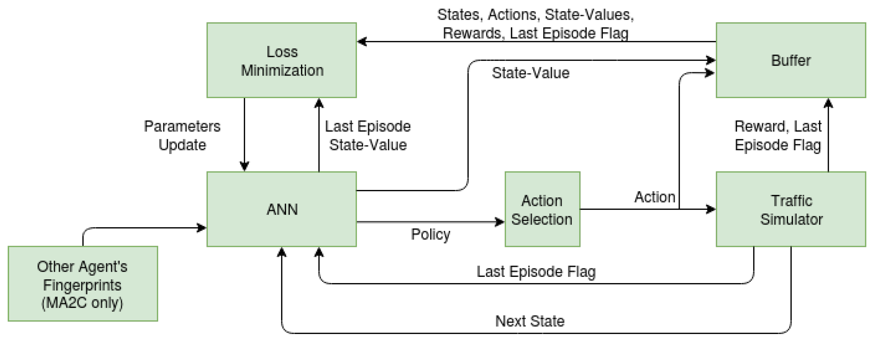
Figure 3 provides an overview of the system.
As stated in the previous sections, the goal is to minimize the vehicle queues measured at signalized intersections. To this end, the following steps are repeated: 1) An ANN takes as an input the perceived state of the environment and provides a policy. For MA2C, the environment state includes the policies of its neighbor agents (fingerprints). 2) An action is sampled from the provided policy and passed to the traffic simulator, which performs a simulation step and returns the new environment state and last episode flag (a flag indicating whether the episode is over) to the ANN. The simulator also stores actions, rewards, and the last episode flag in a buffer. These two steps are repeated until the buffer (here denoted batch) is full. 3) the ANN uses the stored rewards to change its parameters and improve its policy.
2.6.1. ANN Detail
For IQL-DNN and IQL-LR, see to the multi-perceptron ANN details in [
13]. For MA2C and IA2C, states, actions, next states and rewards are collected in batches called experience buffers, one for each agent
i:
. Batches are stored while the traffic simulator performs a sequence of actions. Each batch
i reflects agent
i’s experience trajectory.
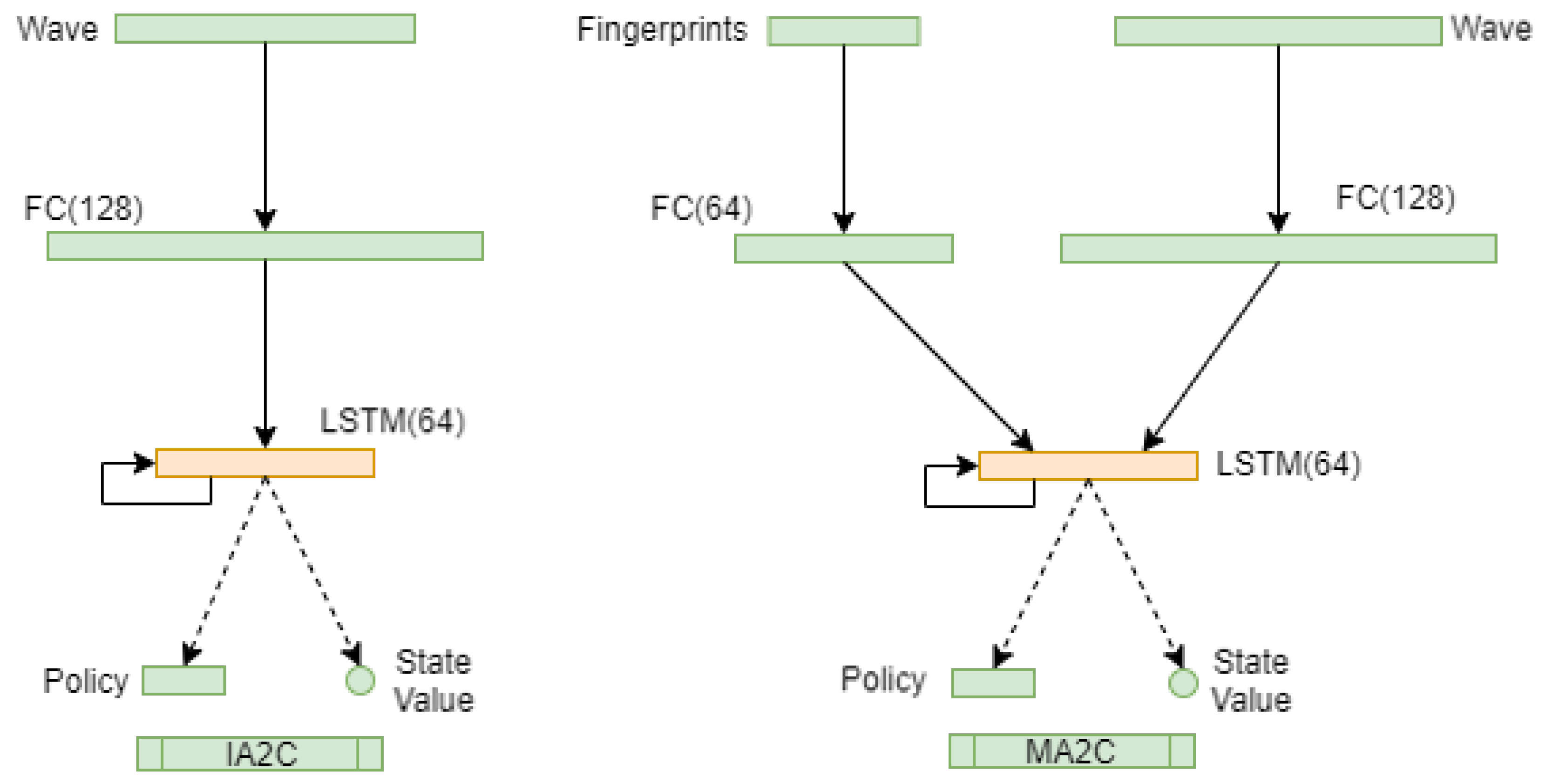
Figure 4 shows the IA2C and MA2C architectures.
This architecture is used for each agent so 2 ANN’s are instantiated. In IA2C (left), the first layer is formed by a variable number of input neurons that encode wave measures, i.e. the total number of approaching vehicles along each incoming lane, within 50m. The second layer is formed by 128 neurons. The third layer is formed by 64 LSTM units. The first layer is fully connected to the second layer. The third layer is fully connected to itself and to the fourth layer.
In the case of the MA2C method (
Figure 4., right), the first layer is formed by a variable number of input neurons encoding wave measures and by a variable number of neurons encoding the action vectors of nearby agents. The second layer is formed by two groups of 128 and 64 neurons that receive connections from the two groups of sensory neurons described above. The third layer is formed by 64 LSTM units. The first layer is fully connected to the second layer; the third layer is fully connected to itself and to the fourth layer.
The network architecture reflects the A2C formalism [
25]; each graph represents two different networks, one for the Actor (policy) and one for the Critic (state value), with their respective parameters here denoted as
and
. The fourth layer of the Actor network is formed by N neurons with a softmax activation function, which encode the probabilities of choosing one of the N corresponding possible red-green-yellow transitions of the corresponding traffic light. The fourth layer of the Critic network is a single neuron that encodes the expected reward. The neurons of the second and third layer use the rectified linear unit (ReLU) activation function. For ANN training, an orthogonal initializer [43] and an RMSprop
9 gradient optimizer have been used. To prevent gradient explosion, all normalized states are clipped to [0, 2] and each gradient is capped at 40. Rewards are clipped to [-2, 2].
3. Calculation
We evaluate MA2C, IA2C, IQL-DNN and IQL-LR in SUMO-simulated traffic environments replicating two districts in the Bologna area (Andrea Costa and Pasubio) [
26]. While these traffic networks are similar in the required number of agents, they differ significantly in their topology, allowing evaluation of how topology influences the learning process. Every episode of the SUMO simulation consists of 3600 time steps. For a pre-determined interval of time, a vehicle is inserted in the traffic network at each time step a with a random origin-destination (OD) pair.
To ensure a fair evaluation of the algorithms, identical settings for experimental parameters (except those parameters specific to each algorithm [
13]) have been adopted. The criterion used to evaluate the algorithms’ performance is the queue at the intersections, which is linked to the DP reward by equation (
1). Queues are estimated within SUMO for each crossing and then passed as rewards. In testing, the algorithms have been compared with a greedy approach (hereafter denoted Greedy) which simply selects the traffic light phase associated with the largest
over all incoming lanes. For the pseudo-random experiments reported in the following sections, the seed is kept constant during collecting training samples, while different seeds are used in the 8 testing episodes
10. For the fully stochastic experiment (reported in
Section 4), the seeds are kept constant only during each episode; when testing, seeds are changed for each of the 8 episodes, like in the pseudo-random case. For brevity, “veh" is a shorthand for “vehicles”.
The DP is instantiated with the settings listed in
Table 1.
The size of the batch indirectly sets the
n parameter of the
n-step return appearing in Equations (
12), (
13), (
14), and (
15) and has been chosen to balancing the complementary characteristics of TD and Monte-Carlo methods [
6]. With a forward step limit at 1000800 and the settings reported in
Table 1 for
,
t and
, a complete learning process results in 278 episodes (i.e. 5004 learning steps).
3.1. Algorithms
The presented tests do not rely on a structured configuration of the vehicles in motion
11. In fact, assuming a traffic macro-behavior in terms of general vehicle flows is beneficial when the flows effectively reflect the real traffic macro-behavior; but this is seldom the case in practice and such assumptions might instead cause overfitting [
27] originating from spurious regularities. To avoid this issue, pseudo-random Origin Destinations (OD) pairs are assigned to each vehicle. This allows the learning process to achieve a more general optimum as the equilibrium among the agents doesn’t depend on any specific assumption on the flows or boundary condition. Our experimentation consists of the following steps:
Loading traffic networks with a varying number of vehicles.
Evaluating the training graphs of IQL-DNN and IQL-LR.
Comparing the IA2C and MA2C learning curves
Comparing MA2C with IA2C and Greedy
Evaluating the behavior of the learning curves for IA2C and MA2C
Evaluating the effects of the learned policies in terms of traffic volumes
3.2. Traffic Networks
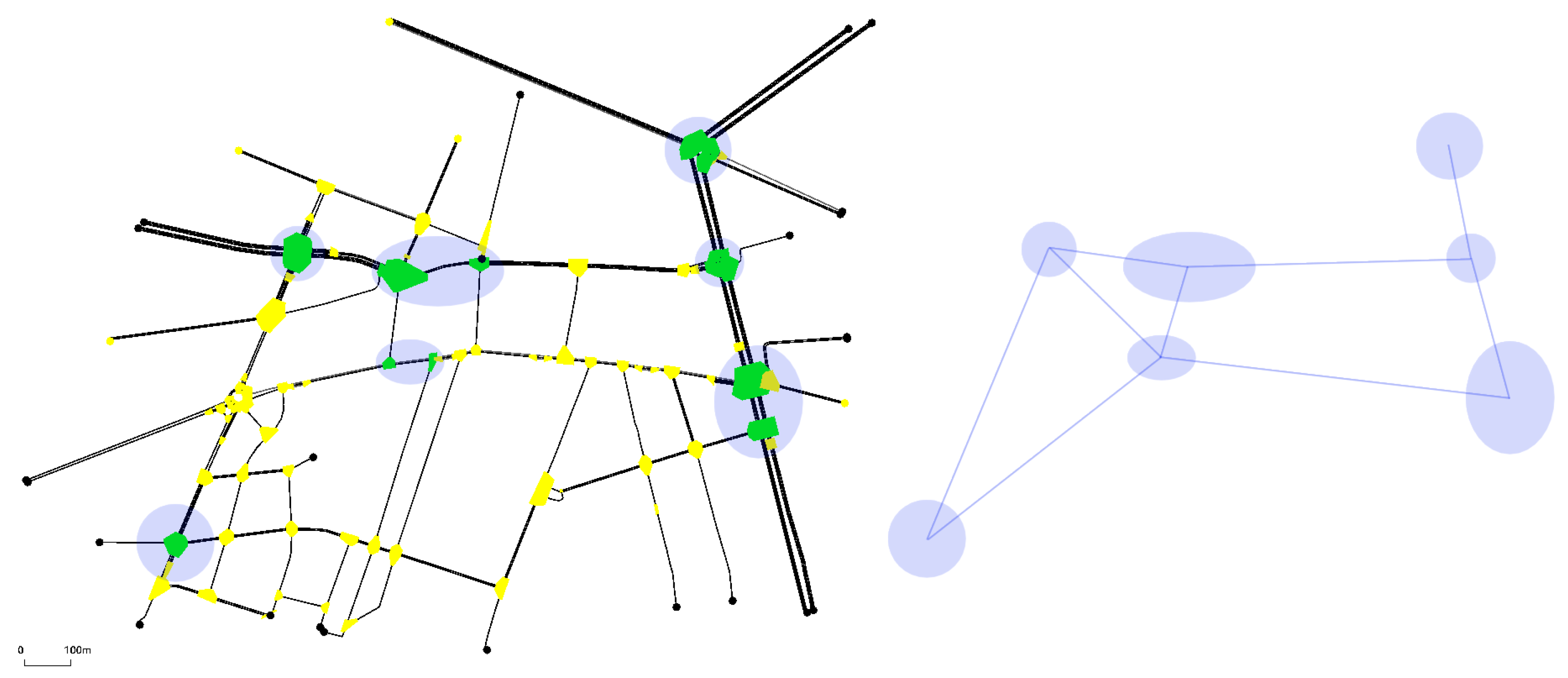
Figure 5 (left) shows the Andrea Costa neighborhood of Bologna [
26].
The round/elliptic (purple) shaded spots identify the signalized intersections (agents). The right side of the figure shows the way each agent is connected to the others. The set of all the agents connected to a single agent constitutes its neighborhood.
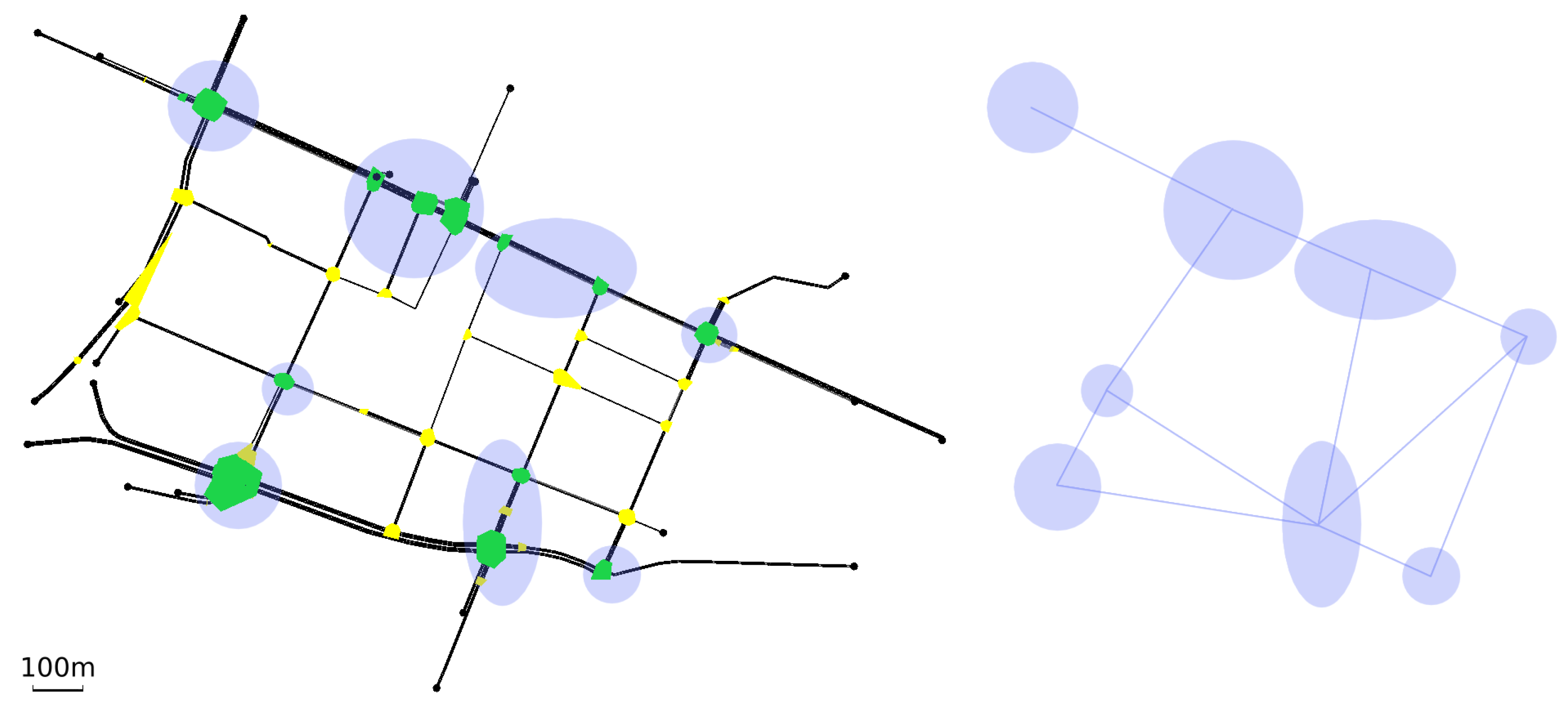
Figure 6 (left) shows the Pasubio neighborhood of Bologna [
26]. As in the Andrea Costa case, the right hand side of the figure shows how the agents have been connected.
The vehicle insertion procedure over each episode of 3600 time steps is divided into the following alternatives:
One vehicle inserted per time step for the first 2000 time steps, then no more vehicles for the remaining time steps, totalling 2000 vehicles
One vehicle inserted per time step for all 3600 time steps, totalling 3600 vehicles
Two vehicles inserted per time step for the first 2000 time steps, then no more vehicles for the remaining time steps, totalling 4000 vehicles
3.3. IQL-DNN and IQL-LR
In agreement with the results reported in [
13]
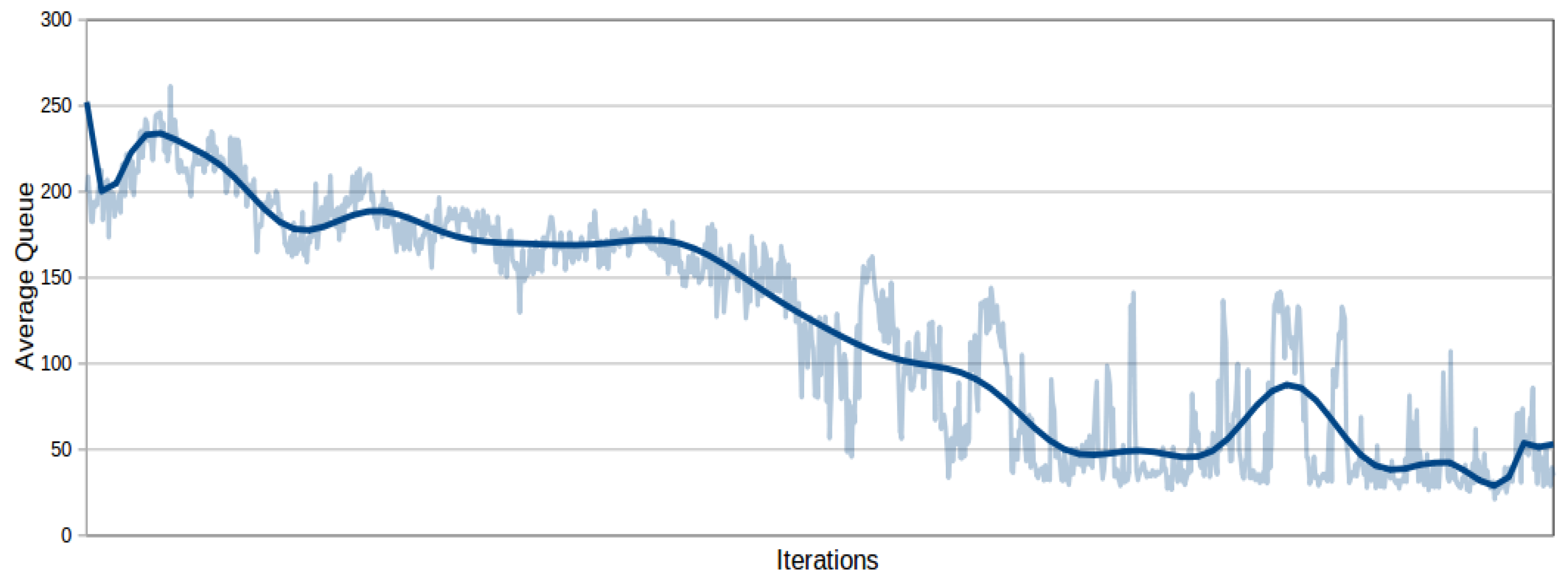
12, IQL-DNN and IQL-LR algorithms perform rather poorly in the traffic networks, even in the simplest case (2000 vehicles).
Figure 7 and
Figure 8 show the performance of the two algorithms in terms of the overall average queue
13. The graphs show that the algorithms have a divergent trend and then stabilize around 500.000 interactions to a value significantly worse than the original setting
14. In view of this result IQL-DNN and IQL-LR have been excluded from further experimentation with real traffic networks, as was done in [
13]
15
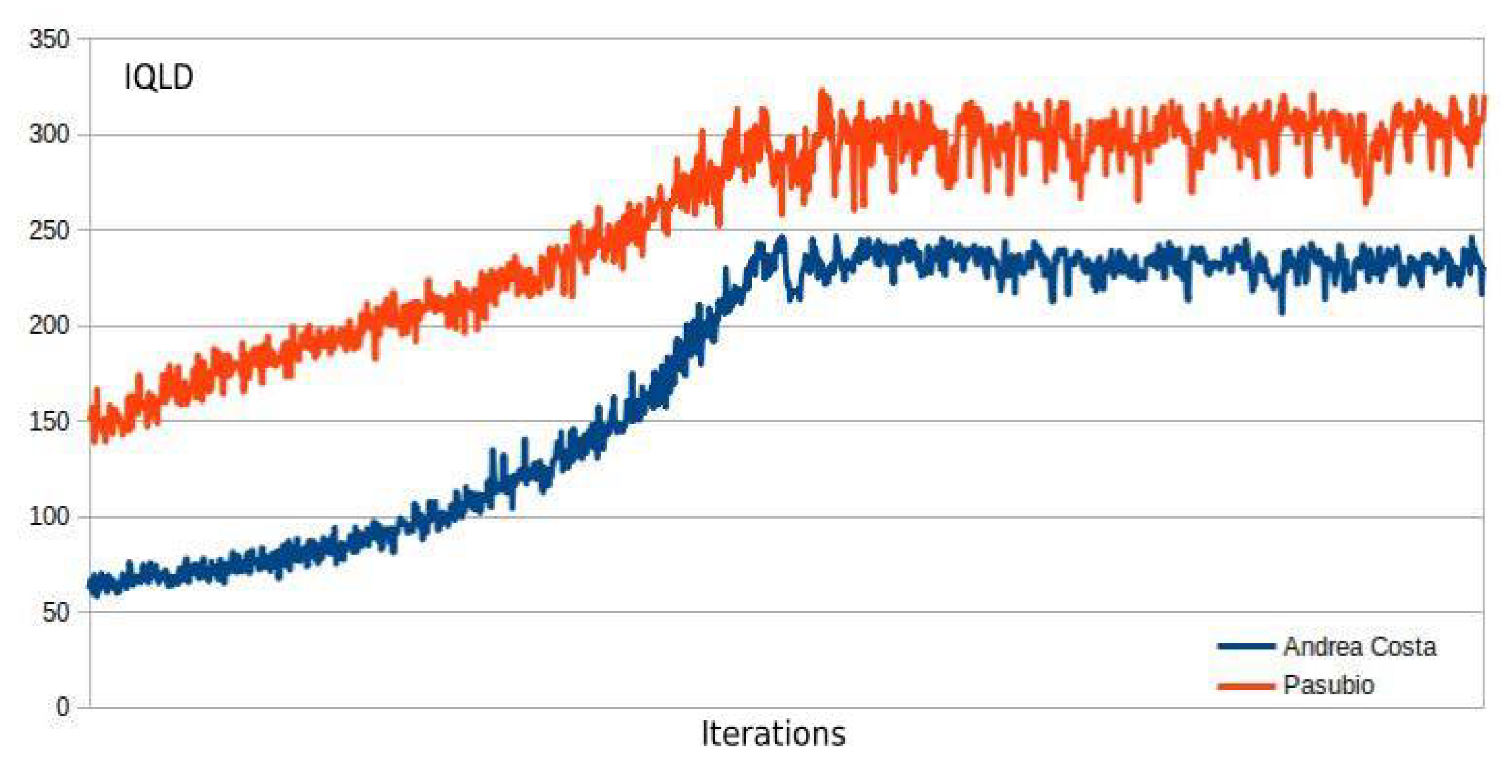
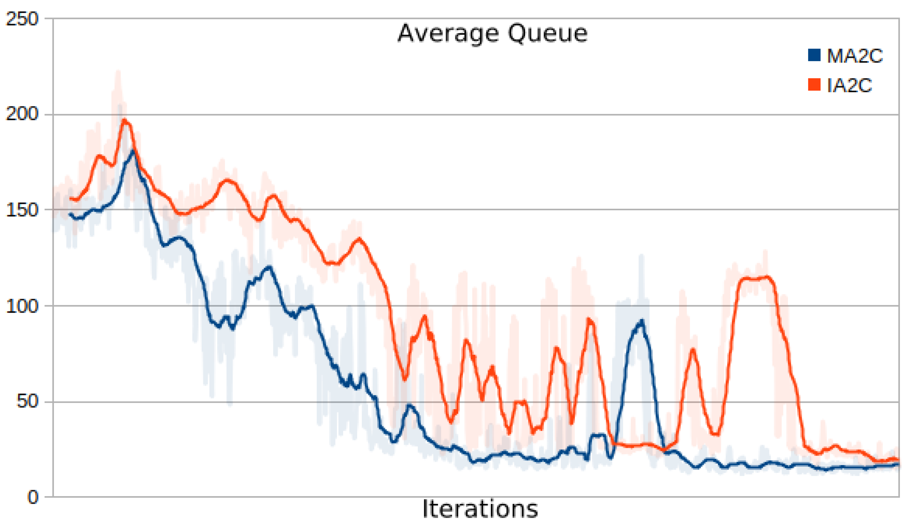
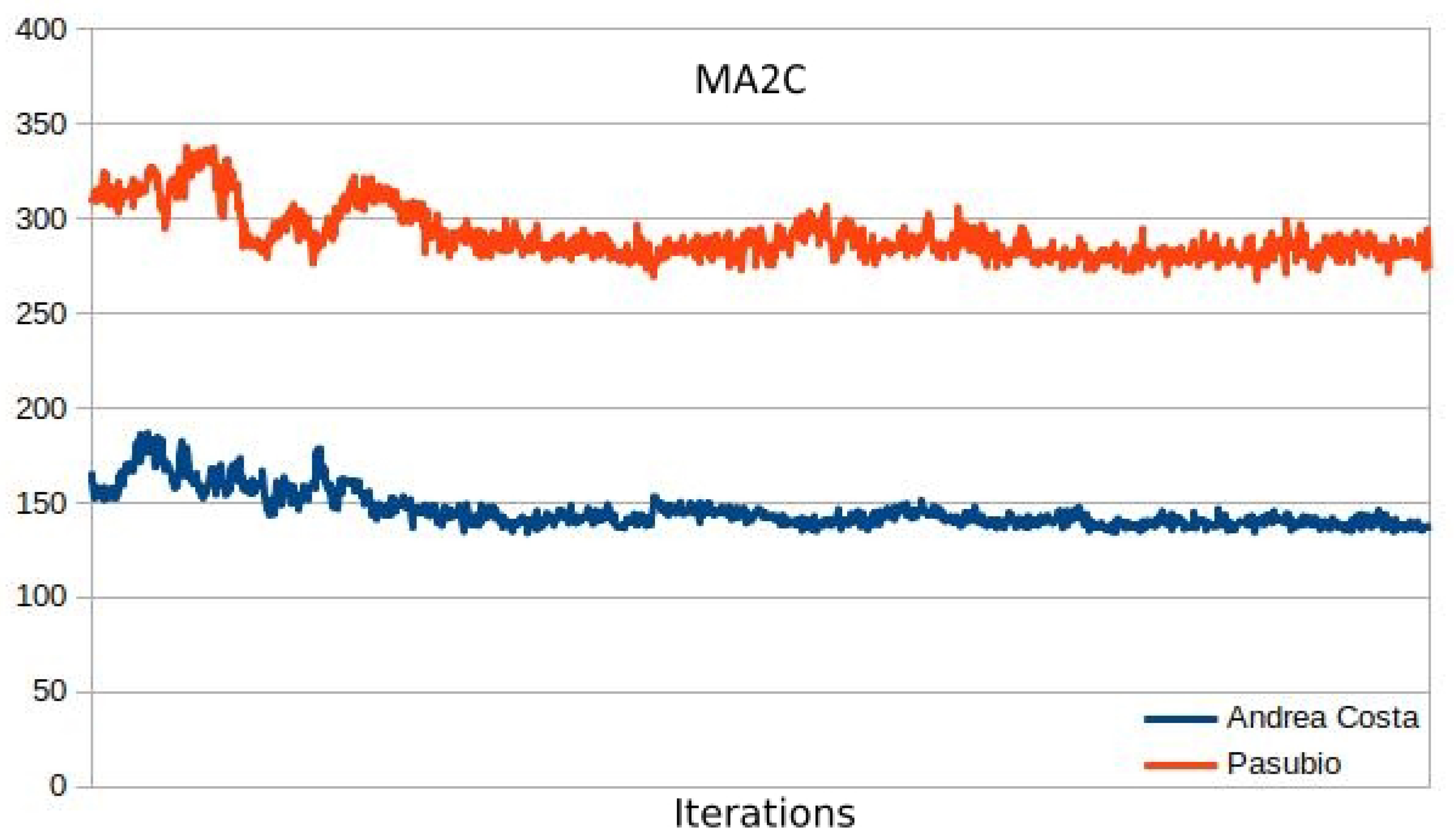
3.4. MA2C and IA2C Performance on the A. Costa Traffic Network
Figure 9 and
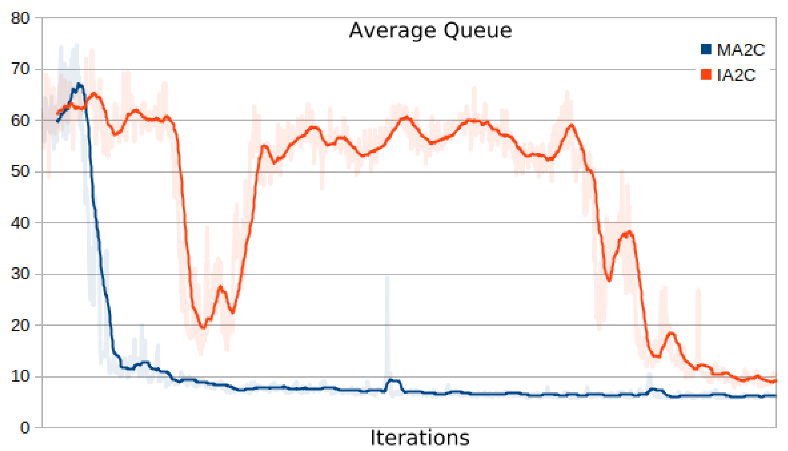
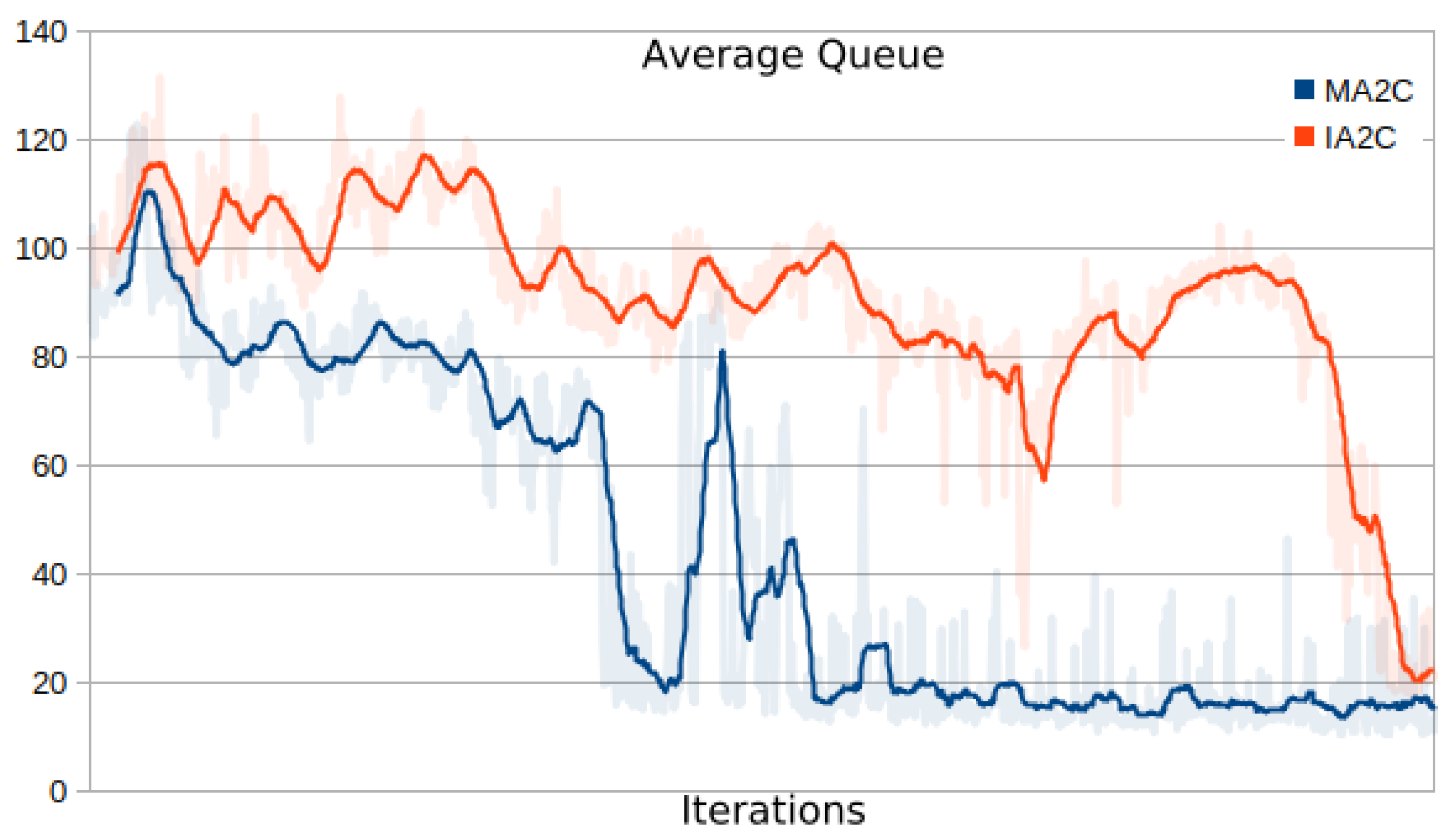
Figure 10 show the minimization of the average queue on the traffic network loaded with 2000 and 3600 vehicles. While both the MA2C and IA2C learning processes achieve a similar minimum, the curves appear very different: while MA2C achieves a stable point from iteration
onward, IA2C is much less steady. Particularly in
Figure 10 (load of 3600 vehicles), IA2C achieves its optimum (which, as shown in Figure 15 is the only success out of 10 learning runs) only in the very end of the process.
Table 2 and
Table 3 show the average queue length for 8 tests, with different random seeds for each test. The average and standard deviation across these tests are also shown. MA2C appears better than IA2C in
Table 2, and evidently outperforms Greedy.
The average queue measured is similar to the achieved minimum in the training process, showing that even though the system was trained with pseudo-random simulations, the final result doesn’t appear to overfit on specific sets of origin-destination (OD) pairs. This is especially important because it verifies that the learning process focuses only on dynamics occurring in the vicinity of the traffic lights. RL is known to have a tendency to overfit when the training dataset is a subset of all potential cases [
27]; training with real data is challenging for this application as transforming integrated traffic flow data into OD matrices requires mixed heuristic-deductive reasoning [
29].
In the next sections, this relevant finding will be confirmed by further experimentation.
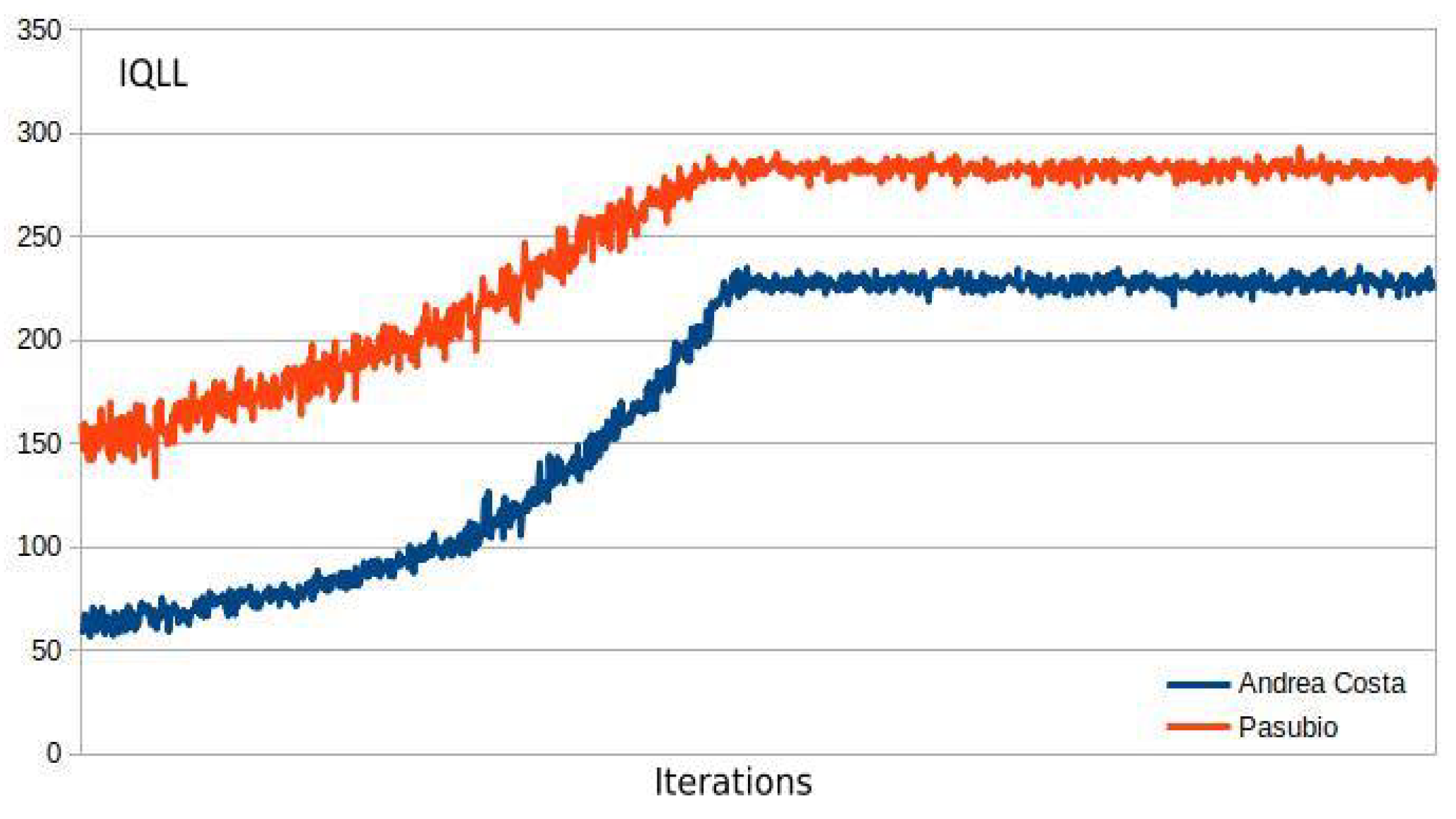
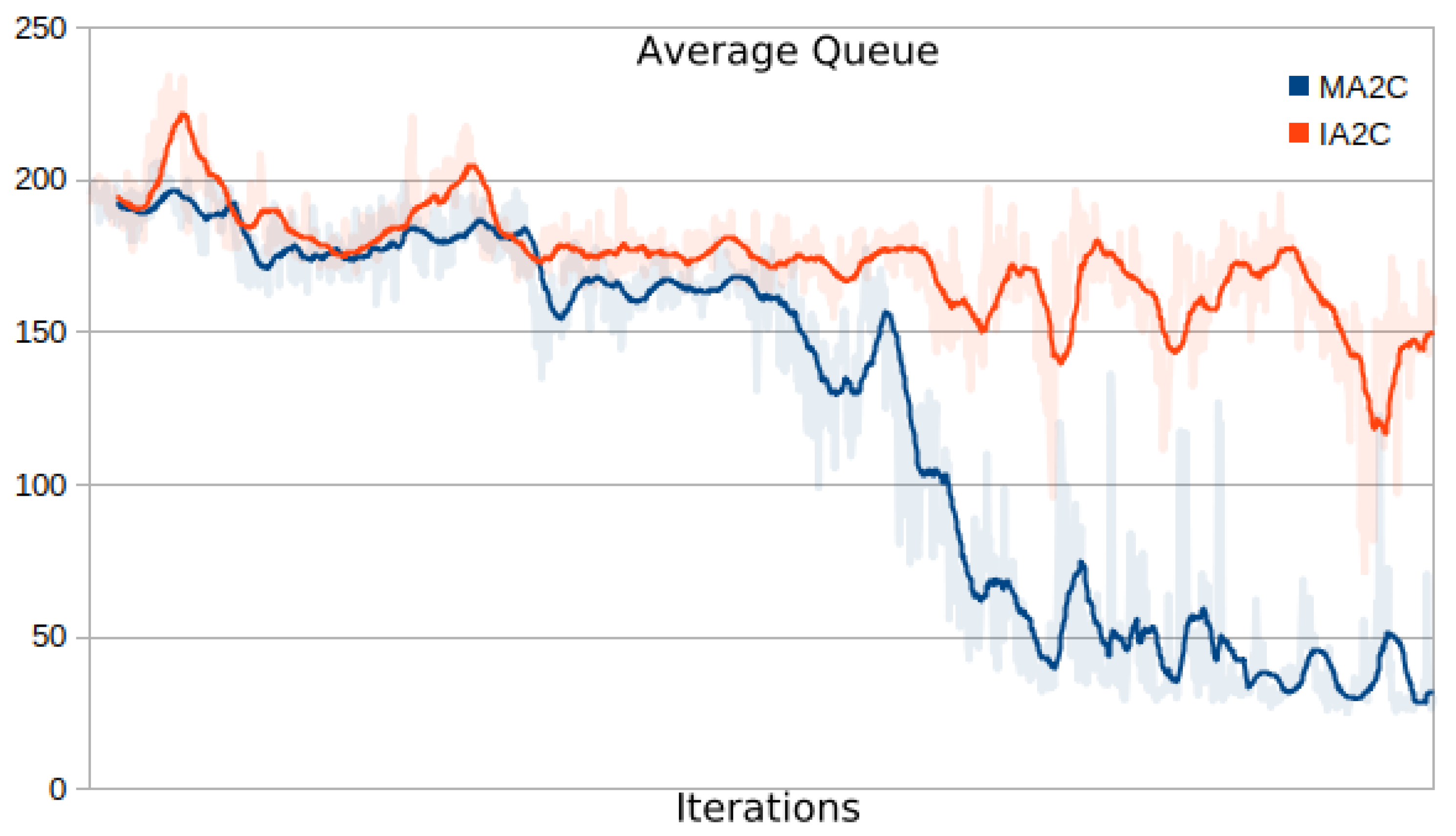
3.5. MA2C and IA2C on the Pasubio Traffic Network
Figure 11 shows the training graph for the case of 2000 vehicles circulating in the Pasubio traffic network. The figure shows that MA2C is able to achieve an improvement while IA2C showed a much more oscillatory behavior during training. As a result, when measuring performances with 8 different test seeds, the average queue measured are very different in the two cases (
Table 4 and
Table 5). Notably, in
Table 4, MA2C exhibits a slightly worse behaviour than the Greedy approach.
The case of 3600 vehicles was more challenging for MA2C and IA2C (
Figure 12). While optimization of IA2C failed across 10 learning runs, MA2C was successful in 6 runs out of 10 (Figure 15). In testing, MA2C was more effective than the Greedy policy, which showed a larger average and a much larger variance in the 8 tests.
3.6. Further Tests
To further evaluate the capabilities of MA2C in managing an increased vehicle flow, 2 vehicles per time step for the first 2000 time steps have been inserted, totalling 4000 vehicles in the traffic network. We carried out 10 training attempts, for both the Andrea Costa and Pasubio traffic networks. Across these experiments, MA2C behaved similarly. The loss increased in the initial training stage, followed by learning in the following steps, but without substantial improvement in terms of the average queue of vehicles as shown in
Figure 13.
Though this behaviour highlights MA2C’s limitations in dealing with high volumes of traffic, the next sections will show that MA2C still represents a better alternative than the other algorithms, even in this case.
4. Convergence Stability
This section is devoted to the convergence analysis of the learning process: given the IA2C and MA2C algorithms, the goal is to evaluate if there are theoretical guarantees for the loss minimization process towards a relative minimum. To this end, three issues should be considered: first, the non-Markovian nature of the decision process; second, the non-stationary aspect of the problem: besides the inherent non-stationary nature of the environment, when the agents’ policies evolve during the learning process, from the viewpoint of each agent, the environment changes, due to the changing policies of the other agents; third, each agent has access only to a subset of the overall system state, namely the state of the neighboring agents.
As depicted in
Figure 2, IA2C and MA2C differ in the computation of the DP reward, which, in turn, enters in the computation of the loss: while IA2C considers the contribution of all the agents in the traffic network, MA2C restricts its scope to each agent’s neighborhood. This makes the stochastic game determined by the IA2C agents fully cooperative, while MA2C is mixed cooperative-competitive. The input of the neural network adopted to determine value and policy is different in the two cases: both the approaches refer each agent’s neighborhood but only MA2C uses as an input the learning policies from the other agents. Presently, there is no theory general enough to encompass the complexity of IA2C and MA2C. In the following sections, the theory framework behind general Multi-Agent Reinforcement Learning (MARL) problems is surveyed, emphasizing the theoretical limits of the convergence guarantees. These limits hinder their application to IA2C and MA2C.
4.1. Theoretical Evaluation of the Learning Process
In [
30] an approach is proposed that links instances of NMDP to probabilistic-deterministic finite automata yielding regular decision processes (RDP). Following this proposed method, it is possible to define a
Markov abstraction [
30] that reduces the problem to solving an MDP instead of an RDP. In general, LSTM cells have the potential of relying on infinite histories, but in episodic RL the history length is limited by the length of episodes and can be modeled with finite automata.
Formally, a Markov abstraction over a finite set of states S is a function
such that, for every two histories
and
and every action
,
implies
, where
, the
dynamics function, describes the probability of observing a certain pair of observation and reward (or episode termination) in the next time instant, given a certain history
h and action
u. Since the dynamics are the same for every history mapped to the same state, there is an MDP
with dynamic function
(the
induced MDP) which can be solved in place of the original RDP
[
30]. It is straightforward to see that the machinery due to the presence of an LSTM cell in the ANN shows no significant difference with the Markov abstraction defined in [
30] for the case of a single-agent DP. For the multi-agent case, there is no such correspondence, as any such abstraction must account for the number of agents participating in the stochastic game and any limits on the rate of change of their policies.
Work on convergence of actor-critic decentralized MARL has been reported in [
27,
31,
32] and in [
33], which focuses on vanilla Actor-Critic. In [
31] the proposed theoretical tools extend the approach described in [
27] to the case of deterministic policies. As confirmed in [
32] and [
31] at the present [
27] represents the state of the art on theoretical studies on stability and convergence of the learning process. The non-stationarity issue is not extendable to the multi-agent case as "theoretically, if the agent ignores this issue and optimizes its own policy assuming a stationary environment [...] the algorithms may fail to converge, except for several special settings. Empirically independent learning may achieve satisfiable performance in practice" ([
34]). in [
27] there are theoretical tools able to determine that the policy parameter
(referring agent agent
i) obtained from the presented A2C algorithm converges almost surely to a point in the set of asymptotically stable equilibria. Besides the above mentioned non-stationarity issue, in [
27] there are limitations preventing the theory to be applied to the IA2C and MA2C cases. The most stringent limitations regard the state observation that in [
27] is complete, while in both IA2C and MA2C is partial
16, and the adoption of linear function approximation while IA2C and MA2C rely on non-linear ANNs.
To summarize, a theory able to formally provide convergence guarantees for the learning process in IA2C and MA2C is still lacking, due to difficulties in extending the link between NMDP and MDP to MARLs and some simplificative hypotheses when formally dealing with non-stationarity and observation (see [
27] for details) that cannot be applied to IA2C and MA2C.
4.2. Experimental Evaluation of the Learning Process
Some heuristic analysis of the learning process is possible by inspecting the average queue curve during learning.
A tendency to diverge from asymptotic behaviour, oscillations, or spikes show that the agents have not found a steady balance: even when a solution is found, queues at each signalized intersection can both shrink and grow during a single episode. As discussed in the previous section, when ANNs are coupled with Reinforcement Learning, a challenging task arises from pursuing a changing target during the learning process. In the multi-agent case, targets are even more elusive: an agent, e.g. agent i, converges smoothly towards an optimal policy as long as stay constant. This is not the case in a collective learning process where other agents’ changing policies affect their behaviour. This in turn affects (from the decentralized view point) the expected return of agent i. Eventually, this sequence of causal relationships can make the learning process inconsistent. This issue can happen even if agent i finds an ideal policy: changes of might cause the agent i to slip away from its optimum. Ideally, all the agents find their optima at roughly the same time.
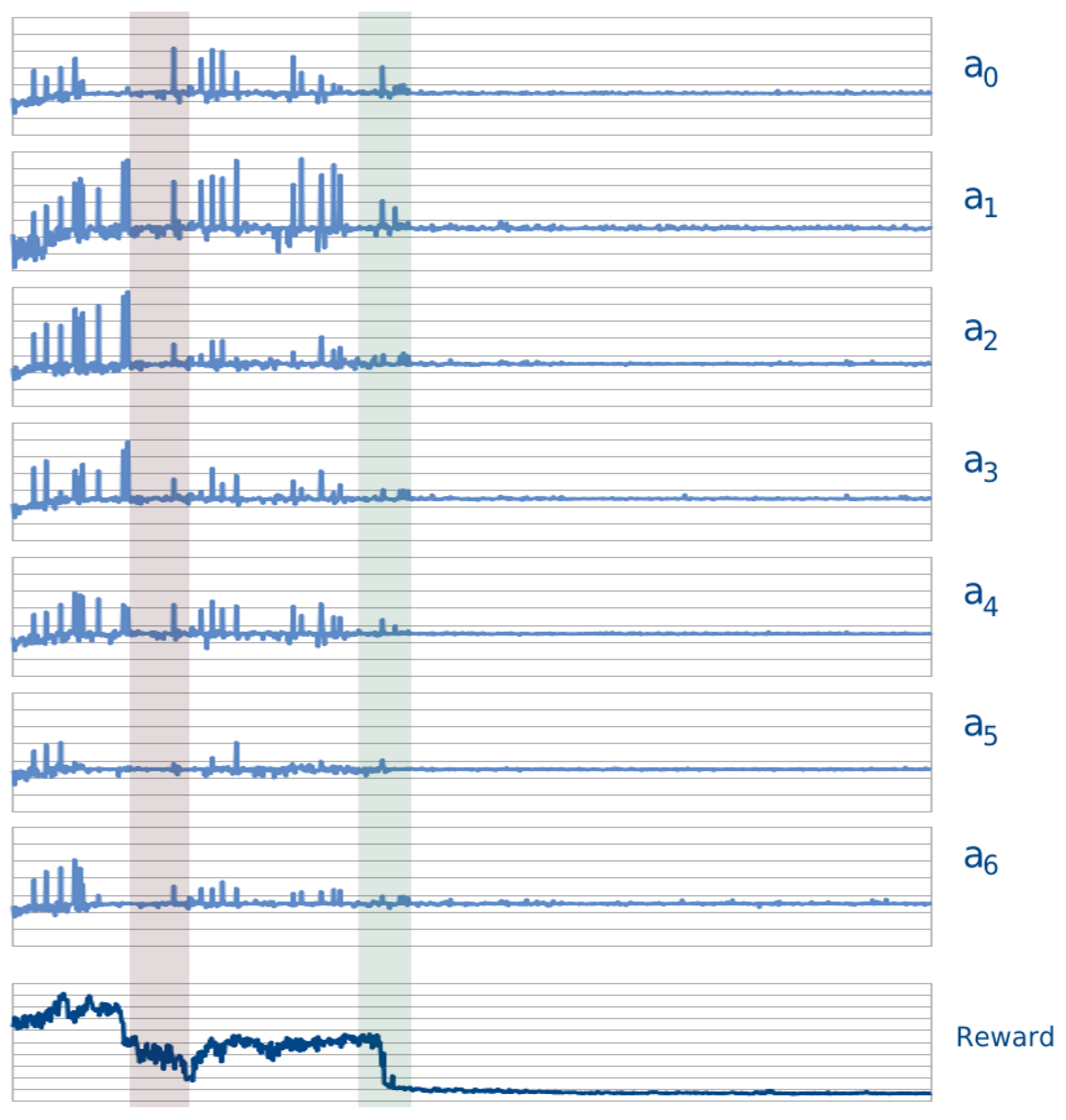
As an example of this problem,
Figure 14 shows the behaviour of the seven agents in the Andrea Costa case, when loaded with 2000 vehicles as described in Sec.
Section 3.2. The top graphs show the behaviour in time of the Actor’s loss for agents
during the learning process. The bottom graph shows the reward, as the averaged cumulative queues evolve in time. The left (red) shaded region highlights the inconsistency issue: at the beginning of the shaded region agent
is slightly unstable (while the other agents appear to be close to a relative balance) and eventually drags away the other agents from their converging path. In the (green) shaded region on the right, instead, all the agents appear to move together to a common relative minimum; this is especially evident observing agents 0, 1 and 4.
To limit the occurrence of such inconsistencies it is beneficial to maintain the learning process as smooth as possible; this is achieved by keeping small
17 by updating the target of the optimization process after each learning step.
The overall consistency of the algorithms during training can be evaluated by observing that the properties of the environment change significantly depending on quantitative factors. For this reason, the results obtained with IA2C and MA2C are compared in three experimental settings with varying number of vehicles introduced in the traffic networks:
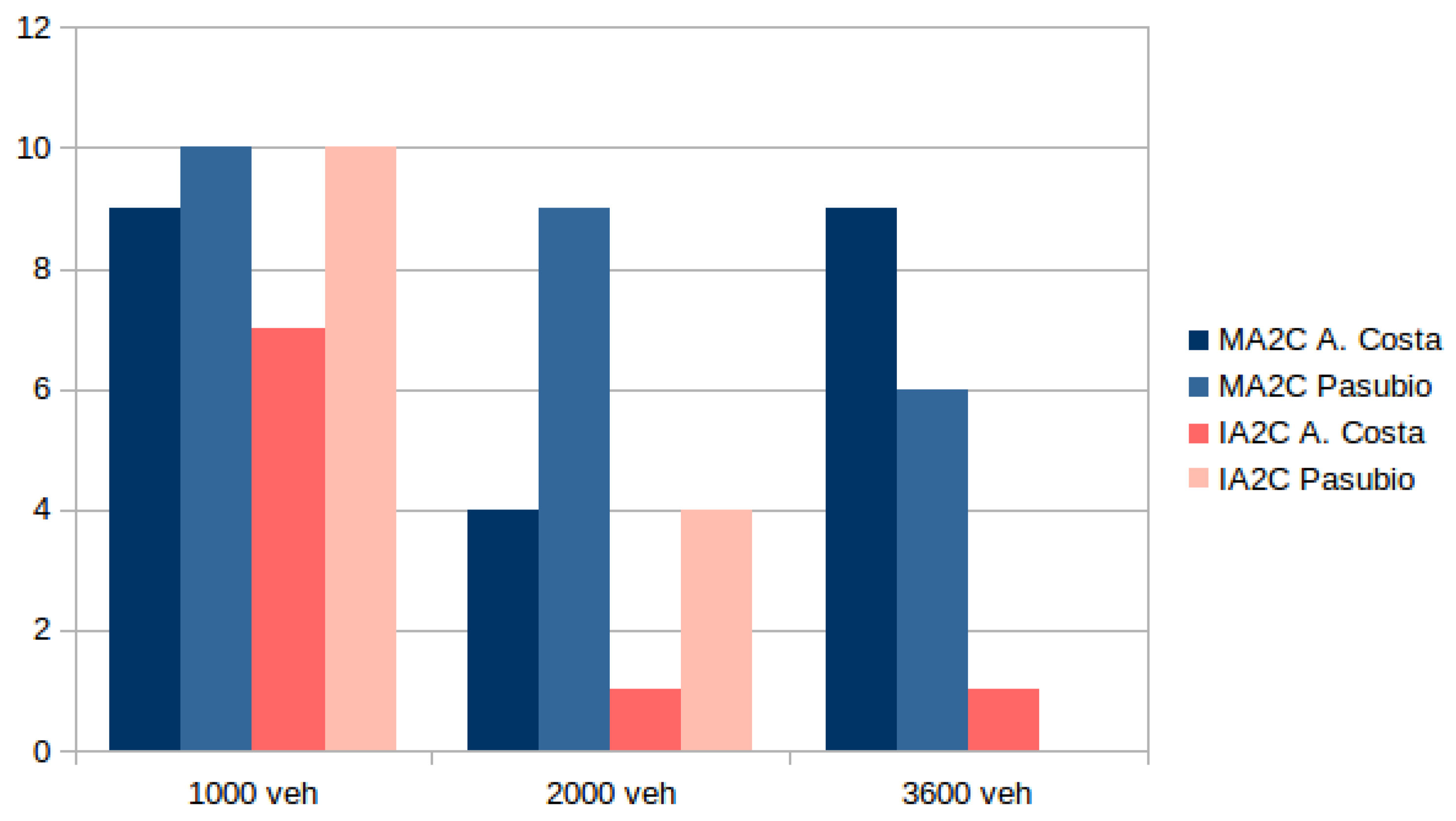
Figure 15 shows the number of training successes across 10 learning attempts for the cases with 1000, 2000 and 3600 vehicles in both the A. Costa and Pasubio networks.
As evident in
Figure 15, MA2C is more stable than IA2C. The learning processes tend to become more inconsistent when the vehicle load increases, with the notable exception of the A. Costa case loaded with 2000 vehicles, which shows much more problematic than the case with 3600 veh. It is interesting to observe that, while this case is more unsteady than the 3600 case, the graph of the A. Costa case loaded with 2000 vehicles displays a much less oscillatory behaviour once convergence is achieved, as highlighted in the
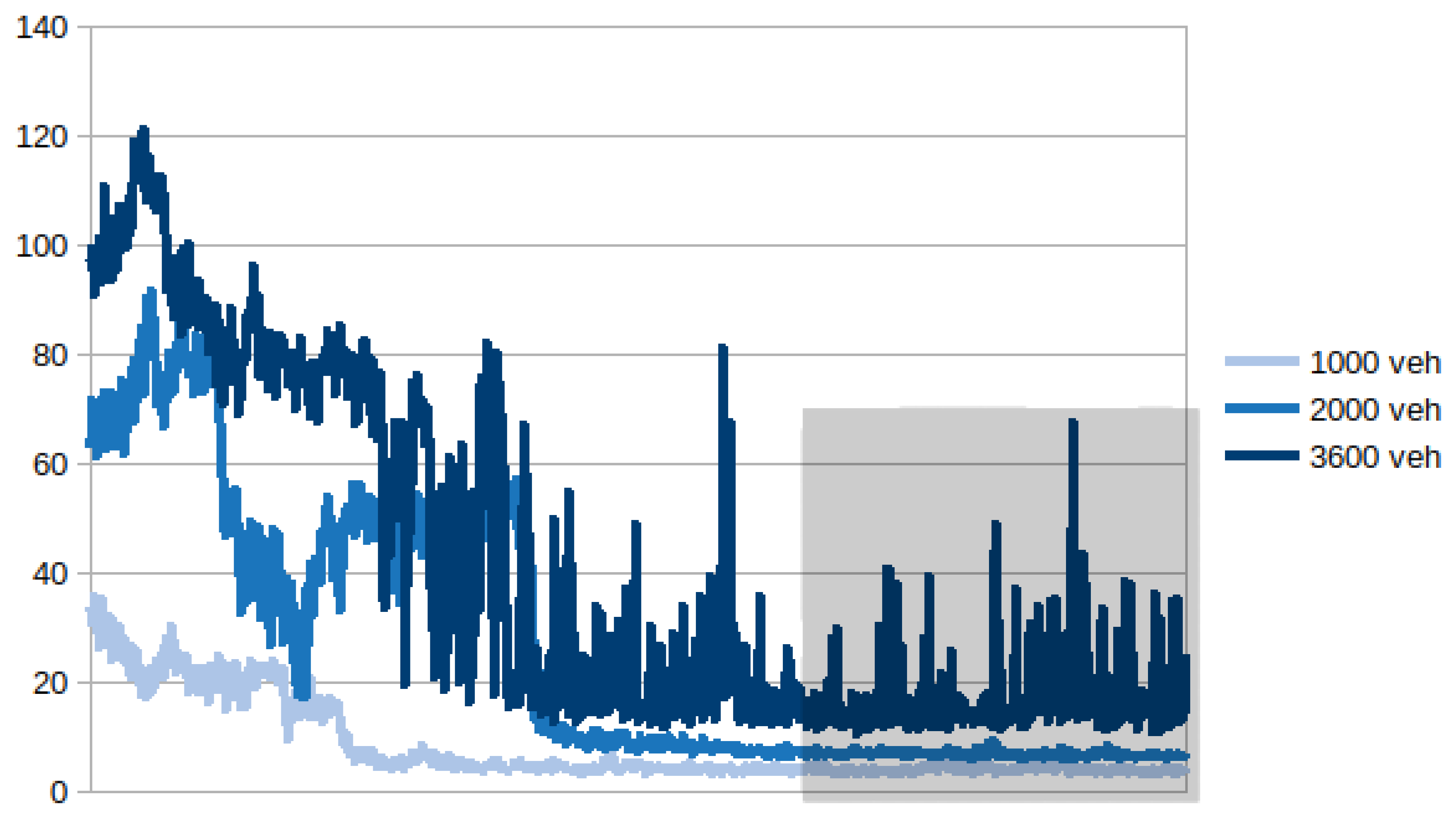
Figure 16 (shaded region).
Figure 16 shows that, when loaded with 1000 or 2000 vehicles, the achieved convergence stays stable while, when loaded with 3600 vehicles, the agents “keep struggling" even after reaching a balance among them, due to the excessive amount of vehicles circling on the traffic network.
4.3. Generalization
We performed further experiments to evaluate the generalization capability of the training process.
4.3.1. Random Learning
To test the tendency of the considered algorithms to focus on the signalized intersection dynamics, an attempt of training using totally random vehicle flows has been performed. This test differs from the previous ones as the random process seeds change at every simulation, instead of staying constant through the whole learning process. Even when adding only one vehicle per time step, no algorithm among those considered was able to achieve consistent positive results. On the Pasubio network with totally random training, only MA2C was able to optimize a policy within 10 attempts; this convergence is shown in
Figure 17.
When testing this solution on random test seeds, no better performance was achieved with respect to the pseudo-random case. This result has involved finding a “happy medium” that lies between the extreme of imposing completely random traffic conditions and the extreme of imposing a single seed for the entire training. The solution identified, which offers the optimal balance between the stability of the learning phase and the generality of the solution, involves keeping the seed constant for all episodes within the minibatch, and then varying it thereafter.
Table 6 shows that the MA2C performance after training on random traffic is slightly worse than when trained with pseudo-random traffic.
This experiment confirms that pseudo-random training is a well-balanced approach: its performance when tested with other random seeds (changing the vehicle distribution in terms of origin-destination pairs) shows that it avoids overfitting to spurious traffic circumstances while also presenting a more manageable learning problem than that posed by total-random training.
4.3.2. Policy Cross-Evaluation
This section presents another strategy to evaluate MA2C attitude towards overfitting. So far a certain solution has been evaluated only with its respective test cases; for instance, a policy learned with 2000 vehicles has been tested with the same number of vehicles (though in different vehicle distributions). This section presents the result of the learning step with varying vehicle loads. As an instance, MA2C has been tested to see how well the policy learned with 2000 vehicles performs with 3600 vehicles. These experiments have relevance as they contribute to help assessing the quality of pseudo-random training by allowing evaluating how much the agents are able to focus on the vehicle dynamics at their surroundings, resisting overfitting to other spurious features such as the vehicle load and distribution in time and space. The tables in the next sections report the results of the experiments.
Training MA2C with 2000 Vehicles:
Table 7 shows the results of MA2C compared to the greedy approach. Out of the six experiments reported, MA2C outperforms the greedy approach in five, with the notable exception of via Pasubio in a 2000 vehicle case. It is interesting that, though trained with 2000 vehicles, MA2C continues to perform well when dealing with 3600 vehicles, indicating that the learned policy does focus on the dynamics of the vehicle in the agents’ proximity. While MA2C failed to learn a policy for 4000 vehicles in 2000 time steps, the chaotic traffic related to this case can be alleviated by using the policy learned with 2000 vehicles, which performs slightly but noticeably better than Greedy.
Training MA2C with 3600 Vehicles:
Table 8 shows the results when training MA2C with 3600 vehicles. In all the experiments MA2C showed better performances than Greedy. It is noticeable that in the via Pasubio case, MA2C trained with 3600 performs better that MA2C trained with 2000 vehicles, even when tested with 2000 vehicles.
5. Results
It was found the need to position the algorithms within the framework of a Partially Observable Markov Decision Process (POMDP). The equations were subsequently reformulated within this framework, shedding light on which algorithms are truly compliant with the underlying Decision Process.
Further experimental results show that MA2C outperforms both IA2C and the Greedy approach by exhibiting a more robust behaviour when aiming to reduce the vehicle queues at signalized intersections.
For this purpose, attention is directed towards the A. Costa experiment featuring 2000 vehicles. As outlined in the preceding sections, the typical traffic simulation covers 3600 time steps.
In the first part of the simulation (time steps [0, 2000]) a vehicle is pseudo-randomly inserted on the map for each time step and follows a pseudo-random path.
In the second part of the simulation (time steps [2000, 3600]) no vehicle is inserted. Eventually, all the vehicles circulating on the map leave through one of the exit lanes or end their journey by reaching their destination.
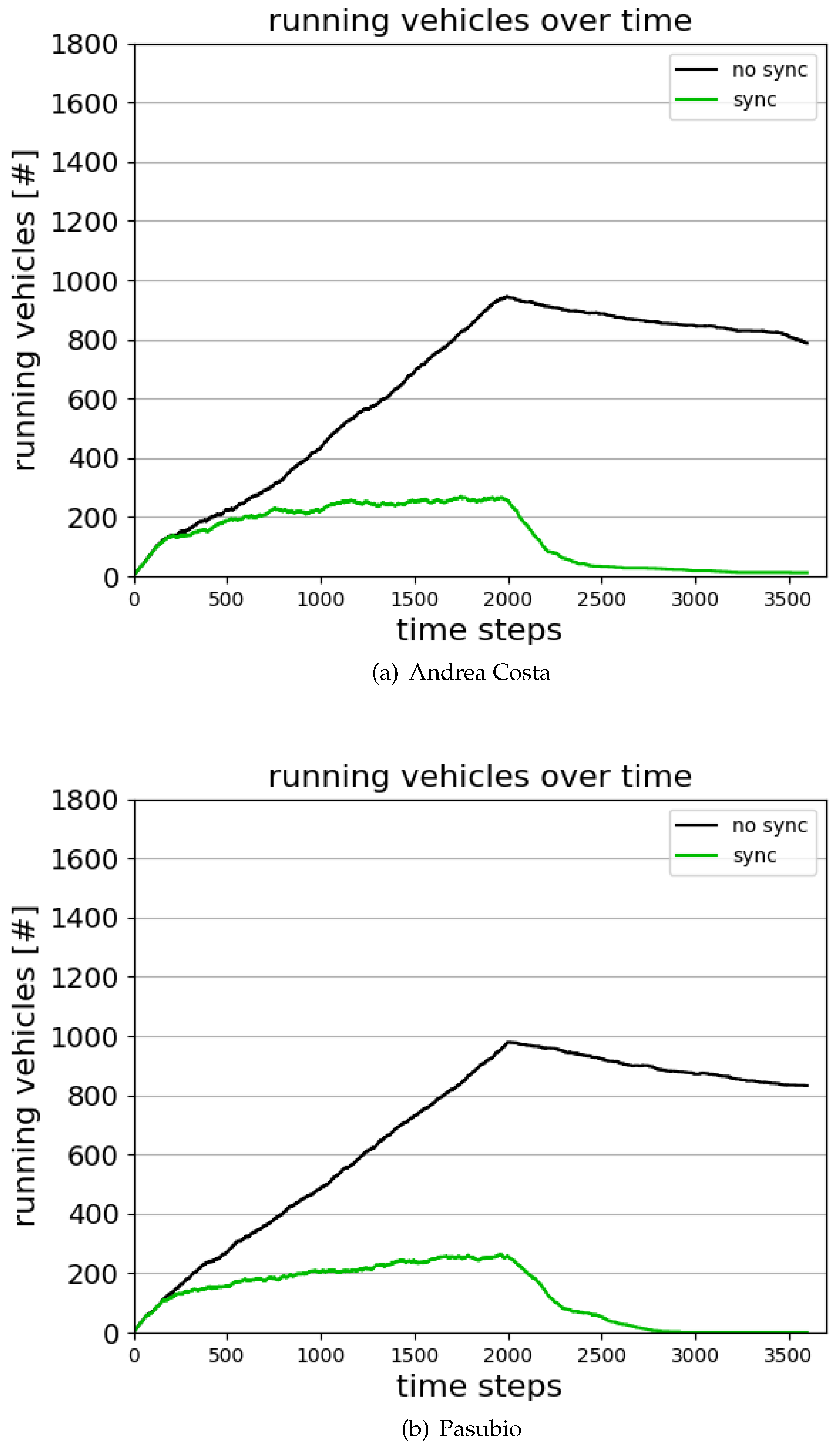
Figure 18 shows the number of running vehicles in the time span [0, 3600] for the cases Andrea Costa and Pasubio:
The curve referring to the beginning of the training ("no sync" in
Figure 18) - when a synchronization among the agents is yet to be achieved - shows that due to heavy queuing at the traffic lights, several vehicles stay on the road after time step 2000. In the graph, the curve keeps rising while vehicles are injected and tends to slowly decrease afterwards. When the network is trained ("sync" in
Figure 18), the amount of vehicles running fades quickly towards zero after time step 2000.
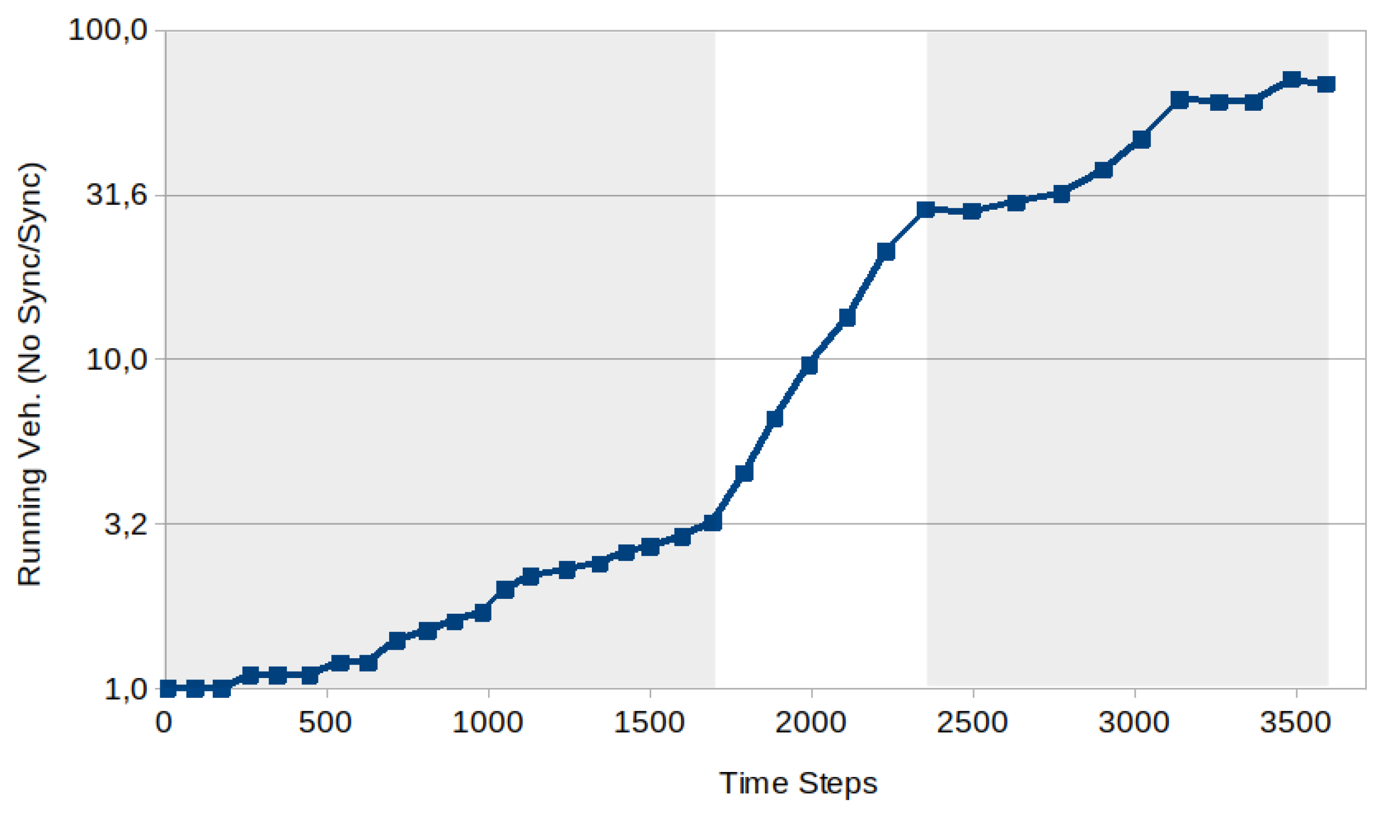
Figure 19 refers the Andrea Costa case and shows the behaviour of the ratio between the number of running vehicles with no sync over the same quantity in the sync case. The ratio increases and shows three distinct regions: a linear behaviour with two different slopes for
, an exponential behaviour for
, and a more irregular behaviour for
. The ratio at
is
, at
is
, while at
is
. The Pasubio case shows a similar pattern.
6. Conclusions
The development of multi-agent reinforcement learning methods for real-world problems represents a promising yet nascent research area [
35]. The complexities arise when attempting to strike a balance in a cooperative-competitive stochastic game. The aim of this study is to validate the theoretical framework of the algorithms proposed in [
13] and assess its effectiveness, robustness, and applicability in real-world scenarios. The theoretical framework of the algorithms has been critically reviewed and, given the overall state of partial observability, the Decision Process has been reframed within the context of a Partially Observable Markov Decision Process (POMDP), which is inherently non-Markovian. This is due to the observation space, which forces each agent to a subset of the total set of agents’ observations. The theory has been reformulated accordingly, as outlined in
Section 2.3 and
Section 2.4.1. This reformulation sheds light on the poorer performance of the class of Markovian algorithms (IQL-DNN, IQL-LR) compared to non-Markovian ones [
13]. The study confirms these findings, as detailed in
Section 3.3. Subsequently, the evaluation of IA2C and MA2C, compliant with the partially observable setting, takes place. In
Section 3.4, these algorithms undergo testing in two areas of Bologna (Italy) replicated in SUMO, a software tool for ATSC problems.
The analysis of the learning process and the comparison of results obtained by varying the number of vehicles indicate that MA2C is sufficiently effective. Specifically, it is demonstrated that in cases where the load is 2000 vehicles, MA2C generates a traffic decrease of a factor at the end of the simulation. These results are replicated in both the studied areas.
Examining the results obtained by training the system with pseudo-random vehicles and evaluating it with total random traffic, reveals that this training strategy is resistant to overfitting. This finding represents a significant step towards addressing real-world traffic problems with MARL algorithms, eliminating the need to know specific traffic flows in advance for training while resulting in adequate compromise between stability of the learning phase and generality of the solution.
The limitations of the evaluated algorithms become apparent at high traffic loads ( veh.); in these scenarios, both MA2C and IA2C perform comparably to a simple greedy approach. Future research may reveal whether there is a sharp transition to this behavior concerning the vehicle load.
Promising areas for future research include alternatives to LSTM cells, such as Echo State Networks (ESN) and Liquid State Machines, which can handle the chaotic behaviors of vehicle dynamics. These approaches also offer a faster training stage. Other directions aim to identify the dependency of the algorithm on the extent of the agents’ neighborhood and on specific settings such as the traffic network topology, the vehicle flow distributions, and origin-destination pairs.
As a final consideration, all simulations show that the process of balancing the agents’ actions is influenced by the number and interconnections among the agents (i.e., the signalized intersections), as well as by the traffic volume, which could be a typical situation in medium to large cities. To simplify the task, it may be beneficial to divide traffic network graphs into subgraphs. This strategy can be more efficiently implemented on less densely connected traffic networks, such as areas on the outskirts of cities, where agents tend to cluster in small groups.
Author Contributions
Paolo Fazzini: Project Administration, Conceptualization, Methodology, Formal Analysis, Investigation, Software, Validation, Visualization, Writing, Original draft preparation. Marco Montuori: Project Administration, Conceptualization, Formal Analysis, Writing Isaac Wheeler: Writing-Reviewing and Editing. Stefano Giagu: Supervision, Resources. Guido Caldarelli: Supervision, Resources. Marica De Lucia: Reviewing and Editing. Emilio Fortunato Campana: Resources. Francesco Petracchini: Supervision, Resources.
Acknowledgments
We thank Dr. Stefano Nolfi for his insightful advising. This research did not receive any specific grant from funding agencies in the public, commercial, or not-for-profit sectors. The authors have no competing interests to declare.
Glossary
| DP |
Decision Process. |
| IA2C |
Independent Advantage Actor Critic . |
| IQL-DNN |
Independent Q-Learning Deep Neural Network. |
| IQL-LR |
Independent Q-Learning Linear Regression. |
|
MA2C |
Multi-Agent Advantage Actor Critic . |
| MARL |
Multi-Agent Reinforcement Learning . |
| MDP |
Markovian Decision Process. |
| NMDP |
Non Markovian Decision Process. |
| OD |
Origin-Destination Matrix. |
| POMDP |
Partially Observable Markovian Decision Process. |
| RL |
Reinforcement Learning . |
| SUMO |
Simulation of Urban MObility . |
| TSC |
Traffic Signal Control. |
| Color should not be used for any figures in print. |
References
- Ghazali, W.; Zulkifli, C.N.; Ponrahono, Z. The Effect Of Traffic Congestion On Quality Of Community Life. European Proceedings of Multidisciplinary Sciences 2017. [Google Scholar] [CrossRef]
- Karimi, H.; Ghadirifaraz, B.; Shetab Boushehri, S.N.; Hosseininasab, S.M.; Rafiei, N. Reducing traffic congestion and increasing sustainability in special urban areas through one-way traffic reconfiguration. Trasportation 2022. [Google Scholar] [CrossRef]
- Jilani, U.; Asif, M.; Zia, M.Y.I.; Rashid, M.; Shams, S.; Otero, P. A Systematic Review on Urban Road Traffic Congestion. Wireless Personal Communications 2023. [Google Scholar] [CrossRef]
- Sen, S.; Li, H.; Khazanovich, L. Effect of climate change and urban heat islands on the deterioration of concrete roads. Results in Engineering 2022, 16, 100736. [Google Scholar] [CrossRef]
- Liu, D.; Li, L. A traffic light control method based on multi-agent deep reinforcement learning algorithm. Nature 2023, 13. [Google Scholar] [CrossRef] [PubMed]
- Sutton, R.S.; Barto, A.G. Reinforcement learning: an introduction; Adaptive computation and machine learning, MIT Press.
- Huang, J.; Cui, Y.; Zhang, L.; Tong, W.; Shi, Y.; Liu, Z. An Overview of Agent-Based Models for Transport Simulation and Analysis. Journal of Advanced Transportation 2022, 2022, 1–17. [Google Scholar] [CrossRef]
- Shoham, Y.; Leyton-Brown, K. Multiagent Systems: Algorithmic, Game-Theoretic, and Logical Foundations; Cambridge University Press, 2008. [CrossRef]
- Miletić, M.; Ivanjko, E.; Gregurić, M.; Kušić, K. A review of reinforcement learning applications in adaptive traffic signal control. IET Intelligent Transport Systems 2022, 16, n. [Google Scholar] [CrossRef]
- Chu, T.; Chinchali, S.; Katti, S. Multi-agent Reinforcement Learning for Networked System Control. 2020; arXiv:cs.LG/2004.01339. [Google Scholar]
- Jiang, Q.; Qin, M.; Shi, S.; Sun, W.; Zheng, B. Multi-Agent Reinforcement Learning for Traffic Signal Control through Universal Communication Method. 2022; arXiv:cs.AI/2204.12190. [Google Scholar]
- Wong, A.; Bäck, T.; Kononova, A.V.; Plaat, A. Deep multiagent reinforcement learning: challenges and directions.
- Chu, T.; Wang, J.; Codecà, L.; Li, Z. Multi-Agent Deep Reinforcement Learning for Large-scale Traffic Signal Control. 2019; arXiv:cs.LG/1903.04527. [Google Scholar]
- Lopez, P.A.; Wiessner, E.; Behrisch, M.; Bieker-Walz, L.; Erdmann, J.; Flotterod, Y.P.; Hilbrich, R.; Lucken, L.; Rummel, J.; Wagner, P. Microscopic Traffic Simulation using SUMO. 2018 21st International Conference on Intelligent Transportation Systems (ITSC). IEEE, pp. 2575–2582. [CrossRef]
- Hunt, P.; Robertson, D.; Bretherton, R.D.; Royle, M. THE SCOOT ON-LINE TRAFFIC SIGNAL OPTIMISATION TECHNIQUE. Traffic engineering and control 1982, 23. [Google Scholar]
- Luk, J. Two traffic responsive area traffic control methods: SCAT and SCOOT. 1983.
- Gokulan, B.P.; Srinivasan, D. Distributed Geometric Fuzzy Multiagent Urban Traffic Signal Control. 11, 714–727. [CrossRef]
- Teodorović, D. Swarm intelligence systems for transportation engineering: Principles and applications. 16, 651–667. [CrossRef]
- Lee, J.; Abdulhai, B.; Shalaby, A.; Chung, E.H. Real-Time Optimization for Adaptive Traffic Signal Control Using Genetic Algorithms. Journal of Intelligent Transportation Systems 2005, 9, 111–122. [Google Scholar] [CrossRef]
- Huang, J.; Cui, Y.; Zhang, L.; Tong, W.; Shi, Y.; Liu, Z. An Overview of Agent-Based Models for Transport Simulation and Analysis. Journal of Advanced Transportation 2022, 2022, 1–17. [Google Scholar] [CrossRef]
- Wu, C.; Ma, Z.; Kim, I. Multi-Agent Reinforcement Learning for Traffic Signal Control: Algorithms and Robustness Analysis. 2020, pp. 1–7. [CrossRef]
- Huang, J.; Cui, Y.; Zhang, L.; Tong, W.; Shi, Y.; Liu, Z. An Overview of Agent-Based Models for Transport Simulation and Analysis. Journal of Advanced Transportation 2022, 2022, 1–17. [Google Scholar] [CrossRef]
- Lample, G.; Chaplot, D.S. Playing FPS Games with Deep Reinforcement Learning. Proceedings of the Thirty-First AAAI Conference on Artificial Intelligence, February 4-9, 2017, San Francisco, California, USA; Singh, S.; Markovitch, S., Eds. AAAI Press, pp. 2140–2146.
- Williams, R.J. Simple statistical gradient-following algorithms for connectionist reinforcement learning. Machine Learning 1992, 8, 229–256. [Google Scholar] [CrossRef]
- Mnih, V.; Badia, A.P.; Mirza, M.; Graves, A.; Lillicrap, T.P.; Harley, T.; Silver, D.; Kavukcuoglu, K. Asynchronous Methods for Deep Reinforcement Learning. CoRR 2016, abs/1602.01783. arXiv:1602.01783.
- Bieker, L.; Krajzewicz, D.; Morra, A.P.; Michelacci, C.; Cartolano, F. Traffic simulation for all: A real world traffic scenario from the city of Bologna. Lecture Notes in Control and Information Sciences 2015, 13, 47–60. [Google Scholar] [CrossRef]
- Zhang, C.; Vinyals, O.; Munos, R.; Bengio, S. A Study on Overfitting in Deep Reinforcement Learning. 2018; arXiv:cs.LG/1804.06893. [Google Scholar]
- Kolat, M.; Kővári, B.; Bécsi, T.; Aradi, S. Multi-Agent Reinforcement Learning for Traffic Signal Control: A Cooperative Approach. Sustainability 2023, 15. [Google Scholar] [CrossRef]
- Bera, S.; Rao, K.V. Estimation of origin-destination matrix from traffic counts: The state of the art. European Transport Trasporti Europei 2011, 49, 2–23. [Google Scholar]
- Ronca, A.; Paludo Licks, G.; De Giacomo, G. Markov Abstractions for PAC Reinforcement Learning in Non-Markov Decision Processes 2022.
- Grosnit, A.; Cai, D.; Wynter, L. Decentralized Deterministic Multi-Agent Reinforcement Learning. 2021; arXiv:cs.LG/2102.09745. [Google Scholar]
- Zhang, K.; Yang, Z.; Liu, H.; Zhang, T.; Basar, T. Fully Decentralized Multi-Agent Reinforcement Learning with Networked Agents. Proceedings of the 35th International Conference on Machine Learning; Dy, J.; Krause, A., Eds. PMLR, 2018, Vol. 80, Proceedings of Machine Learning Research, pp. 5872–5881.
- Zhu, R.; Ding, W.; Wu, S.; Li, L.; Lv, P.; Xu, M. Auto-learning communication reinforcement learning for multi-intersection traffic light control. Knowledge-Based Systems 2023, 275, 110696. [Google Scholar] [CrossRef]
- Zhang, K.; Yang, Z.; Başar, T. , K.G.; Wan, Y.; Lewis, F.L.; Cansever, D., Eds.; Springer International Publishing: Cham, 2021; pp. 321–384. doi:10.1007/978-3-030-60990-0_12.Algorithms. In Handbook of Reinforcement Learning and Control; Vamvoudakis, K.G., Wan, Y., Lewis, F.L., Cansever, D., Eds.; Springer International Publishing: Cham, 2021; Springer International Publishing: Cham, 2021; pp. 321–384. [Google Scholar] [CrossRef]
- Irpan, A. Deep Reinforcement Learning Doesn’t Work Yet. 2018. Available online: https://www.alexirpan.com/2018/02/14/rl-hard.html.
| 1 |
The latter two Q-learning based RL algorithms differ from each other in the way they fit the Q-function, i.e., by linear regression or by a deep neural network [ 13] |
| 2 |
SUMO [ 14] is a micro-traffic simulator capable of simulating traffic dynamics |
| 3 |
Each agent observes the traffic flow in its proximity and its neighboring agents proximity; see Section 2.2.1 for a formal definition |
| 4 |
In accordance with the literature on the subject, this work designates this quantity as the reward, notwithstanding the fact that the length of a vehicle queue is given (and perceived) as a penalty. |
| 5 |
Strategy and policy refer to similar entities. The former is more common in game theory, while the latter is more popular in reinforcement learning; in this work these two terms are used interchangeably |
| 6 |
To lighten the notation, in some cases the dependence from will be omitted if clear from the context |
| 7 |
In [ 13] and are referred as the frozen state-value and policy to include in the development an eventual frozen set of parameters staying constant during multiple learning steps. We prefer to avoid this terminology as in the implementation reported here the parameters are updated after each learning step |
| 8 |
The MA2C spatial discount factor highlights the competitive character of the mixed cooperative-competitive game among the agents, as opposed to IA2C which is purely cooperative. |
| 9 |
Root Mean Squared Propagation is an unpublished algorithm first proposed by Geoffrey Hinton in the Coursera course “Neural Network for Machine Learning”, lecture 6, 2018 |
| 10 |
For all the tests and the totally random learning experiment, the seeds used are: 10400, 20200, 31000, 3101, 122, 42, 20200, 33333. |
| 11 |
In the main experiment of [ 13], on the city of Monaco, vehicle flows on specific roads are predetermined; some randomness is allowed, but it affects only a vehicle’s position on the starting road, while its route to its destination is deterministic. |
| 12 |
In [ 13] a good behavior of IQL-DNN and IQL-LR is reported only for basic (unrealistic) experiments such as regular grids; in fact in Figure 9 and 10 in [ 13], they have been omitted due to their poor performance with a real traffic network. IQL based approaches are also reported to perform well in [ 28], where a 6 agents squared lattice traffic grid is adopted and in [ 28] with a 4 agent squared lattice. |
| 13 |
This quantity includes the contributions of all the signalized intersections and is further averaged over the episode length; it will be referred to simply as "average queue" in the next sections. |
| 14 |
Similarly to all the other experiments reported, every learning process has been repeated ten times, with similar results. |
| 15 |
As highlighted in Section 2.3, the environment is partially observable (non-markovian). IQL-DNN and IQL-LR rely on the present information to forecast one step ahead so they are unable to exploit information from past time steps. |
| 16 |
For a more in-depth exploration of MA2C and IA2C’s perception of the environment, please refer to Section 2.3. This section delves into the reasons why the Decision Process should be reformulated within the context of POMDP, which represents a broader class of Decision Processes compared to RDP. |
| 17 |
is the Kullback–Leibler divergence |
Figure 1.
Traffic network: the shaded round spots (light blue) reference the signalized intersections (agents); their respective crossroads, contained in the round spots, are highlighted in dark (green) colour; the crossroads not controlled by traffic lights are highlighted in light (yellow) color.
Figure 1.
Traffic network: the shaded round spots (light blue) reference the signalized intersections (agents); their respective crossroads, contained in the round spots, are highlighted in dark (green) colour; the crossroads not controlled by traffic lights are highlighted in light (yellow) color.
Figure 2.
Agent i Reward and Observation in MA2C, IA2C, IQL-DNN and IQL-LR. The dotted rounded rectangle represents a traffic network; the filled circle is agent i while the empty circles the other agents; the dotted circle represents agent i’s neighborhood.
Figure 2.
Agent i Reward and Observation in MA2C, IA2C, IQL-DNN and IQL-LR. The dotted rounded rectangle represents a traffic network; the filled circle is agent i while the empty circles the other agents; the dotted circle represents agent i’s neighborhood.
Figure 3.
General Scheme: while seeking for an optimal Policy, Loss Minimization requires a repeated sequence of state-action-reward-next state steps.
Figure 3.
General Scheme: while seeking for an optimal Policy, Loss Minimization requires a repeated sequence of state-action-reward-next state steps.
Figure 4.
ANN Scheme of IA2C and MA2C
Figure 4.
ANN Scheme of IA2C and MA2C
Figure 7.
Average Queue while learning for IQL-DNN for the cases Andrea Costa and Pasubio.
Figure 7.
Average Queue while learning for IQL-DNN for the cases Andrea Costa and Pasubio.
Figure 8.
Average Queue while learning for IQL-LR for the cases Andrea Costa and Pasubio.
Figure 8.
Average Queue while learning for IQL-LR for the cases Andrea Costa and Pasubio.
Figure 9.
Andrea Costa, average queue, 2000 veh, IA2C and MA2C: training steps are shown on the horizontal axis.
Figure 9.
Andrea Costa, average queue, 2000 veh, IA2C and MA2C: training steps are shown on the horizontal axis.
Figure 10.
Andrea Costa, average queue, 3600 veh, IA2C and MA2C: training steps are shown on the horizontal axis.
Figure 10.
Andrea Costa, average queue, 3600 veh, IA2C and MA2C: training steps are shown on the horizontal axis.
Figure 11.
Pasubio IA2C and MA2C: average queue when loading the traffic network with 2000 vehicles in pseudo-random traffic conditions.
Figure 11.
Pasubio IA2C and MA2C: average queue when loading the traffic network with 2000 vehicles in pseudo-random traffic conditions.
Figure 12.
Pasubio, IA2C and MA2C: average queue when loading the traffic network with 3600 vehicles in pseudo-random traffic conditions.
Figure 12.
Pasubio, IA2C and MA2C: average queue when loading the traffic network with 3600 vehicles in pseudo-random traffic conditions.
Figure 13.
MA2C: average queue during training when loading the traffic network with 4000 vehicles in the time interval [0-2000], in pseudo-random traffic conditions.
Figure 13.
MA2C: average queue during training when loading the traffic network with 4000 vehicles in the time interval [0-2000], in pseudo-random traffic conditions.
Figure 14.
A. Costa learning graphs showing the evolution in time of seven agents’ loss () and their accrued Reward when the traffic network is loaded with 2000 vehicles. The left (red) shaded region highlights the inconsistency issue: at the beginning of the shaded region agent is slightly unstable (while the other agents appear to be close to a relative balance) and eventually drags away the other agents from their converging path. In the (green) shaded region on the right, instead, all the agents appear to move together towards a common relative minimum.
Figure 15.
Learning stability while training with the Andrea Costa Traffic Network, loaded with 2000 veh.
Figure 15.
Learning stability while training with the Andrea Costa Traffic Network, loaded with 2000 veh.
Figure 16.
Loss behaviour in the A. Costa case (1000, 2000 and 3600 veh). When loaded with 1000 or 2000 vehicles, the achieved convergence stays stable while, when loaded with 3600 veh, the agents “keep struggling" even after reaching a balance among them.
Figure 16.
Loss behaviour in the A. Costa case (1000, 2000 and 3600 veh). When loaded with 1000 or 2000 vehicles, the achieved convergence stays stable while, when loaded with 3600 veh, the agents “keep struggling" even after reaching a balance among them.
Figure 17.
Pasubio, MA2C: average queue when loading the traffic network with 3600 vehicles in random traffic conditions.
Figure 17.
Pasubio, MA2C: average queue when loading the traffic network with 3600 vehicles in random traffic conditions.
Figure 18.
Running vehicles over time
Figure 18.
Running vehicles over time
Figure 19.
The figure, plotted on a semi-logarithmic scale (y-axis on a logarithmic scale and x-axis on a linear scale), represents the ratio of running vehicles at time
t in the case of no synchronization over the same quantity in the synchronization case (black and green curves in
Figure 18). The ratio increases and shows three distinct regions: a linear behaviour with two different slopes for
, an exponential behaviour for
, and a more irregular behaviour for
. The ratio at
is
, at
is
, while at
is
. In the case where synchronization is not implemented, the number of running vehicles is approximately 70 times greater compared to the synchronized scenario at the end of the episode.
Table 1.
IA2C and MA2C Settings.
Table 1.
IA2C and MA2C Settings.
| Par. |
Value |
Description |
|
0.9 |
spatial weighting factor |
|
3600 [s] |
total period of simulated traffic |
|
t |
5 [s] |
interaction time between each agent and the traffic environment |
|
2 [s] |
yellow time |
|
2000,3600 [veh] |
total number of vehicles |
|
0.99 |
discount factor, controlling how much expected future reward is weighted |
|
|
coefficient for used for gradient descent optimization |
|
|
coefficient for
|
|
40 |
size of the batch buffer |
|
0.01 |
parameter to balance the entropy loss of policy to encourage early-stage exploration |
Table 2.
Average Queue Test, Andrea Costa, 2000 veh.
Table 2.
Average Queue Test, Andrea Costa, 2000 veh.
| Test |
1 |
2 |
3 |
4 |
5 |
6 |
7 |
8 |
Ave |
Std |
| MA2C |
6.55 |
5.81 |
6.26 |
5.66 |
6.33 |
5.90 |
5.98 |
6.08 |
6.07 |
0.28 |
| IA2C |
8.38 |
8.43 |
8.36 |
8.15 |
7.8 |
8.09 |
8.7 |
8.75 |
8.33 |
0.30 |
| Greedy |
25.29 |
18.52 |
23.19 |
17.58 |
20.79 |
17.36 |
18.52 |
24.14 |
20.67 |
2.95 |
Table 3.
Average Queue Test, A. Costa 3600 veh.
Table 3.
Average Queue Test, A. Costa 3600 veh.
| Test |
1 |
2 |
3 |
4 |
5 |
6 |
7 |
8 |
Ave |
Std |
| MA2C |
11.59 |
11.70 |
12.72 |
11.60 |
10.88 |
11.12 |
10.84 |
11.64 |
11.51 |
0.56 |
| IA2C |
18.89 |
18.88 |
20.72 |
19.55 |
17.56 |
19.75 |
18.06 |
19.25 |
19.08 |
0.92 |
| Greedy |
27.96 |
28.94 |
33.18 |
29.19 |
27.96 |
38.51 |
30.46 |
31.64 |
30.98 |
3.31 |
Table 4.
Average Queue Test, Pasubio, 2000 veh.
Table 4.
Average Queue Test, Pasubio, 2000 veh.
| Test |
1 |
2 |
3 |
4 |
5 |
6 |
7 |
8 |
Ave |
Std |
| MA2C |
17.56 |
24.73 |
29.5 |
30.36 |
29.49 |
21.93 |
36.53 |
22.44 |
26.57 |
5.63 |
| IA2C |
61.22 |
79.24 |
70.99 |
73.06 |
70.06 |
101.67 |
57.67 |
29.47 |
67.92 |
19.16 |
| Greedy |
10.61 |
15.14 |
19.89 |
15.76 |
14.14 |
22.58 |
15.14 |
20.88 |
16.77 |
3.73 |
Table 5.
Average Queue Test, Pasubio 3600 veh.
Table 5.
Average Queue Test, Pasubio 3600 veh.
| Test |
1 |
2 |
3 |
4 |
5 |
6 |
7 |
8 |
Ave |
Std |
| MA2C |
32.03 |
33.06 |
41.25 |
35.66 |
28.20 |
35.82 |
31.16 |
33.42 |
33.82 |
3.63 |
|
Greedy: |
26.71 |
37.78 |
37.44 |
35.36 |
28.60 |
80.66 |
37.78 |
76.23 |
45.07 |
19.70 |
Table 6.
MA2C, Average Queue Test, Pasubio, 3600 veh., trained with pseudo-random and random traffic.
Table 6.
MA2C, Average Queue Test, Pasubio, 3600 veh., trained with pseudo-random and random traffic.
| Test |
1 |
2 |
3 |
4 |
5 |
6 |
7 |
8 |
Ave |
Std |
| P. Random |
32.03 |
33.06 |
41.25 |
35.66 |
28.20 |
35.82 |
31.16 |
33.42 |
33.82 |
3.63 |
| Random |
31.54 |
35.45 |
59.39 |
33.29 |
28.73 |
49.50 |
34.56 |
40.45 |
39.11 |
9.71 |
Table 7.
Average Queue Cross Test, MA2C trained with 2000 vehicles.
Table 7.
Average Queue Cross Test, MA2C trained with 2000 vehicles.
| A. Costa |
|---|
| Testing: 2000 veh. |
Ave |
Std |
| MA2C |
6.55 |
5.81 |
6.26 |
5.66 |
6.33 |
5.90 |
5.98 |
6.08 |
6.07 |
0.28 |
| Greedy |
25.29 |
18.52 |
23.19 |
17.58 |
20.79 |
17.36 |
18.52 |
24.14 |
20.67 |
2.95 |
| Testing: 3600 veh. |
Ave |
Std |
| MA2C |
9.20 |
8.9 |
28.54 |
20.69 |
9.16 |
8.73 |
8.86 |
9.09 |
12.90 |
7.05 |
| Greedy |
27.96 |
28.94 |
33.18 |
29.19 |
27.96 |
38.51 |
30.46 |
31.64 |
30.98 |
3.31 |
| Testing: 4000 veh. |
Ave |
Std |
| MA2C |
133.3 |
141.6 |
143.6 |
140.2 |
131.9 |
144.0 |
140.3 |
138.3 |
139.1 |
4.17 |
| Greedy |
163.2 |
161.15 |
168.3 |
163.1 |
154.9 |
166.6 |
161.1 |
162.5 |
162.6 |
3.76 |
| Pasubio |
| Testing: 2000 veh. |
Ave |
Std |
| MA2C |
17.56 |
24.73 |
29.5 |
30.36 |
29.49 |
21.93 |
36.53 |
22.44 |
26.57 |
5.63 |
| Greedy |
10.61 |
15.14 |
19.89 |
15.76 |
14.14 |
22.58 |
15.14 |
20.88 |
16.77 |
3.73 |
| Testing: 3600 veh. |
Ave |
Std |
| MA2C |
32.03 |
33.06 |
41.25 |
35.66 |
28.20 |
35.82 |
31.16 |
33.42 |
33.82 |
3.63 |
| Greedy |
26.71 |
37.78 |
37.44 |
35.36 |
28.60 |
80.66 |
37.78 |
76.23 |
45.07 |
19.70 |
| Testing: 4000 veh. |
Ave |
Std |
| MA2C |
255.9 |
240.7 |
241.6 |
267.4 |
261.6 |
255.4 |
248.8 |
250.7 |
252.7 |
8.65 |
| Greedy |
257.3 |
251.3 |
259.4 |
273.0 |
275.0 |
263.2 |
251.4 |
262.4 |
261.6 |
8.25 |
Table 8.
Average Queue Cross Test, MA2C trained with 3600 vehicles.
Table 8.
Average Queue Cross Test, MA2C trained with 3600 vehicles.
| A. Costa |
|---|
| Testing: 2000 veh. |
Ave |
Std |
| MA2C |
7.78 |
7.22 |
7.05 |
7.92 |
7.05 |
7.32 |
7.20 |
7.16 |
7.33 |
0.31 |
| Greedy |
25.29 |
18.52 |
23.19 |
17.58 |
20.79 |
17.36 |
18.52 |
24.14 |
20.67 |
2.95 |
| Testing: 3600 veh. |
Ave |
Std |
| MA2C |
10.84 |
11.59 |
17.59 |
11.70 |
12.90 |
12.72 |
11.60 |
10.88 |
12.48 |
2.05 |
| Greedy |
27.96 |
28.94 |
33.18 |
29.19 |
27.96 |
38.51 |
30.46 |
31.64 |
30.98 |
3.31 |
| Testing: 4000 veh. |
Ave |
Std |
| MA2C |
132.9 |
142.4 |
139.3 |
144.8 |
137.3 |
144.7 |
140.5 |
140.0 |
140.2 |
3.69 |
| Greedy |
163.2 |
161.15 |
168.3 |
163.1 |
154.9 |
166.6 |
161.1 |
162.5 |
162.6 |
3.76 |
| Pasubio |
| Testing: 2000 veh. |
Ave |
Std |
| MA2C |
14.82 |
17.00 |
18.44 |
18.09 |
21.20 |
22.57 |
20.60 |
20.84 |
19.20 |
2.39 |
| Greedy |
10.61 |
15.14 |
19.89 |
15.76 |
14.14 |
22.58 |
15.14 |
20.88 |
16.77 |
3.73 |
| Testing: 3600 veh. |
Ave |
Std |
| MA2C |
23.10 |
28.91 |
22.51 |
23.66 |
22.09 |
38.23 |
25.16 |
33.42 |
30.6 |
5.53 |
| Greedy |
26.71 |
37.78 |
37.44 |
35.36 |
28.60 |
80.66 |
37.78 |
76.23 |
45.07 |
19.70 |
| Testing: 4000 veh. |
Ave |
Std |
| MA2C |
241.5 |
248.8 |
244.1 |
272.9 |
259.2 |
248.6 |
250.9 |
253.5 |
252.5 |
9.26 |
| Greedy |
257.3 |
251.3 |
259.4 |
273.0 |
275.0 |
263.2 |
251.4 |
262.4 |
261.6 |
8.25 |
|
Disclaimer/Publisher’s Note: The statements, opinions and data contained in all publications are solely those of the individual author(s) and contributor(s) and not of MDPI and/or the editor(s). MDPI and/or the editor(s) disclaim responsibility for any injury to people or property resulting from any ideas, methods, instructions or products referred to in the content. |
© 2024 by the authors. Licensee MDPI, Basel, Switzerland. This article is an open access article distributed under the terms and conditions of the Creative Commons Attribution (CC BY) license (http://creativecommons.org/licenses/by/4.0/).