
Submitted:
09 August 2025
Posted:
12 August 2025
You are already at the latest version
Abstract
Soundscape monitoring has become an increasingly important tool for studying ecological processes and supporting habitat conservation. While many recent advances focus on identifying species through supervised learning, there is growing interest in understanding the soundscape as a whole considering patterns that go beyond individual vocalizations. This broader view requires unsupervised approaches capable of capturing meaningful structures related to temporal dynamics, frequency content, spatial distribution, and ecological variability. In this study, we present a fully unsupervised framework for analyzing large-scale soundscape data using deep learning. We applied a convolutional autoencoder (Soundscape-Net) to extract acoustic representations from over 60,000 recordings collected across a grid-based sampling design in the Rey Zamuro Reserve, Colombia. Dimensionality reduction methods (UMAP and PaCMAP) were used to project the learned features, followed by clustering with KMeans and DBSCAN to explore latent acoustic structures. To interpret and validate the resulting clusters, we combined multiple strategies: spatial mapping through interpolation, analysis of acoustic index variance to understand cluster structure, and graph-based connectivity analysis to identify ecological relationships between recording sites. Our results demonstrate that this approach can uncover both local and broad-scale patterns in the soundscape, providing a flexible and interpretable pathway for unsupervised ecological monitoring.
Keywords:
autoencoders
; deep learning
; ecoacoustics
; embeddings
; feature projections
; soundscape patterns
; unsupervised learning
1. Introduction
In recent years, the study of soundscapes has emerged as a powerful tool for ecological monitoring and environmental assessment. A soundscape is defined as the collection of biophonic, geophonic, and anthropophonic sounds that characterize a given environment [1]. Through passive acoustic monitoring, researchers can gather continuous, non-invasive, and cost-effective information about ecosystems, including biological activity, species richness, and anthropogenic disturbance [2]. Unlike traditional biodiversity surveys that are often limited by spatial or temporal constraints, acoustic methods enable long-term sampling across large areas and can reveal patterns that would otherwise remain undetected. These advantages have contributed to the growing adoption of soundscape analysis in conservation programs, landscape-scale monitoring efforts, and biodiversity assessments [3]. As acoustic technologies and computational tools continue to improve, soundscapes offer increasing potential for understanding the dynamics and health of ecosystems on spatial and temporal scales.
Recent developments in machine learning have significantly improved the ability to analyze ecoacoustic data [2,4], particularly in tasks involving species detection and classification. Supervised learning techniques, especially those based on deep neural networks, have enabled the automatic identification of animal vocalizations from large volumes of acoustic recordings [4,5]. Notably, tools such as BirdNET [6], which use convolutional neural networks trained on expert-labeled datasets, have achieved high accuracy in the identification of numerous species of birds in different environments. These models have facilitated large scale biodiversity monitoring and made it possible to study specie specific patterns with high temporal resolution [7,8]. Despite these advances, many existing approaches focus primarily on taxonomic classification, often ignoring the broader acoustic structure of the landscape and the contextual information embedded in non-biological or unclassified sounds. This narrow focus limits the ecological interpretation of soundscapes and restricts the ability to assess ecosystem-level properties. However, the acoustic environment encodes more than just the presence of species or vocal activity. Soundscapes reflect the structure and function of ecosystems as a whole, including spatial patterns, temporal dynamics, and environmental stressors [9,10,11]. Attributes such as habitat connectivity, land-use heterogeneity, and ecosystem degradation can be inferred from the composition and variability of acoustic signals over time and space. These broader patterns are essential for understanding ecological processes, especially in landscapes undergoing rapid change. Yet, studies that treat the soundscape as a complex and integrated ecological signal remain relatively scarce. Most existing research has prioritized species-level outcomes, leaving a gap in our understanding of how acoustic patterns relate to landscape structure and ecosystem health. In this study, we address this gap by comparing multiple methodological pipelines that combine dimensionality reduction and unsupervised clustering for large-scale soundscape characterization. Our goal is to explore how these approaches reveal spatial organization in the acoustic environment and to provide tools for interpreting the composition and distribution of clusters from an ecological perspective.
Our work is based on and motivated by recent efforts to explore soundscape patterns through unsupervised analysis. For example, [12] used acoustic indices to perform spatial exploration of soundscapes within the same study area examined here. Their work emphasized the value of unsupervised learning and evaluated clustering outputs through comparisons with species detections, spectrograms, and the spatial distribution of acoustic indices, highlighting how soundscape-level structure can emerge without relying on taxonomic annotation. Similarly, [13] proposed an unsupervised framework that leverages passive acoustic monitoring data and network inference to examine acoustic heterogeneity across landscapes. By characterizing biophonic patterns through the use of sonotypes they constructed site level profiles and applied graphical models to infer ecological interactions. Their graph-based approach allowed them to represent similarities among sites and capture acoustic diversity in heterogeneous environments.
On the other hand, although autoencoders have been widely adopted in other fields such as bioinformatics [14], cybersecurity [15], anomaly detection [16], and even remote sensing and landscape monitoring applications [17,18], they remain relatively underused in ecoacoustics. Notable exceptions include the work by [19], who proposed a vector-quantized autoencoder for generating synthetic audio of underrepresented species, and [20], one of the earliest studies to explore autoencoders as an alternative to acoustic indices for clustering short audio recordings. Additionally, in our previous work [21], we evaluated unsupervised learning using a variational autoencoder in comparison with cepstral coefficients and a convolutional architecture known as KiwiNet, highlighting the potential of deep unsupervised representations for soundscape analysis. However, our current work distinguishes itself from the studies mentioned above and from our previous research in several key aspects: (i) we conduct an in-depth evaluation of the dimensionality reduction and clustering stages, emphasizing the importance of parameter selection through both quantitative metrics and qualitative analyses; (ii) we thoroughly assess the relationship between the discovered patterns and ecological attributes derived from metadata, particularly emphasizing spatial structure; and (iii) we propose a novel methodology to identify acoustically connected geographic locations based on the similarity of their recordings, an aspect that, to our knowledge, has not been explicitly addressed in previous ecoacoustic studies.
2. Materials and Methods
2.1. Dataset Description
The dataset used in this study was obtained from passive acoustic recordings collected within the Rey Zamuro and Matarredonda Private Nature Reserve, located in the village of La Novilla, San Martín municipality, Meta Department, Colombia (approximately at N, W). Established in 1993, the reserve spans an area of 6,000 hectares, predominantly composed of natural savannas and introduced pastures (around 60 %), while the remaining 40 % consists of forest cover [12]. The area is part of the tropical humid foothill biome of the Meta region, with elevations ranging between 260 and 300 meters above sea level. It lies near the confluence of three hydrographic basins: Caños Cumaral, Chunaipo, and Camoa [22].
The reserve harbors a variety of ecosystems. Forested areas include gallery or riparian forests that line streams and rivers, functioning as critical biological corridors and refuges for fauna within the savanna matrix. In particular, approximately 1,200 hectares of dense, well-conserved forest are found in the Matarredonda sector. Seasonally flooded forests of the várzea or igapó type are also present and are ecologically important, especially for primate species that frequently utilize canopy strata between 12 and 18 meters in height [23].
The savanna complex consists of multiple formations, including ecologically significant
morichales—wetlands dominated by the palm Mauritia flexuosa—which are known to support a wide variety of fauna. Acoustic monitoring was also conducted in other non-forest habitats such as dense shrublands, grasslands, and pasturelands. The ecological interface between open savanna habitats and forest patches, particularly the gallery forests that cut across the landscape, is regarded as a key component in sustaining regional biodiversity and ecological functionality.
The climate in this region is classified as humid tropical, with a mean annual temperature of 25.6 ∘C and an average annual precipitation of approximately 2,513 mm. Sunrise occurs around 6:06 a.m., and sunset around 6:05 p.m., resulting in roughly 12 hours of daylight year-round.
The acoustic recordings were obtained through a grid-based sampling design, deploying 94 AudioMoth devices (versions 1.0.0 to 1.2.0) spaced 200 m apart. Devices were mounted at a standardized height of 1.5 m above ground, enclosed in Ziploc bags for protection, and powered by AA alkaline batteries, using 32 GB Sandisk Extreme memory cards for data storage. Recordings were captured in mono at a sampling rate of 192,000 Hz, covering various habitats including forest interiors, edges, and open areas [12].
Figure 1 shows the geography of the study site and the points where the acoustic recorder units were located.
2.2. Methods
To characterize the soundscape of the Zamuro and Matarredonda dataset, we employed three sets of features derived from distinct methodological approaches: acoustic indices, embeddings extracted from the VGGish neural network, and a convolutional autoencoder architecture previously proposed in our earlier work [24]. This methodology builds upon our previous study regarding the characterization and clustering of large-scale ecoacoustic datasets. While the general processing pipeline remains consistent in terms of feature extraction and representation, the present work introduces key improvements in the projection stage, incorporating more recent dimensionality reduction techniques and optimized parameter configurations. The primary contribution of this study lies in the enhanced analysis and interpretation of results, particularly in revealing spatial and compositional patterns of the acoustic landscape.
All analyses and feature extraction methods were implemented using Python 3.10 with the following key libraries: scikit-maad v1.3 [25], TensorFlow v2.8 for VGGish embeddings, and PyTorch v1.13 for autoencoder implementation.
2.2.1. Acoustic Indices
Acoustic indices are computational descriptors extracted from audio signals to summarize ecological, biological, and anthropogenic patterns within soundscapes. In this study, we computed a total of 60 acoustic indices using the scikit-maad toolbox [25], which provides a comprehensive suite of features derived from different analysis domains.
The indices were calculated using a sliding window approach across each audio file. For each window, all indices were computed and then averaged across time, resulting in a single representative value per index for each recording. This approach ensures robustness and comparability across the dataset.
The indices span three main categories: temporal, spectral, and time-frequency. Temporal indices are derived directly from the audio waveform and describe amplitude-based dynamics over time, such as envelope variation, energy, and entropy. Spectral indices focus on the distribution of signal energy across frequency bands and are calculated from the signal’s frequency representation, capturing properties such as spectral entropy, centroid, and bandwidth. Time-frequency indices combine both temporal and spectral information, and are computed via the Fast Fourier Transform (FFT), which enables the construction of spectrograms and the analysis of complex acoustic structures, such as modulations and transients.
These indices are particularly useful for large-scale ecoacoustic monitoring because they offer a compact and interpretable way to quantify soundscape dynamics without the need for manual annotation. For instance, the Acoustic Complexity Index (ACI) is often used to estimate the level of biological activity in an environment by detecting variations in intensity over short time scales. The Normalized Difference Soundscape Index (NDSI) distinguishes between biotic and anthropogenic sound components, while the Acoustic Diversity Index (ADI) reflects frequency band occupancy, potentially serving as a proxy for species richness. By combining multiple indices, it is possible to generate multidimensional acoustic signatures that can reveal spatial and temporal patterns related to biodiversity, habitat quality, and ecological change.
2.2.2. VGGish Embeddings
The second method relies on the use of VGGish, a convolutional neural network pre-trained on the large-scale AudioSet dataset [26]. VGGish operates on log-mel spectrogram representations and extracts 128-dimensional feature embeddings that are known to capture perceptually relevant information from environmental audio. Each audio segment was transformed into a log-mel spectrogram and fed through the VGGish model to extract compact and transferable feature representations for downstream analysis. VGGish processes audio in 0.96-second segments with 50% overlap, generating log-mel spectrograms with 64 frequency bins covering 125-7,500 Hz. The pre-trained weights from AudioSet provide robust feature extraction for environmental audio analysis.
2.2.3. Autoencoder Feature Extraction
Autoencoders are a class of deep neural networks designed for unsupervised feature learning by compressing input data into a lower-dimensional latent space and then reconstructing it. In our analysis, we reused a previously proposed architecture tailored for the characterization of soundscapes.
Let be an input vector, representing a spectrogram segment. The encoder function maps into a latent vector , where . Conversely, the decoder function reconstructs the input, producing .
The objective of the model is to minimize the reconstruction error between the input and its approximation , typically through the Mean Squared Error (MSE) loss function. The training process involves optimizing the encoder and decoder parameters such that:
This formulation ensures that the latent representation captures the most informative patterns from the input data in a compact form. Once trained, the encoder is used to extract feature embeddings from the entire dataset, enabling subsequent dimensionality reduction and clustering analysis.
In our case, we used the same convolutional autoencoder architecture proposed in our previous work [24]. The network comprises a symmetric structure: four convolutional layers in the encoder and four deconvolutional layers in the decoder, each followed by ReLU activation functions, except for the final layer, which uses a sigmoid function. The latent space has a dimensionality of 5.184, corresponding to , derived from the number of output channels and the residual spatial dimensions after the encoding path.
2.2.4. Feature Projection and Dimensionality Reduction
To explore and visualize patterns in the high-dimensional feature spaces, we employed two widely used dimensionality reduction techniques from the state of the art: Uniform Manifold Approximation and Projection (UMAP) and Pairwise Controlled Manifold Approximation and Projection (PaCMAP). Both methods are nonlinear manifold learning techniques that aim to preserve relevant structural relationships from the original feature space in a lower-dimensional embedding, typically or .
UMAP is based on Riemannian geometry and fuzzy topological representations [27]. It constructs a high-dimensional weighted graph where each edge represents the probability that two points are connected, then optimizes a low-dimensional embedding by minimizing the cross-entropy between the high- and low-dimensional fuzzy simplicial sets. Formally, the optimization minimizes the following loss:
where and represent the edge weights in the high- and low-dimensional graphs, respectively.
PaCMAP [28] is a more recent technique that has shown improved performance in preserving both global and local structures, particularly in dense datasets. It introduces a more balanced approach by defining three types of pairwise relationships: near pairs, mid-near pairs, and further pairs. The method minimizes a loss function combining these distances with dynamically adjusted weights:
where is the Euclidean distance between points i and j in the low-dimensional space, and a, b, and c are fixed constants that shape the contribution of each term. The weights and are updated over iterations to emphasize local or global structure during different phases of optimization.
PaCMAP has shown to be especially effective for ecoacoustic data, yielding compact and well-separated groupings even in highly dense datasets, thereby facilitating the identification of latent structure in soundscape representations.
2.3. Evaluation of Embeddings Projections
To quantitatively evaluate the quality of the low-dimensional representations obtained through UMAP and PaCMAP, we used the trustworthiness metric [29]. This metric assesses how well the local structure of the original high-dimensional space is preserved in the lower-dimensional embedding. Unlike clustering or classification metrics, trustworthiness does not require ground-truth labels, making it especially appropriate for ecoacoustic datasets where annotations are often unavailable [30].
Mathematically, given a dataset with n points, let denote the original high-dimensional data and its low-dimensional embedding. For each point , define the set of its k-nearest neighbors in the original space as , and similarly for the embedding space.
The trustworthiness is defined as:
where:
- is the set of points that are among the k nearest neighbors of in the embedding but not among the k nearest neighbors of in the original space.
- is the rank of point in the ordered list of distances from in the original space.
Intuitively, trustworthiness penalizes points that are neighbors in the embedding but not in the original space, weighting the penalty according to how far these points actually are in the original space. A value of indicates perfect preservation of neighborhood structure up to k, while lower values indicate distortions.
2.3.1. Clustering Methods
To analyze the structure of the low-dimensional embeddings generated via UMAP and PaCMAP, we employed two clustering techniques: K-Means and DBSCAN (Density-Based Spatial Clustering of Applications with Noise). K-Means is a partitioning algorithm that divides the dataset into k clusters by minimizing the intra-cluster variance. The optimization criterion for K-Means is defined as:
where denotes the i-th cluster, a data point assigned to that cluster, and the centroid of . While K-Means is efficient, it assumes isotropic clusters and requires prior knowledge of the number of clusters k, which may not align with the complexity of large ecoacoustic datasets.
In contrast, DBSCAN is a density-based clustering algorithm that identifies clusters as regions of high point density. It defines clusters based on two main parameters: a neighborhood radius , and a minimum number of points required to form a dense region. Given a dataset D, the -neighborhood of a point is defined as:
where is typically the Euclidean distance between p and q. If the cardinality of this neighborhood satisfies , then p is considered a core point. A cluster is formed by connecting all core points that are density-reachable either directly or indirectly through chains of neighboring core points. Points not reachable from any core point are labeled noise or outliers.
Given the size and nature of our dataset, consisting of approximately 53.000 projected feature vectors, DBSCAN offers notable advantages over K-Means. Its ability to discover arbitrarily shaped clusters and to automatically ignore outliers makes it particularly effective for high-density heterogeneous data. These conditions are often met in ecoacoustic datasets, especially when using dimensionality reduction techniques like PaCMAP, which tend to create compact and dense groupings in the embedded space. In this context, DBSCAN can robustly identify natural groupings without requiring the specification of the number of clusters beforehand.
Although HDBSCAN, a hierarchical extension of DBSCAN, was considered in early stages of the study, it was ultimately excluded due to its high computational cost. Moreover, HDBSCAN did not produce significantly different clustering results from DBSCAN when qualitatively evaluated by visual inspection of the projections. As such, DBSCAN was chosen as the most suitable density-based clustering method for this analysis.
For the dimensionality reduction and clustering stages, we performed an exhaustive grid search over the parameter space of each method. For the projection techniques (UMAP and PaCMAP), we varied parameters such as the number of neighbors and ratios to far and mid-near pairs. For clustering algorithms (K-Means and DBSCAN), we explored a range of values for k (number of clusters in K-Means), (neighborhood radius), and (minimum points for DBSCAN). This optimization process was guided by metadata available in the dataset, including the time of recording, time-of-day categories (e.g., morning, afternoon, night), and geographic location of each recording unit. These metadata served as surrogate labels to qualitatively assess the coherence of clusters and separability in the projected spaces.
To further refine the selection of optimal parameters for DBSCAN, we implemented the use of reachability plot, a diagnostic tool derived from the ordering of points based on density-connectivity. This plot helps to visualize the density structure of the data set and identify potential cluster boundaries.
Mathematically, the reachability distance between a point p and a core point o is defined as:
where is the distance from o to its -th nearest neighbor. For all points in the dataset, the reachability distances are computed relative to the order in which the DBSCAN algorithm visits them.
The reachability plot then displays these distances along the traversal order. The valleys in the plot correspond to dense regions (i.e., potential clusters), while the peaks indicate sparser areas or boundaries between clusters. By inspecting this plot, we identified appropriate values for and that revealed consistent and interpretable cluster structures, especially in combination with the dense groupings produced by the PaCMAP projection. This approach provided an intuitive and data-driven way to optimize clustering parameters in complex high-density ecoacoustic datasets.
2.3.2. Density Peak-based Validation of Clusters (DPVC)
To support the evaluation of DBSCAN clustering results in the low-dimensional PaCMAP space, we developed a custom validation approach inspired by density peak clustering principles, which we term Density Peak-based Validation of Clusters (DPVC). This metric quantifies the compactness of each detected cluster by measuring the average distance of its members to the most locally dense point within the cluster, referred to as the density peak.
Let denote the set of embedded data points, and let represent the k clusters obtained by DBSCAN, excluding noise. For each point , we estimate its local density as the average Euclidean distance to its k nearest neighbors. Formally,
where is the j-th nearest neighbor of , and denotes Euclidean distance.
For each cluster , we identify its density peak as the point with the smallest local density:
Then, we compute the mean distance of all points in to the density peak :
Finally, the overall DPVC score is defined as the average of the per-cluster scores:
This score captures the internal compactness of clusters relative to their densest region, making it well-suited for validating density-based clustering outcomes in non-linear embedding spaces. Lower DPVC values indicate tighter and more coherent clusters.
2.3.3. Connectivity and Graph Construction
To explore the relationships between acoustic recordings and their spatial origins, we constructed two types of graphs: one based on the proximity of audio embeddings, and another representing connections between recording devices.
First, a k-nearest neighbors graph was created using the low-dimensional PaCMAP projection of the acoustic features. Given a set of n acoustic samples embedded in , a graph was constructed such that each node corresponds to a sample , and an undirected edge exists if is among the nearest neighbors of in Euclidean space.
Each acoustic sample is associated with a recorder identified by a label , where is the set of unique recorders. Using the sample-level graph , we defined a recorder-level graph , where each node corresponds to a recorder, and an edge was added if there exists at least one edge in connecting samples from recorders and . The weight of each edge was the count of such cross-recorder edges:
To normalize edge strengths, a softmax transformation was applied per node. The softmax normalization was only applied to nodes with at least one neighbor. For a node with neighbors , the weights were transformed as:
Finally, all edges with were removed to retain only the strongest normalized connections. This resulted in a sparsified graph representing dominant acoustic similarities between locations.
3. Results and Discussion
For experiments, we processed the dataset using only recordings without rainfall. Noisy data and recordings with significant rain content were removed using the methodology described in [31]. This pre-processing step ensured that subsequent analyses focused only on biologically and ecologically informative acoustic content, avoiding to find patterns and clusters biased by noisy data. After removing rainfall data, as part of the pre-processing pipeline, we implemented a custom data loader that resamples the original recordings from 192,000 to 22,050 Hz. This sampling rate was chosen because it encompasses the range of human-audible frequencies and retains most of the ecologically relevant acoustic information present in typical soundscapes. Each recording was then segmented into five non-overlapping 12-second clips. For each segment, a spectrogram was computed following the procedure illustrated in Figure 2.
We performed feature extraction using the baseline methods: VGGish embeddings and acoustic indices, according to the methodology described in Section 2.2. These two approaches served as standardized representations for capturing the spectral and temporal properties of the soundscape.
For autoencoder feature extraction, we trained a vanilla convolutional autoencoder using 20% of the dataset among ten epochs. The architecture, illustrated in Figure 2, consists of an encoder with four convolutional layers interleaved with Rectified Linear Unit (ReLU) activations, followed symmetrically by a decoder comprising four transposed convolutional (deconvolutional) layers, also with ReLU activations, except for the final layer, which uses a sigmoid activation to produce the reconstructed output.
To evaluate the performance and generalizability of the model, we monitored the Mean Squared Error (MSE) on a subset of tested held out during training and visually inspected the reconstructed spectrograms. The embedding space was obtained by flattening the output of the final convolutional layer in the encoder, producing a representation of 5184 dimensions (), where 64 corresponds to the number of filters and to the spatial resolution after the encoding stages. This low-dimensional representation served as the input for subsequent clustering and projection analyses.
The analysis of the experimentation and results was structured into the following components: feature projection, clustering, acoustic component identification through indices, spatial pattern analysis, and finally, evaluation of data connectivity. While the primary focus of this work is unsupervised exploration, the reliability of such analysis fundamentally depends on the ability of the model to extract meaningful and interpretable features. To assess the representational quality of the extracted features, we conducted a supervised learning evaluation using habitat cover type labels as a reference standard, allowing a comparative assessment of the described feature extraction methods.
Multiclass Classification Using Cover Type and Time Metadata as Labels
For the Rey Zamuro dataset, three habitat cover classes were defined: forest (19.4%), pasture (57.7%), and savanna (22.7%). This classification task presents two main challenges: the multiclass nature of the problem and the class imbalance, particularly due to the overrepresentation of pasture samples. Although forest and savanna are relatively balanced with respect to each other, the dominance of pasture introduces bias in the learning process.
To assess the discriminative power of the feature representations extracted from each method, we conducted a supervised classification task using a Random Forest (RF) classifier. The dataset was partitioned into two non-overlapping subsets: 80% of the total samples were allocated for training, and the remaining 20% were reserved exclusively for testing. This partitioning was performed using stratified sampling to preserve the class distribution across both sets. The training set was used to fit the classifier and assess performance during model development, while the test set was held out entirely during training and only used for final evaluation to measure generalization capability.
The Random Forest classifier was configured with a fixed maximum tree depth of 16 and a random seed of 0 to guarantee reproducibility and consistency across experiments. Classification performance was then quantified using standard evaluation metrics including accuracy, macro-averaged F1-score, and recall, allowing us to systematically compare how well each representation captured ecologically meaningful distinctions between landscape types.
Initially, the classification was performed on the entire dataset of 53.275 samples. Although this approach is not computationally demanding, it lacks statistical robustness to assess generalization. To address this, we implemented an alternative evaluation strategy by partitioning the dataset according to the day on which each sample was recorded. This resulted in thirteen independent subsets, enabling day-wise classification and allowing for the assessment of metric variability across temporal segments. However, for each day-dataset, we conserved 80% of the data for training and 20% for evaluation. The results, summarized in the box plot presented in Figure 3, show that the features extracted using the autoencoder consistently achieved the highest scores in all evaluation metrics, thereby demonstrating superior representational capacity and robustness.
To quantitatively evaluate the differences in classification performance among the feature extraction approaches, we conducted non-parametric statistical tests on three evaluation metrics: accuracy, F1 score, and recall. The Friedman test was used to assess whether there were significant differences across the three methods—autoencoders (AE), VGGish (VGG), and acoustic indices (AI). When significant differences were detected (), pairwise comparisons were further examined using the Wilcoxon signed-rank test. Table 1 summarizes the results of these tests. The Friedman test revealed statistically significant differences across methods for all three metrics (). Post hoc Wilcoxon comparisons indicated that the autoencoder-based features significantly outperformed both VGGish and acoustic indices in most cases, particularly in comparisons involving AE vs VGG and AE vs AI. These results support the conclusion that the features extracted via autoencoders encode more discriminative information relevant to the classification of habitat cover types.
Similarly, we investigated the use of temporal metadata as classification labels, given that several studies have demonstrated significant variations in soundscape composition across different times of day. Temporal dynamics in acoustic environments are crucial for understanding species behavior, activity patterns, and ecosystem processes [32,33]. For instance, diurnal and nocturnal shifts in vocal activity influence the acoustic community structure, which can be effectively captured and analyzed through time-resolved soundscape data [34]. Incorporating time-of-day information enables a more detailed characterization of ecological patterns and enhances the interpretability of unsupervised clustering and feature extraction methods.
Figure 4 presents boxplots summarizing the classification performance across thirteen sampling days, segmented into three distinct time-of-day intervals: dawn (05:00–08:00), day (08:00–17:00), and night (17:00–05:00). This temporal segmentation aligns with recent studies in Colombia [1,35], that consider the equatorial location, which results in minimal seasonal variation in sunrise and sunset times. This division captures relevant diel patterns in acoustic activity and aligns with ecological processes and animal behavior commonly observed in neotropical soundscapes [34].
A similar statistical evaluation was conducted for the classification performance across the three temporal segments: dawn, day, and night. The results, summarized in Table 2, show a consistent pattern with the habitat cover classification. The Friedman test again revealed statistically significant differences among the feature extraction methods for all metrics (). Subsequent Wilcoxon signed-rank tests confirmed that autoencoder features significantly outperformed both VGGish and acoustic indices across accuracy, F1 score, and recall. Of particular note is the AE vs AI comparison, which yielded a Wilcoxon statistic of 1.000 and a p-value of 0.0020, indicating a nearly systematic advantage of the autoencoder.
Low Dimensional Feature Embedding and Clustering
In this section, we detail the entire unsupervised procedure. As illustrated in Figure 5, the process begins with data characterization using acoustic indices and embeddings which are then projected into a low-dimensional space using state of the art methods that have demonstrated strong performance across diverse data types. Clustering is subsequently performed to uncover patterns across multiple dimensions and ecological aspects of the landscape. Finally, we analyze the results through multiple strategies: first, by examining the spatial structure of each cluster via interpolation of features at each sampling point; second, by interpreting the most relevant acoustic patterns using acoustic indices; and third, by proposing a method to estimate connectivity between locations, using the connectivity of individual recordings as a proxy. Each component of the process is described in detail below.
To investigate the underlying structure of the acoustic landscape, we employed two non-linear dimensionality reduction techniques such as Uniform Manifold Approximation and Projection (UMAP) and Pairwise Controlled Manifold Approximation Projection (PaCMAP). These methods have demonstrated robust performance in preserving both local and global topological structures in high-dimensional data [28,36], making them particularly suitable for ecoacoustic applications where temporal, spectral, and spatiotemporal patterns coexist in complex ways. We did not perform analyses directly in the original feature space for several reasons: (1) recent studies emphasize the value of low-dimensional visualizations for enhancing interpretability and facilitating expert-driven ecological insights [37,38]; (2) processing in the original 5184-dimensional space significantly increases computational demands, reducing the feasibility of applying the method in practical or large-scale ecological contexts; and (3) as demonstrated in our previous work [24], the difference in pattern detection performance between using the original space and its low-dimensional projection is marginal, further supporting the use of dimensionality reduction as a reliable and efficient alternative.
We placed particular emphasis on a thorough exploration of the parameter space for both dimensionality reduction and clustering, aiming to enhance the reliability and interpretability of the low-dimensional embeddings. Unlike previous studies in ecoacoustics and bioacoustics, which often apply default or minimally adjusted parameters in dimensionality reduction and clustering techniques (e.g., [30,39]), we performed a detailed grid search to systematically assess how hyperparameter choices affect the structure and separability of the resulting data representations. This is a critical yet frequently overlooked aspect, as recent work has shown that parameter sensitivity in methods like UMAP or PaCMAP can significantly influence the topology of the low-dimensional space and, consequently, the ecological interpretations drawn from these embeddings [40].
For quantitative evaluation, Figure 6(a).I and Figure 6(a).II present the quality assessment of low-dimensional embeddings generated by UMAP and PaCMAP, respectively. We employed the trustworthiness metric, which evaluates the consistency between high-dimensional neighborhoods and their representations in the reduced space without relying on class labels or prior clustering. This makes it particularly appropriate for ecoacoustic datasets, where annotated ground truth is typically unavailable or limited. For UMAP (Figure 6(a).I), the configuration with the highest trustworthiness score used a neighborhood size of 75 and a minimum distance of 0.01. For PaCMAP (Figure 6(a).II), the optimal configuration used a neighborhood size of 75, a mid-scale neighbor ratio of 0.5, and a far neighbor ratio of 20.
To analyze latent structures in the low-dimensional embeddings, we applied two commonly used unsupervised clustering algorithms, KMeans and DBSCAN, which offer complementary perspectives. KMeans assumes spherical and evenly spaced clusters, optimizing intra-cluster compactness, whereas DBSCAN identifies clusters based on local density, allowing it to detect arbitrarily shaped groupings and exclude noise. Based on the geometric characteristics of the embeddings, we paired UMAP with KMeans and PaCMAP with DBSCAN. UMAP tends to produce globally coherent layouts that align with the centroid-based partitioning of KMeans, facilitating the separation of data into compact and uniformly distributed clusters. In contrast, PaCMAP often results in high-density, tightly grouped regions with flexible spacing, which aligns well with DBSCAN’s density-based detection mechanism. This strategic pairing allowed us to better exploit the strengths of each clustering algorithm in accordance with the topological properties induced by the respective projection method, yielding more interpretable and ecologically meaningful groupings in the ecoacoustic dataset.
To evaluate the clustering results, we used three internal validation metrics for the KMeans and UMAP combination, i.e., Silhouette Coefficient, Davies–Bouldin Index, and Calinski–Harabasz index. Following an initial global evaluation to identify promising parameter configurations, we performed a per-day analysis to examine the consistency and reproducibility of the clustering structures across different temporal subsets. This approach ensured that the selected combinations of the dimensionality reduction and clustering methods yielded stable and interpretable groups throughout the entire dataset. However, after a deeper analysis of the results, we found that the Silhouette Coefficient and Davies–Bouldin Index did not consistently favor a specific cluster configuration throughout the study days when observing temporal trends of the metrics versus the number of clusters. To address this variability, we employed a boxplot-based visualization (Figure 7) to summarize the distribution of scores for each metric on all days. This visualization revealed a pronounced trend in the Calinski-Harabasz index, which favored a larger number of clusters, while the Silhouette Coefficient and Davies–Bouldin Index exhibited less consistent behavior, although these metrics displayed a local optimum around 9 clusters, indicated by a local maximum in the Silhouette score and a local minimum in the Davies-Bouldin index (where lower values reflect better-defined clusters). Notably, the Calinski–Harabasz index also exhibited a sharp inflection after 9 clusters, suggesting this value as a feasible choice for the number of clusters. This result was unexpected, as it suggests a higher degree of ecological and acoustic heterogeneity compared to our previous assumption. Although ecoacoustic features are known to reflect various spatiotemporal dynamics and frequency-dependent behaviors associated with species composition and environmental structure (e.g., [7,39]), the emergence of 9 distinct clusters suggests that the learned acoustic representations are capturing latent ecological patterns that transcend superficial spatial, temporal, or spectral distinctions. This underscores the potential of unsupervised clustering on low-dimensional embeddings as a powerful tool for revealing nuanced ecoacoustic structure within complex soundscapes.
For the evaluation of parameter configurations using DBSCAN with PaCMAP, we extended the analysis beyond the internal metrics previously described by incorporating two additional methods specifically designed for density-based clustering algorithms. The first was the reachability plot, a visual tool commonly used with the OPTICS algorithm. This plot represents the reachability distances of points in the order they are processed, allowing the identification of cluster structures as valleys or drops in the curve, while flat regions typically indicate noise or transitions between clusters. Its main advantage lies in offering a flexible exploratory view of the data’s density structure without relying on a fixed density threshold.
In addition, we developed a custom procedure inspired by the principles of density peak clustering, which we refer to as Density Peak-based Validation of Cluster (DPVC). This method begins by estimating the local density of each point using the average distance to its k nearest neighbors. Then, for each cluster, the density peak is identified as the point with the highest local density (i.e., the smallest average distance to its neighbors). The DPVC score for a given cluster is computed as the mean distance of all points in the cluster to this density peak. The final DPVC value is obtained as the average of these scores across all non-noise clusters. This metric provides an indication of within-cluster compactness and proved particularly useful for validating DBSCAN results in non-linear spaces like those produced by PaCMAP, where traditional centroid-based metrics may fail to accurately capture cluster organization.
As shown in Figure 8, the reachability plots for days 5, 6, and 7 show deep and well-separated valleys, indicating the presence of well-structured groups. This is an important condition for the application of density-based clustering methods such as DBSCAN, as such valleys reflect dense regions that are clearly separated by lower-density transitions. Additionally, for the selection of the parameter based on reachability distance, it can be observed that the most prominent valleys consistently appear above a distance of 2, suggesting this as a feasible value. Consequently, we selected for DBSCAN in our experiments. To support this choice, we also applied the DPVC (Density Peak-based Validation of Clusters) metric, which confirmed that the selected configuration of and produced compact and coherent clusters in the PaCMAP-embedded space. This validation is consistent with recent advances in adaptive density-based clustering, which highlight the importance of tuning parameters such as and in datasets with heterogeneous density structures [41]. Furthermore, modern reviews of density peak clustering methods support the use of local density-based validation criteria such as DPVC to evaluate cluster cohesion [42].
The figure also shows the reachability plots for all sampling days. A consistent clustering structure is visible on most days, with a clear anomaly in days 3 and 13. These deviations can be explained by incomplete sampling, as these days correspond to the deployment or removal of recording devices in the field. As a result, fewer audio samples were available, leading to sparser representations in the PaCMAP space and fewer detectable clusters. This highlights the importance of the completeness of the data when applying this methodology to spatial or temporal subsets. In such cases, a reduced sampling rate can significantly alter the low-dimensional representation and, consequently, the clustering outcomes.
Soundscape Spatial Pattern Analysis
From this point onward, we present the results analysis based on the previously described strategies, using their respective optimal parameter configurations. The analysis is structured into three main components. First, we conduct a spatial analysis based on the acoustic similarity revealed by the clustering results, allowing us to examine how soundscape patterns are distributed geographically. Second, in order to discern the specific acoustic patterns captured by each proposed method, we perform an index-based analysis. This step identifies the dominant acoustic indices contributing to the clustering structure and examines their ecological relevance. Lastly, we introduce an approach to explore geographic connectivity by evaluating the acoustic similarity among locations, thus highlighting potential ecological links or discontinuities in the acoustic landscape. This analytical framework enables a multifaceted examination of soundscape structure and facilitates the interpretation of the proposed methodology in relation to ecologically meaningful attributes. While the supervised classification experiments demonstrate high discriminative power using available labels such as habitat cover and time-of-day ranges, the core objective of the unsupervised framework is to uncover latent acoustic patterns beyond predefined class labels. Nevertheless, in the final stage of the analysis (focused on acoustic connectivity) we incorporate the habitat cover classes to interpret the similarity between geographically distinct sites. This integration allows us to validate the ecological relevance of the uncovered acoustic structures while preserving the exploratory nature of the unsupervised approach.
The clustering and projection analyses presented earlier were conducted with the objective of supporting the subsequent study of soundscape patterns while reducing the uncertainty associated with the configuration and parameterization of the methods. As demonstrated previously, these parameters significantly influence the outcome and therefore the interpretation of the acoustic landscape. In this section, we focus on spatial analysis, aiming to investigate whether the identified acoustic clusters are geographically concentrated in specific areas or if they share similar soundscape features across the landscape. This analysis leverages the design of the sampling protocol in the Zamuro Natural Reserve, which was based on a structured grid layout. This design enables spatial reasoning and interpretation by providing systematic coverage of the study area.
For spatial pattern analysis, we used the cluster assignments obtained from both proposed methodologies, i.e., UMAP combined with KMeans, and PaCMAP combined with DBSCAN. For each of the 93 recording sites, we computed the number of audio samples belonging to each cluster. This allowed us to quantify the degree of association between each site and each acoustic group, revealing the extent to which certain soundscape patterns dominate specific areas. Cluster-site associations serve as the foundation for exploring spatial acoustic structure in the reserve. These proportions of cluster membership, based on the number of audio samples assigned to each cluster per site, were used to represent the sampling points geographically and to perform an interpolation procedure. This allowed us to visualize: (1) how the clusters are spatially distributed across the landscape, and (2) the degree of similarity among locations based on their acoustic characteristics. In addition to the two clustering approaches previously described, this interpolation analysis was also performed using the characterization based on acoustic indices. The inclusion of this third approach aims to enhance interpretability, as acoustic indices capture relevant temporal and spectral dynamics of the recordings [43,44], thus providing a meaningful reference framework for the interpretation of emerging spatial patterns, as noted in previous studies [45,46].
Figure 9 shows the resulting spatial distribution of the clusters using the PaCMAP projection combined with DBSCAN clustering, we computed and represented the information as a heat map. In the heat map, it is possible to observe both broadly distributed patterns across the landscape, such as those represented by clusters 2 and 4, and clusters that are more concentrated in specific areas, such as clusters 3, 6, and 9. These results suggest that certain acoustic patterns are widespread and occur under a variety of environmental or habitat conditions, while others are limited to particular zones, potentially linked to localized ecological features. This spatial contrast supports the idea that the clustering approach captures both general and site-specific soundscape structures, providing valuable insights into the acoustic organization of the study area. In addition, lateral patterns can be observed in certain clusters, such as cluster 1, which is concentrated toward the left side of the sampling area, and cluster 7, which appears more frequently on the right side. In contrast, no evident trends appear along the vertical (north–south) axis of the grid. As mentioned previously, the sampling design was implemented using a spatial grid, making this type of analysis appropriate for interpreting how soundscape variation occurs longitudinally or latitudinally. In this case, the observed patterns suggest stronger acoustic differentiation along the longitudinal gradient of the landscape.
Similarly, we extracted heat maps for the clustering methodology using UMAP and KMeans, as well as for the characterization based on acoustic indices. As a result, we identified several spatial patterns that were shared between the deep embedding-based methods (i.e., Soundscape-Net representations) and the clustering derived from acoustic indices. This finding is relevant in two main ways. First, it confirms that the deep neural network embeddings effectively capture landscape-level patterns that are also perceptible through classical ecoacoustic approaches. Second, this alignment contributes to enhancing the interpretability of the results, thereby supporting interdisciplinary collaboration with biologists and ecologists by bridging data-driven acoustic representations with ecologically meaningful indicators.
Figure 10 shows a direct comparison of spatial heat maps derived from the clustering outputs of the three evaluated methods. The columns correspond to the three approaches: autoencoder embeddings with KMeans–UMAP, autoencoder embeddings with DBSCAN–PaCMAP, and acoustic indices with KMeans, while each row displays a representative cluster selected from each method. Several clusters exhibit similar spatial patterns across the methods. For example, in the first row, a cross-shaped pattern appears in the upper left part of the grid (covering rows 3 to 6 of the recorder layout) and is consistently detected by both autoencoder-based methods and the acoustic index-based approach. Moreover, the lower central region of the grid shows activity for the same clusters, with a higher degree of similarity between the two deep learning-based methods, although the pattern is still observable in the acoustic indices. Similarly, in the second and third rows of Figure 10, shared spatial patterns can also be observed. The second row displays a more consistent cluster distribution across the three methods, indicating a stable acoustic pattern that emerges regardless of the feature extraction or clustering technique applied. In contrast, the third row exhibits clusters with high spatial variability, which shows less agreement between methods. This variability may reflect more complex or localized acoustic dynamics, making the clusters in this case more sensitive to the characteristics of the embedding space or the clustering algorithm used.
One key advantage of using UMAP in combination with autoencoders is that UMAP provides a transformation that allows inverse mapping from the low-dimensional embedding back to the original feature space, unlike PaCMAP which does not have this functionality. This reversibility function enables the use of the decoder component of the autoencoder to reconstruct representative spectrograms for each cluster based on the corresponding embeddings, as can be seen in Figure 11. In the context of ecoacoustic analysis, this capability is particularly valuable as it allows us to identify the dominant frequency patterns associated with specific clusters and map them spatially. This offers a direct link between abstract latent representations and their interpretable acoustic content, enhancing both the explanatory power of the model and its ecological relevance.
Acoustic Indices Distribution Among Clusters
To gain deeper insight into the ecological patterns captured by each method, we computed acoustic indices for all audio samples within each cluster. We then calculated the variance of each index among clusters to identify which indices have more variability between the groups. This allowed us to determine which acoustic indices are most relevant for characterizing and discriminating between soundscape clusters. Figure 12 shows the acoustic indices with the highest variance for both autoencoder-based methods and the baseline method using purely acoustic indices, facilitating a direct comparison. For autoencoder based methods, the Normalized Difference Soundscape Index (NDSI) showed the highest inter-cluster variance. The NDSI quantifies the balance between biological and anthropogenic acoustic activity by comparing the energy in biophonic frequency bands (typically 2–8 kHz) to that in anthropophonic bands (1–2 kHz) [47,48]. Higher values indicate a dominance of natural sound sources over human-made noise, making it a strong indicator of ecological integrity. In contrast, for the baseline clustering derived from acoustic indices, the Acoustic General Index (AGI) exhibited the highest variance across clusters. The AGI is a composite metric that integrates spectral entropy, signal-to-noise ratio, and frequency content to describe the overall complexity and richness of the soundscape [49]. These results highlight how different features—whether derived from deep embeddings or direct signal-based descriptors—emphasize the distinct ecological dimensions of the acoustic environment.
Another index that consistently appeared among the highest variance features across all three approaches was the Gamma Spectral Entropy (). This metric captures spectral entropy by modeling the energy distribution of the signal using a gamma function, effectively reflecting the complexity and irregularity of the frequency spectrum. Similar to the Normalized Difference Soundscape Index (NDSI), which measures the proportion of biophonic to anthropophonic activity, is sensitive to acoustic heterogeneity, and higher values typically indicate a richer, more diverse soundscape. The presence of this index in both deep learning–based and traditional approaches suggests that it plays a key role in capturing ecologically meaningful variations in soundscape composition.
Additionally, we observed specifically in the autoencoder-based clustering using DBSCAN that there is an influence of highly correlated features. For example, pairs such as the Low-Frequency Equivalent Level (LEQf) and the Total Equivalent Level (LEQt), which both measure sound energy at different temporal or spectral resolutions, or entropy-based indices like the Frequency Entropy () and Paired Shannon Entropy (), often contributed simultaneously to inter-cluster variability. This redundancy may affect the sensitivity of density-based clustering methods, as DBSCAN is influenced by local density estimates that can be biased by overlapping information in the feature space. These findings underscore the importance of considering feature redundancy and correlation when combining handcrafted ecoacoustic metrics with unsupervised learning techniques.
Moreover, Figure 13 shows a heatmap of the mean values of the top ten acoustic indices for each cluster and method. While the previous analysis identified the indices with the highest contribution to the clustering process, this visualization helps to understand how these indices vary across clusters and methods, providing more context for interpreting cluster composition. For example, the Normalized Difference Soundscape Index (NDSI) shows high values in most clusters, especially under the AE DBSCAN-PaCMAP method. This suggests that many of these clusters represent soundscapes with a high proportion of biophonic activity relative to anthropophonic noise. In contrast, the AI KMeans method shows generally low values for most indices across all clusters, except for Cluster 2, where all indices reach high values. This pattern indicates that Cluster 2 is acoustically distinct and may represent a particular environmental condition.
Another relevant observation is related to the Background Noise Floor (BGNf), which remains high in most clusters but is notably low in Cluster 2. This suggests a significant difference in ambient noise levels for this cluster compared to the rest, which could be linked to differences in habitat type or human presence (principal indices description is shown in the Appendix A, Table A1). In general, these heat maps complement the variance-based analysis by showing how each index behaves in clusters, helping to interpret the ecological meaning of each group more clearly. Together, these heat maps offer an ecologically interpretable perspective on cluster composition, facilitating the identification of acoustic signatures that characterize each group and strengthening the utility of unsupervised learning in landscape-scale eco-acoustic monitoring.
Soundscape Connectivity Based on Audio Features
In this work, we approach the concept of connectivity from an engineering perspective, identifying links between recording sites based on the similarity of their acoustic profiles. Locations with comparable acoustic behavior are assumed to share key ecological and environmental characteristics, such as vegetation structure, species assemblages, or proximity to hydrological elements detected acoustically through geophonic signatures. Although landscape connectivity is traditionally defined as the degree to which the landscape facilitates or impedes the movement of organisms among resource patches [46,50,51], our interpretation focuses on spatial consistency and propagation of acoustic patterns, rather than species dispersal.
Recent studies have highlighted the ecological relevance of acoustic environments as indicators of landscape integrity [46,52], and have shown that soundscapes can encode meaningful ecological information, including structural attributes, biological diversity, and environmental processes [41,53]. From this perspective, the acoustic similarity between sites can reflect not only shared biological or physical sources of sound but also deeper characteristics in the ecological configuration. This approach complements classical notions of connectivity and enhances the potential of acoustic monitoring by exposing spatial patterns within the biophonic, geophonic, and anthropophonic components of the soundscape [45,54,55].
For the analysis of acoustic pattern similarity using connectivity, we leveraged the high-dimensional embedding space generated by the autoencoder. In contrast to previous approaches that built graphs directly in low-dimensional space, here we constructed connectivity graphs based on nearest neighbors in the original feature space to preserve the intrinsic structure of the learned acoustic representations. Using this high-dimensional representation, we constructed an undirected graph by connecting each node to its nearest neighbor using a k-nearest neighbor graph (), effectively capturing the most acoustically similar recordings. This process was performed both for each individual day and for the entire dataset, allowing us to assess connectivity patterns at multiple temporal scales.
To visualize these relationships, we applied PaCMAP with the parameter configuration previously described, projecting the embeddings into a two-dimensional space. The resulting graph layout retained the connectivity structure derived from the original high-dimensional space while enabling spatial interpretation of similarity patterns across samples. This strategy allows us to explore acoustic connectivity with greater fidelity, as the graph is informed by the full representation learned by the neural network, while the PaCMAP projection provides an interpretable spatial embedding for visualization and pattern recognition. Figure 14 shows the connectivity graphs for a selection of sample days, illustrating how acoustically similar recordings are linked based on their proximity in the original autoencoder feature space.
However, since interpreting the connections directly in the feature space can be difficult and would require inspecting individual samples to understand their links, we used these connections as a proxy to explore how acoustic similarity is reflected in the physical space of the Rey Zamuro reserve. Figure 15 shows the resulting graph, where recorder locations are represented as nodes and edges indicate acoustic similarity derived from the high-dimensional autoencoder space. The background includes the land cover classification, showing forest, pasture, and savanna, to provide ecological context.
As expected, many connections appear between nearby sites with similar land cover types, confirming the method’s ability to capture ecologically consistent acoustic patterns. However, we also observed several long-range connections between sites with the same cover type, suggesting that this graph-based representation is particularly effective in identifying spatial relationships that are not constrained by geographic proximity. This offers a complementary perspective to the interpolation-based approach presented earlier, which, while useful for highlighting general spatial trends, may introduce interpretive bias by emphasizing local continuity. In contrast, the connectivity analysis reveals both local and distant associations, providing a more direct view of the underlying acoustic structure. Furthermore, connections between dissimilar land cover types (such as the link between RZUA10 and RZUE12, and RZUH04 and RZUF12) illustrate that acoustically similar conditions can emerge across heterogeneous environments, underscoring the capacity of this method to uncover nuanced ecological dynamics across the landscape.
4. Conclusions
This work presents an unsupervised framework for soundscape analysis that integrates deep representation learning, dimensionality reduction, clustering, and spatial exploration. One of the key aspects of our approach was the careful and systematic optimization of parameters for both projection and clustering methods. Rather than relying on default values, we performed an extensive grid search to evaluate the impact of hyperparameters on the structure and interpretability of the results, an often overlooked step in ecoacoustic studies.
A particularly striking result was the emergence of nine clusters across both unsupervised pipelines (UMAP + KMeans and PaCMAP + DBSCAN), despite their methodological differences. This consistency suggests that the acoustic landscape in our study area is structured around diverse and well-defined patterns. Moreover, the number of clusters exceeds what could be expected from an analysis based solely on spatial, temporal, or spectral properties, indicating that our method captures a combination of multiple ecological and acoustic dimensions. We also proposed the use of spatial interpolation to map the distribution of clusters across the landscape. Although interpolation in soundscape studies can be controversial, our use of a grid-based sampling design provided the spatial consistency needed to support this technique and interpret longitudinal and latitudinal trends in acoustic variation. The inclusion of acoustic indices further enhanced our ability to interpret the clusters, showing that macro-scale landscape patterns are associated with ecologically relevant features. Notably, indices such as the Normalized Difference Soundscape Index (NDSI) and the H-Gamma appeared consistently across methods and are linked to biophonic richness and biodiversity gradients.
On the other hand, we recognize the value that more detailed metadata or even species-level annotations would bring to the interpretation and validation of our results. However, the datasets available for this study do not include such granular ecological labels. This limitation is, in fact, a common challenge in ecoacoustic research and one of the key motivations for developing and evaluating methodologies that leverage general metadata (such as time, location, and land cover) since they are consistently available on ecoacoustic datasets. This approach also promotes broader applicability and reproducibility on different ecological contexts. Nonetheless, the proposed methodology and processing pipeline are openly available and designed to be adaptable. We encourage researchers working with more detailed ecological datasets to build upon our framework. Such collaborations may enhance the applicability and validation of the approach, contributing to the development of more robust ecoacoustic analysis methods across diverse environmental contexts.
Finally, we introduced a novel method for analyzing acoustic connectivity, transitioning from similarity graphs in a high-dimensional feature space to interpretable spatial connections among physical recording sites. This allowed us to detect not only local relationships but also long-range acoustic similarities that might reflect ecological structure or shared sound sources. By bridging engineering-based techniques with ecological interpretation, this approach opens opportunities for interdisciplinary analysis and supports the development of scalable tools for landscape monitoring.
Overall, our findings demonstrate that unsupervised deep learning, when combined with thoughtful design and multi-layered analysis, can offer powerful insights into the organization of complex soundscapes. This methodology contributes to the growing need for data-driven, label-free approaches in ecoacoustics and provides a foundation for future work in biodiversity assessment, habitat monitoring, and conservation planning.
Author Contributions
Conceptualization, D.A.N.-M., J.D.M.-V., and L.D.-M.; methodology, D.A.N.-M., J.D.M.-V., and L.D.-M.; software, D.A.N.-M.; validation, D.A.N.-M., J.D.M.-V., and L.D.-M.; formal analysis, D.A.N.-M., J.D.M.-V., and L.D.-M.; investigation, D.A.N.-M., and L.D.-M.; resources, D.A.N.-M, J.D.M.-V., and L.D.-M.; writing—original draft preparation, D.A.N.-M. and L.D.-M.; writing—review and editing, D.A.N.-M.; visualization, D.A.N.-M; supervision, J.D.M.-V., and L.D.-M.; project administration, J.D.M.-V., and L.D.-M. All authors have read and agreed to the published version of the manuscript.
Funding
This research was funded by the project PF2410, titled "Fortalecimiento Grupo Máquinas Inteligentes y Reconocimiento de Patrones," funded by Instituto Tecnológico Metropolitano (ITM) of Instituto Tecnológico Metropolitano.
Informed Consent Statement
Not applicable.
Data Availability Statement
The dataset from the Rey Zamuro and Matarrendonda Nature Reserve used in this study is available and freely accessible upon request to the authors for research purposes.
Acknowledgments
We extend our gratitude to the Universidad de Antioquia for providing the acoustic dataset and for the valuable guidance and support throughout the development of this work.
Conflicts of Interest
The authors declare no conflicts of interest.
Appendix A

Table A1.
More relevant acoustic indices found by the proposed methods in the results analysis and discussion.
Table A1.
More relevant acoustic indices found by the proposed methods in the results analysis and discussion.
| Abbr. | Full Name | Description (Variants) | Reference |
|---|---|---|---|
| ACI | Acoustic Complexity Index | Measures variation in intensity over time within frequency bands; reflects biotic activity. Temporal and spectral variants exist. | [56] |
| ACTcount | Active Segment Count | Count of active segments in time/frequency. | [57] |
| ACTfraction | Active Fraction | Proportion of signal above energy threshold. Exists in time and spectral forms. | [57] |
| ACTspMean | Mean Active Spectral Width | Mean bandwidth of active spectral segments. Temporal variant: ACTtMean. | [57] |
| AEI | Acoustic Evenness Index | Energy evenness using Gini index. | [58] |
| AGI | Acoustic Generalized Index | Composite of multiple indices for biodiversity proxy. | [25] |
| BGN | Background Noise | Ambient noise level. Estimated in time or frequency. | [59] |
| ECU | Entropy of Cumulative Spectrum | Cumulative entropy across frequency bins. | [25] |
| ENRF | Spectral Energy Ratio | Ratio of energy in frequency bands. | [58] |
| EPS | Entropy of Power Spectrum | Entropy of power spectral density. Variants include EPS_SKEW and EPS_KURT. | [60] |
| H_gamma | Gamma Entropy | Entropy modulated by gamma; measures distribution complexity. | [61] |
| H_pairedShannon | Paired Shannon Entropy | Shannon entropy for co-occurring components. | [61] |
| Hf | Spectral Entropy | Entropy of energy across frequencies. Time-domain variant: Ht. | [61] |
| KURT | Kurtosis | Peakedness of amplitude/frequency distribution. Time and frequency variants. | [25] |
| LEQ | Equivalent Continuous Level | Averaged sound pressure level. Variants exist in time and frequency. | [60] |
| NDSI | Normalized Difference Soundscape Index | Compares biological vs anthropogenic energy. Time/frequency variants exist. | [60] |
| RAOQ | Rao’s Quadratic Entropy | Biodiversity metric accounting for trait dissimilarity. | [62] |
| SNR | Signal-to-Noise Ratio | Signal vs noise energy ratio. Temporal and spectral forms exist. | [63] |
References
- Rendon, N.; Rodríguez-Buritica, S.; Sanchez-Giraldo, C.; Daza, J.M.; Isaza, C. Automatic acoustic heterogeneity identification in transformed landscapes from Colombian tropical dry forests. Ecological Indicators 2022, 140, 109017. [Google Scholar] [CrossRef]
- Noble, A.E.; Jensen, F.H.; Jarriel, S.D.; Aoki, N.; Ferguson, S.R.; Hyer, M.D.; Apprill, A.; Mooney, T.A. Unsupervised clustering reveals acoustic diversity and niche differentiation in pulsed calls from a coral reef ecosystem. Frontiers in Remote Sensing 2024, 5, 1–13. [Google Scholar] [CrossRef]
- Eldridge, A.; Casey, M.; Moscoso, P.; Peck, M. A new method for ecoacoustics? Toward the extraction and evaluation of ecologically-meaningful soundscape components using sparse coding methods. PeerJ 2016, 2016. [Google Scholar] [CrossRef]
- Hou, Y.; Ren, Q.; Zhang, H.; Mitchell, A.; Aletta, F.; Kang, J.; Botteldooren, D. AI-based soundscape analysis: Jointly identifying sound sources and predicting annoyance. The Journal of the Acoustical Society of America 2023, 154, 3145–3157. [Google Scholar] [CrossRef] [PubMed]
- Colonna, J.G.; Carvalho, J.R.; Rosso, O.A. Estimating ecoacoustic activity in the Amazon rainforest through information theory quantifiers. PLoS ONE 2020, 15, 1–21. [Google Scholar] [CrossRef] [PubMed]
- Kahl, S.; Wood, C.M.; Eibl, M.; Klinck, H. BirdNET: A deep learning solution for avian diversity monitoring. Ecological Informatics 2021, 61, 101236. [Google Scholar] [CrossRef]
- Sharma, S.; Sato, K.; Gautam, B.P. A Methodological Literature Review of Acoustic Wildlife Monitoring Using Artificial Intelligence Tools and Techniques. Sustainability (Switzerland) 2023, 15. [Google Scholar] [CrossRef]
- Tuia, D.; Kellenberger, B.; Beery, S.; Costelloe, B.R.; Zuffi, S.; Risse, B.; Mathis, A.; Mathis, M.W.; van Langevelde, F.; Burghardt, T.; et al. Perspectives in machine learning for wildlife conservation. Nature Communications 2022, 13, 1–15. [Google Scholar] [CrossRef]
- Nieto-Mora, D.A.; Rodríguez-Buritica, S.; Rodríguez-Marín, P.; Martínez-Vargaz, J.D.; Isaza-Narváez, C. Systematic review of machine learning methods applied to ecoacoustics and soundscape monitoring. Heliyon 2023, 9, e20275. [Google Scholar] [CrossRef]
- Gibb, K.A.; Eldridge, A. T OWARDS INTERPRETABLE LEARNED REPRESENTATIONS FOR E COACOUSTICS USING VARIATIONAL AUTO - ENCODING. bioRxiv 2023. [Google Scholar] [CrossRef]
- Fuller, S.; Axel, A.C.; Tucker, D.; Gage, S.H. Connecting soundscape to landscape: Which acoustic index best describes landscape configuration? Ecological Indicators 2015, 58, 207–215. [Google Scholar] [CrossRef]
- Rendon, N.; Guerrero, M.J.; Sánchez-Giraldo, C.; Martinez-Arias, V.M.; Paniagua-Villada, C.; Bouwmans, T.; Daza, J.M.; Isaza, C. Letting ecosystems speak for themselves: An unsupervised methodology for mapping landscape acoustic heterogeneity. Environmental Modelling and Software 2025, 187, 106373. [Google Scholar] [CrossRef]
- Guerrero, M.J.; Sánchez-Giraldo, C.; Uribe, C.A.; Martínez-Arias, V.M.; Isaza, C. Graphical representation of landscape heterogeneity identification through unsupervised acoustic analysis. Methods in Ecology and Evolution 2025, 16, 1255–1272. [Google Scholar] [CrossRef]
- Sun, W.; Guo, C.; Wan, J.; Ren, H. piRNA-disease association prediction based on multi-channel graph variational autoencoder. PeerJ Computer Science 2024, 10, e2216. [Google Scholar] [CrossRef] [PubMed]
- Vaiyapuri, T.; Binbusayyis, A. Application of deep autoencoder as an one-class classifier for unsupervised network intrusion detection: a comparative evaluation. PeerJ Computer Science 2020, 6, e327. [Google Scholar] [CrossRef] [PubMed]
- Wei, D.; Zheng, J.; Qu, H. Anomaly detection for blueberry data using sparse autoencoder-support vector machine. PeerJ Computer Science 2023, 9, e1214. [Google Scholar] [CrossRef]
- Borowiec, M.L.; Dikow, R.B.; Frandsen, P.B.; McKeeken, A.; Valentini, G.; White, A.E. Deep learning as a tool for ecology and evolution. Methods in Ecology and Evolution 2022, 13, 1640–1660. [Google Scholar] [CrossRef]
- Hirn, J.; García, J.E.; Montesinos-Navarro, A.; Sánchez-Martín, R.; Sanz, V.; Verdú, M. A deep Generative Artificial Intelligence system to predict species coexistence patterns. Methods in Ecology and Evolution 2022, 13, 1052–1061. [Google Scholar] [CrossRef]
- Guei, A.C.; Christin, S.; Lecomte, N.; Hervet, É. ECOGEN: Bird sounds generation using deep learning. Methods in Ecology and Evolution 2024, 15, 69–79. [Google Scholar] [CrossRef]
- Rowe, B.; Eichinski, P.; Zhang, J.; Roe, P. Acoustic auto-encoders for biodiversity assessment. Ecological Informatics 2021, 62, 101237. [Google Scholar] [CrossRef]
- Guerrero, M.J.; Restrepo, J.; Nieto-Mora, D.A.; Daza, J.M.; Isaza, C. Insights from Deep Learning in Feature Extraction for Non-supervised Multi-species Identification in Soundscapes. Lecture Notes in Computer Science (including subseries Lecture Notes in Artificial Intelligence and Lecture Notes in Bioinformatics), 3788. [Google Scholar] [CrossRef]
- Casallas-Pabón, D.; Calvo-Roa, N.; Rojas-Robles, R. Seed dispersal by bats over successional gradients in the Colombian orinoquia (San martin, meta, Colombia). Acta Biológica Colombiana 2017, 22, 348–358. [Google Scholar] [CrossRef]
- Ramírez B, H.; Mejía, W.; Barrera Zambrano, V.A. Flora al interior del Área 1 del Banco de Hábitat del Meta de Terrasos. v2.9, 2023.
- Nieto-Mora, D.A.; Ferreira de Oliveira, M.C.; Sanchez-Giraldo, C.; Duque-Muñoz, L.; Isaza-Narváez, C.; Martínez-Vargas, J.D. Soundscape Characterization Using Autoencoders and Unsupervised Learning. Sensors 2024, 24, 1–21. [Google Scholar] [CrossRef]
- Ulloa, J.S.; Haupert, S.; Latorre, J.F.; Aubin, T.; Sueur, J. scikit-maad: An open-source and modular toolbox for quantitative soundscape analysis in Python. Methods in Ecology and Evolution 2021, 12, 2334–2340. [Google Scholar] [CrossRef]
- Gemmeke, J.F.; Ellis, D.P.W.; Freedman, D.; Jansen, A.; Lawrence, W.; Moore, R.C.; Plakal, M.; Ritter, M. Audio Set: An ontology and human-labeled dataset for audio events. In Proceedings of the 2017 IEEE International Conference on Acoustics, Speech and Signal Processing (ICASSP); 2017; pp. 776–780. [Google Scholar] [CrossRef]
- McInnes, L.; Healy, J.; Melville, J. UMAP: Uniform Manifold Approximation and Projection for Dimension Reduction. 2020; arXiv:stat.ML/1802.03426]. [Google Scholar]
- Wang, Y.; Huang, H.; Rudin, C.; Shaposhnik, Y. Understanding How Dimension Reduction Tools Work : An. Journal of Machine Learning Research 2021, arXiv:2012.04456v2]22, 1–73. [Google Scholar]
- Venna, J.; Kaski, S. Neighborhood preservation in nonlinear projection methods: An experimental study. Lecture Notes in Computer Science (including subseries Lecture Notes in Artificial Intelligence and Lecture Notes in Bioinformatics) 2001, 2130, 485–491. [Google Scholar] [CrossRef]
- Sethi, S.S.; Jones, N.S.; Fulcher, B.D.; Picinali, L.; Clink, D.J.; Klinck, H.; Orme, C.D.L.; Wrege, P.H.; Ewers, R.M. Characterizing soundscapes across diverse ecosystems using a universal acoustic feature set. Proceedings of the National Academy of Sciences of the United States of America 2020, 117, 17049–17055. [Google Scholar] [CrossRef]
- Bedoya, C.; Isaza, C.; Daza, J.M.; López, J.D. Automatic identification of rainfall in acoustic recordings. Ecological Indicators 2017, 75, 95–100. [Google Scholar] [CrossRef]
- Nolasco, I.; Singh, S.; Morfi, V.; Lostanlen, V.; Strandburg-Peshkin, A.; Vidaña-Vila, E.; Gill, L.; Pamuła, H.; Whitehead, H.; Kiskin, I.; et al. Learning to detect an animal sound from five examples. Ecological Informatics 2023, 77, 2305.13210. [Google Scholar] [CrossRef]
- Farina, A.; Pieretti, N.; Salutari, P.; Tognari, E.; Lombardi, A. The Application of the Acoustic Complexity Indices (ACI) to Ecoacoustic Event Detection and Identification (EEDI) Modeling. Biosemiotics 2016, 9, 227–246. [Google Scholar] [CrossRef]
- Ulloa, J.S.; Aubin, T.; Llusia, D.; Courtois, É.A.; Fouquet, A.; Gaucher, P.; Pavoine, S.; Sueur, J. Explosive breeding in tropical anurans: Environmental triggers, community composition and acoustic structure. BMC Ecology 2019, 19, 1–17. [Google Scholar] [CrossRef]
- Dröge, S.; Budi, L.; Muys, B. Acoustic indices as proxies for biodiversity in certified and non - certified cocoa plantations in Indonesia. Environmental Monitoring and Assessment 2025, 197. [Google Scholar] [CrossRef]
- Dorrity, M.W.; Saunders, L.M.; Queitsch, C.; Fields, S.; Trapnell, C. Dimensionality reduction by UMAP to visualize physical and genetic interactions. Nature Communications 2020, 11, 1–6. [Google Scholar] [CrossRef]
- Gibb, K.A.; Eldridge, A.; Sandom, C.J.; Simpson, I.J. Towards interpretable learned representations for ecoacoustics using variational auto-encoding. Ecological Informatics 2024, 80, 102449. [Google Scholar] [CrossRef]
- Thomas, M.; Jensen, F.H.; Averly, B.; Demartsev, V.; Manser, M.B.; Sainburg, T.; Roch, M.A.; Strandburg-Peshkin, A. A practical guide for generating unsupervised, spectrogram-based latent space representations of animal vocalizations. Journal of Animal Ecology 2022, 91, 1567–1581. [Google Scholar] [CrossRef] [PubMed]
- Sueur, J.; Farina, A. Ecoacoustics: the Ecological Investigation and Interpretation of Environmental Sound. Biosemiotics 2015, 8, 493–502. [Google Scholar] [CrossRef]
- Omprakash, A.; Balakrishnan, R.; Ewers, R.; Sethi, S. Interpretable and Robust Machine Learning for Exploring and Classifying Soundscape Data 2024.
- Wang, Z.; Ye, Z.; Du, Y.; Mao, Y.; Liu, Y.; Wu, Z.; Wang, J. AMD-DBSCAN: An Adaptive Multi-density DBSCAN for datasets of extremely variable density. Proceedings - 2022 IEEE 9th International Conference on Data Science and Advanced Analytics, DSAA 2022 2022. [CrossRef]
- Wang, Y.; Qian, J.; Hassan, M.; Zhang, X.; Zhang, T.; Yang, C.; Zhou, X.; Jia, F. Density peak clustering algorithms: A review on the decade 2014–2023. Expert Systems with Applications 2024, 238, 121860. [Google Scholar] [CrossRef]
- Buxton, R.T.; McKenna, M.F.; Clapp, M.; Meyer, E.; Stabenau, E.; Angeloni, L.M.; Crooks, K.; Wittemyer, G. Efficacy of extracting indices from large-scale acoustic recordings to monitor biodiversity. Conservation Biology 2018, 32, 1174–1184. [Google Scholar] [CrossRef]
- Machado, R.B.; Aguiar, L.; Jones, G. Do acoustic indices reflect the characteristics of bird communities in the savannas of Central Brazil? Landscape and Urban Planning 2017, 162, 36–43. [Google Scholar] [CrossRef]
- Bradfer-Lawrence, T.; Gardner, N.; Bunnefeld, L.; Bunnefeld, N.; Willis, S.G.; Dent, D.H. Guidelines for the use of acoustic indices in environmental research. Methods in Ecology and Evolution 2019, 10, 1796–1807. [Google Scholar] [CrossRef]
- Sánchez-Giraldo, C.; Correa Ayram, C.; Daza, J.M. Environmental sound as a mirror of landscape ecological integrity in monitoring programs. Perspectives in Ecology and Conservation 2021, 19, 319–328. [Google Scholar] [CrossRef]
- Sousa-Lima, R.S.; Ferreira, L.M.; Oliveira, E.G.; Lopes, L.C.; Brito, M.R.; Baumgarten, J.; Rodrigues, F.H. What do insects, anurans, birds, and mammals have to say about soundscape indices in a tropical savanna. Journal of Ecoacoustics 2018, 2, 1–1. [Google Scholar] [CrossRef]
- Kholghi, M.; Phillips, Y.; Towsey, M.; Sitbon, L. Methods Ecol Evol - 2018 - Kholghi - Active learning for classifying long-duration audio recordings of the environment.pdf. Methods in Ecology and Evolution 2018. [Google Scholar] [CrossRef]
- Bradfer-Lawrence, T.; Duthie, B.; Abrahams, C.; Adam, M.; Barnett, R.; Beeston, A.; Darby, J.; Dell, B.; Gardner, N.; Gasc, A.; et al. Methods Ecol Evol - 2024 - Bradfer-Lawrence - The Acoustic Index User s Guide A practical manual for defining generating.pdf. Methods in Ecology and Evolution 2024. [Google Scholar]
- Rudnick, D.; Ryan, S.J.; Beier, P.; Cushman, S.A.; Dieffenbach, F.; Trombulak, S.C. The Role of Landscape Connectivity in Planning and Implementing Conservation and Restoration Priorities. Issues in Ecology Recommended Citation. Issues in Ecology, 2012, pp. 1–23.
- Dale, M.R.; Fortin, M.J. From graphs to spatial graphs. Annual Review of Ecology, Evolution, and Systematics 2010, 41, 21–38. [Google Scholar] [CrossRef]
- Quinn, C.A.; Burns, P.; Jantz, P.; Salas, L.; Goetz, S.; Clark, M. Soundscape mapping: understanding regional spatial and temporal patterns of soundscapes incorporating remotely-sensed predictors and wildfire disturbance. Environmental Research: Ecology 2024, 3, 25002. [Google Scholar] [CrossRef]
- Bertassello, L.E.; Bertuzzo, E.; Botter, G.; Jawitz, J.W.; Aubeneau, A.F.; Hoverman, J.T.; Rinaldo, A.; Rao, P.S. Dynamic spatio-temporal patterns of metapopulation occupancy in patchy habitats. Royal Society Open Science 2021, 8. [Google Scholar] [CrossRef]
- Akbal, E.; Barua, P.D.; Dogan, S.; Tuncer, T.; Acharya, U.R. Explainable automated anuran sound classification using improved one-dimensional local binary pattern and Tunable Q Wavelet Transform techniques. Expert Systems with Applications 2023, 225, 120089. [Google Scholar] [CrossRef]
- Fink, D.; Auer, T.; Johnston, A.; Ruiz-Gutierrez, V.; Hochachka, W.M.; Kelling, S. Modeling avian full annual cycle distribution and population trends with citizen science data. Ecological Applications 2020, 30, 1–16. [Google Scholar] [CrossRef]
- Pieretti, N.; Farina, A.; Morri, D. A new methodology to infer the singing activity of an avian community: The Acoustic Complexity Index (ACI). Ecological Indicators 2011, 11, 868–873. [Google Scholar] [CrossRef]
- Pijanowski, B.C.; Villanueva-Rivera, L.J.; Dumyahn, S.L.; Farina, A.; Krause, B.L.; Napoletano, B.M.; Gage, S.H.; Pieretti, N. Soundscape ecology: The science of sound in the landscape. BioScience 2011, 61, 203–216. [Google Scholar] [CrossRef]
- Kasten, E.P.; Gage, S.H.; Fox, J.; Joo, W. The remote environmental assessment laboratory’s acoustic library: An archive for studying soundscape ecology. Ecological Informatics 2012, 12, 50–67. [Google Scholar] [CrossRef]
- Towsey, M.W. Noise removal from wave-forms and spectrograms derived from natural recordings of the environment.
- Towsey, M.; Wimmer, J.; Williamson, I.; Roe, P. The use of acoustic indices to determine avian species richness in audio-recordings of the environment. Ecological Informatics 2014, 21, 110–119. [Google Scholar] [CrossRef]
- Metcalf, O.; Nunes, C.; Abrahams, C.; Baccaro, F.; Bradfer-Lawrence, T.; Lees, A.; Vale, E.; Barlow, J. The efficacy of acoustic indices for monitoring abundance and diversity in soil soundscapes. Ecological Indicators 2024, 169, 112954. [Google Scholar] [CrossRef]
- Botta-Dukát, Z. Rao’s quadratic entropy as a measure of functional diversity based on multiple traits. Journal of Vegetation Science 2005, 16, 533–540, [https://onlinelibrary.wiley.com/doi/pdf/10.1111/j.1654-1103.2005.tb02393.x]. [Google Scholar] [CrossRef]
- Chen, L.; Xu, Z.; Zhao, Z. Biotic sound SNR influence analysis on acoustic indices. Frontiers in Remote Sensing 2022, 3, 1–9. [Google Scholar] [CrossRef]
Figure 1.
Geographic location of the Rey Zamuro and Matarredonda Private Nature Reserve showing the distribution of 94 AudioMoth recording devices across different habitat types. The map illustrates the sampling grid with 200m spacing between devices across forest, savanna, and pasture areas.
Figure 1.
Geographic location of the Rey Zamuro and Matarredonda Private Nature Reserve showing the distribution of 94 AudioMoth recording devices across different habitat types. The map illustrates the sampling grid with 200m spacing between devices across forest, savanna, and pasture areas.
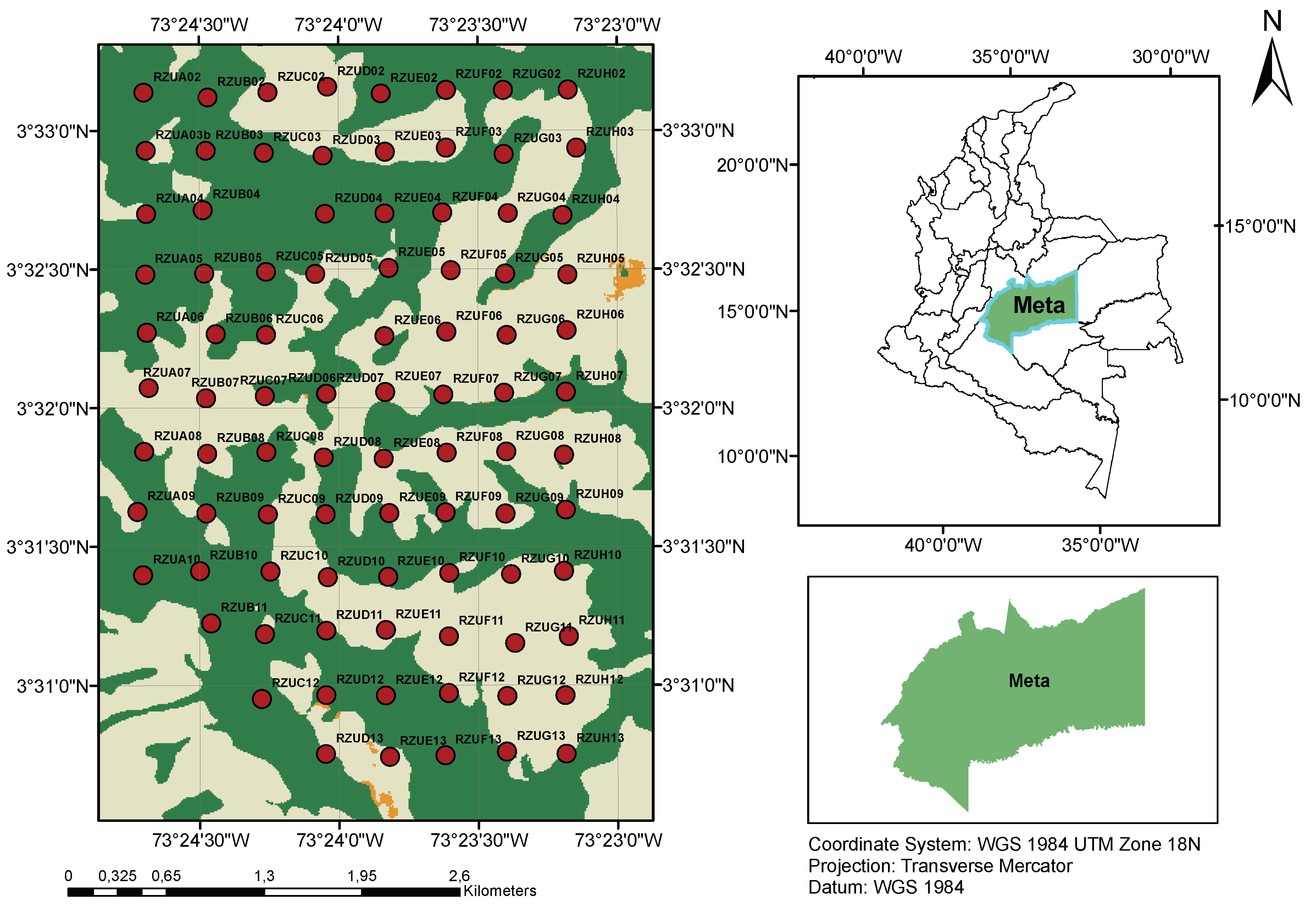
Figure 2.
Audio processing pipeline before feature extraction. The original audio recordings are downsampled from 192,000 Hz to 22,050 Hz. Each recording is then segmented into five 12-second segments. For each segment, a spectrogram is computed. Batches of these spectrograms are subsequently fed into the autoencoder network.
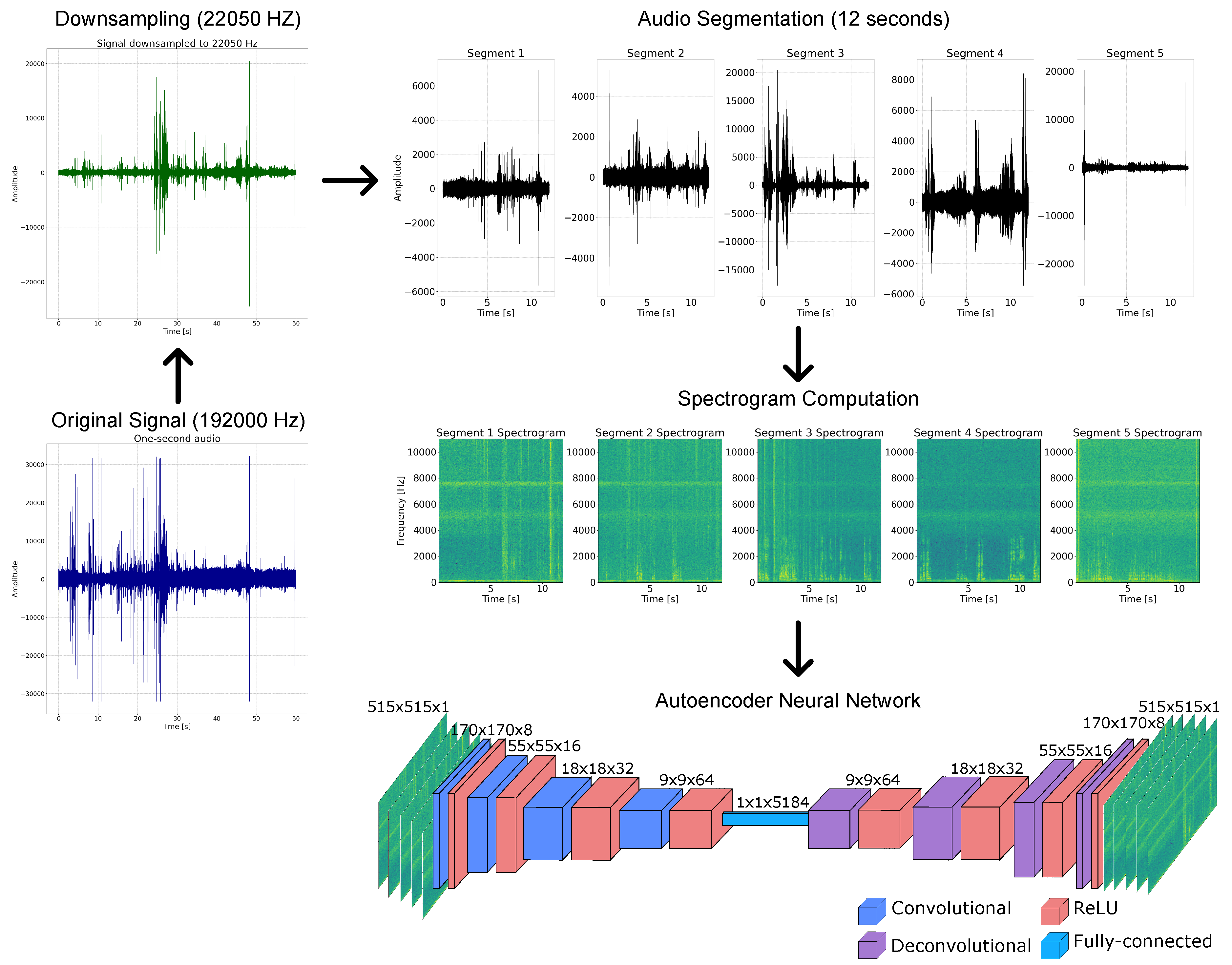
Figure 3.
Performance comparison of feature extraction methods on habitat classification across thirteen sampling days. The boxplots represent the distribution of (a) accuracy, (b) F1-score, and (c) recall obtained using Random Forest classifiers trained on features extracted by acoustic indices, VGGish, and autoencoder embeddings. The autoencoder consistently outperforms the other methods, demonstrating higher median scores and lower variability, indicating improved representational quality and robustness.
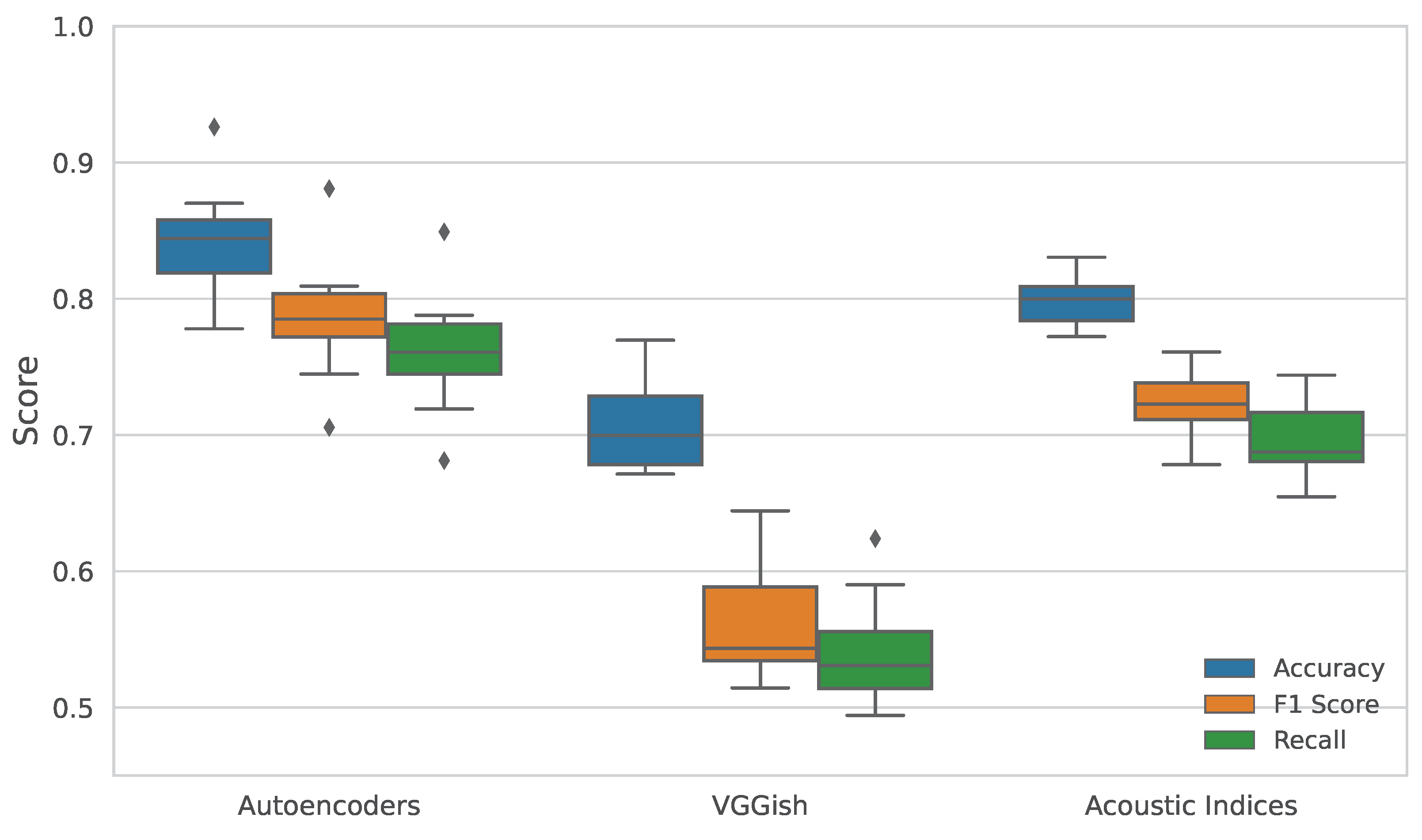
Figure 4.
Performance comparison of feature extraction methods on time-of-day classification across thirteen sampling days. The classification was performed using three temporal segments: dawn, midday, and dusk. The boxplots represent the distribution of (a) accuracy, (b) F1-score, and (c) recall obtained using Random Forest classifiers trained on features extracted by acoustic indices, VGGish, and autoencoder embeddings.
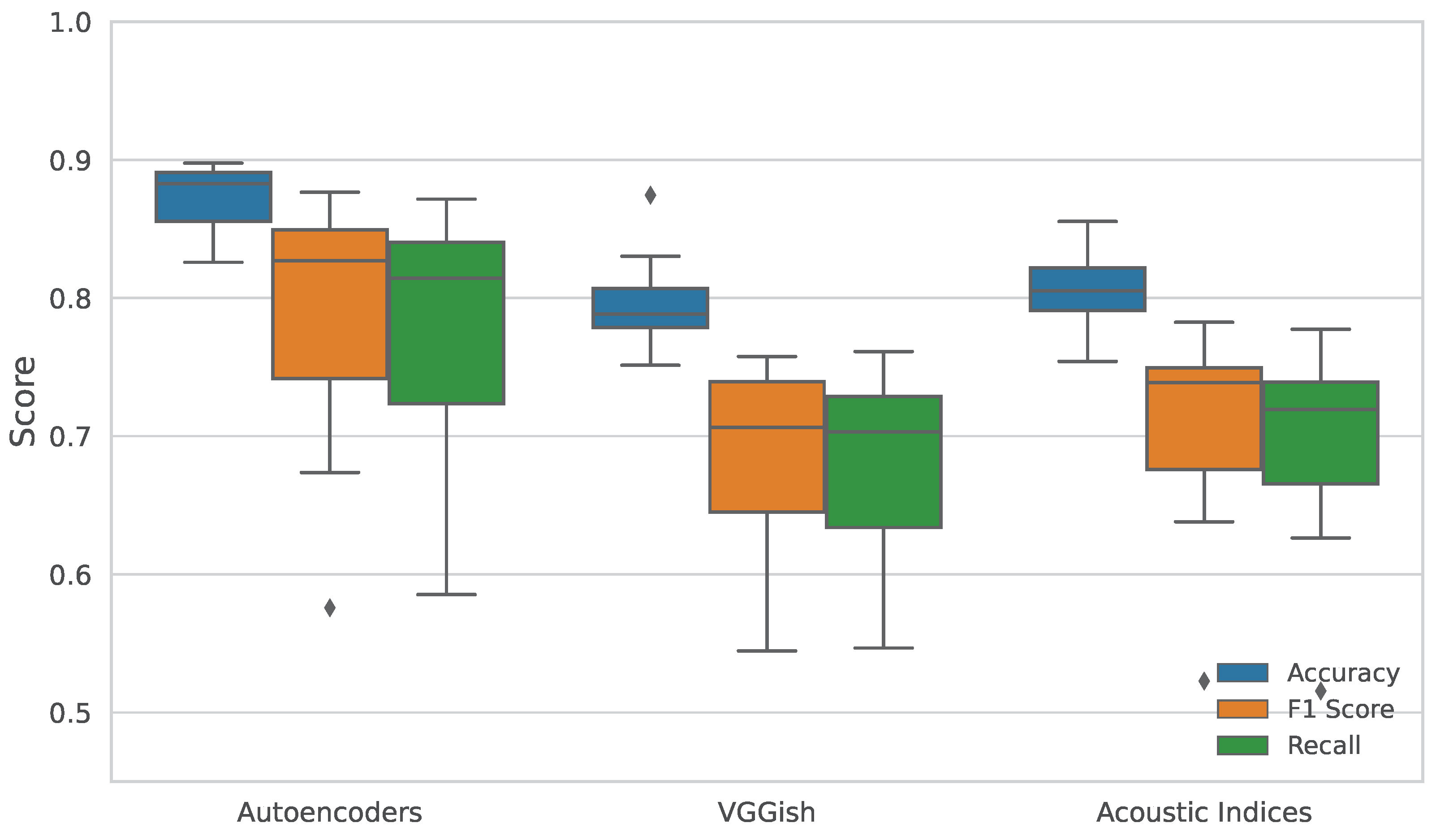
Figure 5.
Overview of the proposed unsupervised methodology. Feature extraction is performed using autoencoders, with acoustic indices included as a comparative baseline. The resulting embedding spaces are projected using PaCMAP and UMAP. These projections are then clustered by combining DBSCAN with PaCMAP and KMeans with UMAP. Finally, the evaluation scheme comprises three main components: spatial pattern analysis, comparative analysis using acoustic indices, and a novel connectivity approach based on acoustic similarity.
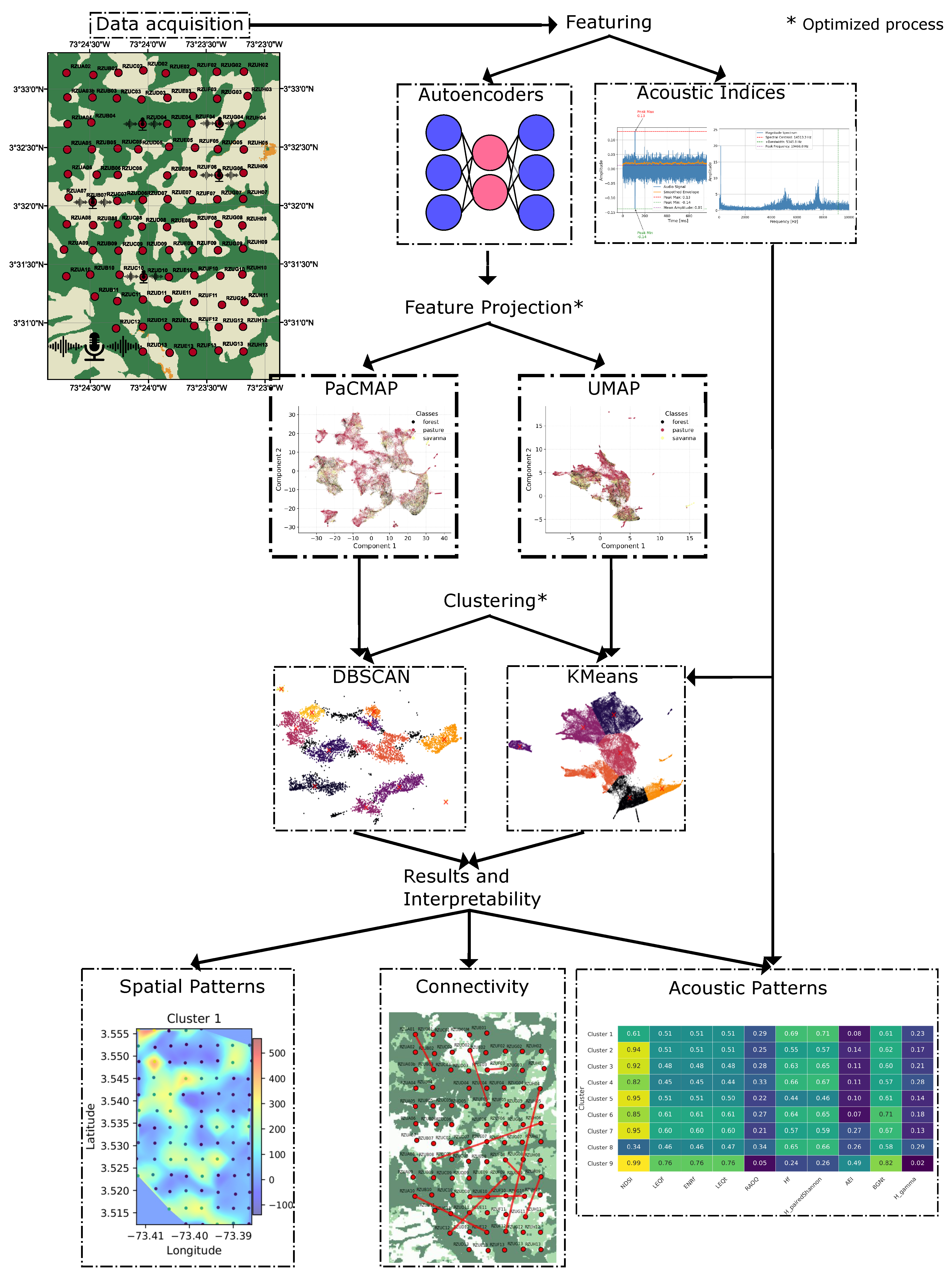
Figure 6.
Evaluation and visualization of low-dimensional embeddings generated by UMAP and PaCMAP. (a) Trustworthiness scores computed for a grid of parameter configurations in each method. The highest score for UMAP was achieved with 75 neighbors and a minimum distance of 0.01. For PaCMAP, the optimal configuration was 75 neighbors, a mid-scale neighbor ratio of 1.5, and a far neighbor ratio of 20. (b) Final low-dimensional projections of the dataset (subsampled), using the selected hyperparameters.
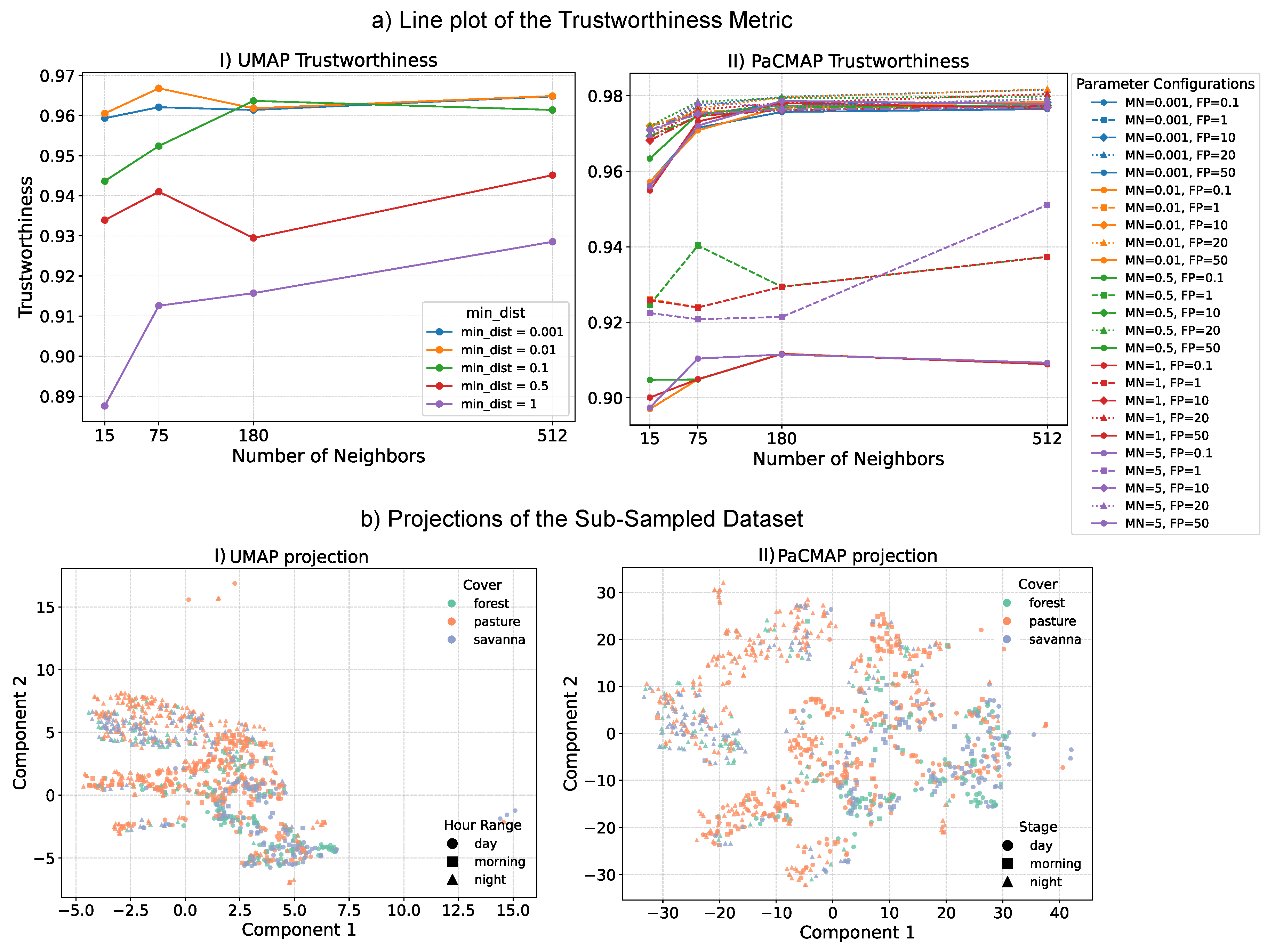
Figure 7.
Summary of KMeans clustering performance across different numbers of clusters using internal validation metrics. Each subplot shows a boxplot distribution of scores among days for a given number of clusters. (a) Silhouette Coefficient, where higher values indicate more cohesive and well-separated clusters; (b) Davies–Bouldin Index, where lower values indicate better clustering quality; and (c) Calinski–Harabasz Index, where higher values suggest better-defined cluster structure.
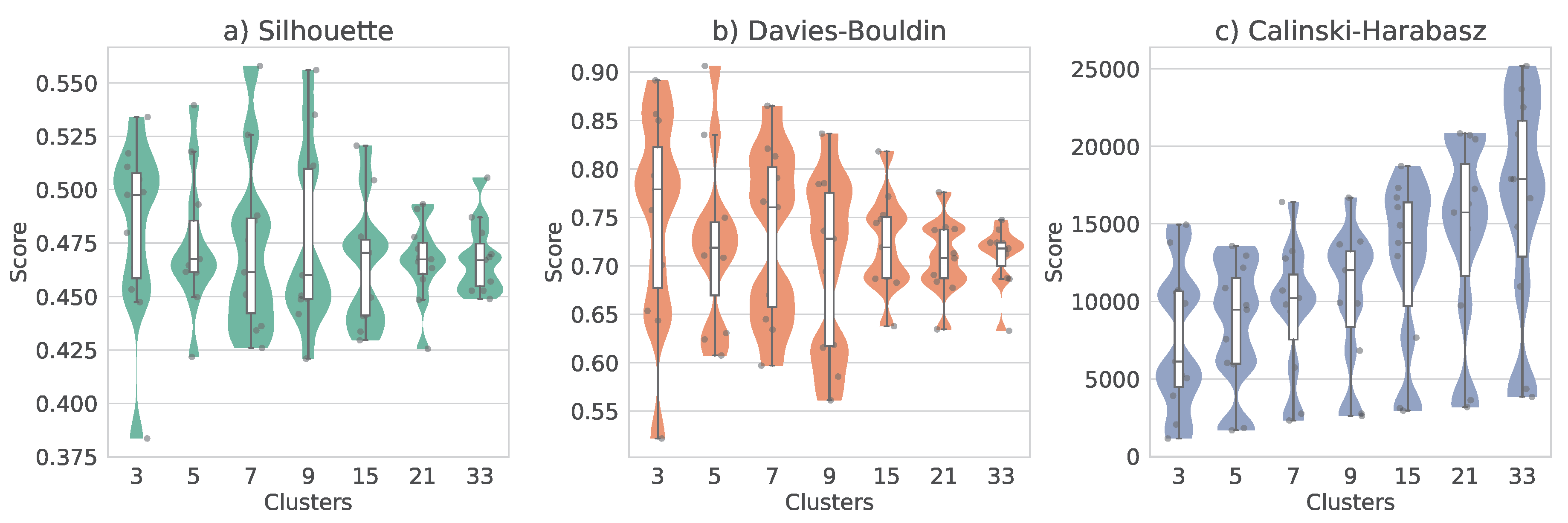
Figure 8.
Reachability plots for PaCMAP-embedded data across different sampling days.
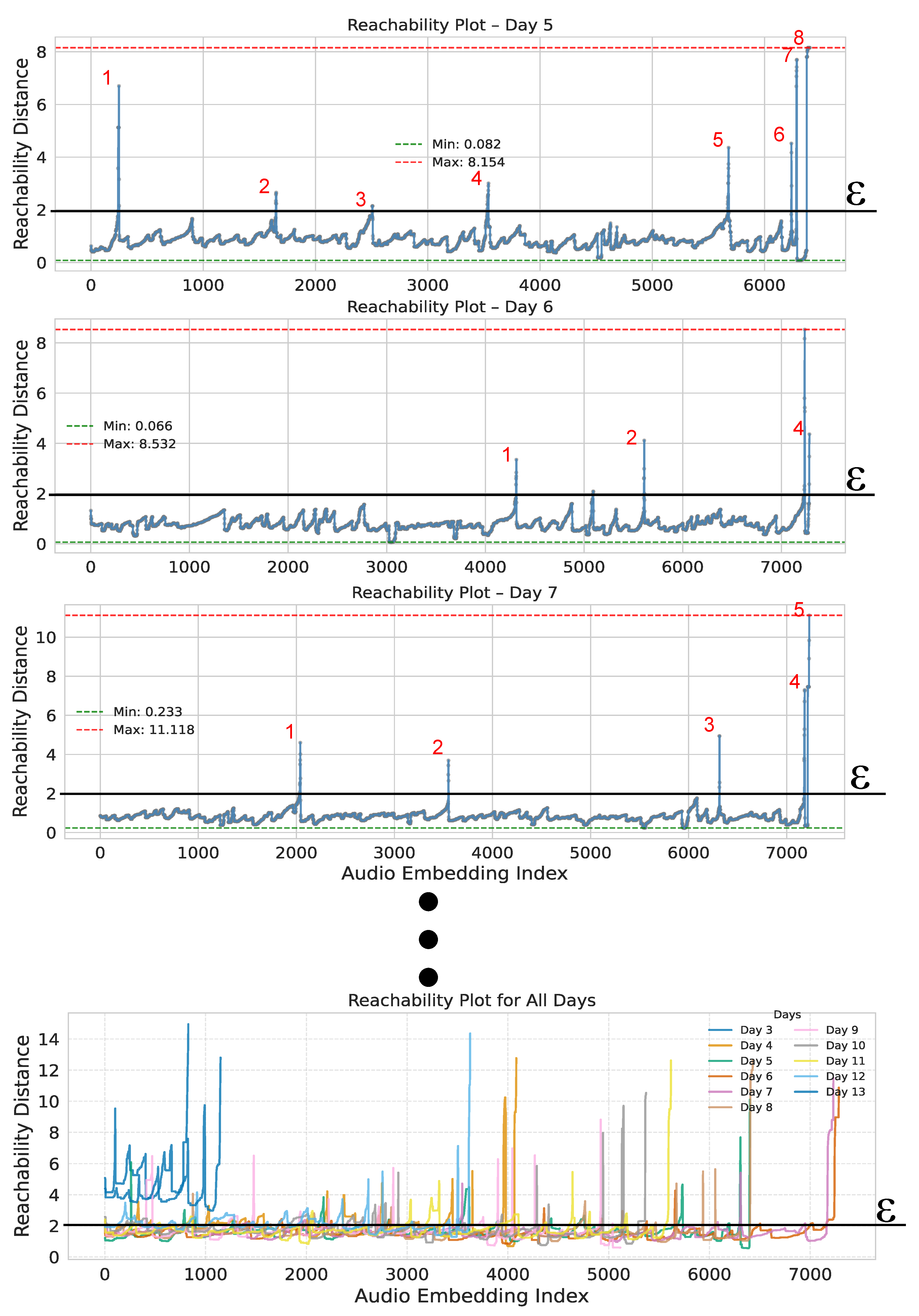
Figure 9.
Spatial distribution of acoustic clusters across the Zamuro Natural Reserve using PaCMAP projection and DBSCAN clustering. Each panel represents a heat map corresponding to one of the nine clusters. Color intensity indicates the relative number of audio samples associated with that cluster at each recording site.
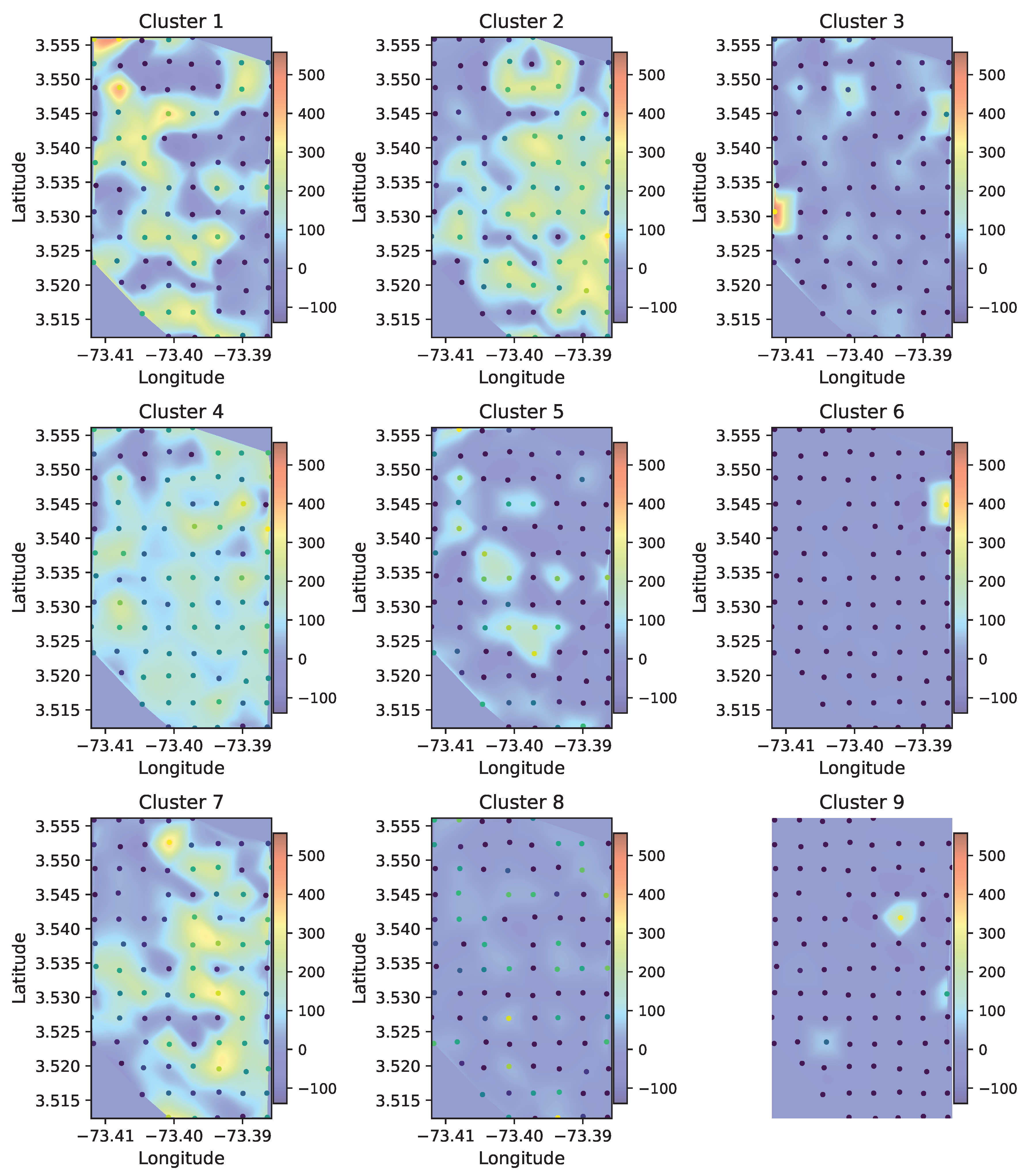
Figure 10.
Comparison of spatial distributions between the different clustering pipelines. Red boxes highlight areas where spatial overlap or similarity is observed between methods.
Figure 10.
Comparison of spatial distributions between the different clustering pipelines. Red boxes highlight areas where spatial overlap or similarity is observed between methods.
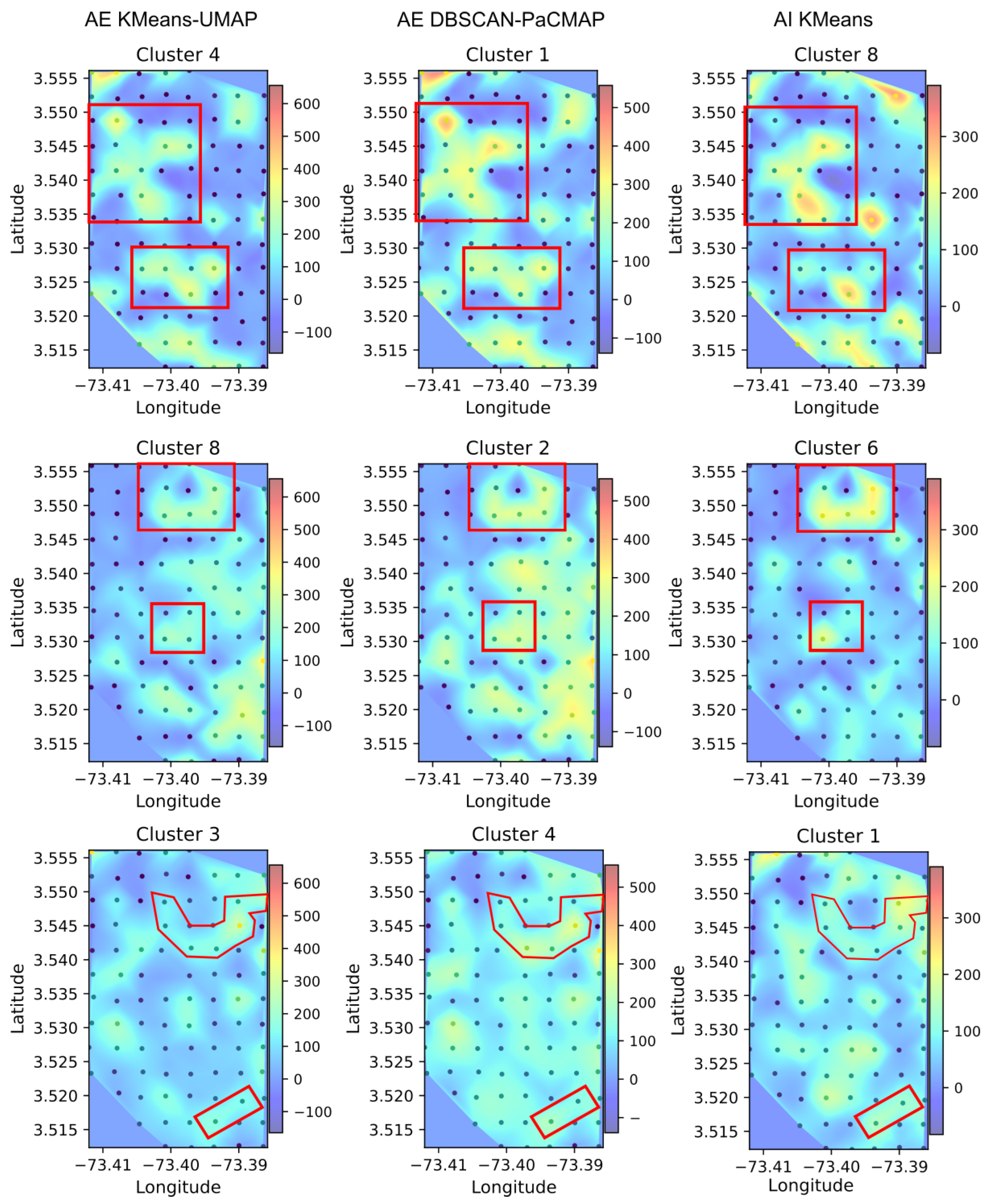
Figure 11.
Spatial distributions and decoded spectrograms for four selected clusters derived from UMAP projections and autoencoder embeddings. Each panel shows the heat map of cluster presence across the sampling grid (left) and the corresponding representative spectrogram reconstructed from the autoencoder latent space (right). This decoding enables the identification of dominant frequency bands associated with each cluster, facilitating the interpretation of their ecological and acoustic significance.
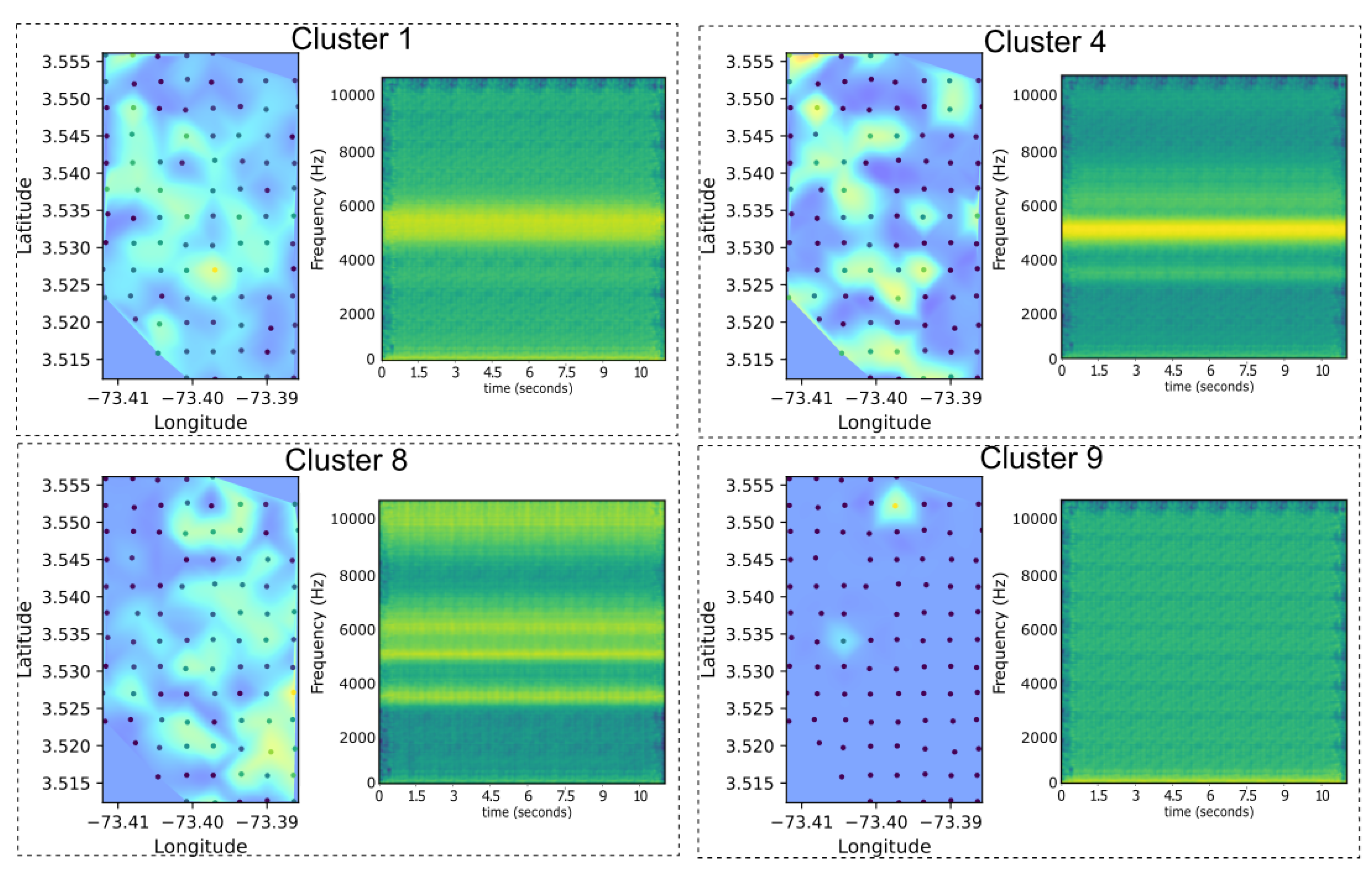
Figure 12.
Comparison of the acoustic indices with the highest inter cluster variance for both autoencoder based clustering (left) and baseline clustering using acoustic indices (right).
Figure 12.
Comparison of the acoustic indices with the highest inter cluster variance for both autoencoder based clustering (left) and baseline clustering using acoustic indices (right).
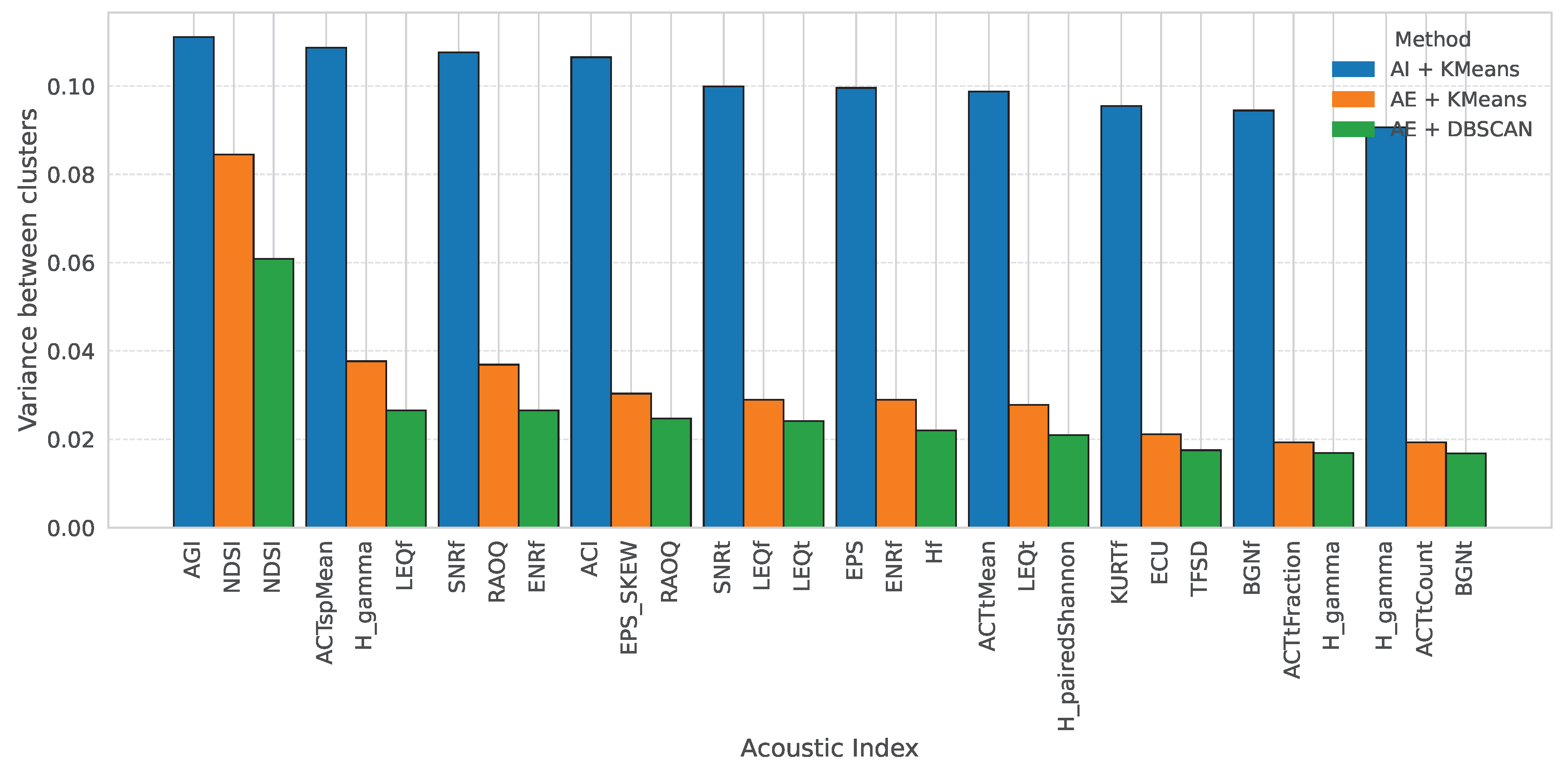
Figure 13.
Mean values of the top 10 acoustic indices per cluster for each analysis methodology.

Figure 14.
Examples of acoustic connectivity graphs for Days 4, 5, 6, and 7, constructed using PaCMAP projections and a threshold-based nearest neighbor approach.
Figure 14.
Examples of acoustic connectivity graphs for Days 4, 5, 6, and 7, constructed using PaCMAP projections and a threshold-based nearest neighbor approach.
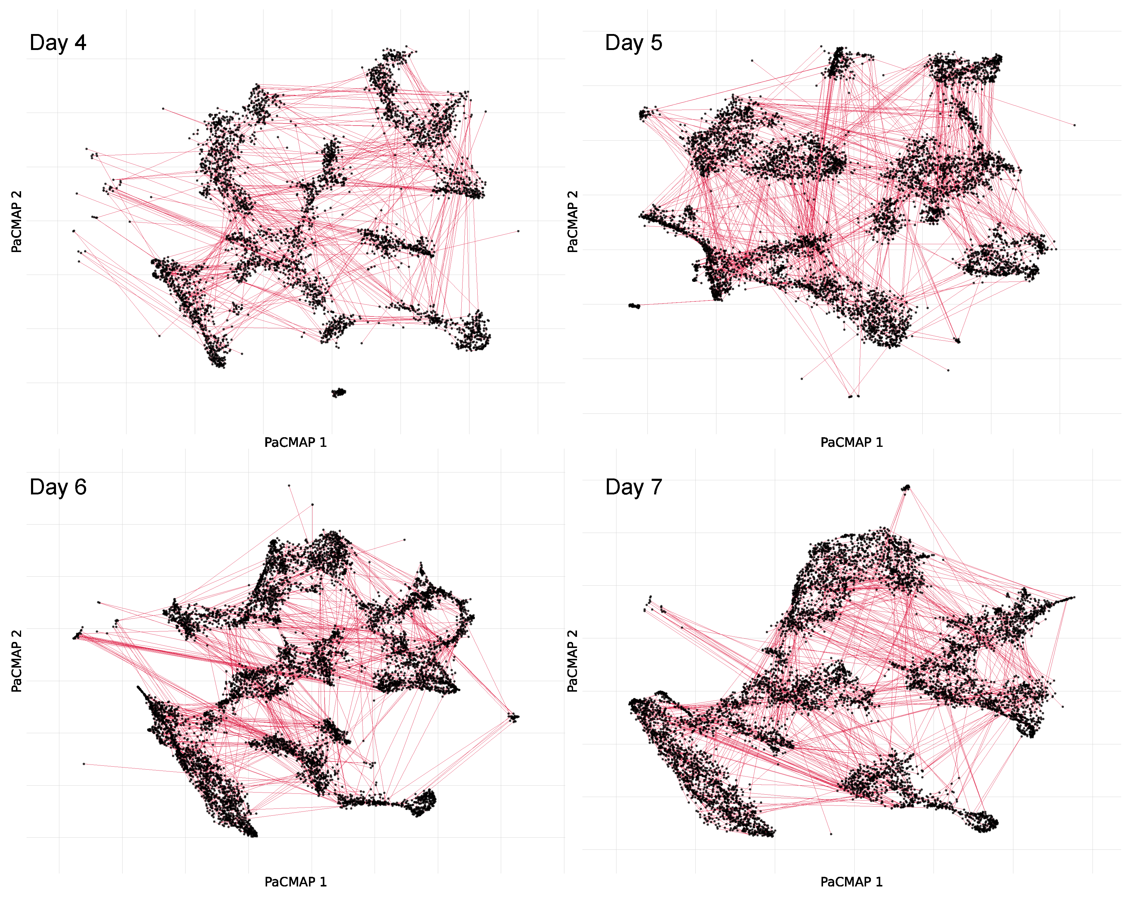
Figure 15.
Acoustic connectivity graph projected onto the physical layout of the Rey Zamuro reserve. Nodes represent recorder locations, and edges indicate acoustic similarity based on high-dimensional autoencoder embeddings. The background layer displays land cover types (forest, pasture, and savanna), providing ecological context. While several connections occur between nearby sites with similar cover types, long-range links are also present, revealing spatial acoustic patterns that extend beyond geographic proximity. This graph-based approach complements interpolation methods by highlighting both local and distant acoustic relationships across the landscape.
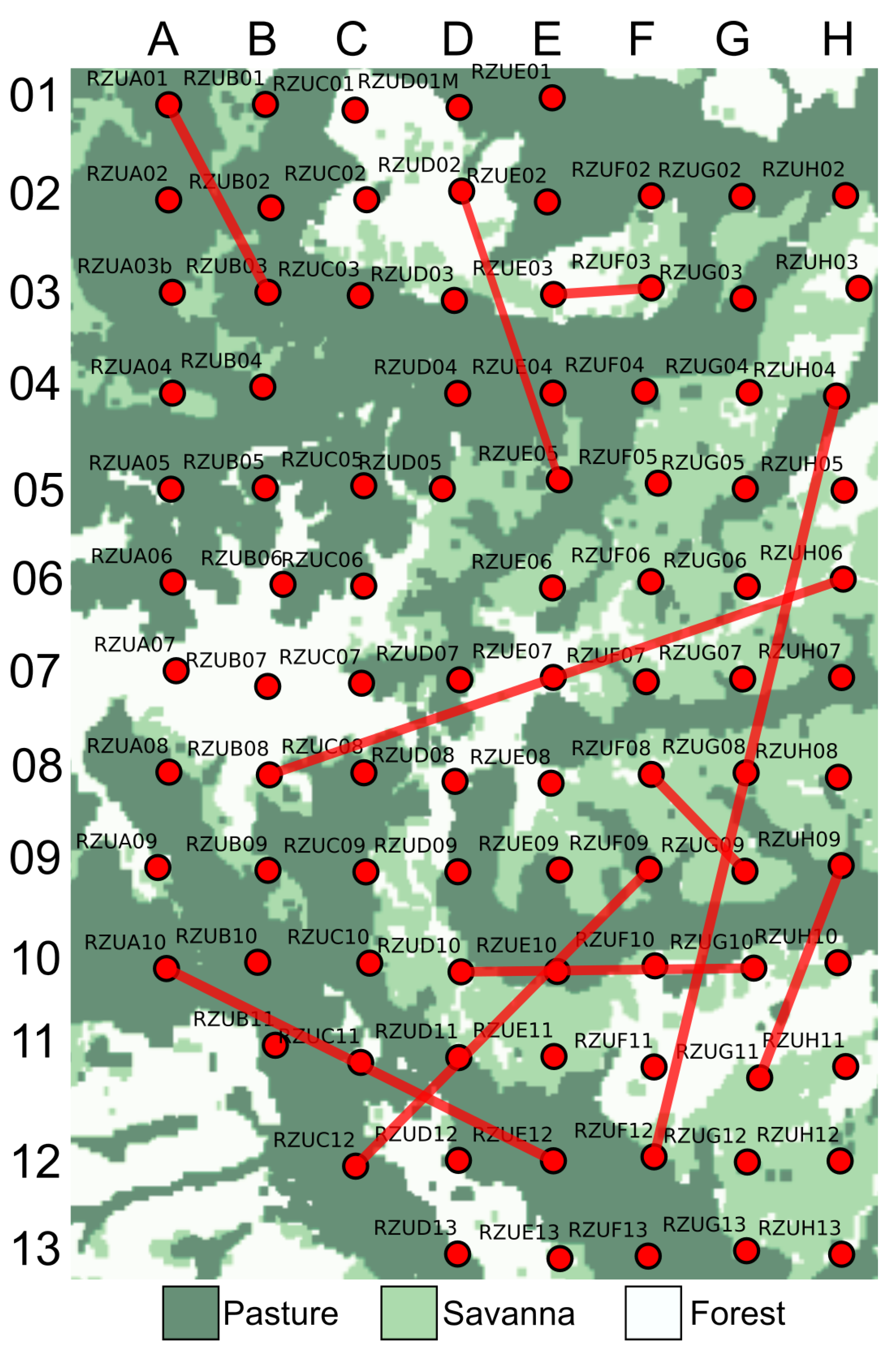
Table 1.
Statistical test results for performance metrics using cover types as labels in a multiclass classification approach. Significant p-values are marked as * (), ** (), and *** ().
Table 1.
Statistical test results for performance metrics using cover types as labels in a multiclass classification approach. Significant p-values are marked as * (), ** (), and *** ().
| Metric | Test | Comparison | Statistic | p-value |
|---|---|---|---|---|
| Accuracy | Friedman | AE, VGG, AI | 20.182 | 0.00004*** |
| Accuracy | Wilcoxon | AE vs VGG | 0.000 | 0.0010*** |
| Accuracy | Wilcoxon | AE vs AI | 1.000 | 0.0020** |
| Accuracy | Wilcoxon | VGG vs AI | 0.000 | 0.0010*** |
| F1 Score | Friedman | AE, VGG, AI | 20.182 | 0.00004*** |
| F1 Score | Wilcoxon | AE vs VGG | 0.000 | 0.0010*** |
| F1 Score | Wilcoxon | AE vs AI | 1.000 | 0.0020** |
| F1 Score | Wilcoxon | VGG vs AI | 0.000 | 0.0010*** |
| Recall | Friedman | AE, VGG, AI | 20.182 | 0.00004*** |
| Recall | Wilcoxon | AE vs VGG | 0.000 | 0.0010*** |
| Recall | Wilcoxon | AE vs AI | 1.000 | 0.0020** |
| Recall | Wilcoxon | VGG vs AI | 0.000 | 0.0010*** |
Table 2.
Statistical test results for performance metrics using three range of hours as labels. Significant p-values are marked as * (), ** (), and *** ().
Table 2.
Statistical test results for performance metrics using three range of hours as labels. Significant p-values are marked as * (), ** (), and *** ().
| Metric | Test | Comparison | Statistic | p-value |
|---|---|---|---|---|
| Accuracy | Friedman | AE, VGG, AI | 16.909 | 0.0002*** |
| Accuracy | Wilcoxon | AE vs VGG | 0.000 | 0.0010*** |
| Accuracy | Wilcoxon | AE vs AI | 0.000 | 0.0010*** |
| Accuracy | Wilcoxon | VGG vs AI | 20.000 | 0.2783 |
| F1 Score | Friedman | AE, VGG, AI | 15.273 | 0.0005*** |
| F1 Score | Wilcoxon | AE vs VGG | 0.000 | 0.0010*** |
| F1 Score | Wilcoxon | AE vs AI | 1.000 | 0.0020** |
| F1 Score | Wilcoxon | VGG vs AI | 13.000 | 0.0830 |
| Recall | Friedman | AE, VGG, AI | 14.364 | 0.0008*** |
| Recall | Wilcoxon | AE vs VGG | 0.000 | 0.0010*** |
| Recall | Wilcoxon | AE vs AI | 1.000 | 0.0020** |
| Recall | Wilcoxon | VGG vs AI | 18.000 | 0.2061 |
Disclaimer/Publisher’s Note: The statements, opinions and data contained in all publications are solely those of the individual author(s) and contributor(s) and not of MDPI and/or the editor(s). MDPI and/or the editor(s) disclaim responsibility for any injury to people or property resulting from any ideas, methods, instructions or products referred to in the content. |
© 2025 by the authors. Licensee MDPI, Basel, Switzerland. This article is an open access article distributed under the terms and conditions of the Creative Commons Attribution (CC BY) license (http://creativecommons.org/licenses/by/4.0/).
Copyright: This open access article is published under a Creative Commons CC BY 4.0 license, which permit the free download, distribution, and reuse, provided that the author and preprint are cited in any reuse.


