Submitted:
09 August 2025
Posted:
12 August 2025
You are already at the latest version
Abstract
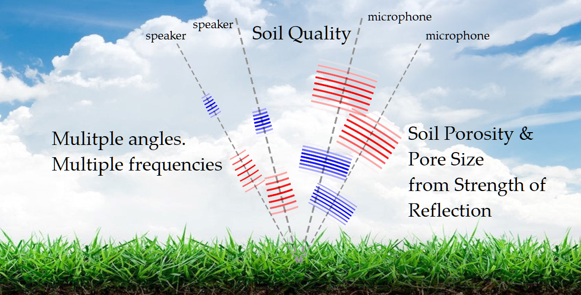
The purpose of this study is to investigate the potential for estimation of soil porosity and pore size (key indicators of soil physical health) using the strength of reflection of audio pulses from natural soil surfaces. The motivation for this work is the importance of productive and healthy soils in agriculture and other economic uses of land depending on plant growth. Soil porosity and pore structure are also significant in a wide range of environmental impacts such surface water runoff, and greenhouse gas exchanges.
Methods exist for evaluating soil porosity in a laboratory environment or by inserting sensors into the soil in the field. However, no convenient non-contact in situ measurement method exists. This means that existing soil evaluations do not generally sample adequately in either space or time. In the current study we develop a new methodology based on reflection of audio pulses in the frequency range 4 to 16 kHz. Such pulses are readily generated by, and analyzed with, for example, a mobile phone. The key to this very new method is a Taylor series expansion of the functional form of the acoustic reflectivity in a way that includes, embedded as simple linear regression coefficients, in a way which allows three soil parameters (porosity, tortuosity, and average pore radius) to be easily estimated. The requirements to set up these regressions are to generate pulses at a number of audio frequencies and a number of angles of incidence to the ground surface.
More than 3 million Monte Carlo simulations are performed using known random noise levels from the proposed sensor system. The simulation results show that both the systematic and random errors in estimation are very small, being typically less than 1 % for all three soil parameters. All assumptions and sources of error related to this method are discussed (to the best of the authors’ knowledge) and it is concluded that a practical new operational tool should be able to be readily manufactured and validated. This tool will be inexpensive, compact, low-power, non-intrusive to either the soil or the surrounding environment and will readily be incorporated into mobile phones as a fast and accurate means of visualizing farm-scale soil health.
Keywords:
soil physics
; precision agriculture
; soil quality
; non-contact acoustic sensing of soil properties
1. Introduction
Soil is the connection between the atmosphere and ground water, root systems, and sub-soil biological and chemical processes. Central to this connection is the degree to which air and water can penetrate the soil. This is primarily measured by the soil porosity, 𝜙, which is the ratio of the volume of spaces between soil particles to the total volume of a soil sample. Soil porosity significantly affects many important soil functions such as water, and air transmission, as well as water storage and availability to crops and pasture [1]. These soil functions in turn determine movement of nutrients and contaminants to water bodies, crops and pasture growth, and greenhouse gas emission [2]. Soil compaction, caused by activities like machinery use or animal traffic, reduces soil porosity by reducing the size and number of pore spaces [3]. Compacted soils have lower infiltration rates, poor drainage, and limited root penetration, leading to decreased plant productivity [4].
The spaces, or pores, between soil particles are not simple cylinders, leading to further soil physical parameters tortuosity, α∞ (the length of a pore following its path, divided by the shortest distance between the two ends of the pore), and the pore radius rpore. In practice there will be a wide range of pore geometries but, to first order, a single tortuosity and characteristic pore radius can be assigned to a soil sample.
Soil porosity is known to vary strongly and unpredictably in space and time as a result of management, such as the timing of tillage, crop management, and grazing practices [3,5]. Traditional methods for measuring soil porosity include: measuring the extra mass of water which is required to saturate a soil sample; use of a pycnometer to measure the air volume in the pore space for a soil sample in a gas-tight chamber; and compression of a soil sample to estimate the solid volume of soil [6]. Such methods require significant investments in time and labour [7]. Moreover, these existing methods provide fragmentary information in time and space and offer a limited capacity to assess temporal and spatial variation in soil health. In contrast, proximal sensing technologies have the potential to generate vastly more data at lower cost, providing that the complexity of such technologies do not present a barrier to adoption by land managers such as farmers.
Currently, soil pore size and pore connectivity measurement methods also rely on invasive methods [8]. For example, details of pore connectivity can be measured via X-ray imagery [9] but this requires specialised equipment in a laboratory environment. Nevertheless, pore size is a significant parameter in estimation of hydraulic flow [10].
Bradley et al. [11,12] developed a non-contact method for estimation of soil porosity and tortuosity based on the strength of reflections of ultrasound pulses. Their instrument could in principle be mounted on a farm vehicle, typically 1 m above the ground. At lower transmitted acoustic frequencies viscous interactions within the pores are dominant, whereas at high frequencies the dependence on air viscosity and on flow resistivity vanishes. These interactions of sound waves with the porous soil lead to a range of in-situ and laboratory methods which can be used to measure the morphological characteristics of porous materials [8]. Of these, only the reflection methods, which are applicable at high frequencies, lend themselves to proximal sensing. In this regime, the plane wave reflection coefficient depends only on angle of incidence, soil porosity, and soil tortuosity (a measure of the soil pore geometry), and not on the frequency of sound transmitted. By performing measurements at two or more angles of incidence, it is possible to estimate both porosity and tortuosity [13,14,15].
At low acoustic frequencies another parameter, the flow resistivity, can be estimated via reflection of sound [16]. The flow resistivity is related to the characteristic or average pore radius [8]. This suggests that a combination of ultrasound and low acoustic frequencies could yield estimates of porosity, tortuosity, and pore radius. However, the acoustic frequencies used for flow resistivity estimation are in the range 35– 75 Hz so that measurements are in the low-frequency viscous regime [16] and the propagation path was 50 m. This is problematic operationally for a proximal device operating at only 1 m from the target soil surface, given the wavelengths are in the range 4 – 10 m.
The purpose of the current work is to explore the potential of proximal sensing of soil pore radius in addition to porosity and tortuosity. This requires an extension of the previous work by Bradley et al. [11,12] to include frequency-dependence and, based on the above discussion, working with frequencies which are operationally practical. The goal is to develop a technology which can be applied at paddock or farm scale, based on a sensor mounted on a small farm vehicle.
2. Theory and Simulations
The aim is to estimate soil physical properties by using sound reflected from the soil surface, without disturbing the soil. This potentially will allow rapid assessment of soil physical health from a farm vehicle or drone. The proposed operational setup is shown schematically in Figure 1. A sound pulse of frequency f is incident on the soil surface at an angle of incidence θ from a directional speaker, and the reflected sound measured in the specular direction by a directional microphone. The ratio of the reflected pulse and the transmitted pulse is the plane wave reflection coefficient R. Some sound is transmitted into the soil so the amplitude |R| ≤ 1. In general, there is also a phase change upon reflection, including absorption.
2.1. Approximations for the Plane Wave Reflection Coefficient R
𝜙 is the soil porosity, ρe is an equivalent soil density and Ke the effective bulk density (allowing for the soil porosity), Ka is the bulk modulus of air, and ρ0 the air density.
The critical frequency fc is given by
where η is the dynamic viscosity of air and rpore is the characteristic (or mean) pore radius [6,8]. Note that, when the focus of research is on acoustics, the flow resistivity is generally used instead of rpore. The result of these approximations is
where
and
For Ω >> 1
where
This approximation was successfully used by Bradley and Ghimire [11] and Bradley et al. [12] to estimate soil porosity 𝜙 and soil tortuosity α∞ using the slope and intercept of a linear regression from measurements |R| at several angles of incidence θ and at an ultrasonic frequency of 25 kHz (see also [13,14,15]).
For Ω << 1
This was the asymptotic solution used by Sebaa et al. [16] for which Ω was in the range 0.035 to 0.075. Equation (14) suggests that, once 𝜙 and α∞ have been estimated from transmissions such that Ω >> 1 using Equation (12), a linear regression involving measurements at several transmissions such that Ω << 1 will allow an estimation of Ω and hence rpore.
2.2. Typical Values of Model Parameters
The strategy outlined above requires use of well-separated lower acoustic frequencies, flow, and higher acoustic frequencies, fhigh, satisfying
Table 1 gives typical values of parameters appearing in the above theory. Being simply a fraction of total volume, 𝜙 can range between 0 and 1, typically falling between 0.35 and 0.7 for soils [6]. Typical values for grasslands quoted by Salomons [18] are α∞ = 1.35, 𝜙 = 0.3, and 5 ≤ Ω ≤ 20 when the sound has a frequency of 25 kHz, equating to rpore = 63 – 125 μm.
The limitation on the angle of incidence arises from keeping the instrumentation reasonably compact. The limitations on transmitted frequency arise from aiming for directionality whilst not being too sensitive to scattering of sound by vegetation and surface roughness at higher frequencies. For a propagation path from speaker to ground to microphone of length L = 2 m (which would be a typical range from a small agricultural vehicle) and for an angle of incidence θ = 30°, the time for sound to travel horizontally between speaker and microphone is L/(2c0) = 3 ms if the sound speed c0 = 340 m s-1 (see Fig. 1). The time of first arrival of reflected sound is L/c0 = 6 ms. This means the duration of the acoustic pulse should be less than 3 ms. There are 12 cycles of 4 kHz sound in a 3 ms pulse, which would give a reasonable pulse shape for detection and peak analysis. For these parameters, one measurement would take L/c0 + L/(2c0) = 9 ms, so that around 100 measurements per second would be feasible if transmissions at all frequencies and angles of incidence simultaneous. However, an acoustic frequency of 4 kHz is considerably higher than the lowest likely critical frequency of 0.5 kHz. Similarly, the high acoustic frequency of 25 kHz is not much higher than the highest likely critical frequency of 22 kHz.
For example, assuming estimates of tortuosity and porosity have been made at higher frequencies, Figure 2 shows significant errors in estimated pore radius if Equation (14) is used with transmitted acoustic frequencies in the range of 1 – 5 kHz. There would also be concerns about external acoustic noise from, for example, engines, at these lower acoustic frequencies.
2.3. Approximation at Higher Frequencies
An alternative is to use higher acoustic frequencies and allow for the frequency-dependence of Y, where
Figure 3 shows the variation of Y with f for frequencies in the range 4 to 16 kHz. Also shown are the Y values at 1/3-octave frequencies in this band. The asymptotic high-frequency limit of these curves should give A and B and hence porosity 𝜙 and tortuosity α∞, and the curvature should give an estimate of Ω and hence fc and rpore.
The curvature can be found from a Taylor series expansion of the right-hand side of (7) in terms of Ω -1, Ω -2, ..., followed by expanding R from (7) as a series in in terms of Ω -1, Ω -2, ..., then expanding |R|, and finally Y from (16). This expansion is non-trivial. The result is
where
2.4. Procedure for Estimation of Soil Physical Parameters
We measure at an angle of incidence θm and at a transmitted frequency fn, where m = 1, 2, …, M and n = 1, 2,…, N.
For each θm perform a regression of Y vs f -2 as in (17), and using (5), to find estimates and of the coefficients, m = 1, 2, …, M, where
There are further expansion terms in (17) and (19) and, in order that κ or bm are representative of the first expansion term, we perform a polynomial fit of order 4. Given there are N = 7 frequencies, there is still sufficient redundancy in the regression. Using the M estimated values of and the M known values Xm do a single linear regression of a vs X
and from the two coefficients and estimate
It is now possible to estimate from (18), and
Hence estimate the characteristic pore radius
Note that M estimates are made of the pore radius, which are simply averaged.
3. Results
As an example, θm = 0°, 10°, 20°, and 30° for m = 1, 2, 3, 4 (M = 4), and fn = 4.00, 5.04, 6.35, 8.00, 10.08, 12.7, and 16.00 kHz for n = 1, 2, 3, 4, 5, 6, 7 (N = 7), giving MN = 28 measurements . The acoustic frequencies are in 1/3 octave steps. Values of with this set of θ and f values are given in Table 2, for porosity = 0.6, tortuosity = 1.6, and pore radius = 80 μm.
Simulations are performed for 5 soil porosity values of 0.4, 0.5, 0.6, 0.7, and 0.8, 5 tortuosity values of 1.4, 1.5, 1.6, 1.7, and 1.8, and 130 pore radius values from 50 μm to 179 μm in 1 μm steps. Values of are calculated for these 3250 simulated soil profiles, and for the M angles of incidence and N frequencies. Random gaussian noise εg with g = 1, 2, ….G, and having zero mean and standard deviation σR is added to each simulated
where ε is a random gaussian number of zero mean and standard deviation σR. With G = 1000 there are 3.2 x 10⁶ simulated reflectivity measurements. A value σR = 0.01 (1% variability in measured |R|) was used, consistent with actual measurements [11].
For each soil “profile”, or group of simulation 𝜙, α∞, and rpore values, estimates , , and are made from the G noisy “measurements”. Mean values and standard deviations of estimates are found for each of the 3250 simulated soil profiles.
There are two main sources of error: model error and random measurement noise error (systematic measurement errors can be made negligible with good hardware design and calibration). Model error manifests as bias in estimates, whereas noise error manifests as both bias and random fluctuations in estimates. Bias β is estimated from
and random uncertainty s from
and similarly for tortuosity and pore radius. Values of these measures averaged across all soil profiles are shown in Table 3.
The parameter estimation errors shown in Table 3 give no indication of whether more accurate estimates might be obtained from certain combinations of soil parameters. In order to answer this, β and s are averaged over 2 of the 3 soil parameters giving, for example, β𝜙, ∞(rpore) for β averaged over all 𝜙 and α∞ as a function of rpore . The results are plotted in Figure 4 and Figure 5. It is clear that the bias and random errors are low (a few %) and largely independent of soil properties except for a strong dependence on lower rpore values. These 3 (solid line) bias curves reach 2% for rpore smaller than about 60 μm. Estimates of all three soil parameters have significant errors for low pore size. Bias errors are also simulated with zero random noise, giving a very similar plot to Figure 4. This indicates that the bias errors are almost entirely due to model errors. Since these errors are systematic, they could be corrected by fitting curves to the error curves, although we have not attempted that here since the errors are very small.
Random fluctuation errors only appear if σR > 0. Tortuosity estimates are sensitive to low pore radius, reaching around 1.5% fluctuation errors for rpore = 50 μm. Random errors of this magnitude are acceptable.
4. Discussion
The approach taken here to estimate soil physical properties is very different from traditional laboratory-based methods. Our method allows fast non-contact in situ simultaneous estimates of soil porosity, tortuosity and soil pore radius. This method also differs dramatically from the asymptotic acoustic methods used by others in either a very high-frequency domain or a very low-frequency domain. The key new element is the expansion of the full expression for the plan wave reflection coefficient R in a Taylor series with terms in 1/Ω 2, 1/Ω 4,… Only the coefficient of the first expansion term (in 1/Ω 2) has been developed, yielding an expression for the pore radius. A further linear regression is required to obtain estimates of porosity and tortuosity from the same set of measurements.
A Monte Carlo simulation shows that the primary source of uncertainty in soil parameter estimation is model error. These errors are very small, being typically less than 1 %, and arise from truncation of the Taylor series expansion to 4 terms (proportional to 1, 1/Ω 2, 1/Ω 4, and 1/Ω 6). The expansion is truncated so that the polynomial regression is over-determined with 7 acoustic frequencies and the 4 expansion coefficients.
In practice this analysis compares one model (the Taylor series approach) with another which assumes (1) – (6) are valid. The robustness of this approach therefore depends on
- Accuracy of (6). Horoshenkov [8] used this relationship to estimate the radius of glass beads based on known packing, obtaining agreement to within 9%. This is equivalent to a 9% standard deviation in estimated pore radius.
- The assumed value σR = 0.01 for the Monte Carlo simulations. Bradley et al. [12] show an example of a received pulse in which the rms amplitude noise is around 3 mV on a signal of amplitude 80 mV. A group of 16 such pulses are used to fit a known pulse shape to the data. If the pulse peak is used, without any pulse shape fitting, the relative standard deviation is σR = (3/80)/4 or 0.9%. In practice fitting a known shape to the pulse data will give a smaller uncertainty in |R|. Uncertainties in estimated parameters simply scale with σR at these low levels.
- The assumption that errors due to signal loss in sound passing through grass and roughness are small. The relevant scattering parameter is 2πfh/c0 where f is the acoustic frequency and h is the dimension of a scattering object. For pasture swards h is of order 5 mm and 2πfh/c0 is around 1. At this value of the scattering parameter some loss of reflected energy will occur [24]. For soil particles forming a rough soil surface, the scattering parameter will generally be smaller [12]. For pugging due to animal hoof prints, major scattering can be expected. In all these cases the best operational strategy may be to detect scattering at each angle of incidence using the multiple microphones and, if scattered energy is more than a few percent of the incident energy, discard that data point [12].
These caveats do not appear to limit the scope and credibility of the new approach taken here. Of course, design of hardware and software generally also involves compromises, but previous work [11,24] gives confidence that a suitable design should be practical. This is particularly true given the availability of a much wider range of transmitting and receiving devices in the audio spectrum compared with the ultrasonic region. The new methodology also lends itself much more to being controlled entirely from a mobile phone because the audio interfaces on modern phones have the requisite bandwidth and sampling rates. The ultimate goal is therefore a compact rigid array of speakers and microphones which can be mounted on a small farm vehicle such as a quad-bike, with data recorded on a mobile phone and able to be readily uploaded to a farm management system.
Symbols
| Symbol | Description |
| a | A+BX |
| A | 𝜙2/α∞ |
| b | Coefficient of f -2 in expansion |
| B | A(α-1)/ α∞ |
| c | A(1+X) |
| c0 | Speed of sound |
| d | -AX/ α∞ |
| f | Acoustic frequency |
| fc | Critical frequency |
| flow | A frequency much lower than fc |
| fhigh | A frequency much higher than fc |
| G | Number of random realizations |
| Ka | Bulk modulus of air |
| Ke | Effective bulk density of soil |
| L | Acoustic path length for reflection |
| m | Index of θ |
| M | Maximum value of m |
| n | Index of f |
| N | Maximum value of n |
| rpore | Characteristic pore radius |
| R | Plane wave reflection coefficient |
| |R| | Amplitude of R |
| s | Relative standard deviation of estimates |
| X | tan2θ |
| Y | (1-|R|)2/(1+|R|)2 |
| α∞ | Soil tortuosity |
| β | Bias in estimates |
| γ | iΩ /(1+ iΩ) |
| /ε | Fractional random noise in measurement |R| |
| η | Dynamic viscosity of air |
| θ | Angle of incidence |
| κ | Curvature of Y vs Ω-2 |
| ρ0 | Air density |
| ρe | Equivalent soil density |
| σR | Standard deviation of noise in measurement |R| |
| 𝜙 | Soil porosity |
| Ω | Normalized frequency |
Author Contributions
This work was motivated by earlier work of Bradley and Ghimire on using ultrasonic reflections to estimate soil porosity and tortuosity. The authors recognized the need to also estimate soil pore structures. Conceptualization, Bradley and Ghimire; methodology, Bradley; software, Bradley; formal analysis, Bradley; investigation, Bradley; writing—original draft preparation, Bradley; writing—review and editing, Ghimire and Bradley; visualization, Bradley and Ghimire. All authors have read and agreed to the published version of the manuscript.
Funding
This research received no external funding.
Data Availability Statement
Data from the simulations are available in the manuscript.
Conflicts of Interest
The authors declare no conflicts of interest.
References
- Ngo-Cong, D.; Antille, D.L.; Th. van Genuchten, M.; Nguyen, H.Q.; Tekeste, M.Z.; Baillie, C.P.; Godwin, R.J. A Modeling Framework to Quantify the Effects of Compaction on Soil Water Retention and Infiltration. Soil Science Society of America Journal 2021, 85, 1931–1945. [Google Scholar] [CrossRef]
- Hu, W.; Drewry, J.; Beare, M.; Eger, A.; Müller, K. Compaction Induced Soil Structural Degradation Affects Productivity and Environmental Outcomes: A Review and New Zealand Case Study. Geoderma 2021, 395, 115035. [Google Scholar] [CrossRef]
- Drewry, J.J.; Cameron, K.C.; Buchan, G.D.; Drewry, J.J.; Cameron, K.C.; Buchan, G.D. Pasture Yield and Soil Physical Property Responses to Soil Compaction from Treading and Grazing — a Review. Soil Res. 2008, 46, 237–256. [Google Scholar] [CrossRef]
- Alaoui, A.; Rogger, M.; Peth, S.; Blöschl, G. Does Soil Compaction Increase Floods? A Review. Journal of Hydrology 2018, 557, 631–642. [Google Scholar] [CrossRef]
- Mateo-Marín, N.; Bosch-Serra, À.D.; Molina, M.G.; Poch, R.M. Impacts of Tillage and Nutrient Management on Soil Porosity Trends in Dryland Agriculture. European Journal of Soil Science 2022, 73, e13139. [Google Scholar] [CrossRef]
- Nimmo, J.R. Porosity and Pore Size Distribution. In Reference Module in Earth Systems and Environmental Sciences; Elsevier, 2013; p. B9780124095489052659 ISBN 978-0-12-409548-9.
- Ghajar, S.; Tracy, B. Proximal Sensing in Grasslands and Pastures. Agriculture 2021, 11, 740. [Google Scholar] [CrossRef]
- Horoshenkov, K.V. A Review of Acoustical Methods for Porous Material Characterisation. IJAV 2017, 22. [Google Scholar] [CrossRef]
- Lucas, M.; Vetterlein, D.; Vogel, H.-J.; Schlüter, S. Revealing Pore Connectivity across Scales and Resolutions with X-Ray CT. European Journal of Soil Science 2021, 72, 546–560. [Google Scholar] [CrossRef]
- Manns, H.R.; Jiang, Y.; Parkin, G. Soil Pores in Preferential Flow Terminology and Permeability Equations. Vadose Zone Journal 2024, 23, e20365. [Google Scholar] [CrossRef]
- Bradley, S.; Ghimire, C. Design of an Ultrasound Sensing System for Estimation of the Porosity of Agricultural Soils. Sensors 2024, 24, 2266. [Google Scholar] [CrossRef] [PubMed]
- Bradley, S.G.; Ghimire, C.; Taylor, A. Estimation of the Porosity of Agricultural Soils Using Non-Contact Ultrasound Sensing. Soil Advances 2024, 1, 100003. [Google Scholar] [CrossRef]
- Fellah, Z.E.A.; Berger, S.; Lauriks, W.; Depollier, C.; Fellah, M. Measuring the Porosity of Porous Materials Having a Rigid Frame via Reflected Waves: A Time Domain Analysis with Fractional Derivatives. Journal of Applied Physics 2003, 93, 296–303. [Google Scholar] [CrossRef]
- Fellah, Z.E.A.; Berger, S.; Lauriks, W.; Depollier, C.; Aristégui, C.; Chapelon, J.-Y. Measuring the Porosity and the Tortuosity of Porous Materials via Reflected Waves at Oblique Incidence. The Journal of the Acoustical Society of America 2003, 113, 2424–2433. [Google Scholar] [CrossRef] [PubMed]
- Fellah, Z.E.A.; Mitri, F.G.; Depollier, C.; Berger, S.; Lauriks, W.; Chapelon, J.Y. Characterization of Porous Materials with a Rigid Frame via Reflected Waves. J. Appl. Phys. 2003, 94, 7914. [Google Scholar] [CrossRef]
- Sebaa, N.; Fellah, Z.E.A.; Fellah, M.; Lauriks, W.; Depollier, C. Measuring Flow Resistivity of Porous Material via Acoustic Reflected Waves. Journal of Applied Physics 2005, 98. [Google Scholar] [CrossRef]
- Brennan, M.J.; To, W.M. Acoustic Properties of Rigid-Frame Porous Materials — an Engineering Perspective. Applied Acoustics 2001, 62, 793–811. [Google Scholar] [CrossRef]
- Salomons, E.M. Computational Atmospheric Acoustics; Springer Science & Business Media, 2001; ISBN 978-1-4020-0390-5.
- Allard, J.-F.; Atalla, N. Propagation of Sound in Porous Media: Modelling Sound Absorbing Materials; 2nd ed.; Wiley: Hoboken, N.J, 2009; ISBN 978-0-470-74661-5. [Google Scholar]
- Panneton, R. Comments on the Limp Frame Equivalent Fluid Model for Porous Media. The Journal of the Acoustical Society of America 2007, 122, EL217–EL222. [Google Scholar] [CrossRef] [PubMed]
- Fellah, Z.E.A.; Fellah, M.; Depollier, C.; Ogam, E.; Mitri, F.G. Ultrasound Measuring of Porosity in Porous Materials. In Porosity - Process, Technologies and Applications; Ghrib, T.H., Ed.; InTech, 2018 ISBN 978-1-78923-042-0.
- Lieblappen, R.; Fegyveresi, J.M.; Courville, Z.; Albert, D.G. Using Ultrasonic Waves to Determine the Microstructure of Snow. Front. Earth Sci. 2020, 8, 34. [Google Scholar] [CrossRef]
- Umnova, O.; Attenborough, K.; Shin, H.-C.; Cummings, A. Deduction of Tortuosity and Porosity from Acoustic Reflection and Transmission Measurements on Thick Samples of Rigid-Porous Materials. Applied Acoustics 2005, 66, 607–624. [Google Scholar] [CrossRef]
- Legg, M.; Bradley, S. Ultrasonic Proximal Sensing of Pasture Biomass. Remote Sensing 2019, 11, 2459. [Google Scholar] [CrossRef]
Figure 1.
The measurement configuration.
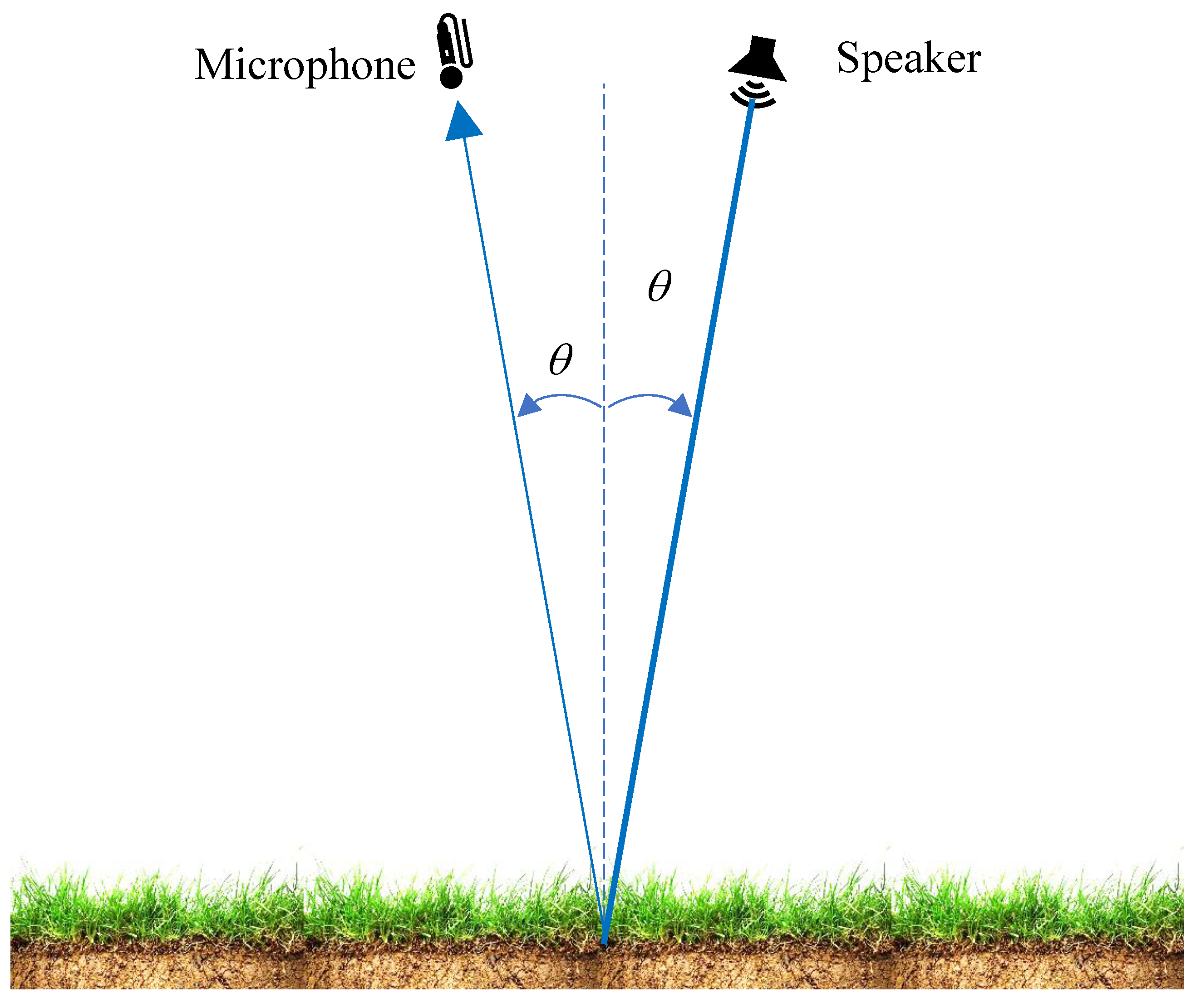
Figure 2.
Pore radius estimated from (14) compared with the true pore radius when f -> 0 (black), f = 1 kHz (red), f = 2 kHz (blue), f = 3 kHz (green), f = 4 kHz (magenta), and f = 5 kHz (yellow). The soil porosity is 0.6 and the tortuosity 1.4.
Figure 2.
Pore radius estimated from (14) compared with the true pore radius when f -> 0 (black), f = 1 kHz (red), f = 2 kHz (blue), f = 3 kHz (green), f = 4 kHz (magenta), and f = 5 kHz (yellow). The soil porosity is 0.6 and the tortuosity 1.4.
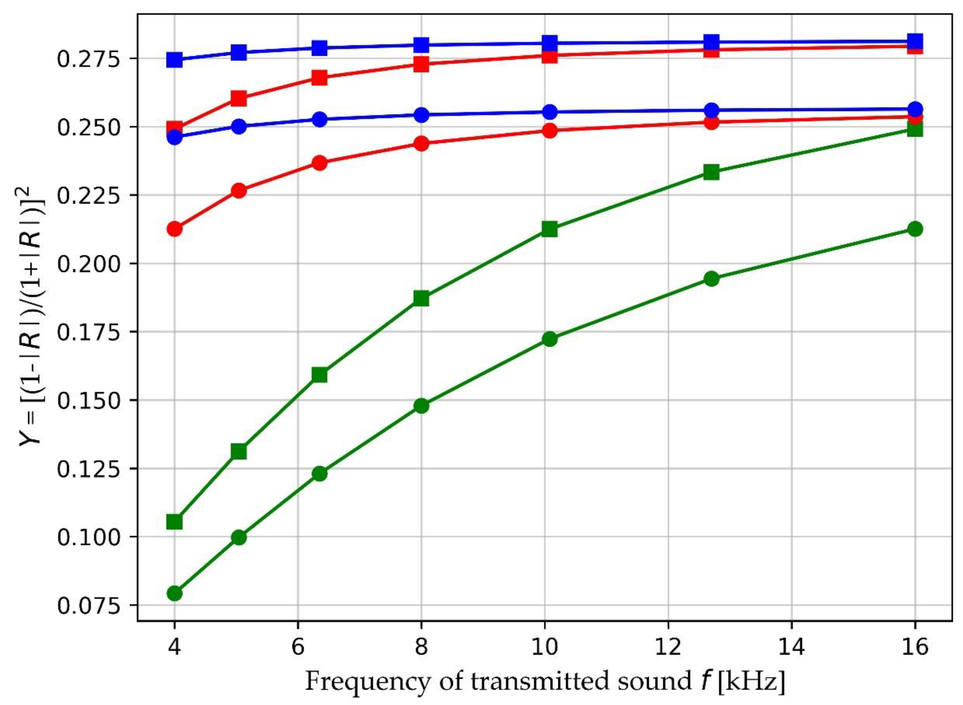
Figure 3.
The behaviour of Y at higher audio frequencies at θ = 0° (circles), θ = 30° (squares), and for rpore = 50 μm (green curves), 100 μm (red curves), and 150 μm (blue curves). The soil porosity is 0.6 and the tortuosity 1.4.
Figure 3.
The behaviour of Y at higher audio frequencies at θ = 0° (circles), θ = 30° (squares), and for rpore = 50 μm (green curves), 100 μm (red curves), and 150 μm (blue curves). The soil porosity is 0.6 and the tortuosity 1.4.
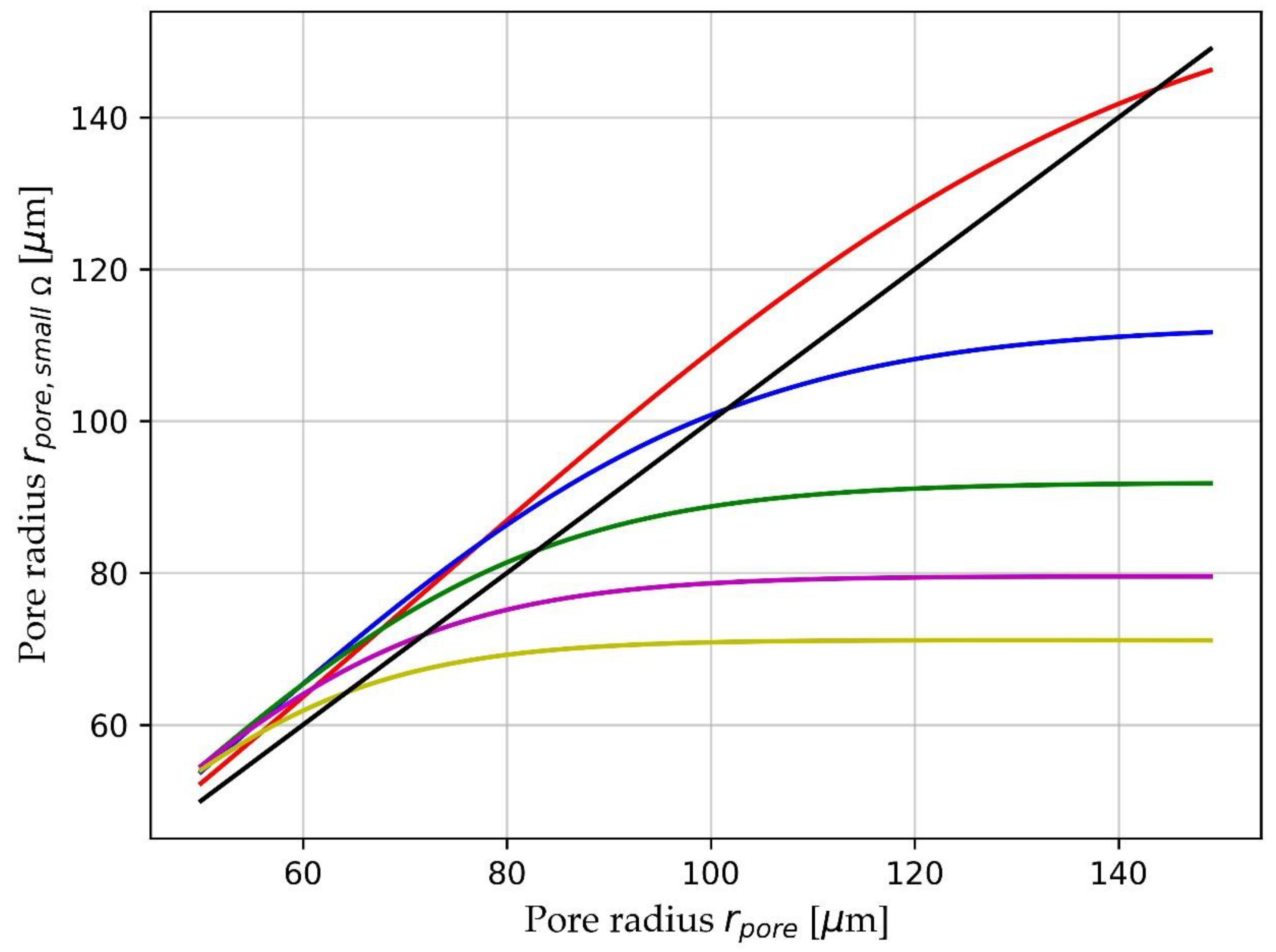
Figure 4.
The fractional bias β in estimated soil parameters porosity (red), tortuosity (blue) and soil pore radius (green). The fractional noise in |R| is σR = 0.01. Fractional bias errors are averaged over 2 of the 3 soil parameters and plotted against the 3rd parameter (𝜙 dotted lines, α∞ dashed lines, and rpore solid lines). The abscissa are values of the parameters scaled to their minimum value at an abscissa value 0.0 and their maximum value at an abscissa value of 1.0.
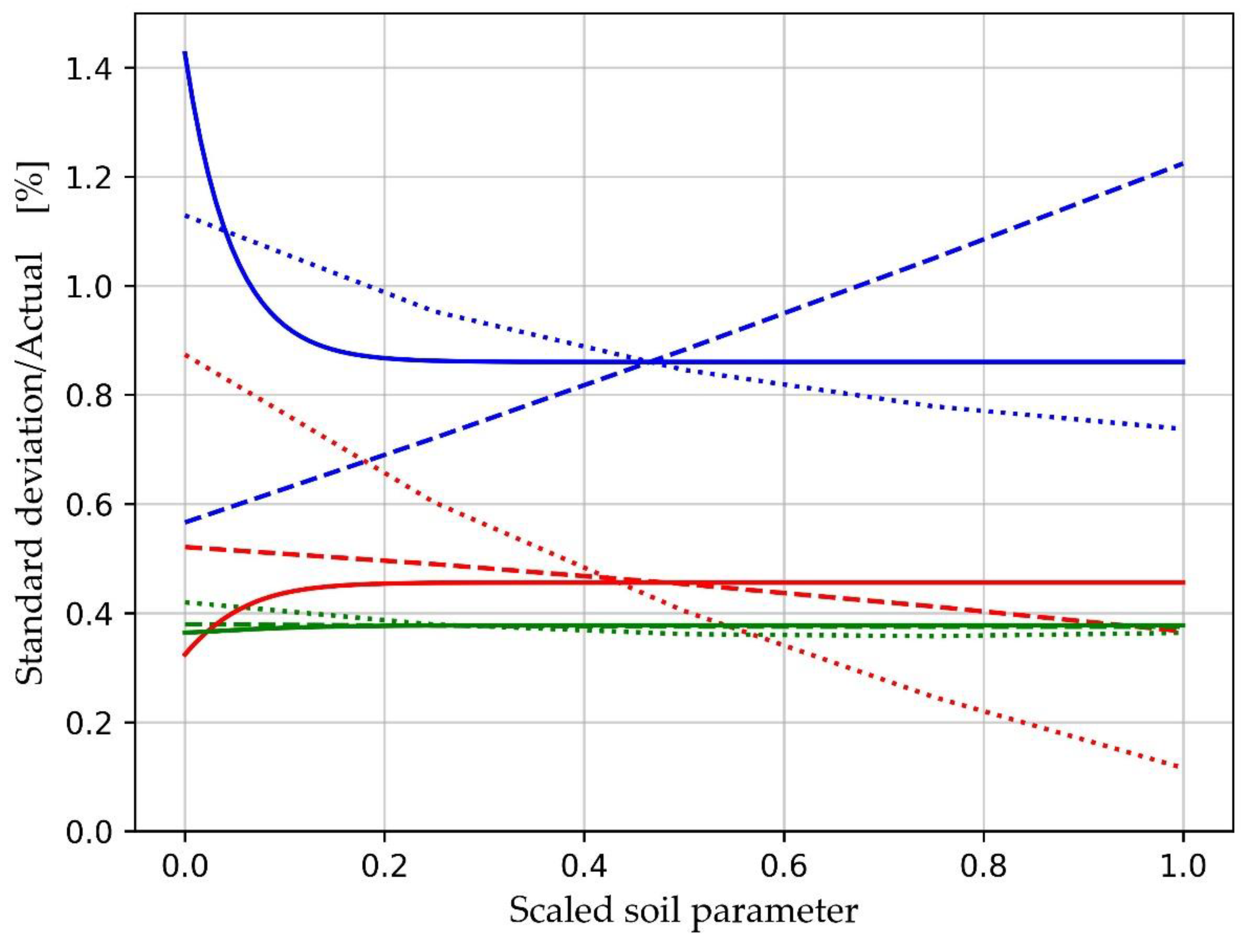
Figure 5.
The relative standard deviation in soil parameter estimation for porosity (red), tortuosity (blue), and soil pore radius (green). The fractional noise in |R| is σR = 0.01. Fractional errors are averaged over 2 of the 3 soil parameters and plotted against the 3rd parameter (𝜙 dotted lines, α∞ dashed lines, and rpore solid lines). The abscissa are values of the parameters scaled to their minimum value at an abscissa value 0.0 and their maximum value at an abscissa value of 1.0.
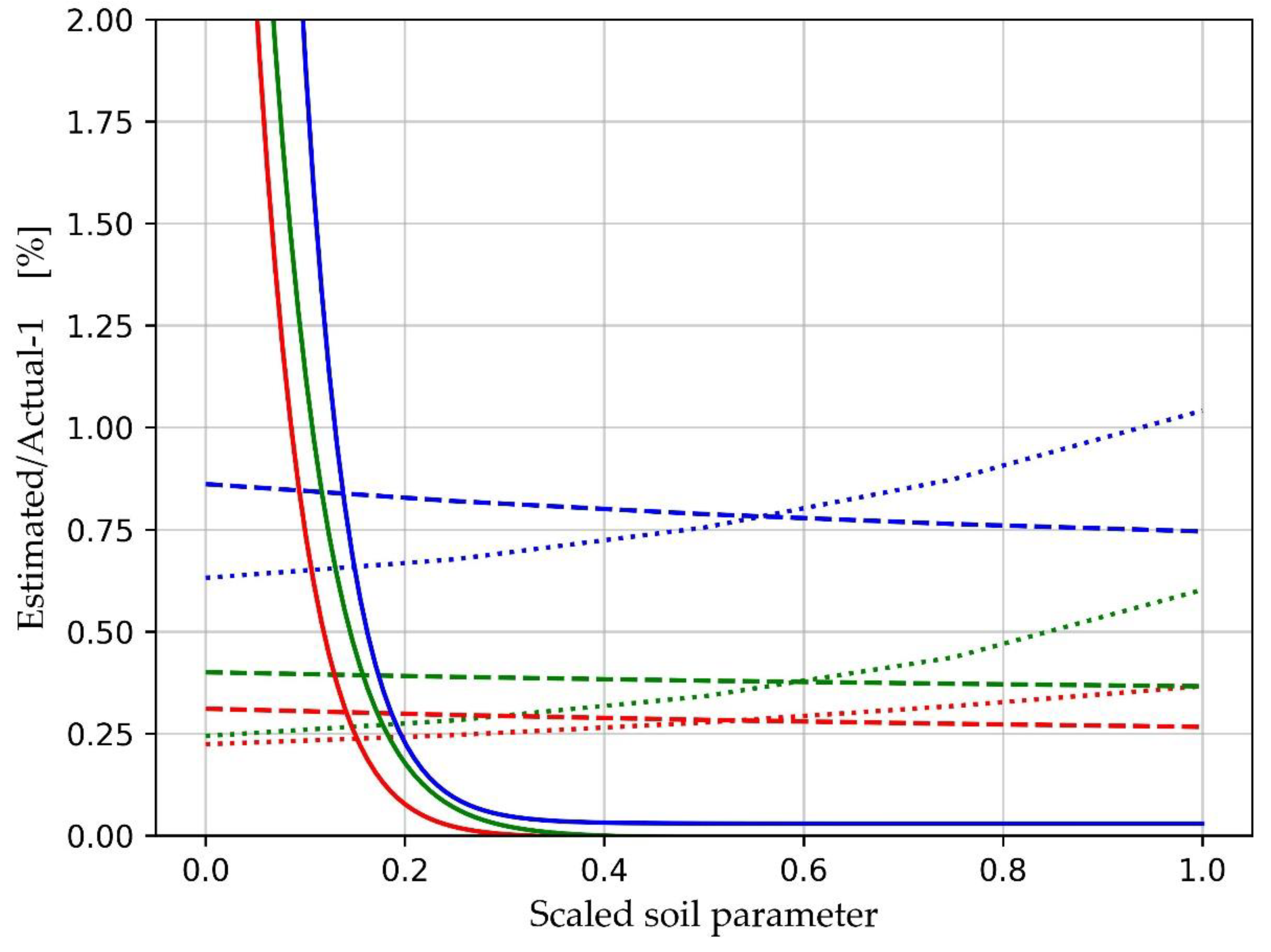

Table 1.
Model parameters.
| Properties of air | Description | Typical value |
| ρ0 | air density | 1.2 kg m-3 |
| η | dynamic viscosity of air | 18.5e-6 Pa s |
| Design parameters | ||
| θ | angle of incidence | 0° - 40° |
| f | acoustic frequency | 1 – 25 kHz |
| Physical properties of soil | ||
| 𝜙 | porosity | 0.6 |
| α∞ | tortuosity | 1.4 |
| rpore | pore radius | 30 – 180 μm |
| Derived quantities | ||
| X | tan2(θ) | 0 – 0.7 |
| fc | critical frequency | 0.5 – 22 kHz |
| Ω (f = 50 Hz) | normalized frequency | 0.002 - 0.1 |
| Ω (f = 25 kHz) | normalized frequency | 1 - 50 |
Table 2.
Measured values of |R|.
| θ | |||||
| 0° | 10° | 20° | 30° | ||
|
f kHz |
4 | 0.437 | 0.433 | 0.419 | 0.393 |
| 5.04 | 0.413 | 0.409 | 0.396 | 0.373 | |
| 6.35 | 0.395 | 0.392 | 0.380 | 0.358 | |
| 8 | 0.382 | 0.379 | 0.368 | 0.349 | |
| 10.08 | 0.373 | 0.370 | 0.361 | 0.342 | |
| 12.70 | 0.367 | 0.365 | 0.355 | 0.338 | |
| 16 | 0.364 | 0.361 | 0.352 | 0.335 | |
Table 3.
Errors in parameter estimation averaged over all soil profiles.
| Physical properties of soil | Biasβ% | Uncertainty s % |
| porosity | 0.29 | 0.45 |
| tortuosity | 0.80 | 0.89 |
| pore radius | 0.38 | 0.38 |
Disclaimer/Publisher’s Note: The statements, opinions and data contained in all publications are solely those of the individual author(s) and contributor(s) and not of MDPI and/or the editor(s). MDPI and/or the editor(s) disclaim responsibility for any injury to people or property resulting from any ideas, methods, instructions or products referred to in the content. |
© 2025 by the authors. Licensee MDPI, Basel, Switzerland. This article is an open access article distributed under the terms and conditions of the Creative Commons Attribution (CC BY) license (http://creativecommons.org/licenses/by/4.0/).
Copyright: This open access article is published under a Creative Commons CC BY 4.0 license, which permit the free download, distribution, and reuse, provided that the author and preprint are cited in any reuse.


