Submitted:
08 August 2025
Posted:
12 August 2025
You are already at the latest version
Abstract
In this paper, we consider thermodynamic single-phase closed systems under isothermal and isobaric conditions. The state of such systems is characterized by parameters such as pressure, composition, etc., which are called degrees of freedom of the system. If the system is in thermodynamic equilibrium, then for these parameters, the value of the Gibbs function, DG, reaches a minimum value equal to the sum of the weighted chemical potentials of the individual components. The presented work shows that in complex chemical systems there may be many sets of chemical potentials giving the same value of DG, i.e., the equilibrium state is degenerate. A relationship between the maximum value of the degree of degeneracy and the composition has been found. From a topological point of view, the state of the system is represented by a planar graph lying on the surface of the topological manifold DG, formed by a path/paths of minimum length connecting all degrees of freedom of the system (vertices of the graph). Individual paths are a concatenation of edges connecting successive pairs of degrees of freedom. The length of the graph edges is equal to the weighted value of the chemical potential of the corresponding component of the system. The number of paths increases rapidly with the increase in the number of components of the system. The number of paths of minimum length depends on the configuration of the degrees of freedom of the system. In the study of model ternary systems with randomly selected 51 configurations of degrees of freedom, it was shown that in such systems only about 75% of configurations have one path of minimum length, while the rest are characterized by the existence of two or more minimum or near-minimum paths. This indicates that among ternary systems there are some in which the equilibrium state is degenerate. According to the topological representation of equilibrium states in complex systems, the degeneration of these states is a consequence of the existence of a large number of paths in such systems.
Keywords:
thermodynamic equilibrium
; Gibbs potential
; chemical graph
; planar graph
; Euler's formula
1. Introduction
Isobaric–isothermal equilibrium (p, T = const) in closed chemical systems with C components (mole fractions of the components: x1, x2…,xC) is described by the Gibbs potential ΔG(p, T, x1, x2, …,xC). The set of values of an n-variable function in topology is called the topological manifold of that function. The function ΔG is a homogeneous function of degree one with respect to the concentrations xi, which allows it to be represented in the form [1]:
where μi is the chemical potential of the i-th component:
ΔG = μ1*x1 + μ2*x2 + μ3*x3 +…+ μC*xC
Until now, thermodynamic studies have tacitly assumed that each equilibrium state, described by the minimum value of ΔG, corresponds to only one set of chemical potentials of individual components: {μι ; i=1,…,C }. This is equivalent to the statement that the degree of degeneracy of each thermodynamic equilibrium state is equal to one, i.e., the state is non-degenerate. When the number of sets of chemical potentials satisfying Eq. (1) for a given value of ΔG is greater than 1, then such a state will be degenerate. Its degree of degeneracy ηΔG is the number of different sets {μι }, corresponding to the same value of ΔG. When looking for arguments in thermodynamics that support degeneration, we compare the total differentials of the function: ΔG(p, T, x1, x2, …,xC) and the same function expressed by equation (1). This comparison convinces us that the sum of weighted changes in chemical potentials is zero, which is known as the Gibbs-Duhem theorem [1]:
(x1*dμ1+x2*dμ2 +x3*dμ3 +..+ xC*dμC) = 0
Consequently, due to the composition, the homogeneity of the Gibbs function combined with the imposition of the Gibbs–Duhem equation (3) onto the ΔG potential enforces C - 1 constraints on the Gibbs function. These constraints are defined by Equation (4):
After taking into account the C-1 relationship between the thermodynamic parameters (see Eq. 4) characterizing equilibrium, we conclude that the topological manifold of the Gibbs function is a simple two-dimensional surface immersed in a C+1 dimensional space.
Specifically, it will be a 2-D piecewise smooth surface. Figure 1 shows an example of topological manifold for binary systems. The smooth fragments of this surface represent the individual phases of the system: (α, β, γ, δ). The lines where these fragments intersect are the lines of interphase equilibrium. The points on the pieces of the manifold are a classical representation of equilibrium states. Here, we can distinguish between: points lying inside a smooth fragment of the manifold, which represent equilibrium in single-phase systems (in Figure 1, this is, for example, the point marked R = (p, T, x1, x2, … , xC) ); points lying on the intersection line of two smooth fragments – representing interphase equilibrium (in Figure 1, this is, for example, the point marked r); and the common point of all smooth fragments of the manifold – which represents the invariant state of the system (in Figure 1, this is the point marked R* = (p*, T*, x*1, x*2, …,x*C) ). At these points of the manifold, in particular at point R, the Gibbs function reaches its minimum value. This means that any change in the component of point R will cause an increase in ΔG. Let us note here that in this work, we will only be interested in equilibria in single-phase systems. At first glance, it is difficult to see in the classical representation of equilibrium, R = (p, T, x1, x2, … , xC), any suggestion of the existence of degeneration of such states. However, it is worth noting that the Gibbs-Duhem theorem states that if the set of chemical potentials {μι ; i=1,…,C} represents an equilibrium state with Gibbs potential ΔG, then another set {μi’ ; i=1,…, C} also represents the same state, provided that: μi’ = μi + δi , and the weighted sum of all δi is equal to zero (see: Eq.3). This leads to the conclusion that at the equilibrium point, the value of ΔG does not change, but the immediate vicinity of this point may change, such that if the potentials μι increase along some axes, they will decrease along other axes, so that the sum of the weighted potentials (i.e., ΔG ) remains unchanged. This can lead to two conclusions:
1) equilibrium states may be degenerate;
2) the topological manifold of the function ΔG is not a static surface, but may undergo synchronized oscillation around the equilibrium point. Synchronization causes the sum of weighted derivatives after the composition xi of the function ΔG to always be the same, although this corresponds to different sets of derivatives ΔG (i.e., μι and μi’).
Let us summarize: the classical representation of equilibrium allows for the existence of degeneration of this state, although it does not specify what the degree of degeneration will depend on or how to calculate it. These issues will be analyzed later in this paper. In order to avoid the accusation that the problem is being examined from only one point of view on equilibrium, we will seek answers to the questions posed above by considering an alternative representation of thermodynamic equilibrium. This will be the topological representation of the equilibrium state. To move to it, let us first denote the geodesic coordinates of smooth 2-D fragments of a topological manifold, representing individual phases of the system, with the symbols X and Y. Naturally, both coordinates are functions of thermodynamic parameters. The important aspect is that the values of these coordinates create a lattice of geodesics on the topological manifold of the Gibbs potential for a given phase of the system. The geodesic lattice R = R(X,Y) can be said to represent the topological manifold of the Gibbs function of a given phase of the analyzed systems. Because the function ΔG is continuous for a given phase, the topological manifold R for a single phase is a continuous and smooth geometric construct (e.g., with no holes or sharp changes in value). On a topological manifold defined in this way, the representation of equilibrium states must satisfy the Gibbs phase rule [1]:
where f – number of degrees of freedom in a thermodynamic system, C – number of independent components; and p – number of phases.
f = C – p +2
In this way, we have approached a topological representation of equilibrium states. This representation arises as a consequence of the similarity of the thermodynamic relation (5) to the well-known Euler equation from topology and graph theory [2]. It describes the relationships between the numbers: of vertices- V, edges- E, faces - F (see Eq. 6):
in planar graphs lying on 2-D surfaces isomorphic to the plane.
F = E – V +2
In equilibrium thermodynamics, the correspondence between thermodynamic relation (5) – concerning real chemical systems – and equation (6) – concerning abstract topological objects – was first noticed about 100 years ago [3, 4]. Since then, it (this correspondence) has been the subject of analysis by various research groups [5,6,7,8,9,10,11,12]. The final result of these analyses is the conclusion that thermodynamic equilibrium in closed systems must be represented by a planar state graph lying on a 2-D surface isomorphic to a plane. It has been established [13] that the parameters characterizing equilibrium are assigned to the parameters of the state graph as follows:
f ↔V, p ↔ F, C ↔ E.
Currently, assigning degrees of freedom, f, to the vertices of the graph, V, and individual phases, p, to the edges of the graph, F, seems natural and uncontroversial. After all, can there be any objection to the claim that the points forming smooth pieces of a topological manifold will represent the faces of the state graph? Or that degrees of freedom, f, are represented by the vertices, V, of this graph? Although here, a layman may have doubts, after all: “every point on a 2-D surface has two degrees of freedom, and each thermodynamic degree is only one.” This doubt will disappear if we take into account the fact that the values of the Gibbs function, G, are always given relative to a certain reference state, G*. From a topological point of view, the only natural reference state for each point on the surface of a topological manifold is the invariant state, R* [13]. Therefore, the coordinates of the equilibrium state, R, should also be given relative to this state. Thus, in the topological representation, the equilibrium coordinate, R, is projected onto the position of the reference state, R*. Let us explain this projection at a basic level: “let the point R = (x, y, z), while the reference point has coordinates R* = (a, b, c). Then the position of point R relative to the reference point is represented by the set R1, R2, R3, where: R1 =(x, b, c), R2 =(a, y, c), R3 =(a, b, z)”. Thus, we obtain the i-th component of the projection of any state, R, onto the reference state by replacing the i-th coordinate in R* with the value of this coordinate in R. In this way, in the topological description, the equilibrium state on the surface of the topological manifold of the Gibbs function:
represented by a set of points: R1, R2, R3, R4, …, Rf , where Ri :
etc., while X and Y are functions describing a smooth 2-D fragment of a topological manifold.
ΔG = R(X, Y)
R1 = (X1, Y1) ; X1 =X(p, T*, x1*, …xC*); Y1 =Y(p, T*, x1*, …xC*)
R2 = (X2, Y2) ; X2 =X(p*, T, x1*, …xC*); Y2 =Y(p*, T, x1*, …xC*)
Figure 2 shows, for example, the location of the vertices of the state graph for phase α of a three-component system. The vertices of the state graph defined in this way will have only one degree of freedom. As noted in the introduction to this work, we are only interested in single-phase systems (p = 1). Therefore, Eqs. 5 and 6 inform us that the state graphs for such systems have only one face (i.e., they lie on it) and the number of edges in them (E) is equal to the number of components of the system (C).
Furthermore, the number of vertices (V) in such state graphs is one greater than the number of edges. It follows from the above that equilibrium in C-component single-phase systems is represented by a (C + 1)-vertex tree lying on a smooth fragment of the topological manifold of the Gibbs function, ΔG. This leads to the conclusion that such a tree is formed by connecting C+1 vertices with a sequence of C edges of minimum length. If the number of vertices/degrees of freedom, V, is greater than 2, then there are V*(V+1)/2 edges connecting individual pairs of vertices. For example, for ternary systems there are 6 such edges (see Figure 3), and for quaternary systems there are as many as 10. According to Eqs. 5 and 6, an edge represents a certain property of the corresponding component of the system. The state of the entire thermodynamic system is represented by sequences C = V-1 of edges connecting successive vertices. As mentioned above, in topology such sequences of edges are called paths of a graph (for ternary systems, see Figure 4). A path that describes the thermodynamic equilibrium corresponding to the value ΔG will obviously have a minimum length. The dependence Eq. (1) unambiguously suggests that the properties assigned to the edges forming the path should be weighted chemical potentials of the components, xk*μk.
This leads to the conclusion that the aforementioned edges will be geodesic lines connecting individual vertices of the graph, Ri, Rj:
because only the sum of the lengths of the geodesic lines can give a graph with the minimum path length representing the state of equilibrium, ΔG:
So we are in the following situation: on a 2-D surface, we have V vertices connected by a path consisting of V-1 edges selected from among V*(V+1)/2 edges. It is obvious that there can be more than one such path. How many of them will have a minimum length or a length close to it? For example, for single-component systems, there is only one such path, and it will simply be the edge e12=(R1-R2) connecting both vertices. This edge has the minimum length, i.e., it will be a geodesic line. In binary systems, there will be three paths running through 3 vertices: e12 – e23 , e21 - e13, e13 – e32. Regardless of which of them will have the minimum length, and how many such paths there will be, they will form, as in unary systems, a linear tree. In this example, the search for minimum paths does not seem too burdensome, because we are only examining 3 paths. Unfortunately, in order to perform such research, it is necessary to know the topological manifold of the Gibbs function (see Eq. 12), which is the only obstacle to performing the research. For more complex systems, there are more obstacles. Take, for example, ternary systems, as shown in Figure 4, where there are 16 paths that can be drawn through 4 vertices. Twelve of them are 4-vertex linear trees (without branches), and four are branched trees [14]. To represent them, let us introduce unindexed edge labels (a, b, ...). So instead of the labels:
the edges will be marked as follows:
e12 , e13 , e14 , e23, e24, e34
a, b, c, d, e, f
Individual 3-edge paths running through 4 vertices will be either linear trees (12 paths)[14]:
or branching trees (four paths):
adf, bde, aef, bfe, ced, cfd, abf, acf, ecf, dac, bae
ade, cef, abc, dba
In [13], single-phase states represented by linear trees are called normal states, while branched trees represent states called exotic states. Thus, in order to determine which graphs describe thermodynamic equilibrium, it is necessary to calculate the path lengths for 16 trees. As a side note, let us note that in three-component systems, we can expect the existence of both types of equilibrium mentioned above. For four-component systems, the number of paths increases to 125. Among these paths, nlt = 60 will form linear trees, nbt1 = 60 will form branched trees of the first type, and nbt2 = 5 will form branched trees of the second type. Thus, in four-component systems, we should observe three types of states in single-phase systems in the ratio: 0.48 : 0.48 : 0.04. This ratio gives the probabilities of occurrence of a given type of state. Figure 5 shows the probabilities of individual types of states (including equilibria) in three- and four-component systems. As can be seen in Figure 5, an increase in the number of components, C, causes an increase in the probability of exotic states and a decrease in the probability of normal states. The figure also shows graphs representing states in the systems discussed. The quantity denoted by the symbol η corresponds to the number of all paths. This number increases monstrously with the increase in the number of vertices, and thus also with the increase in the number of components of the system. J.V. Knop et al. [14] state that its value is equal to: η = (C+1)(C-1). Such a large value of η is the second obstacle (the first being ignorance of topological manifold) to the use of topological representation in the description of equilibria in complex systems.
For the equilibrium state of complex systems, among this huge number of paths, is there only one with a minimum length, or are there more? The answer to this question is equivalent to answering the question: “Does the topological representation of thermodynamic equilibrium allow for the existence of degenerate states?” There is only one answer: yes, the topological representation suggests that degenerate equilibrium states can exist. They can exist because for systems with a large number of components, C, it is unlikely that there is only one path of minimal (or very close to minimal) length connecting C+1 vertices. Later in this paper, we will discuss the justification for the thesis contained in the last sentence. For now, however, we will devote a few words to the relationship between classical and topological representations. One might ask: “Why bother, if it is clear that both representations allow for the degeneration of equilibrium states, albeit in different ways?” The answer is that analyzing this relationship will allow us to formulate both the necessary and sufficient conditions for the degeneration of states more precisely. Note that the classical representation states that two (or more) states characterized by the following sets of chemical potentials: {μι ; i=1,…,C}, {μi’ ; i=1,…, C} will describe the same equilibrium if the weighted sum of xi*μι is equal to the weighted sum of xi*μι‘ (see Eq. 3). However, the topological representation additionally requires that the individual components in both sums represent the lengths of the corresponding edges in the graph of states, i.e., that they satisfy Eq. 11. Therefore, we claim that the classical representation provides only a necessary condition, while the topological representation provides a necessary and sufficient condition for the degeneracy of the equilibrium state. So much for the introduction, now let’s move on to specifics, such as answers to questions: how to calculate the degree of degeneracy of the equilibrium state? What parameters does it depend on? In which systems is the probability of degeneracy higher? , etc.
2. Theory
To answer the questions: whether the state of thermodynamic equilibrium is degenerate and what is its degree of degeneration, we must determine:
-first, how many different sets {μk, k = 1, 2, ..., C} such that substituting the chemical potentials, μk , into Eq.1 gives the same value of ΔG for these sets;
and,
-second, whether the sets of weighted chemical potentials satisfying the previous condition represent the lengths of the individual edges eij(k) of the state graph:
The number of chemical potential sets satisfying only the first condition is the maximum value of the degree of degeneracy of the equilibrium state, . The actual value of this degree, , is obtained by rejecting those sets that are excluded by the second condition. To indicate which sets will be excluded for the system under consideration, we need to know the equation of the topological variety of the Gibbs function ΔG = R(X, Y), because it defines the lengths of the individual edges of the graphs (see Eq. 11). Unfortunately, even for relatively simple systems (binary, ternary), this quantity is unknown. Therefore, using the tool of classical representation of equilibrium states, we will be satisfied with calculating only . Once we have this value, we will see what the “lame” topological representation says about the value of (the epithet ‘lame’ was used by analogy to a “lame duck”). It is “lame” because in this tool we only know the anatomy of individual paths (i.e., we know how individual edges are arranged in trees), but we do not know the form of the topological manifold of the Gibbs function on which these paths lie. Without knowing the form of the surface R(X, Y), does information about how individual paths (trees - potential equilibrium state graphs) lying on it are constructed expand our knowledge about the degrees of degeneration of equilibrium states? Let’s check it out.
2.1. The Maximum Value of the Degree of Degeneration of the State of Thermodynamic Equilibrium
In classical thermodynamics, the quantitative equilibrium in the C-component isobaric-isothermal system is determined by the minimum value of the Gibbs potential measured in relation to a certain reference state, ΔG (see Eq. 1). In the following considerations, we will assume that there are ηΔG of different sets of chemical potentials {μ’i (k), i = 1,2, ..., C; k = 1,2, .., ηΔG} such that for each set μ’i, the weighted sum in Eq. 1 is equal to the Gibbs function. Hence, ηΔG, will be the degree of degeneration of the equilibrium state. How to calculate this parameter? To answer this question, let us note that in our search we should take into account two conditions [15]. First, we are looking for a C-element set of numbers, μ’i, whose weighted sum (Eq. 1) gives the same value as the set, {μi}. Secondly, each product of numbers, xiμ’i should be equal to the distance between the corresponding vertices in the state graph. Since for abstract states of systems we do not know the specific form of the topological manifold, let alone the position of individual vertices in the state graph, we can say that the second condition practically excludes the possibility of calculating ηΔG . However, in order not to be content with this inability, we will continue to try, taking only the first condition into account, to calculate the maximum degree of degeneration .
Of course, a parameter defined in this way may drastically overestimate the real degree of degeneracy, because its calculations also take into account such edges in the state graph that do not connect the real vertices-degrees of freedom of the system. In the presented calculations, the properties of the Heaviside function, h(x), and the Dirac delta δ(x) will be used. Specifically, we will use the following properties of these functions [30]:
The integral of the second of these functions will be different from zero only if the region of integration contains 0. If we integrate a Dirac delta function whose argument depends on many variables then the value of the integral will be equal to the number of zeros of the argument.
Let us assume that the set of chemical potentials corresponds to me, according to Eq. 1, the values of ΔG. Let us denote by the symbol Mi the quotient:
It is easy to verify that the values of this parameter meet the following condition:
We will now write the dependence Eq.1 as:
1 = Μ1*x1 + Μ2*x2 + Μ3*x3 +…+ ΜC*xC
The maximum value of the degree of degeneracy, of the classical state of equilibrium, will be equal to the number of sets Mi satisfying the equality:
[1 − (Μ1*x1 + Μ2*x2 + Μ3*x3 +…+ ΜC*xC)]=0
This number will be equal to the integral of the Dirac delta function:
where: mi = xi*Mi .With the above integration limits after m1, the argument x of the delta Dirac function δ(x), satisfies the condition:
So the integral over m1 is going to be equal to .
Thus, the equation 26 as a result of integration after m1 takes the form:
The integral over the variable m2 gives:
The integral over the variable m3 gives:
Successive integrations finally lead to the following result:
Equation (29) shows that the maximum value of the degree of degeneration of the thermodynamic equilibrium state depends only on the phase composition, and is greater the more components in this phase are present at low concentrations. This parameter reaches the minimum value at equal concentrations of the system components. Unfortunately, the value of this parameter is not equal to 1, which would indicate no degeneration. Due to the above-mentioned shortcomings of this coefficient, its calculated value also does not prove the existence of degeneration, but only suggests its presence in some equilibrium states. The question is: How much does the calculated parameter differ from the actual degree of degeneration? The writer of these words does not know the answer to this question, but he thinks that he knows what path to look for (this answer). Now let us note that the path set is composed of two subsets. One is a subset of minimum length paths through all the vertices of the graph; the second are paths of a different length (greater than the minimum) also passing through all the vertices. On the other hand, the set is also composed of two subsets. In both subsets the lengths of the paths are the same, but in one subset the paths run through all the vertices (degrees of freedom) of the graph, and in the other the paths omit at least one vertex in the state graph. Thus, the actual degree of degeneration of the thermodynamic equilibrium state, , will be the number of elements in the intersection of the two sets mentioned above. The question is how to find the common part of these sets?
We will not find the answer to this question as long as we only have a flawed topological representation. The situation seems to be at a stalemate, because ignorance of topological manifold (and thus also the lack of a reference state) entails not only uncertainty about the position of individual degrees of freedom of the system, but also a lack of clarity about the configuration of vertices (i.e., degrees of freedom). The consequence of this situation is the inability to determine the position and length of the edges that make up the paths. Let us assume for a moment that we know the lengths of all the edges, eij, that make up the individual paths. Does this solve the problem in any way? For example, will knowing the lengths of all the edges allow us to determine the configuration of the vertices? The answer is “yes, but it will not necessarily be a configuration corresponding to the equilibrium state.” Since one vertex configuration, Nconfig = 1, corresponds to one set of individual edges, we should consider not one, but a large number of edge sets, Nconfig →∞. Then, among the configurations obtained, some will correspond to equilibrium states. Which ones? At present, the author does not know of a criterion that would allow us to isolate from the obtained vertex configurations those that represent equilibrium states.
With this assumption, the further procedure will be as follows:
1. We assume that for the considered vertex configurations, Nconfig = 1, 2, 3,.., the lengths of randomly selected edges do not exceed a certain maximum value: eij < emax, i.e. eij =random(emax), where random() is a pseudorandom number from the interval (0, emax).
2. Using pseudorandom number generators, we determine the lengths of individual edges (see, e.g., Eq. 14).
3. The edge lengths are used to calculate the sets of path lengths for a given vertex configuration (see Eqs. 15, 16).
4. For each configuration, we find the path with the minimum length and lengths that differ negligibly from it.
5. We will consider that the minimum and almost minimum paths represent a single state of thermodynamic equilibrium.
Now, let’s look at a specific example of a three-component system.
2.2. The Number of Minimum Paths Connecting Degrees of Freedom of a Ternary System on a 2-D Surface.
Each path is a concatenation of edges connecting individual pairs of points, i.e., the vertices of the graph. The length of each edge is determined by the coordinates of the vertices connected by that edge (Eq. 11). In the model calculations presented here, the coordinates will be selected randomly. This means that the lengths of the edges will also be random. Therefore, it seems reasonable to skip the step of selecting the positions of the vertices, as described earlier, and proceed directly to the random selection of the lengths of the edges in the paths connecting the V vertices under investigation. Let me just remind you that the vertices are the degrees of freedom of the system. Thus, for single-phase systems, V = 2; for binary systems, V = 3; for ternary systems, V = 4; for four-component systems, V = 5; etc. As follows from [14], V vertices on the surface of a 2-sphere can connect (V)V-2 non-isomorphic paths. So, for the systems mentioned above, this will be, respectively: 1; 3; 16; 125; etc. paths. To examine the ordering of path lengths in individual systems, we will discard unary and binary systems (too few paths) and, first, focus on ternary systems. In these systems, the concatenation of three (out of 6 possible) edges of randomly selected lengths creates 16 different paths [14] (see Eqs. 15, 16). The concatenations with the shortest length therefore represent the state of thermodynamic equilibrium in our ternary systems. Thus, according to the notation in Figure 3, individual concatenations will be denoted by the appropriate sequence of letter symbols: (abc..), where a, b, c,…, are edges connecting points on a 2-D surface. Let |(abc…)| denote the length of the path formed by a given sequence of edges. Obviously, this length will be equal to the sum of the lengths of the individual edges. So we are looking for all those concatenations (a’b’c’..) whose length is minimal or negligibly different from the minimum (abc...)min
(|(a’b’c’..)| - |(abc...)min|) =δ →0
The term “negligibly small” should not raise any objections, considering that the state of equilibrium of the system under consideration consists of sets of microstates that differ slightly in their thermodynamic parameters. It seems that the issue that may raise doubts is the choice of a specific value for this “negligibly small difference δ.” In the rest of this paper, we will assume that this will be the case when δ < 5% of the length of the shortest path. Optimistically, we will argue that the path of minimum length, together with those that differ negligibly little from the minimum, will represent the same state of thermodynamic equilibrium. Thus, if concatenations of edges with the aforementioned properties exist, then the topological representation will indicate that the thermodynamic equilibrium state of the system is degenerate.
For the initial test, 51 configurations (Nconfig = 51) of four points (graph vertices) lying on a smooth two-dimensional surface were selected, which are connected by three of the six edges (a, b, c, ...) of randomly selected lengths. The question may arise: “Why were 51 configurations chosen?” The answer is so trivial that it is almost ridiculous: “Because the results of the calculations for so many configurations still fit on an A4 page and can be taken in at a glance.” In each set of the aforementioned 51 configurations, the randomly selected edge lengths |eij| were as follows: in the first set, they were no greater than 30; in the second set, no greater than 10; in the third set, no greater than 5; in the fourth set, no greater than 3; and in the fifth set, no greater than 1. The random lengths of individual edges were determined using pseudo-random number generators from MS Excel (2007) or a spreadsheet from Libre Office Calc (ver. 25.2). The results obtained for the last three sets are given in the Appendix to this paper. However, Table 1 and Table 2 present the results for vertex configurations that allow for the existence of edges with a maximum length of 30 and 10, respectively. Table 3 and Table 4 contain the lengths of all 16 paths calculated for both sets. These lengths are normalized to the length of the minimum path. Thus, trees corresponding to paths of length 1,000 represent a state of thermodynamic equilibrium. Such trees will be equilibrium graphs. Paths much longer than 1 correspond to states far from equilibrium. There are always 51 graphs in both sets of state graphs, i.e., as many as there are vertex configurations/degrees of freedom in the set. However, this does not necessarily mean that the topological representation of equilibrium states indicates the absence of degeneration, as among all paths in both sets there are also those whose lengths differ negligibly from 1,000. The lengths of such paths in Table 3 and Table 4 are shaded in gray.
From these tables, we can see that in most cases, the length of the shaded paths differs from 1.000 much less than the limit value of δ =0,05 adopted here. There are 25 such paths in Table 3 and 15 in Table 4. It is easy to see that shaded paths usually appear in configurations where at least one edge is significantly shorter than the other edges. Incidentally, this explains why the classical representation of equilibrium maintains that in chemical systems with a very low content of one or more components, the degree of degeneration of the equilibrium state will be higher than in systems with other compositions. All the most important properties of the paths for the 5 sets of configurations discussed (two from Table 3 and Table 4 and three from the tables in the Appendix) are given in Table 5. This table shows that in the systems under consideration, the state of thermodynamic equilibrium is represented by a linear tree more often than by a branched tree. However, as we can see in Table 5, the ratio of the number of linear trees of minimum length to the number of all minimal trees is close to 0.75, i.e., the fraction of linear paths in the total number of paths: nlt / (nlt+ nbt). Is there a reason that determines the proportions of individual types of single-phase equilibria in complex systems? Analysis of 3- and 4-component systems indicates that this reason may be the fact that the total anatomy of individual path types is independent of the path type. This means that for a given configuration of vertices, the shares of individual edges in all paths of a given type are independent of the type of paths (i.e., in all linear paths, the proportion of the number of individual edges is identical to that in individual types of branched paths). We will further assume that the relationship between the proportions of individual types of single-phase equilibria discussed above is valid for more complex thermodynamic systems. In single-phase C-component systems, characterized by V = C +1 degrees of freedom, the number of paths forming a linear tree is equal to half the number of V-element permutations (because the permutations [beginning, ……, end] and [end, ….., beginning] form isomorphic paths = indistinguishable). Therefore, in systems composed of a large number of components, the fraction of equilibria represented by linear trees, ρlt will be equal to:
i.e., negligibly small.
This relationship shows that in the systems discussed, fewer and fewer equilibrium states are represented by linear trees, and more and more by branched trees, so these equilibria will most often be exotic equilibria, not found in unary and binary systems. I believe this is an interesting conclusion for chemists, but let us return to the main focus of this work, i.e., the question of whether thermodynamic equilibrium states can be degenerate.
The data in Table 5 show that only one minimum path, N1, characterizes approximately 40 of the 51 analyzed configurations of degrees of freedom in individual data sets. The remaining configurations have at least two such paths. The numbers in this table also show that the fraction of the number of configurations with two or more paths to the total number of configurations (i.e., 51) is approximately equal to the fraction nbt /(nlt+ nbt), which characterizes the proportion of branched paths in their total number. To explain this somewhat strange relationship, note that two or more minimal paths N = (N2 +N3 +…) can only appear in certain configurations of degrees of freedom. These configurations generally allow for the existence of different families/types of paths (linear, branched1, branched2, …, etc.). The size of the family, i.e., the number of paths in this family, is denoted by: nlt, nbt1, nbt2,… . I think it will be obvious to state that the number of minimum paths in a given family, N, should increase with the size of the family. For 3-component systems, this statement is confirmed by the results presented in Table 5. In my opinion, this is a fairly strong argument provided by topology in favor of the existence of degeneracy of equilibrium states in complex thermodynamic systems. This strong argument would be clear evidence of the existence of degeneracy if we were certain that all the vertex configurations obtained by the method described above correspond to equilibrium states. As mentioned earlier, when the set of configurations under study is sufficiently large, Nconfig →∞, then this set (let us call it a mixed set) will contain both configurations representing equilibrium and those not representing such a state. Since there is no known criterion that would allow us to extract equilibrium configurations from such a set, we must be content with the assumption that the properties of minimal paths established above for the mixed set are also true for the set of equilibrium configurations. This means that, for example, we reject the assumption that among the configurations under consideration, only those that have a single minimal path are equilibrium configurations.
3. Summary
In this work, using classical and topological representations of thermodynamic equilibrium, it was shown that in complex systems such a state can be degenerate, i.e. several sets of chemical potentials can be assigned to one minimum value of the Gibbs function. The maximum number of such sets, i.e. the maximum value of the degree of degeneration, was calculated (see equation 29). It is shown that some configurations of degrees of freedom of three-component systems allow for the existence of degeneracy of 2 and higher orders of equilibrium states. The configurations of degrees of freedom allow for the existence of many families of paths connecting individual degrees. Those families that contain more paths will prefer degenerate states. Another conclusion from the analysis of the results presented in the paper is that as the number of components in single-phase systems increases, so does the number of exotic equilibrium states that differ in their topological description (state graph = branched tree) from normal states (state graph = linear tree) occurring in single- and two-component systems. Finally, I would like to propose a name for degenerate equilibrium states; it seems that “chemical chimeras” would be an appropriate name.
Appendix
This part of the work contains 6 tables with the results of path length calculations for 51 configurations in which emax is equal to 1, 3, 5, respectively.

Table A6.
The length of individual edges, eij , of trees lying on a surface isomorphic to a 2-D plane. The edges connect 2 of the 4 points in Nconfig = 51 randomly determined configurations consisting of four points. The maximum length of any edge, eij , does not exceed 1. The lengths eij , are given to 3 decimal places.
| e12 | e13 | e14 | e23 | e24 | e34 | |
| Nconfig | a | b | c | d | e | f |
| 1 | 0,789 | 0,785 | 0,712 | 0,395 | 0,283 | 0,639 |
| 2 | 0,322 | 0,318 | 0,607 | 0,872 | 0,005 | 0,290 |
| 3 | 0,301 | 0,400 | 0,812 | 0,785 | 0,315 | 0,060 |
| 4 | 0,866 | 0,681 | 0,017 | 0,487 | 0,994 | 0,430 |
| 5 | 0,901 | 0,264 | 0,403 | 0,438 | 0,905 | 0,247 |
| 6 | 0,243 | 0,238 | 0,146 | 0,559 | 0,195 | 0,577 |
| 7 | 0,515 | 0,005 | 0,931 | 0,472 | 0,572 | 0,576 |
| 8 | 0,467 | 0,777 | 0,873 | 0,806 | 0,329 | 0,937 |
| 9 | 0,885 | 0,046 | 0,030 | 0,917 | 0,596 | 0,500 |
| 10 | 0,055 | 0,600 | 0,253 | 0,896 | 0,853 | 0,926 |
| 11 | 0,651 | 0,229 | 0,613 | 0,958 | 0,959 | 0,716 |
| 12 | 0,508 | 0,624 | 0,620 | 0,602 | 0,818 | 0,565 |
| 13 | 0,441 | 0,840 | 0,042 | 0,961 | 0,695 | 0,610 |
| 14 | 0,882 | 0,917 | 0,343 | 0,098 | 0,080 | 0,354 |
| 15 | 0,478 | 0,597 | 0,647 | 0,522 | 0,886 | 0,074 |
| 16 | 0,232 | 0,008 | 0,975 | 0,805 | 0,848 | 0,411 |
| 17 | 0,945 | 0,733 | 0,576 | 0,401 | 0,322 | 0,651 |
| 18 | 0,031 | 0,109 | 0,567 | 0,822 | 0,019 | 0,523 |
| 19 | 0,686 | 0,079 | 0,551 | 0,132 | 0,967 | 0,247 |
| 20 | 0,050 | 0,501 | 0,545 | 0,240 | 0,465 | 0,116 |
| 21 | 0,994 | 0,753 | 0,262 | 0,952 | 0,987 | 0,797 |
| 22 | 0,472 | 0,278 | 0,507 | 0,631 | 0,635 | 0,514 |
| 23 | 0,908 | 0,178 | 0,758 | 0,081 | 0,181 | 0,130 |
| 24 | 0,362 | 0,409 | 0,408 | 0,499 | 0,074 | 0,150 |
| 25 | 0,282 | 0,970 | 0,607 | 0,144 | 0,961 | 0,342 |
| 26 | 0,934 | 0,491 | 0,650 | 0,360 | 0,690 | 0,233 |
| 27 | 0,871 | 0,870 | 0,403 | 0,293 | 0,965 | 0,900 |
| 28 | 0,269 | 0,225 | 0,398 | 0,966 | 0,631 | 0,122 |
| 29 | 0,702 | 0,846 | 0,080 | 0,157 | 0,968 | 0,096 |
| 30 | 0,390 | 0,465 | 0,149 | 0,250 | 0,791 | 0,249 |
| 31 | 0,246 | 0,007 | 0,555 | 0,024 | 0,854 | 0,284 |
| 32 | 0,553 | 0,506 | 0,612 | 0,269 | 0,061 | 0,309 |
| 33 | 0,244 | 0,189 | 0,782 | 0,934 | 0,128 | 0,952 |
| 34 | 0,474 | 0,093 | 0,604 | 0,154 | 0,231 | 0,459 |
| 35 | 0,115 | 0,074 | 0,918 | 0,632 | 0,449 | 0,336 |
| 36 | 0,534 | 0,223 | 0,552 | 0,929 | 0,671 | 0,602 |
| 37 | 0,866 | 0,676 | 0,049 | 0,449 | 0,025 | 0,107 |
| 38 | 0,188 | 0,946 | 0,834 | 0,518 | 0,610 | 0,381 |
| 39 | 0,050 | 0,555 | 0,591 | 0,160 | 0,034 | 0,475 |
| 40 | 0,351 | 0,169 | 0,047 | 0,952 | 0,047 | 0,814 |
| 41 | 0,420 | 0,017 | 0,118 | 0,843 | 0,313 | 0,949 |
| 42 | 0,765 | 0,313 | 0,033 | 0,165 | 0,893 | 0,465 |
| 43 | 0,428 | 0,836 | 0,030 | 0,157 | 0,905 | 0,334 |
| 44 | 0,134 | 0,244 | 0,787 | 0,499 | 0,382 | 0,223 |
| 45 | 0,136 | 0,619 | 0,439 | 0,050 | 0,078 | 0,643 |
| 46 | 0,612 | 0,933 | 0,723 | 0,076 | 0,759 | 0,764 |
| 47 | 0,865 | 0,378 | 0,251 | 0,626 | 0,093 | 0,994 |
| 48 | 0,642 | 0,437 | 0,223 | 0,241 | 0,838 | 0,838 |
| 49 | 0,237 | 0,947 | 0,469 | 0,093 | 0,172 | 0,293 |
| 50 | 0,267 | 0,123 | 0,742 | 0,277 | 0,847 | 0,198 |
| 51 | 0,788 | 0,594 | 0,423 | 0,516 | 0,216 | 0,546 |
Table A7.
The length of individual edges, eij , of trees lying on a surface isomorphic to a 2-D plane. The edges connect 2 of the 4 points in Nconfig = 51 randomly determined configurations consisting of four points. The maximum length of any edge, eij , does not exceed 3. The lengths eij , are given to 3 decimal places.
| e12 | e13 | e14 | e23 | e24 | e34 | |
| Nconfig | a | b | c | d | e | f |
| 1 | 0,402 | 2,162 | 1,470 | 1,430 | 0,718 | 0,810 |
| 2 | 1,131 | 1,122 | 0,243 | 2,580 | 0,355 | 1,666 |
| 3 | 0,094 | 2,591 | 1,767 | 2,676 | 0,660 | 0,256 |
| 4 | 2,854 | 0,998 | 0,693 | 1,786 | 0,304 | 0,372 |
| 5 | 0,906 | 1,595 | 2,660 | 2,801 | 0,610 | 0,384 |
| 6 | 0,722 | 2,419 | 2,817 | 2,258 | 2,514 | 0,081 |
| 7 | 0,842 | 0,076 | 0,850 | 1,777 | 2,511 | 0,601 |
| 8 | 2,755 | 0,812 | 2,442 | 0,694 | 1,624 | 0,341 |
| 9 | 0,243 | 2,381 | 1,944 | 2,600 | 1,849 | 1,315 |
| 10 | 2,135 | 2,454 | 0,834 | 0,934 | 2,919 | 0,349 |
| 11 | 0,386 | 0,987 | 2,519 | 2,342 | 0,536 | 0,107 |
| 12 | 2,254 | 2,350 | 2,859 | 1,932 | 0,225 | 1,530 |
| 13 | 2,139 | 2,621 | 0,439 | 1,388 | 2,832 | 0,729 |
| 14 | 1,404 | 0,497 | 1,580 | 2,799 | 0,907 | 0,972 |
| 15 | 1,815 | 0,258 | 2,844 | 0,417 | 1,818 | 2,050 |
| 16 | 1,353 | 2,450 | 1,833 | 2,996 | 1,548 | 1,941 |
| 17 | 2,267 | 0,304 | 2,844 | 0,078 | 2,768 | 2,295 |
| 18 | 2,186 | 2,583 | 1,952 | 0,196 | 0,059 | 2,038 |
| 19 | 1,330 | 2,609 | 1,365 | 0,331 | 1,647 | 1,013 |
| 20 | 0,228 | 2,888 | 1,852 | 1,693 | 2,563 | 2,839 |
| 21 | 0,447 | 2,374 | 2,735 | 1,884 | 2,670 | 2,466 |
| 22 | 0,038 | 2,212 | 1,015 | 0,598 | 2,494 | 2,133 |
| 23 | 0,916 | 0,514 | 0,178 | 1,906 | 0,019 | 1,183 |
| 24 | 1,950 | 0,870 | 2,209 | 0,251 | 2,603 | 2,533 |
| 25 | 2,170 | 2,747 | 0,867 | 2,531 | 2,974 | 1,382 |
| 26 | 2,483 | 1,395 | 1,632 | 1,569 | 1,142 | 1,397 |
| 27 | 2,378 | 1,080 | 1,334 | 2,696 | 2,467 | 1,474 |
| 28 | 1,195 | 0,822 | 0,135 | 1,986 | 0,801 | 2,061 |
| 29 | 0,322 | 0,292 | 0,209 | 0,121 | 1,986 | 2,810 |
| 30 | 1,341 | 2,361 | 0,481 | 2,736 | 2,832 | 2,811 |
| 31 | 0,925 | 1,964 | 0,221 | 1,947 | 2,735 | 1,122 |
| 32 | 2,405 | 1,501 | 1,280 | 2,574 | 1,223 | 0,165 |
| 33 | 0,098 | 1,960 | 2,567 | 1,700 | 1,815 | 0,468 |
| 34 | 1,730 | 1,759 | 0,269 | 1,740 | 2,796 | 0,584 |
| 35 | 1,500 | 0,899 | 1,986 | 0,095 | 2,970 | 1,868 |
| 36 | 0,786 | 2,819 | 1,308 | 0,916 | 2,793 | 0,442 |
| 37 | 1,736 | 1,176 | 2,058 | 0,887 | 0,509 | 2,951 |
| 38 | 1,842 | 2,102 | 1,245 | 1,716 | 0,237 | 1,220 |
| 39 | 0,618 | 2,428 | 2,586 | 2,175 | 0,624 | 0,630 |
| 40 | 0,929 | 0,332 | 1,531 | 2,859 | 2,127 | 2,003 |
| 41 | 1,650 | 2,348 | 1,709 | 2,707 | 1,437 | 2,137 |
| 42 | 1,325 | 1,407 | 0,813 | 2,354 | 0,522 | 1,973 |
| 43 | 2,792 | 2,575 | 2,002 | 1,112 | 1,134 | 0,763 |
| 44 | 2,847 | 0,571 | 2,840 | 0,511 | 1,258 | 1,733 |
| 45 | 2,191 | 0,886 | 2,540 | 0,769 | 2,226 | 2,378 |
| 46 | 0,348 | 1,296 | 2,177 | 2,904 | 1,620 | 2,161 |
| 47 | 2,802 | 2,839 | 1,477 | 2,059 | 0,384 | 1,396 |
| 48 | 2,791 | 2,145 | 1,762 | 1,246 | 2,621 | 0,503 |
| 49 | 2,831 | 2,612 | 0,005 | 0,359 | 1,539 | 2,750 |
| 50 | 1,752 | 1,554 | 0,916 | 1,840 | 2,980 | 1,847 |
| 51 | 0,846 | 1,308 | 2,962 | 2,340 | 1,155 | 1,600 |
Table A8.
The length of individual edges, eij , of trees lying on a surface isomorphic to a 2-D plane. The edges connect 2 of the 4 points in Nconfig = 51 randomly determined configurations consisting of four points. The maximum length of any edge, eij , does not exceed 5. The lengths eij , are given to 3 decimal places.
| e12 | e13 | e14 | e23 | e24 | e34 | |
| Nconfig | a | b | c | d | e | f |
| 1 | 4,495 | 0,205 | 3,163 | 1,271 | 4,182 | 4,383 |
| 2 | 0,975 | 3,643 | 1,002 | 0,299 | 3,382 | 1,815 |
| 3 | 4,633 | 4,461 | 4,873 | 4,557 | 1,247 | 4,075 |
| 4 | 3,874 | 3,095 | 1,804 | 3,480 | 0,229 | 3,576 |
| 5 | 4,908 | 2,251 | 0,998 | 3,974 | 2,028 | 1,016 |
| 6 | 3,818 | 1,419 | 0,624 | 4,935 | 4,606 | 1,472 |
| 7 | 0,746 | 3,550 | 3,343 | 1,744 | 0,611 | 4,096 |
| 8 | 1,408 | 3,505 | 0,672 | 3,719 | 3,936 | 2,385 |
| 9 | 2,611 | 1,472 | 3,808 | 3,223 | 1,663 | 0,245 |
| 10 | 2,617 | 1,062 | 3,772 | 4,067 | 3,609 | 0,990 |
| 11 | 2,495 | 3,719 | 2,631 | 2,534 | 4,407 | 1,990 |
| 12 | 3,491 | 1,132 | 1,123 | 0,896 | 1,461 | 4,561 |
| 13 | 1,060 | 3,697 | 0,049 | 3,126 | 0,880 | 0,302 |
| 14 | 0,875 | 1,883 | 4,364 | 4,387 | 3,248 | 2,974 |
| 15 | 0,863 | 1,573 | 0,622 | 4,139 | 2,299 | 3,573 |
| 16 | 3,108 | 0,465 | 2,136 | 4,999 | 0,271 | 0,225 |
| 17 | 1,929 | 0,939 | 2,074 | 0,793 | 2,809 | 2,495 |
| 18 | 3,351 | 2,446 | 3,283 | 1,834 | 3,861 | 0,630 |
| 19 | 3,898 | 2,639 | 2,750 | 2,505 | 3,252 | 0,532 |
| 20 | 3,276 | 0,973 | 2,150 | 0,704 | 3,791 | 0,239 |
| 21 | 2,145 | 3,706 | 3,376 | 4,005 | 1,385 | 2,125 |
| 22 | 0,408 | 1,761 | 1,235 | 2,988 | 4,419 | 1,271 |
| 23 | 2,297 | 3,883 | 2,198 | 0,517 | 3,355 | 4,692 |
| 24 | 1,729 | 4,024 | 3,469 | 2,421 | 2,883 | 4,461 |
| 25 | 0,346 | 0,647 | 1,681 | 2,153 | 2,648 | 4,756 |
| 26 | 3,832 | 4,396 | 4,748 | 2,398 | 1,350 | 4,011 |
| 27 | 2,186 | 4,887 | 2,975 | 2,326 | 2,555 | 4,313 |
| 28 | 4,576 | 1,846 | 3,675 | 4,721 | 3,669 | 0,976 |
| 29 | 1,753 | 0,397 | 1,072 | 0,975 | 4,870 | 2,606 |
| 30 | 2,840 | 1,984 | 4,851 | 2,434 | 1,924 | 0,204 |
| 31 | 3,874 | 3,675 | 0,283 | 1,530 | 1,237 | 2,487 |
| 32 | 1,456 | 3,157 | 4,527 | 1,117 | 4,147 | 1,524 |
| 33 | 4,536 | 2,664 | 1,978 | 4,791 | 4,112 | 0,242 |
| 34 | 3,807 | 3,548 | 4,009 | 0,097 | 3,742 | 1,740 |
| 35 | 2,057 | 3,398 | 4,809 | 3,581 | 3,356 | 0,968 |
| 36 | 1,331 | 3,795 | 0,238 | 2,085 | 0,747 | 3,752 |
| 37 | 4,898 | 1,633 | 3,297 | 0,432 | 0,935 | 1,058 |
| 38 | 3,788 | 1,906 | 4,377 | 3,861 | 0,748 | 4,144 |
| 39 | 2,580 | 4,354 | 0,475 | 0,214 | 2,081 | 1,020 |
| 40 | 2,520 | 2,408 | 2,863 | 4,386 | 0,798 | 3,377 |
| 41 | 2,609 | 0,611 | 3,156 | 2,948 | 1,117 | 3,435 |
| 42 | 1,328 | 3,299 | 0,523 | 3,843 | 2,924 | 1,876 |
| 43 | 3,973 | 4,588 | 4,965 | 2,053 | 3,323 | 3,662 |
| 44 | 1,444 | 0,708 | 3,116 | 0,308 | 1,349 | 4,554 |
| 45 | 1,249 | 1,975 | 0,832 | 0,510 | 4,796 | 3,520 |
| 46 | 3,027 | 0,937 | 4,951 | 0,126 | 0,616 | 4,910 |
| 47 | 0,908 | 0,144 | 0,597 | 2,330 | 1,136 | 0,357 |
| 48 | 1,499 | 2,295 | 2,221 | 2,925 | 1,158 | 4,060 |
| 49 | 1,025 | 2,866 | 4,590 | 4,079 | 1,391 | 1,145 |
| 50 | 2,875 | 4,540 | 3,760 | 0,430 | 3,716 | 4,528 |
| 51 | 4,001 | 0,345 | 4,228 | 3,290 | 2,867 | 3,273 |
Table A9.
The lengths of paths connecting 4 randomly selected points lying on a 2-D plane. The lengths are normalized to the length of the minimum path. The paths are concatenations of selected 3 edges (a, b, c, ...) from Table App6. Individual edges connect 2 of the 4 points. Paths of minimum length are marked in red. Paths whose length differs negligibly (see equation 30) from the minimum length are shaded in gray. The lengths of the paths are given to 3 decimal places. 0 < eij < random(1)
| Nconfig | adf | bde | aef | bfe | ced | cfd | abf | acf | ecb | dbc | dac | bae | ade | cef | abc | dbf |
| 1 | 1,312 | 1,052 | 1,231 | 1,228 | 1,000 | 1,257 | 1,593 | 1,540 | 1,281 | 1,361 | 1,364 | 1,336 | 1,055 | 1,176 | 1,645 | 1,309 |
| 2 | 2,421 | 1,949 | 1,007 | 1,000 | 2,420 | 2,886 | 1,518 | 1,989 | 1,517 | 2,932 | 2,938 | 1,053 | 1,956 | 1,471 | 2,035 | 2,415 |
| 3 | 1,694 | 2,216 | 1,000 | 1,145 | 2,825 | 2,449 | 1,125 | 1,735 | 2,257 | 2,951 | 2,806 | 1,502 | 2,070 | 1,755 | 2,237 | 1,840 |
| 4 | 1,910 | 2,315 | 2,453 | 2,254 | 1,604 | 1,000 | 2,118 | 1,407 | 1,812 | 1,268 | 1,467 | 2,721 | 2,513 | 1,544 | 1,675 | 1,711 |
| 5 | 1,672 | 1,694 | 2,165 | 1,493 | 1,841 | 1,147 | 1,488 | 1,635 | 1,657 | 1,164 | 1,836 | 2,182 | 2,366 | 1,639 | 1,653 | 1,000 |
| 6 | 2,381 | 1,714 | 1,752 | 1,744 | 1,554 | 2,214 | 1,827 | 1,668 | 1,000 | 1,629 | 1,637 | 1,167 | 1,722 | 1,584 | 1,083 | 2,373 |
| 7 | 1,491 | 1,000 | 1,586 | 1,099 | 1,883 | 1,887 | 1,045 | 1,928 | 1,437 | 1,342 | 1,829 | 1,041 | 1,487 | 1,983 | 1,383 | 1,004 |
| 8 | 1,405 | 1,216 | 1,102 | 1,299 | 1,277 | 1,664 | 1,387 | 1,448 | 1,259 | 1,562 | 1,365 | 1,000 | 1,019 | 1,360 | 1,346 | 1,602 |
| 9 | 3,424 | 2,319 | 2,947 | 1,699 | 2,295 | 2,152 | 2,129 | 2,105 | 1,000 | 1,477 | 2,725 | 2,272 | 3,567 | 1,676 | 1,429 | 2,176 |
| 10 | 2,068 | 2,589 | 2,020 | 2,622 | 2,206 | 2,287 | 1,742 | 1,359 | 1,879 | 1,928 | 1,326 | 1,661 | 1,987 | 2,239 | 1,000 | 2,670 |
| 11 | 1,556 | 1,436 | 1,557 | 1,275 | 1,693 | 1,531 | 1,069 | 1,326 | 1,206 | 1,205 | 1,488 | 1,231 | 1,719 | 1,532 | 1,000 | 1,274 |
| 12 | 1,000 | 1,221 | 1,129 | 1,198 | 1,219 | 1,067 | 1,013 | 1,011 | 1,232 | 1,103 | 1,033 | 1,165 | 1,151 | 1,196 | 1,046 | 1,069 |
| 13 | 1,841 | 2,284 | 1,598 | 1,963 | 1,554 | 1,476 | 1,730 | 1,000 | 1,443 | 1,686 | 1,321 | 1,808 | 1,919 | 1,233 | 1,210 | 2,206 |
| 14 | 2,561 | 2,102 | 2,527 | 2,593 | 1,000 | 1,525 | 4,133 | 3,031 | 2,572 | 2,606 | 2,540 | 3,608 | 2,036 | 1,491 | 4,112 | 2,627 |
| 15 | 1,000 | 1,866 | 1,339 | 1,449 | 1,914 | 1,158 | 1,069 | 1,117 | 1,983 | 1,644 | 1,534 | 1,825 | 1,756 | 1,496 | 1,603 | 1,110 |
| 16 | 2,224 | 2,552 | 2,291 | 1,947 | 4,037 | 3,366 | 1,000 | 2,486 | 2,813 | 2,746 | 3,090 | 1,671 | 2,896 | 3,432 | 1,866 | 1,880 |
| 17 | 1,537 | 1,120 | 1,476 | 1,312 | 1,000 | 1,253 | 1,791 | 1,671 | 1,255 | 1,316 | 1,479 | 1,539 | 1,284 | 1,192 | 1,734 | 1,373 |
| 18 | 8,669 | 5,986 | 3,606 | 4,098 | 8,872 | 12,047 | 4,175 | 7,061 | 4,378 | 9,441 | 8,949 | 1,000 | 5,494 | 6,984 | 4,455 | 9,161 |
| 19 | 2,323 | 2,570 | 4,146 | 2,823 | 3,599 | 2,029 | 2,209 | 3,238 | 3,485 | 1,663 | 2,986 | 3,780 | 3,894 | 3,852 | 2,872 | 1,000 |
| 20 | 1,000 | 2,971 | 1,553 | 2,665 | 3,080 | 2,221 | 1,642 | 1,751 | 3,722 | 3,169 | 2,057 | 2,501 | 1,859 | 2,774 | 2,699 | 2,111 |
| 21 | 1,395 | 1,369 | 1,413 | 1,290 | 1,119 | 1,023 | 1,294 | 1,044 | 1,018 | 1,000 | 1,123 | 1,390 | 1,491 | 1,040 | 1,021 | 1,272 |
| 22 | 1,287 | 1,229 | 1,290 | 1,135 | 1,410 | 1,314 | 1,006 | 1,187 | 1,130 | 1,127 | 1,281 | 1,102 | 1,383 | 1,317 | 1,000 | 1,132 |
| 23 | 2,881 | 1,133 | 3,140 | 1,258 | 2,628 | 2,495 | 3,130 | 4,625 | 2,877 | 2,618 | 4,500 | 3,263 | 3,015 | 2,753 | 4,748 | 1,000 |
| 24 | 1,725 | 1,676 | 1,000 | 1,081 | 1,674 | 1,803 | 1,572 | 1,570 | 1,522 | 2,246 | 2,165 | 1,443 | 1,595 | 1,079 | 2,013 | 1,806 |
| 25 | 1,000 | 2,703 | 2,065 | 2,961 | 2,230 | 1,423 | 2,077 | 1,604 | 3,307 | 2,242 | 1,345 | 2,883 | 1,807 | 2,488 | 2,422 | 1,896 |
| 26 | 1,408 | 1,421 | 1,711 | 1,304 | 1,568 | 1,147 | 1,528 | 1,675 | 1,688 | 1,385 | 1,793 | 1,950 | 1,829 | 1,450 | 1,913 | 1,000 |
| 27 | 1,318 | 1,359 | 1,747 | 1,746 | 1,061 | 1,019 | 1,686 | 1,388 | 1,429 | 1,000 | 1,001 | 1,728 | 1,360 | 1,448 | 1,369 | 1,317 |
| 28 | 2,202 | 2,958 | 1,659 | 1,588 | 3,239 | 2,412 | 1,000 | 1,281 | 2,037 | 2,580 | 2,651 | 1,827 | 3,029 | 1,869 | 1,449 | 2,131 |
| 29 | 2,868 | 5,920 | 5,305 | 5,736 | 3,620 | 1,000 | 4,938 | 2,638 | 5,689 | 3,253 | 2,821 | 7,558 | 5,488 | 3,436 | 4,891 | 3,300 |
| 30 | 1,373 | 2,324 | 2,208 | 2,324 | 1,836 | 1,000 | 1,705 | 1,217 | 2,168 | 1,333 | 1,217 | 2,541 | 2,208 | 1,835 | 1,550 | 1,488 |
| 31 | 1,757 | 2,804 | 4,384 | 3,627 | 4,538 | 2,733 | 1,703 | 3,437 | 4,484 | 1,856 | 2,614 | 3,507 | 3,562 | 5,361 | 2,559 | 1,000 |
| 32 | 1,352 | 1,000 | 1,103 | 1,048 | 1,127 | 1,423 | 1,635 | 1,762 | 1,410 | 1,658 | 1,714 | 1,338 | 1,056 | 1,175 | 1,997 | 1,296 |
| 33 | 3,793 | 2,229 | 2,358 | 2,261 | 3,285 | 4,752 | 2,466 | 3,523 | 1,959 | 3,394 | 3,491 | 1,000 | 2,327 | 3,317 | 2,164 | 3,696 |
| 34 | 2,270 | 1,000 | 2,431 | 1,637 | 2,065 | 2,542 | 2,143 | 3,208 | 1,938 | 1,777 | 2,571 | 1,666 | 1,794 | 2,702 | 2,444 | 1,476 |
| 35 | 2,063 | 2,201 | 1,715 | 1,638 | 3,809 | 3,593 | 1,000 | 2,608 | 2,746 | 3,094 | 3,172 | 1,216 | 2,279 | 3,246 | 2,109 | 1,985 |
| 36 | 1,577 | 1,393 | 1,380 | 1,142 | 1,644 | 1,591 | 1,038 | 1,289 | 1,105 | 1,302 | 1,540 | 1,091 | 1,630 | 1,394 | 1,000 | 1,340 |
| 37 | 7,858 | 6,359 | 5,513 | 4,467 | 2,892 | 3,345 | 9,115 | 5,648 | 4,149 | 6,494 | 7,540 | 8,662 | 7,405 | 1,000 | 8,797 | 6,812 |
| 38 | 1,000 | 1,908 | 1,085 | 1,782 | 1,805 | 1,595 | 1,394 | 1,292 | 2,199 | 2,114 | 1,417 | 1,605 | 1,211 | 1,680 | 1,811 | 1,697 |
| 39 | 2,811 | 3,077 | 2,295 | 4,371 | 3,223 | 5,034 | 4,438 | 4,584 | 4,849 | 5,366 | 3,290 | 2,627 | 1,000 | 4,517 | 4,916 | 4,888 |
| 40 | 8,060 | 4,442 | 4,615 | 3,919 | 3,981 | 6,903 | 5,080 | 4,618 | 1,000 | 4,445 | 5,141 | 2,157 | 5,137 | 3,458 | 2,160 | 7,365 |
| 41 | 4,942 | 2,620 | 3,757 | 2,856 | 2,846 | 4,267 | 3,096 | 3,322 | 1,000 | 2,184 | 3,086 | 1,675 | 3,521 | 3,082 | 1,240 | 4,041 |
| 42 | 2,731 | 2,686 | 4,158 | 3,273 | 2,137 | 1,297 | 3,021 | 2,472 | 2,427 | 1,000 | 1,885 | 3,861 | 3,571 | 2,724 | 2,175 | 1,846 |
| 43 | 1,764 | 3,641 | 3,200 | 3,982 | 2,095 | 1,000 | 3,066 | 1,520 | 3,398 | 1,962 | 1,179 | 4,161 | 2,859 | 2,436 | 2,482 | 2,546 |
| 44 | 1,425 | 1,872 | 1,230 | 1,412 | 2,776 | 2,512 | 1,000 | 1,905 | 2,351 | 2,546 | 2,364 | 1,264 | 1,689 | 2,317 | 1,939 | 1,607 |
| 45 | 3,140 | 2,829 | 3,248 | 5,077 | 2,145 | 4,285 | 5,297 | 4,613 | 4,302 | 4,194 | 2,365 | 3,157 | 1,000 | 4,393 | 4,522 | 4,969 |
| 46 | 1,029 | 1,253 | 1,513 | 1,740 | 1,104 | 1,107 | 1,637 | 1,487 | 1,711 | 1,227 | 1,000 | 1,633 | 1,026 | 1,591 | 1,608 | 1,256 |
| 47 | 3,442 | 1,520 | 2,703 | 2,030 | 1,344 | 2,592 | 3,098 | 2,922 | 1,000 | 1,739 | 2,413 | 1,850 | 2,194 | 1,853 | 2,069 | 2,768 |
| 48 | 1,910 | 1,682 | 2,572 | 2,344 | 1,445 | 1,445 | 2,128 | 1,890 | 1,662 | 1,000 | 1,228 | 2,127 | 1,910 | 2,107 | 1,445 | 1,683 |
| 49 | 1,240 | 2,415 | 1,398 | 2,813 | 1,464 | 1,703 | 2,940 | 1,989 | 3,164 | 3,006 | 1,591 | 2,700 | 1,000 | 1,861 | 3,292 | 2,654 |
| 50 | 1,260 | 2,117 | 2,229 | 1,984 | 3,168 | 2,067 | 1,000 | 2,051 | 2,908 | 1,939 | 2,184 | 2,102 | 2,362 | 3,035 | 1,924 | 1,016 |
| 51 | 1,602 | 1,148 | 1,342 | 1,174 | 1,000 | 1,286 | 1,669 | 1,521 | 1,067 | 1,327 | 1,495 | 1,384 | 1,317 | 1,026 | 1,563 | 1,434 |
Table A10.
The lengths of paths connecting 4 randomly selected points lying on a 2-D plane. The lengths are normalized to the length of the minimum path. The paths are concatenations of selected 3 edges (a, b, c, ...) from Table App7. Individual edges connect 2 of the 4 points. Paths of minimum length are marked in red. Paths whose length differs negligibly (see equation 30) from the minimum length are shaded in gray. The lengths of the paths are given to 3 decimal places. 0 < eij < random(3)
| Nconfig | adf | bde | aef | bfe | ced | cfd | abf | acf | ecb | dbc | dac | bae | ade | cef | abc | dbf |
| 1 | 2,188 | 1,220 | 2,815 | 1,890 | 1,857 | 1,900 | 1,958 | 2,595 | 1,628 | 1,000 | 1,925 | 1,915 | 2,144 | 2,528 | 1,695 | 1,263 |
| 2 | 1,358 | 3,218 | 2,712 | 3,885 | 2,058 | 1,369 | 2,827 | 1,666 | 3,527 | 2,172 | 1,000 | 3,516 | 2,046 | 2,724 | 2,470 | 2,530 |
| 3 | 1,356 | 1,049 | 1,018 | 1,000 | 1,091 | 1,380 | 1,346 | 1,388 | 1,082 | 1,420 | 1,437 | 1,057 | 1,067 | 1,042 | 1,428 | 1,338 |
| 4 | 2,132 | 1,327 | 1,498 | 1,346 | 1,075 | 1,728 | 2,057 | 1,805 | 1,000 | 1,634 | 1,786 | 1,404 | 1,479 | 1,094 | 1,711 | 1,980 |
| 5 | 2,449 | 2,042 | 1,967 | 1,310 | 1,732 | 1,481 | 2,022 | 1,712 | 1,306 | 1,787 | 2,444 | 2,273 | 2,699 | 1,000 | 2,018 | 1,791 |
| 6 | 1,744 | 1,870 | 1,688 | 1,279 | 1,734 | 1,199 | 1,145 | 1,009 | 1,134 | 1,190 | 1,600 | 1,679 | 2,279 | 1,143 | 1,000 | 1,335 |
| 7 | 2,124 | 1,904 | 1,758 | 2,663 | 1,838 | 2,961 | 2,706 | 2,640 | 2,420 | 2,785 | 1,881 | 1,582 | 1,000 | 2,596 | 2,463 | 3,028 |
| 8 | 1,682 | 2,500 | 1,731 | 2,201 | 1,865 | 1,518 | 1,635 | 1,000 | 1,817 | 1,768 | 1,299 | 1,982 | 2,030 | 1,566 | 1,251 | 2,152 |
| 9 | 1,799 | 1,881 | 1,337 | 1,000 | 2,572 | 2,153 | 1,281 | 1,972 | 2,054 | 2,516 | 2,853 | 1,700 | 2,218 | 1,691 | 2,335 | 1,461 |
| 10 | 1,644 | 1,871 | 1,546 | 1,212 | 2,452 | 1,891 | 1,000 | 1,581 | 1,808 | 1,906 | 2,239 | 1,561 | 2,204 | 1,793 | 1,596 | 1,311 |
| 11 | 1,000 | 1,519 | 1,267 | 1,441 | 1,364 | 1,020 | 1,169 | 1,014 | 1,533 | 1,266 | 1,091 | 1,513 | 1,344 | 1,286 | 1,260 | 1,174 |
| 12 | 2,840 | 1,107 | 3,019 | 2,271 | 1,104 | 2,088 | 2,915 | 2,912 | 1,180 | 1,000 | 1,749 | 1,931 | 1,856 | 2,268 | 1,824 | 2,091 |
| 13 | 3,643 | 6,254 | 1,821 | 3,961 | 3,292 | 2,823 | 4,107 | 1,146 | 3,756 | 5,579 | 3,438 | 4,577 | 4,113 | 1,000 | 3,902 | 5,784 |
| 14 | 1,437 | 1,661 | 1,238 | 1,414 | 2,093 | 2,045 | 1,000 | 1,433 | 1,657 | 1,855 | 1,679 | 1,048 | 1,485 | 1,847 | 1,243 | 1,613 |
| 15 | 2,804 | 2,620 | 2,202 | 2,434 | 2,309 | 2,725 | 1,965 | 1,654 | 1,469 | 2,071 | 1,839 | 1,548 | 2,388 | 2,123 | 1,000 | 3,036 |
| 16 | 8,674 | 5,969 | 3,752 | 1,000 | 7,709 | 7,661 | 3,954 | 5,693 | 2,989 | 7,911 | 10,663 | 4,002 | 8,721 | 2,739 | 5,943 | 5,922 |
| 17 | 1,371 | 1,193 | 1,901 | 1,640 | 1,491 | 1,409 | 1,409 | 1,707 | 1,530 | 1,000 | 1,260 | 1,492 | 1,453 | 1,939 | 1,298 | 1,111 |
| 18 | 1,184 | 1,658 | 1,597 | 1,413 | 1,829 | 1,171 | 1,309 | 1,479 | 1,953 | 1,541 | 1,725 | 1,967 | 1,842 | 1,583 | 1,849 | 1,000 |
| 19 | 1,222 | 1,479 | 1,353 | 1,132 | 1,499 | 1,019 | 1,245 | 1,265 | 1,522 | 1,391 | 1,612 | 1,725 | 1,701 | 1,151 | 1,636 | 1,000 |
| 20 | 2,202 | 2,853 | 3,813 | 2,611 | 3,468 | 1,614 | 2,342 | 2,956 | 3,608 | 1,997 | 3,199 | 4,195 | 4,055 | 3,225 | 3,339 | 1,000 |
| 21 | 1,463 | 1,608 | 1,000 | 1,276 | 1,550 | 1,681 | 1,410 | 1,352 | 1,497 | 1,960 | 1,684 | 1,280 | 1,332 | 1,218 | 1,632 | 1,739 |
| 22 | 1,602 | 3,146 | 2,093 | 2,557 | 2,966 | 1,885 | 1,181 | 1,000 | 2,545 | 2,054 | 1,589 | 2,261 | 2,682 | 2,376 | 1,168 | 2,066 |
| 23 | 1,498 | 1,547 | 2,064 | 2,381 | 1,211 | 1,478 | 2,169 | 1,833 | 1,883 | 1,316 | 1,000 | 1,903 | 1,231 | 2,044 | 1,672 | 1,814 |
| 24 | 1,224 | 1,326 | 1,290 | 1,616 | 1,247 | 1,472 | 1,452 | 1,373 | 1,475 | 1,410 | 1,083 | 1,228 | 1,000 | 1,537 | 1,311 | 1,551 |
| 25 | 2,712 | 2,037 | 2,897 | 3,010 | 2,423 | 3,212 | 2,150 | 2,536 | 1,861 | 1,676 | 1,563 | 1,361 | 1,924 | 3,397 | 1,000 | 2,825 |
| 26 | 1,351 | 1,074 | 1,213 | 1,287 | 1,121 | 1,472 | 1,615 | 1,661 | 1,384 | 1,523 | 1,448 | 1,264 | 1,000 | 1,334 | 1,712 | 1,426 |
| 27 | 1,249 | 1,382 | 1,281 | 1,664 | 1,112 | 1,361 | 1,611 | 1,341 | 1,474 | 1,442 | 1,059 | 1,362 | 1,000 | 1,393 | 1,422 | 1,631 |
| 28 | 1,583 | 1,577 | 1,421 | 1,000 | 1,859 | 1,444 | 1,140 | 1,422 | 1,416 | 1,578 | 1,998 | 1,555 | 1,997 | 1,282 | 1,556 | 1,162 |
| 29 | 2,183 | 2,554 | 3,777 | 3,222 | 2,830 | 1,904 | 1,946 | 2,223 | 2,594 | 1,000 | 1,555 | 2,873 | 3,109 | 3,498 | 1,318 | 1,628 |
| 30 | 1,332 | 1,542 | 1,208 | 1,000 | 2,240 | 1,822 | 1,223 | 1,920 | 2,130 | 2,254 | 2,462 | 1,641 | 1,751 | 1,697 | 2,353 | 1,124 |
| 31 | 2,587 | 2,112 | 2,491 | 2,426 | 1,000 | 1,410 | 3,291 | 2,178 | 1,703 | 1,799 | 1,864 | 2,881 | 2,177 | 1,314 | 2,568 | 2,522 |
| 32 | 1,000 | 2,055 | 1,739 | 2,155 | 2,390 | 1,750 | 1,498 | 1,832 | 2,888 | 2,148 | 1,733 | 2,138 | 1,640 | 2,489 | 2,231 | 1,415 |
| 33 | 1,511 | 1,827 | 1,404 | 1,108 | 1,719 | 1,107 | 1,175 | 1,067 | 1,383 | 1,490 | 1,786 | 1,787 | 2,123 | 1,000 | 1,450 | 1,216 |
| 34 | 1,048 | 1,372 | 1,725 | 1,677 | 1,457 | 1,085 | 1,689 | 1,774 | 2,098 | 1,421 | 1,469 | 2,061 | 1,420 | 1,762 | 2,110 | 1,000 |
| 35 | 1,035 | 1,620 | 1,000 | 1,210 | 1,841 | 1,467 | 1,007 | 1,228 | 1,812 | 1,847 | 1,637 | 1,381 | 1,410 | 1,431 | 1,609 | 1,245 |
| 36 | 2,335 | 2,159 | 1,899 | 2,702 | 1,000 | 1,979 | 2,893 | 1,734 | 1,557 | 1,993 | 1,190 | 1,914 | 1,356 | 1,543 | 1,748 | 3,138 |
| 37 | 2,130 | 1,000 | 2,298 | 1,209 | 1,555 | 1,596 | 2,531 | 3,085 | 1,955 | 1,788 | 2,877 | 2,489 | 2,089 | 1,764 | 3,277 | 1,041 |
| 38 | 1,831 | 1,011 | 1,347 | 1,055 | 1,395 | 1,922 | 1,527 | 1,911 | 1,091 | 1,575 | 1,867 | 1,000 | 1,303 | 1,439 | 1,563 | 1,539 |
| 39 | 2,232 | 3,892 | 3,325 | 4,364 | 1,621 | 1,000 | 4,656 | 2,385 | 4,045 | 2,952 | 1,913 | 5,277 | 2,853 | 2,093 | 4,337 | 3,271 |
| 40 | 1,796 | 1,326 | 1,169 | 1,150 | 1,405 | 1,856 | 1,450 | 1,530 | 1,060 | 1,686 | 1,706 | 1,000 | 1,345 | 1,229 | 1,360 | 1,776 |
| 41 | 2,073 | 1,078 | 1,651 | 1,190 | 1,665 | 2,199 | 1,535 | 2,121 | 1,126 | 1,548 | 2,009 | 1,000 | 1,539 | 1,777 | 1,470 | 1,613 |
| 42 | 1,891 | 2,701 | 1,644 | 2,173 | 1,956 | 1,675 | 1,745 | 1,000 | 1,810 | 2,057 | 1,528 | 2,026 | 2,172 | 1,428 | 1,382 | 2,420 |
| 43 | 1,036 | 1,066 | 1,172 | 1,238 | 1,106 | 1,142 | 1,307 | 1,348 | 1,377 | 1,241 | 1,176 | 1,271 | 1,000 | 1,278 | 1,447 | 1,102 |
| 44 | 2,667 | 1,000 | 3,107 | 2,796 | 2,018 | 3,374 | 2,836 | 3,855 | 2,188 | 1,747 | 2,059 | 1,481 | 1,311 | 3,814 | 2,228 | 2,356 |
| 45 | 2,037 | 2,810 | 3,692 | 3,972 | 2,369 | 1,876 | 2,603 | 2,162 | 2,934 | 1,280 | 1,000 | 3,095 | 2,530 | 3,531 | 1,566 | 2,317 |
| 46 | 4,801 | 1,000 | 5,092 | 3,848 | 3,390 | 5,947 | 5,284 | 7,674 | 3,873 | 3,581 | 4,825 | 2,727 | 2,244 | 6,238 | 5,308 | 3,557 |
| 47 | 2,552 | 2,563 | 1,704 | 1,162 | 2,884 | 2,332 | 1,000 | 1,322 | 1,333 | 2,180 | 2,722 | 1,553 | 3,105 | 1,484 | 1,171 | 2,010 |
| 48 | 1,713 | 1,288 | 1,356 | 1,517 | 1,273 | 1,859 | 1,586 | 1,571 | 1,146 | 1,503 | 1,342 | 1,000 | 1,127 | 1,502 | 1,215 | 1,874 |
| 49 | 1,755 | 2,341 | 1,000 | 1,517 | 2,825 | 2,756 | 1,414 | 1,898 | 2,484 | 3,239 | 2,722 | 1,483 | 1,824 | 2,001 | 2,382 | 2,272 |
| 50 | 1,116 | 1,237 | 1,584 | 1,821 | 1,126 | 1,242 | 1,701 | 1,590 | 1,711 | 1,243 | 1,006 | 1,585 | 1,000 | 1,710 | 1,591 | 1,353 |
| 51 | 1,629 | 1,003 | 1,564 | 1,000 | 1,601 | 1,664 | 1,175 | 1,774 | 1,147 | 1,212 | 1,776 | 1,112 | 1,566 | 1,599 | 1,322 | 1,065 |
Table A11.
The lengths of paths connecting 4 randomly selected points lying on a 2-D plane. The lengths are normalized to the length of the minimum path. The paths are concatenations of selected 3 edges (a, b, c, ...) from Table App8. Individual edges connect 2 of the 4 points. Paths of minimum length are marked in red. Paths whose length differs negligibly (see equation 30) from the minimum length are shaded in gray. The lengths of the paths are given to 3 decimal places. 0 < eij < random(5).
| Nconfig | adf | bde | aef | bfe | ced | cfd | abf | acf | ecb | dbc | dac | bae | ade | cef | abc | dbf | |||
| 1 | 1,369 | 2,233 | 1,000 | 1,912 | 1,875 | 1,922 | 1,748 | 1,390 | 2,254 | 2,623 | 1,711 | 1,701 | 1,321 | 1,553 | 2,090 | 2,281 | |||
| 2 | 3,128 | 2,359 | 1,833 | 1,828 | 1,848 | 2,611 | 2,280 | 1,768 | 1,000 | 2,294 | 2,300 | 1,517 | 2,365 | 1,316 | 1,452 | 3,122 | |||
| 3 | 2,997 | 5,870 | 1,000 | 3,473 | 5,054 | 4,654 | 2,912 | 2,096 | 4,970 | 6,966 | 4,493 | 3,312 | 3,397 | 2,657 | 4,408 | 5,470 | |||
| 4 | 3,663 | 2,257 | 2,579 | 1,223 | 2,034 | 2,084 | 3,086 | 2,864 | 1,457 | 2,541 | 3,898 | 3,037 | 3,613 | 1,000 | 3,321 | 2,306 | |||
| 5 | 2,153 | 2,634 | 1,000 | 1,362 | 3,195 | 3,076 | 1,518 | 2,079 | 2,560 | 3,713 | 3,351 | 1,637 | 2,272 | 1,923 | 2,716 | 2,515 | |||
| 6 | 1,000 | 2,349 | 1,084 | 1,638 | 2,479 | 1,684 | 1,053 | 1,183 | 2,532 | 2,448 | 1,894 | 1,848 | 1,795 | 1,768 | 1,946 | 1,554 | |||
| 7 | 2,120 | 2,874 | 2,604 | 2,100 | 3,384 | 2,126 | 1,000 | 1,510 | 2,263 | 1,780 | 2,284 | 2,258 | 3,378 | 2,609 | 1,164 | 1,616 | |||
| 8 | 2,052 | 1,695 | 2,555 | 1,503 | 2,577 | 1,882 | 2,116 | 2,998 | 2,641 | 2,138 | 3,189 | 2,810 | 2,747 | 2,386 | 3,253 | 1,000 | |||
| 9 | 1,220 | 2,005 | 1,000 | 1,628 | 1,876 | 1,720 | 1,156 | 1,028 | 1,812 | 2,032 | 1,405 | 1,313 | 1,377 | 1,499 | 1,340 | 1,848 | |||
| 10 | 1,614 | 2,979 | 2,552 | 2,702 | 2,214 | 1,000 | 2,332 | 1,567 | 2,931 | 1,994 | 1,843 | 3,546 | 2,828 | 1,937 | 2,561 | 1,765 | |||
| 11 | 2,756 | 3,757 | 1,000 | 1,584 | 5,245 | 4,829 | 1,439 | 2,928 | 3,929 | 5,684 | 5,100 | 1,856 | 3,172 | 3,073 | 3,783 | 3,340 | |||
| 12 | 1,426 | 1,124 | 1,000 | 1,024 | 1,251 | 1,577 | 1,530 | 1,657 | 1,355 | 1,781 | 1,757 | 1,204 | 1,100 | 1,151 | 1,861 | 1,450 | |||
| 13 | 1,665 | 2,676 | 2,230 | 2,419 | 1,823 | 1,000 | 2,147 | 1,294 | 2,305 | 1,740 | 1,551 | 2,970 | 2,488 | 1,565 | 2,034 | 1,853 | |||
| 14 | 2,178 | 1,769 | 1,382 | 1,000 | 2,224 | 2,251 | 1,209 | 1,664 | 1,256 | 2,052 | 2,433 | 1,182 | 2,150 | 1,455 | 1,465 | 1,796 | |||
| 15 | 1,717 | 1,000 | 2,280 | 1,655 | 2,037 | 2,130 | 1,654 | 2,691 | 1,974 | 1,412 | 2,036 | 1,561 | 1,624 | 2,693 | 1,972 | 1,093 | |||
| 16 | 1,299 | 1,445 | 1,000 | 1,227 | 1,317 | 1,398 | 1,186 | 1,059 | 1,204 | 1,504 | 1,277 | 1,105 | 1,218 | 1,099 | 1,164 | 1,526 | |||
| 17 | 1,733 | 1,177 | 2,738 | 2,005 | 2,126 | 1,949 | 1,818 | 2,767 | 2,210 | 1,205 | 1,938 | 1,995 | 1,910 | 2,954 | 2,023 | 1,000 | |||
| 18 | 2,002 | 1,286 | 1,941 | 2,120 | 1,000 | 1,896 | 3,084 | 2,798 | 2,081 | 2,143 | 1,963 | 2,187 | 1,106 | 1,835 | 3,045 | 2,182 | |||
| 19 | 1,000 | 1,716 | 1,492 | 1,971 | 1,250 | 1,013 | 1,852 | 1,387 | 2,103 | 1,610 | 1,132 | 2,089 | 1,237 | 1,506 | 1,984 | 1,479 | |||
| 20 | 1,262 | 1,894 | 1,492 | 2,198 | 1,619 | 1,692 | 1,578 | 1,304 | 1,936 | 1,705 | 1,000 | 1,505 | 1,189 | 1,923 | 1,317 | 1,967 | |||
| 21 | 1,000 | 1,444 | 1,164 | 1,565 | 1,519 | 1,477 | 1,102 | 1,177 | 1,622 | 1,458 | 1,056 | 1,145 | 1,042 | 1,641 | 1,158 | 1,402 | |||
| 22 | 1,677 | 3,212 | 2,825 | 4,142 | 2,487 | 2,269 | 2,654 | 1,930 | 3,465 | 2,316 | 1,000 | 2,873 | 1,896 | 3,417 | 1,977 | 2,994 | |||
| 23 | 5,637 | 3,432 | 2,980 | 2,414 | 2,960 | 4,599 | 3,677 | 3,205 | 1,000 | 3,656 | 4,222 | 2,038 | 3,998 | 1,942 | 2,262 | 5,071 | |||
| 24 | 1,422 | 1,118 | 2,129 | 1,804 | 1,521 | 1,500 | 1,608 | 2,010 | 1,707 | 1,000 | 1,325 | 1,629 | 1,443 | 2,206 | 1,510 | 1,098 | |||
| 25 | 1,377 | 1,868 | 1,477 | 1,608 | 1,442 | 1,082 | 1,426 | 1,000 | 1,491 | 1,391 | 1,260 | 1,786 | 1,737 | 1,182 | 1,309 | 1,507 | |||
| 26 | 1,385 | 1,044 | 1,277 | 1,000 | 1,104 | 1,169 | 1,341 | 1,401 | 1,060 | 1,168 | 1,445 | 1,276 | 1,321 | 1,060 | 1,401 | 1,109 | |||
| 27 | 1,366 | 1,303 | 1,319 | 1,048 | 1,356 | 1,149 | 1,029 | 1,082 | 1,019 | 1,066 | 1,337 | 1,236 | 1,574 | 1,101 | 1,000 | 1,095 | |||
| 28 | 2,983 | 2,053 | 2,309 | 2,096 | 1,662 | 2,380 | 2,321 | 1,930 | 1,000 | 1,674 | 1,887 | 1,603 | 2,266 | 1,706 | 1,224 | 2,771 | |||
| 29 | 5,234 | 3,861 | 8,236 | 8,187 | 3,726 | 5,051 | 5,510 | 5,375 | 4,002 | 1,000 | 1,048 | 4,185 | 3,909 | 8,053 | 1,324 | 5,186 | |||
| 30 | 1,647 | 1,896 | 1,670 | 1,914 | 1,446 | 1,441 | 1,557 | 1,108 | 1,357 | 1,334 | 1,090 | 1,562 | 1,652 | 1,464 | 1,000 | 1,891 | |||
| 31 | 1,761 | 2,930 | 2,108 | 2,566 | 2,162 | 1,450 | 1,768 | 1,000 | 2,169 | 1,822 | 1,364 | 2,479 | 2,472 | 1,798 | 1,371 | 2,219 | |||
| 32 | 1,928 | 1,986 | 1,422 | 1,083 | 1,903 | 1,506 | 1,526 | 1,443 | 1,501 | 2,007 | 2,346 | 1,923 | 2,325 | 1,000 | 1,944 | 1,589 | |||
| 33 | 1,000 | 2,415 | 1,050 | 1,872 | 2,683 | 2,089 | 1,115 | 1,382 | 2,797 | 2,747 | 1,926 | 1,708 | 1,594 | 2,139 | 2,040 | 1,821 | |||
| 34 | 1,570 | 2,437 | 1,978 | 1,990 | 1,860 | 1,004 | 1,577 | 1,000 | 1,868 | 1,459 | 1,448 | 2,433 | 2,426 | 1,413 | 1,455 | 1,581 | |||
| 35 | 1,210 | 1,385 | 2,214 | 2,004 | 1,765 | 1,380 | 1,491 | 1,871 | 2,046 | 1,041 | 1,251 | 1,876 | 1,595 | 2,384 | 1,532 | 1,000 | |||
| 36 | 1,000 | 3,045 | 1,876 | 2,824 | 2,340 | 1,243 | 1,888 | 1,183 | 3,228 | 2,352 | 1,404 | 2,984 | 2,097 | 2,119 | 2,292 | 1,948 | |||
| 37 | 2,167 | 1,000 | 2,020 | 1,802 | 1,343 | 2,292 | 2,279 | 2,622 | 1,455 | 1,602 | 1,820 | 1,330 | 1,218 | 2,145 | 1,932 | 1,949 | |||
| 38 | 1,768 | 1,501 | 1,221 | 1,317 | 1,184 | 1,547 | 1,911 | 1,594 | 1,327 | 1,874 | 1,778 | 1,548 | 1,405 | 1,000 | 1,920 | 1,865 | |||
| 39 | 1,829 | 2,793 | 1,000 | 1,967 | 2,877 | 2,880 | 1,964 | 2,048 | 3,012 | 3,841 | 2,874 | 1,961 | 1,826 | 2,051 | 3,009 | 2,796 | |||
| 40 | 2,074 | 1,905 | 1,812 | 1,598 | 2,335 | 2,290 | 1,169 | 1,599 | 1,429 | 1,692 | 1,905 | 1,214 | 2,119 | 2,028 | 1,000 | 1,861 | |||
| 41 | 1,243 | 1,243 | 1,000 | 1,134 | 1,120 | 1,254 | 1,174 | 1,052 | 1,052 | 1,295 | 1,161 | 1,040 | 1,109 | 1,011 | 1,092 | 1,377 | |||
| 42 | 2,062 | 1,562 | 1,393 | 1,423 | 1,346 | 1,875 | 1,716 | 1,499 | 1,000 | 1,668 | 1,638 | 1,187 | 1,532 | 1,207 | 1,293 | 2,092 | |||
| 43 | 1,204 | 1,243 | 1,209 | 1,153 | 1,096 | 1,000 | 1,581 | 1,433 | 1,473 | 1,467 | 1,523 | 1,676 | 1,299 | 1,006 | 1,900 | 1,148 | |||
| 44 | 2,176 | 1,000 | 2,495 | 1,522 | 1,969 | 2,172 | 2,201 | 3,170 | 1,995 | 1,676 | 2,648 | 1,998 | 1,972 | 2,491 | 2,674 | 1,203 | |||
| 45 | 1,375 | 1,000 | 1,751 | 1,415 | 1,426 | 1,465 | 1,406 | 1,832 | 1,456 | 1,081 | 1,417 | 1,366 | 1,336 | 1,841 | 1,447 | 1,039 | |||
| 46 | 1,658 | 1,783 | 1,265 | 1,555 | 2,053 | 2,218 | 1,166 | 1,435 | 1,560 | 1,953 | 1,663 | 1,000 | 1,492 | 1,825 | 1,170 | 1,949 | |||
| 47 | 1,921 | 1,622 | 1,407 | 1,418 | 1,204 | 1,514 | 2,160 | 1,742 | 1,443 | 1,957 | 1,946 | 1,850 | 1,610 | 1,000 | 2,185 | 1,932 | |||
| 48 | 1,293 | 1,712 | 1,684 | 1,501 | 1,603 | 1,000 | 1,549 | 1,440 | 1,859 | 1,467 | 1,651 | 2,152 | 1,896 | 1,392 | 1,907 | 1,109 | |||
| 49 | 3,121 | 2,370 | 3,741 | 3,626 | 1,000 | 1,636 | 4,305 | 2,935 | 2,184 | 1,564 | 1,679 | 3,669 | 2,485 | 2,256 | 2,863 | 3,006 | |||
| 50 | 1,288 | 1,510 | 1,558 | 1,512 | 1,359 | 1,090 | 1,221 | 1,069 | 1,291 | 1,021 | 1,068 | 1,489 | 1,557 | 1,360 | 1,000 | 1,242 | |||
| 51 | 1,446 | 1,452 | 1,088 | 1,228 | 1,952 | 2,086 | 1,134 | 1,634 | 1,640 | 1,998 | 1,858 | 1,000 | 1,312 | 1,728 | 1,546 | 1,586 | |||
References
- Diestel, R.; Theory, G. Springer-Verlag New York 1997, 2000.
- Euler, L. Elementa doctrinae solidorum” (1758). Euler Archive - All Works. 230. https://scholarlycommons.pacific.edu/euler-works/230.
- Rudel, O. The phase rule and the boundary law of Euler. Z. Electrochem. 1929, 35, 54–57. [Google Scholar]
- Klochko, M.A. Analogy between phase rule and the Euler theorem for polyhedrons. Izvest. Sektora Fiz-Khim. Analiza, Inst. Obshch.Neorg.Khim.Akad.Nauk SSSR 1949, 19, 82–88. [Google Scholar]
- Trinajstic, N.; Theory, C.G.; Press, C.R.; Raton, B. , 1992.
- Rouvray, D.R. Uses of graph theory. Chem. Br. 1974, 10, 11–15. [Google Scholar]
- Radhakrishnan, T.P. Euler’s formula and phase rule. J.Math.Chem. 1990, 5, 381–387. [Google Scholar] [CrossRef]
- Pogliani, L. Phase diagrams and physiochemical graphs MATCH Commun. Math. Comput. Chem. 2003, 49, 141–152. [Google Scholar]
- Seifer, A.I.; Stein, V.S. Topology composition-property of diagram phase. Zh. Neorg. Khim. 1961, 6, 2711–2723. [Google Scholar]
- Mindel, J. Gibbs’ phase rule and Euler’s formula. J. Chem. Edu. 1962, 39, 512–514. [Google Scholar] [CrossRef]
- Weinhold, F.A.; Chemistry, T. ; Advances; Perspectives; vol.; Eds.: H. Eyring; Henderson, D.; Press, A., 1978, p. 15-54.
- Turulski, J.; Niedzielski, J. Use of graph theory in thermodynamics of phase equilibria. J. Chem. Inf. Comput. Sci. 2002, 42, 534–539. [Google Scholar] [CrossRef]
- Turulski, J. Dimension of the Gibbs function topological manifold. J. Math. Chem. 2015, 53, 495–513. [Google Scholar] [CrossRef]
- Knop, J.V.; Muller, W.R.; Szymanski, K.; Trinastic, N. Computer Generation of Certain Classes of Molecules, SKTH/Kemija, Zagreb, 1985, pp. 28, 53, 68.
- Turulski, J. On Selected Properties of the Gibbs Function Topological Manifold. Iranian J. Math. Chem. 2022, 13, 253–280. [Google Scholar]
Figure 1.
A classic representation of equilibrium states. A model binary system that can exist in four different phases, denoted by α, β, γ and δ. The equilibrium states of these phases determine the minimum values of the Gibbs potential. These values form a 2-D surface with smooth pieces called a topological manifold. Points on the smooth pieces of the manifold represent the equilibrium states of one of the four phases of the system (in the figure, the letter R denotes one of the states of phase α). Points lying at the intersection of two smooth surfaces represent interfacial equilibrium (in the figure, r denotes the state of equilibrium between phases α and β). The point of intersection of all smooth surfaces, denoted by R*, represents the invariant state of the system.
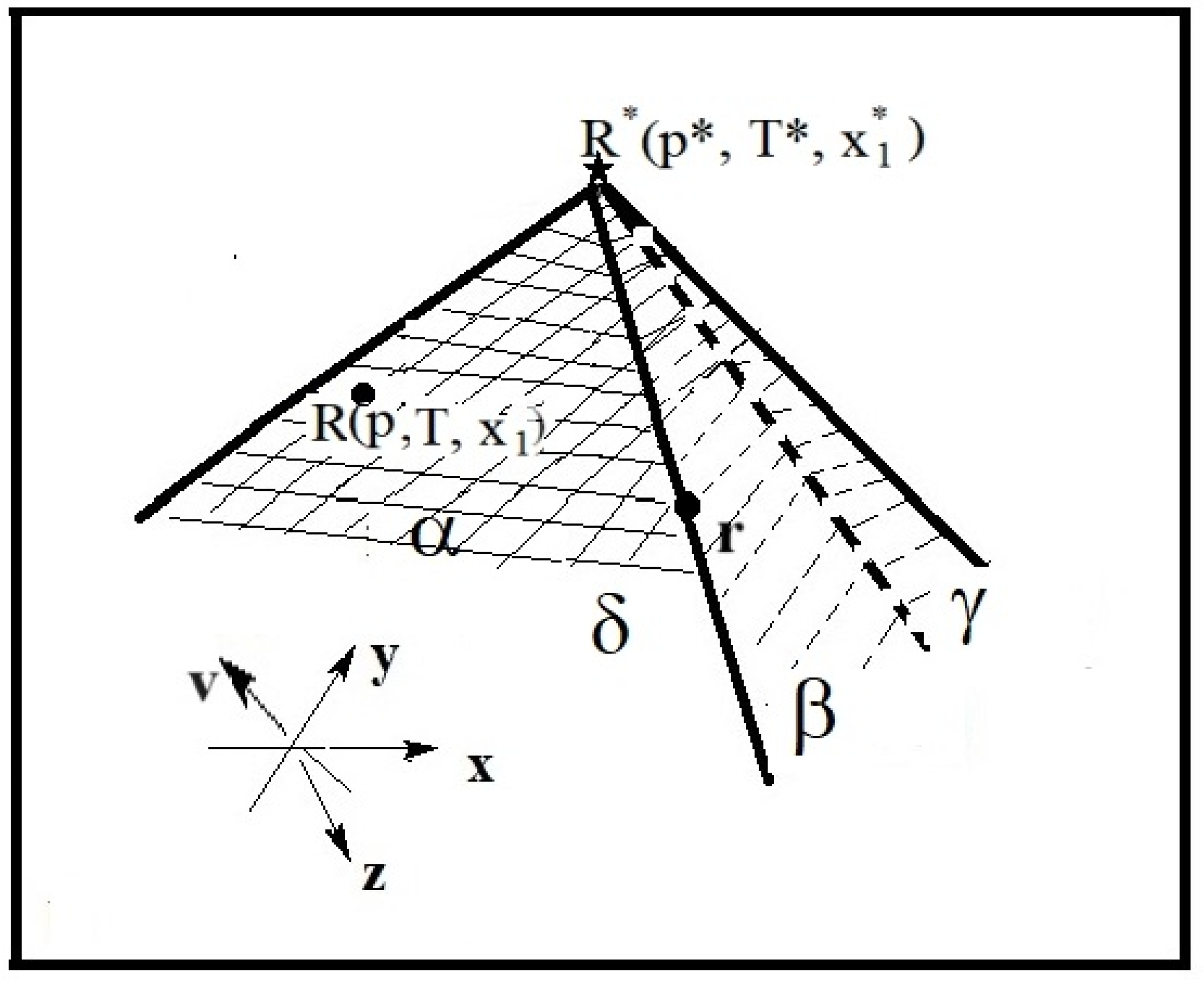
Figure 2.
Topological representation of equilibrium states. Points R1, R2, R3,… etc., resulting from the projection of the classical equilibrium state R onto the invariant state R*, participate in the creation of this representation. These points will constitute the vertices of the state graph. The figure shows a model ternary system.
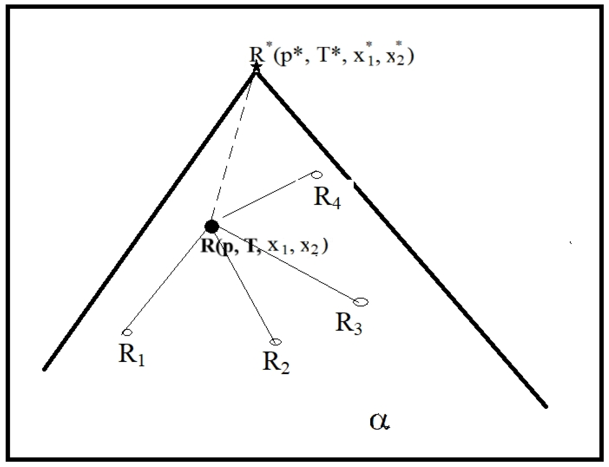
Figure 3.
Topological representation of equilibrium states. Edges connecting individual vertices participate in the creation of this representation. The figure shows a model ternary system.
Figure 3.
Topological representation of equilibrium states. Edges connecting individual vertices participate in the creation of this representation. The figure shows a model ternary system.
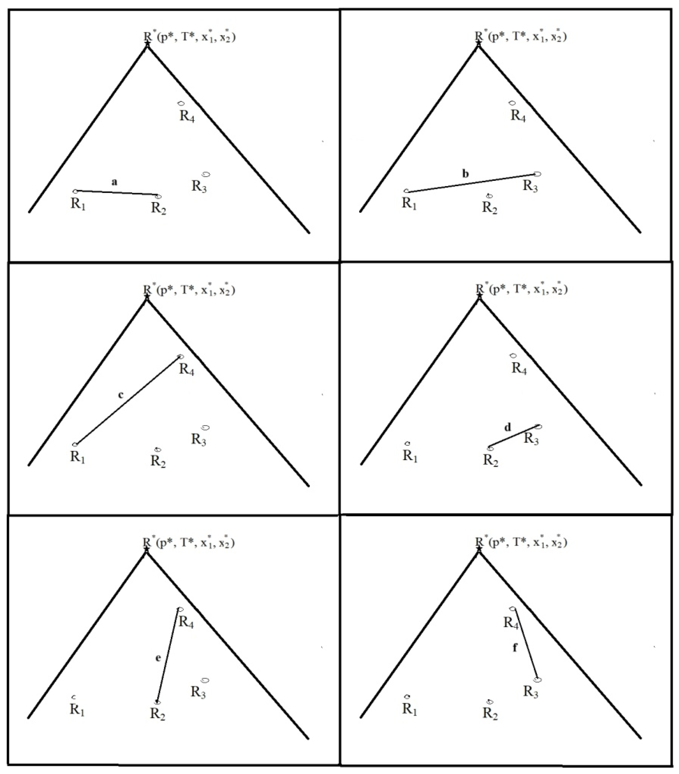
Figure 4.
Topological representation of equilibrium states. This representation is created using paths that are concatenations of edges connecting all vertices. The concatenations thus created represent a graph that is either a linear tree or a branched tree. The path(s) with the shortest length is/are the topological representation of thermodynamic equilibrium. The type of equilibrium state graph determines the type of equilibrium. The figure shows trees corresponding to individual paths. The figure shows a model ternary system.
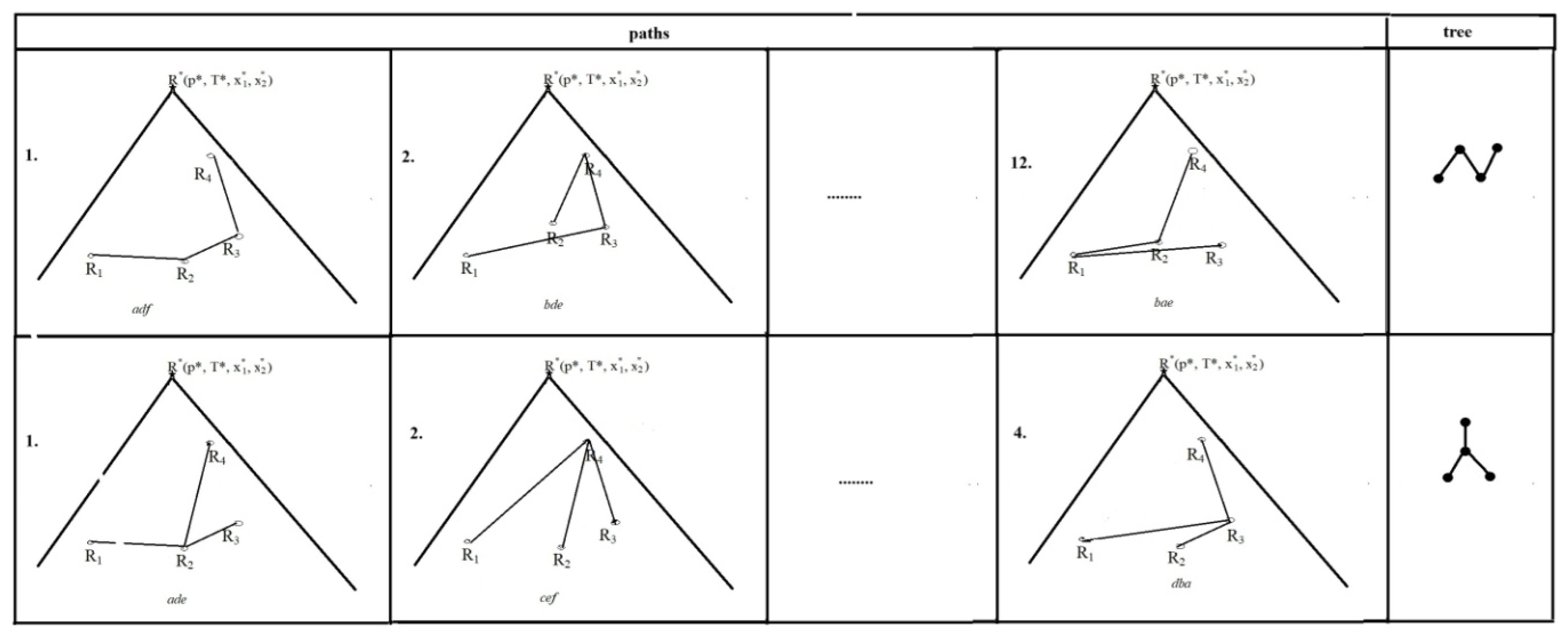
Figure 5.
Topological representation of equilibrium states. This representation allows us to determine the fraction of equilibria of a given type in the total number of all equilibria of the system under consideration. The figure shows, for three-component and four-component systems, what proportion of all single-phase equilibria are equilibria described by a linear tree and branched trees ρ(paths). The figure also demonstrates the forms of state trees and indicates how many paths are represented by a given form of state tree.
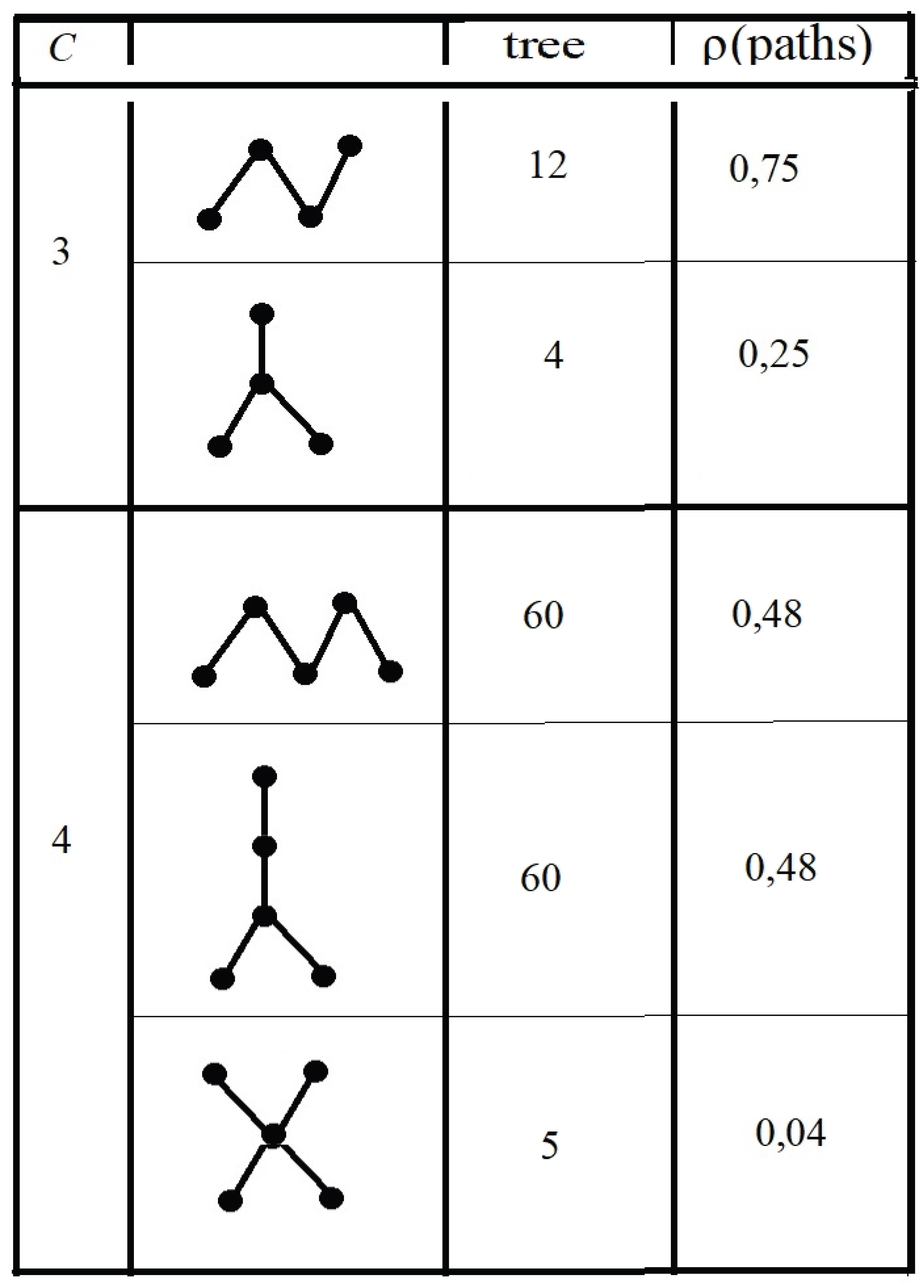
Table 1.
The length of individual edges, eij , of trees lying on a surface isomorphic to a 2-D plane. The edges connect 2 of the 4 points in Nconfig = 51 randomly determined configurations consisting of four points. The maximum length of any edge, eij , does not exceed 10. The lengths eij , are given to 3 decimal places.
| e12 | e13 | e14 | e23 | e24 | e34 | |
|---|---|---|---|---|---|---|
| Nconfig | a | b | c | d | e | f |
| 1 | 8,495 | 9,584 | 8,626 | 5,896 | 6,399 | 9,457 |
| 2 | 9,059 | 5,210 | 6,724 | 9,910 | 7,472 | 6,784 |
| 3 | 3,972 | 5,446 | 2,515 | 7,032 | 2,039 | 2,345 |
| 4 | 7,975 | 1,529 | 7,154 | 3,389 | 4,089 | 8,621 |
| 5 | 6,835 | 5,259 | 6,982 | 6,583 | 7,957 | 6,635 |
| 6 | 6,606 | 5,709 | 7,012 | 2,446 | 1,053 | 9,792 |
| 7 | 0,473 | 1,034 | 5,922 | 2,720 | 8,684 | 1,491 |
| 8 | 4,820 | 2,527 | 4,165 | 6,615 | 4,981 | 1,968 |
| 9 | 8,978 | 6,939 | 0,897 | 2,555 | 6,956 | 8,670 |
| 10 | 4,605 | 1,686 | 0,826 | 9,083 | 3,120 | 4,469 |
| 11 | 3,913 | 6,117 | 9,386 | 5,401 | 2,362 | 5,011 |
| 12 | 0,145 | 0,513 | 8,083 | 2,266 | 9,813 | 9,962 |
| 13 | 9,048 | 4,367 | 3,951 | 9,075 | 9,439 | 4,093 |
| 14 | 6,974 | 5,006 | 1,969 | 7,249 | 1,971 | 7,181 |
| 15 | 5,745 | 4,354 | 2,775 | 7,904 | 2,560 | 6,847 |
| 16 | 2,324 | 2,151 | 4,597 | 1,489 | 2,398 | 8,558 |
| 17 | 8,721 | 0,794 | 5,515 | 9,116 | 9,238 | 1,046 |
| 18 | 2,734 | 4,219 | 3,544 | 0,074 | 8,393 | 5,809 |
| 19 | 8,215 | 3,106 | 9,431 | 4,163 | 6,450 | 1,576 |
| 20 | 0,873 | 2,418 | 5,860 | 6,499 | 7,015 | 3,172 |
| 21 | 6,320 | 8,715 | 9,481 | 5,154 | 8,032 | 2,684 |
| 22 | 5,165 | 4,200 | 3,772 | 6,303 | 4,085 | 1,134 |
| 23 | 4,161 | 9,855 | 7,346 | 8,615 | 9,582 | 9,961 |
| 24 | 0,619 | 0,764 | 9,751 | 2,274 | 2,689 | 6,806 |
| 25 | 6,273 | 2,302 | 0,042 | 4,964 | 7,721 | 6,629 |
| 26 | 1,607 | 2,905 | 9,602 | 5,765 | 3,744 | 1,377 |
| 27 | 9,913 | 1,058 | 8,514 | 0,808 | 8,403 | 4,903 |
| 28 | 9,696 | 9,201 | 0,751 | 2,981 | 8,013 | 8,764 |
| 29 | 7,264 | 3,054 | 7,113 | 8,621 | 5,030 | 6,603 |
| 30 | 7,455 | 3,296 | 8,827 | 5,576 | 9,683 | 2,228 |
| 31 | 8,823 | 2,901 | 9,204 | 0,751 | 5,085 | 4,518 |
| 32 | 0,778 | 4,992 | 7,627 | 8,701 | 3,966 | 3,740 |
| 33 | 4,997 | 6,543 | 4,873 | 8,822 | 0,556 | 5,085 |
| 34 | 0,817 | 4,412 | 3,985 | 9,664 | 1,009 | 5,414 |
| 35 | 3,767 | 9,333 | 1,588 | 6,026 | 7,981 | 9,800 |
| 36 | 2,088 | 7,828 | 5,981 | 0,796 | 6,502 | 8,842 |
| 37 | 6,197 | 1,558 | 6,697 | 0,021 | 5,887 | 6,028 |
| 38 | 2,754 | 8,491 | 7,370 | 7,870 | 7,251 | 4,412 |
| 39 | 9,179 | 3,963 | 8,801 | 9,602 | 1,378 | 4,947 |
| 40 | 1,387 | 6,175 | 6,459 | 0,361 | 4,290 | 0,485 |
| 41 | 9,988 | 2,771 | 9,949 | 3,149 | 2,308 | 9,564 |
| 42 | 8,839 | 4,843 | 0,275 | 6,015 | 3,164 | 2,451 |
| 43 | 6,401 | 3,837 | 2,405 | 5,264 | 3,072 | 1,825 |
| 44 | 2,763 | 8,667 | 5,582 | 1,357 | 8,922 | 8,288 |
| 45 | 0,736 | 0,263 | 3,874 | 2,783 | 4,422 | 8,026 |
| 46 | 5,970 | 1,554 | 5,033 | 8,173 | 1,763 | 1,477 |
| 47 | 0,870 | 9,649 | 1,271 | 2,413 | 8,801 | 4,636 |
| 48 | 2,513 | 5,905 | 7,871 | 3,547 | 0,596 | 0,497 |
| 49 | 1,436 | 1,668 | 4,739 | 0,422 | 3,301 | 0,652 |
| 50 | 6,305 | 6,433 | 6,344 | 1,148 | 8,425 | 5,341 |
| 51 | 9,810 | 2,044 | 4,844 | 3,225 | 0,143 | 4,286 |
Table 2.
The length of individual edges, eij , of trees lying on a surface isomorphic to a 2-D plane. The edges connect 2 of the 4 points in Nconfig = 51 randomly determined configurations consisting of four points. The maximum length of any edge, eij , does not exceed 10. The lengths eij , are given to 3 decimal places.
| e12 | e13 | e14 | e23 | e24 | e34 | |
| Nconfig | a | b | c | d | e | f |
| 1 | 3,237 | 23,858 | 1,205 | 9,293 | 29,059 | 6,580 |
| 2 | 18,349 | 17,979 | 27,398 | 7,561 | 7,425 | 16,087 |
| 3 | 22,898 | 26,571 | 8,144 | 25,995 | 14,506 | 20,086 |
| 4 | 3,773 | 26,506 | 2,951 | 21,640 | 29,188 | 27,448 |
| 5 | 1,543 | 20,330 | 4,747 | 15,475 | 5,025 | 18,806 |
| 6 | 24,799 | 10,374 | 15,747 | 11,329 | 14,710 | 21,777 |
| 7 | 27,059 | 21,951 | 27,911 | 0,313 | 4,141 | 17,864 |
| 8 | 28,842 | 6,930 | 19,028 | 1,601 | 8,621 | 16,917 |
| 9 | 11,003 | 25,372 | 28,707 | 6,675 | 1,939 | 10,852 |
| 10 | 19,212 | 0,589 | 8,992 | 27,522 | 9,067 | 10,197 |
| 11 | 11,110 | 17,080 | 5,099 | 5,531 | 11,997 | 8,589 |
| 12 | 0,937 | 15,245 | 7,624 | 5,953 | 1,014 | 13,033 |
| 13 | 7,351 | 27,930 | 12,417 | 18,251 | 2,281 | 3,841 |
| 14 | 9,740 | 24,351 | 28,557 | 1,549 | 21,921 | 22,857 |
| 15 | 5,521 | 10,367 | 18,649 | 1,323 | 11,729 | 7,068 |
| 16 | 19,937 | 15,358 | 27,935 | 16,988 | 6,243 | 24,650 |
| 17 | 25,167 | 6,984 | 5,700 | 11,055 | 14,367 | 8,442 |
| 18 | 18,619 | 29,874 | 0,543 | 15,797 | 9,049 | 2,887 |
| 19 | 3,282 | 1,772 | 8,834 | 7,016 | 28,832 | 7,283 |
| 20 | 12,645 | 29,002 | 4,381 | 20,578 | 27,453 | 25,286 |
| 21 | 7,887 | 24,092 | 29,975 | 23,301 | 27,486 | 21,006 |
| 22 | 29,811 | 16,969 | 7,632 | 24,307 | 28,362 | 4,536 |
| 23 | 2,890 | 12,452 | 4,024 | 3,631 | 27,440 | 24,735 |
| 24 | 26,301 | 14,792 | 22,119 | 19,371 | 1,136 | 6,001 |
| 25 | 27,746 | 28,625 | 12,645 | 27,825 | 28,468 | 16,606 |
| 26 | 7,622 | 8,803 | 0,145 | 27,934 | 26,396 | 7,151 |
| 27 | 0,326 | 13,818 | 14,125 | 17,791 | 3,636 | 4,251 |
| 28 | 5,733 | 26,057 | 20,058 | 7,050 | 8,326 | 19,733 |
| 29 | 6,732 | 20,007 | 29,027 | 13,730 | 9,969 | 18,024 |
| 30 | 16,257 | 2,851 | 20,990 | 15,308 | 16,796 | 18,186 |
| 31 | 23,882 | 13,257 | 23,183 | 12,365 | 25,891 | 2,299 |
| 32 | 11,287 | 1,657 | 16,584 | 22,851 | 20,709 | 15,062 |
| 33 | 26,997 | 27,735 | 27,957 | 6,249 | 0,225 | 23,574 |
| 34 | 24,188 | 1,308 | 25,298 | 27,456 | 29,341 | 26,245 |
| 35 | 5,625 | 11,749 | 18,398 | 0,685 | 7,554 | 1,308 |
| 36 | 10,191 | 15,835 | 19,142 | 4,713 | 0,741 | 1,081 |
| 37 | 17,569 | 20,188 | 1,288 | 11,525 | 27,969 | 17,409 |
| 38 | 17,837 | 22,841 | 8,723 | 9,791 | 12,038 | 9,252 |
| 39 | 18,244 | 23,162 | 24,044 | 29,399 | 10,936 | 5,194 |
| 40 | 24,871 | 28,268 | 10,779 | 20,936 | 26,120 | 0,763 |
| 41 | 27,687 | 11,651 | 9,697 | 19,749 | 13,619 | 17,408 |
| 42 | 11,522 | 8,678 | 26,749 | 0,053 | 26,971 | 13,498 |
| 43 | 12,108 | 14,624 | 11,460 | 4,970 | 16,754 | 17,201 |
| 44 | 7,092 | 26,077 | 10,794 | 29,001 | 7,143 | 7,907 |
| 45 | 6,151 | 10,844 | 7,035 | 20,677 | 1,671 | 20,843 |
| 46 | 19,550 | 16,604 | 4,604 | 8,901 | 28,808 | 6,458 |
| 47 | 18,723 | 3,333 | 18,748 | 28,096 | 16,526 | 4,023 |
| 48 | 28,088 | 20,175 | 23,792 | 17,079 | 7,388 | 10,466 |
| 49 | 21,092 | 4,074 | 20,517 | 21,623 | 6,354 | 10,832 |
| 50 | 0,803 | 0,140 | 7,352 | 23,459 | 9,949 | 13,042 |
| 51 | 19,865 | 16,096 | 0,840 | 18,225 | 14,101 | 6,969 |
Table 3.
The lengths of paths connecting 4 randomly selected points lying on a 2-D plane (see Table 1). The lengths are normalized to the length of the minimum path. The paths are concatenations of selected 3 edges (a, b, c, ...) from Table 1. Individual edges connect 2 of the 4 points. Paths of minimum length are marked in red. Paths whose length differs negligibly (see equation 30) from the minimum length are shaded in gray. The lengths of the paths are given to 3 decimal places.
| Nconfig | adf | bde | aef | bfe | ced | cfd | abf | acf | ecb | dbc | dac | bae | ade | cef | abc | dbf |
|---|---|---|---|---|---|---|---|---|---|---|---|---|---|---|---|---|
| 1 | 1,147 | 1,052 | 1,171 | 1,224 | 1,006 | 1,153 | 1,324 | 1,278 | 1,184 | 1,159 | 1,107 | 1,177 | 1,000 | 1,178 | 1,284 | 1,199 |
| 2 | 1,327 | 1,164 | 1,201 | 1,003 | 1,242 | 1,207 | 1,085 | 1,163 | 1,000 | 1,126 | 1,324 | 1,120 | 1,363 | 1,081 | 1,082 | 1,129 |
| 3 | 1,935 | 2,104 | 1,211 | 1,425 | 1,679 | 1,724 | 1,705 | 1,280 | 1,450 | 2,173 | 1,960 | 1,661 | 1,891 | 1,000 | 1,730 | 2,149 |
| 4 | 2,219 | 1,000 | 2,297 | 1,581 | 1,625 | 2,128 | 2,012 | 2,637 | 1,418 | 1,340 | 2,056 | 1,509 | 1,716 | 2,206 | 1,850 | 1,503 |
| 5 | 1,085 | 1,072 | 1,160 | 1,074 | 1,165 | 1,093 | 1,014 | 1,107 | 1,093 | 1,019 | 1,104 | 1,085 | 1,157 | 1,168 | 1,032 | 1,000 |
| 6 | 2,047 | 1,000 | 1,895 | 1,798 | 1,142 | 2,091 | 2,401 | 2,543 | 1,496 | 1,647 | 1,745 | 1,452 | 1,098 | 1,939 | 2,099 | 1,949 |
| 7 | 1,562 | 4,148 | 3,551 | 3,738 | 5,778 | 3,379 | 1,000 | 2,630 | 5,216 | 3,227 | 3,040 | 3,399 | 3,961 | 5,368 | 2,478 | 1,749 |
| 8 | 1,439 | 1,516 | 1,264 | 1,017 | 1,692 | 1,369 | 1,000 | 1,176 | 1,253 | 1,429 | 1,675 | 1,324 | 1,763 | 1,193 | 1,236 | 1,193 |
| 9 | 1,944 | 1,583 | 2,368 | 2,172 | 1,002 | 1,167 | 2,366 | 1,785 | 1,424 | 1,000 | 1,196 | 2,201 | 1,779 | 1,590 | 1,618 | 1,748 |
| 10 | 3,224 | 2,466 | 2,165 | 1,647 | 2,313 | 2,553 | 1,911 | 1,758 | 1,000 | 2,059 | 2,577 | 1,671 | 2,984 | 1,494 | 1,264 | 2,706 |
| 11 | 1,269 | 1,230 | 1,000 | 1,195 | 1,519 | 1,754 | 1,333 | 1,622 | 1,583 | 1,852 | 1,657 | 1,098 | 1,035 | 1,485 | 1,720 | 1,465 |
| 12 | 1,416 | 1,441 | 2,279 | 2,321 | 2,307 | 2,324 | 1,215 | 2,081 | 2,106 | 1,243 | 1,201 | 1,198 | 1,398 | 3,187 | 1,000 | 1,458 |
| 13 | 1,300 | 1,339 | 1,321 | 1,047 | 1,314 | 1,002 | 1,024 | 1,000 | 1,039 | 1,018 | 1,291 | 1,337 | 1,612 | 1,023 | 1,016 | 1,026 |
| 14 | 2,393 | 1,590 | 1,803 | 1,583 | 1,251 | 1,833 | 2,142 | 1,802 | 1,000 | 1,590 | 1,810 | 1,560 | 1,810 | 1,243 | 1,559 | 2,173 |
| 15 | 2,115 | 1,529 | 1,564 | 1,420 | 1,366 | 1,809 | 1,749 | 1,586 | 1,000 | 1,551 | 1,695 | 1,306 | 1,673 | 1,257 | 1,329 | 1,972 |
| 16 | 2,049 | 1,000 | 2,200 | 2,171 | 1,405 | 2,425 | 2,159 | 2,564 | 1,515 | 1,364 | 1,393 | 1,138 | 1,029 | 2,576 | 1,503 | 2,020 |
| 17 | 1,788 | 1,813 | 1,800 | 1,049 | 2,260 | 1,484 | 1,000 | 1,447 | 1,472 | 1,461 | 2,211 | 1,776 | 2,564 | 1,496 | 1,423 | 1,037 |
| 18 | 1,357 | 1,997 | 2,666 | 2,900 | 1,891 | 1,484 | 2,009 | 1,903 | 2,543 | 1,234 | 1,000 | 2,416 | 1,763 | 2,794 | 1,653 | 1,590 |
| 19 | 1,578 | 1,551 | 1,836 | 1,259 | 2,266 | 1,715 | 1,458 | 2,173 | 2,147 | 1,888 | 2,466 | 2,009 | 2,129 | 1,974 | 2,346 | 1,000 |
| 20 | 1,631 | 2,465 | 1,711 | 1,950 | 2,997 | 2,403 | 1,000 | 1,532 | 2,366 | 2,286 | 2,047 | 1,595 | 2,226 | 2,483 | 1,416 | 1,870 |
| 21 | 1,000 | 1,547 | 1,203 | 1,372 | 1,601 | 1,223 | 1,252 | 1,306 | 1,853 | 1,649 | 1,480 | 1,629 | 1,378 | 1,427 | 1,732 | 1,169 |
| 22 | 1,402 | 1,622 | 1,155 | 1,048 | 1,575 | 1,247 | 1,168 | 1,120 | 1,341 | 1,588 | 1,695 | 1,496 | 1,730 | 1,000 | 1,461 | 1,294 |
| 23 | 1,130 | 1,394 | 1,178 | 1,461 | 1,269 | 1,288 | 1,192 | 1,067 | 1,331 | 1,283 | 1,000 | 1,173 | 1,111 | 1,336 | 1,062 | 1,413 |
| 24 | 2,382 | 1,407 | 2,484 | 2,520 | 3,614 | 4,625 | 2,011 | 4,218 | 3,243 | 3,141 | 3,105 | 1,000 | 1,371 | 4,727 | 2,734 | 2,418 |
| 25 | 2,445 | 2,051 | 2,822 | 2,279 | 1,741 | 1,592 | 2,080 | 1,771 | 1,377 | 1,000 | 1,543 | 2,230 | 2,594 | 1,969 | 1,179 | 1,901 |
| 26 | 1,486 | 2,108 | 1,142 | 1,363 | 3,245 | 2,843 | 1,000 | 2,137 | 2,760 | 3,103 | 2,882 | 1,402 | 1,887 | 2,500 | 2,397 | 1,706 |
| 27 | 2,308 | 1,517 | 3,430 | 2,122 | 2,618 | 2,101 | 2,345 | 3,447 | 2,655 | 1,533 | 2,842 | 2,862 | 2,825 | 3,223 | 2,879 | 1,000 |
| 28 | 1,826 | 1,720 | 2,254 | 2,212 | 1,000 | 1,064 | 2,355 | 1,636 | 1,530 | 1,101 | 1,143 | 2,291 | 1,762 | 1,492 | 1,673 | 1,783 |
| 29 | 1,531 | 1,137 | 1,287 | 1,000 | 1,414 | 1,521 | 1,152 | 1,428 | 1,035 | 1,279 | 1,566 | 1,045 | 1,424 | 1,276 | 1,187 | 1,245 |
| 30 | 1,375 | 1,672 | 1,745 | 1,370 | 2,170 | 1,498 | 1,169 | 1,668 | 1,964 | 1,594 | 1,969 | 1,841 | 2,046 | 1,868 | 1,764 | 1,000 |
| 31 | 1,725 | 1,069 | 2,255 | 1,530 | 1,841 | 1,771 | 1,988 | 2,759 | 2,104 | 1,574 | 2,298 | 2,057 | 1,794 | 2,302 | 2,562 | 1,000 |
| 32 | 1,558 | 2,081 | 1,000 | 1,497 | 2,392 | 2,365 | 1,121 | 1,432 | 1,955 | 2,513 | 2,016 | 1,148 | 1,585 | 1,807 | 1,579 | 2,055 |
| 33 | 1,798 | 1,514 | 1,012 | 1,159 | 1,355 | 1,786 | 1,581 | 1,422 | 1,139 | 1,925 | 1,778 | 1,150 | 1,367 | 1,000 | 1,561 | 1,945 |
| 34 | 2,548 | 2,418 | 1,161 | 1,737 | 2,350 | 3,056 | 1,706 | 1,638 | 1,508 | 2,895 | 2,319 | 1,000 | 1,842 | 1,668 | 1,477 | 3,124 |
| 35 | 1,722 | 2,051 | 1,893 | 2,382 | 1,370 | 1,530 | 2,012 | 1,332 | 1,661 | 1,489 | 1,000 | 1,852 | 1,562 | 1,702 | 1,291 | 2,211 |
| 36 | 1,323 | 1,706 | 1,966 | 2,614 | 1,498 | 1,762 | 2,116 | 1,908 | 2,291 | 1,648 | 1,000 | 1,852 | 1,059 | 2,406 | 1,793 | 1,970 |
| 37 | 1,640 | 1,000 | 2,426 | 1,805 | 1,688 | 1,707 | 1,846 | 2,534 | 1,894 | 1,108 | 1,730 | 1,827 | 1,621 | 2,493 | 1,936 | 1,019 |
| 38 | 1,043 | 1,638 | 1,000 | 1,398 | 1,560 | 1,363 | 1,086 | 1,008 | 1,603 | 1,646 | 1,248 | 1,283 | 1,240 | 1,320 | 1,291 | 1,441 |
| 39 | 2,306 | 1,452 | 1,507 | 1,000 | 1,923 | 2,269 | 1,758 | 2,228 | 1,374 | 2,174 | 2,681 | 1,411 | 1,959 | 1,470 | 2,133 | 1,799 |
| 40 | 1,000 | 4,848 | 2,759 | 4,903 | 4,976 | 3,271 | 3,603 | 3,731 | 7,579 | 5,820 | 3,676 | 5,308 | 2,704 | 5,031 | 6,279 | 3,144 |
| 41 | 2,759 | 1,000 | 2,657 | 1,780 | 1,872 | 2,754 | 2,713 | 3,586 | 1,827 | 1,929 | 2,806 | 1,831 | 1,877 | 2,652 | 2,760 | 1,882 |
| 42 | 2,938 | 2,381 | 2,454 | 1,776 | 1,605 | 1,484 | 2,739 | 1,964 | 1,406 | 1,890 | 2,569 | 2,860 | 3,059 | 1,000 | 2,370 | 2,260 |
| 43 | 1,848 | 1,667 | 1,547 | 1,196 | 1,471 | 1,300 | 1,652 | 1,456 | 1,276 | 1,576 | 1,927 | 1,823 | 2,018 | 1,000 | 1,732 | 1,496 |
| 44 | 1,279 | 1,953 | 2,059 | 2,667 | 1,635 | 1,570 | 2,032 | 1,714 | 2,388 | 1,609 | 1,000 | 2,098 | 1,344 | 2,349 | 1,753 | 1,887 |
| 45 | 2,369 | 1,533 | 2,706 | 2,609 | 2,274 | 3,013 | 1,852 | 2,593 | 1,756 | 1,420 | 1,517 | 1,113 | 1,630 | 3,350 | 1,000 | 2,272 |
| 46 | 3,258 | 2,397 | 1,921 | 1,000 | 3,122 | 3,063 | 1,878 | 2,603 | 1,742 | 3,079 | 4,000 | 1,937 | 3,318 | 1,726 | 2,619 | 2,337 |
| 47 | 1,739 | 4,582 | 3,142 | 5,070 | 2,742 | 1,827 | 3,328 | 1,488 | 4,331 | 2,928 | 1,000 | 4,243 | 2,654 | 3,230 | 2,589 | 3,667 |
| 48 | 1,818 | 2,786 | 1,000 | 1,941 | 3,331 | 3,304 | 2,472 | 3,017 | 3,985 | 4,803 | 3,863 | 2,499 | 1,846 | 2,486 | 4,517 | 2,759 |
| 49 | 1,000 | 2,148 | 2,147 | 2,239 | 3,371 | 2,316 | 1,497 | 2,720 | 3,868 | 2,721 | 2,629 | 2,552 | 2,055 | 3,463 | 3,125 | 1,093 |
| 50 | 1,000 | 1,251 | 1,569 | 1,579 | 1,244 | 1,003 | 1,413 | 1,406 | 1,657 | 1,088 | 1,078 | 1,654 | 1,241 | 1,572 | 1,491 | 1,010 |
| 51 | 3,201 | 1,000 | 2,631 | 1,196 | 1,517 | 2,283 | 2,982 | 3,500 | 1,299 | 1,869 | 3,304 | 2,217 | 2,435 | 1,714 | 3,085 | 1,766 |
Table 4.
The lengths of paths connecting 4 randomly selected points lying on a 2-D plane (see Table 2). The lengths are normalized to the length of the minimum path. The paths are concatenations of selected 3 edges (a, b, c, ...) from Table 1. Individual edges connect 2 of the 4 points. Paths of minimum length are marked in red. Paths whose length differs negligibly (see equation 30) from the minimum length are shaded in gray. The lengths of the paths are given to 3 decimal places.
| Nconfig | adf | bde | aef | bfe | ced | cfd | abf | acf | ecb | dbc | dac | bae | ade | cef | abc | dbf |
|---|---|---|---|---|---|---|---|---|---|---|---|---|---|---|---|---|
| 1 | 1,734 | 5,644 | 3,527 | 5,398 | 3,589 | 1,549 | 3,055 | 1,000 | 4,910 | 3,117 | 1,246 | 5,095 | 3,773 | 3,343 | 2,568 | 3,605 |
| 2 | 1,274 | 1,000 | 1,270 | 1,259 | 1,286 | 1,548 | 1,590 | 1,876 | 1,602 | 1,606 | 1,617 | 1,327 | 1,011 | 1,544 | 1,933 | 1,263 |
| 3 | 1,614 | 1,569 | 1,345 | 1,431 | 1,138 | 1,269 | 1,628 | 1,196 | 1,152 | 1,421 | 1,335 | 1,497 | 1,484 | 1,000 | 1,348 | 1,700 |
| 4 | 1,864 | 2,727 | 2,130 | 2,931 | 1,896 | 1,835 | 2,035 | 1,205 | 2,068 | 1,801 | 1,000 | 2,097 | 1,925 | 2,101 | 1,172 | 2,665 |
| 5 | 1,646 | 1,876 | 1,166 | 2,029 | 1,160 | 1,793 | 1,869 | 1,153 | 1,383 | 1,863 | 1,000 | 1,236 | 1,013 | 1,313 | 1,223 | 2,509 |
| 6 | 1,590 | 1,000 | 1,683 | 1,287 | 1,148 | 1,342 | 1,564 | 1,712 | 1,121 | 1,028 | 1,425 | 1,370 | 1,396 | 1,434 | 1,398 | 1,194 |
| 7 | 1,713 | 1,000 | 1,858 | 1,665 | 1,226 | 1,745 | 2,533 | 2,758 | 2,045 | 1,900 | 2,094 | 2,013 | 1,193 | 1,890 | 2,913 | 1,520 |
| 8 | 2,761 | 1,000 | 3,171 | 1,893 | 1,705 | 2,189 | 3,072 | 3,777 | 2,016 | 1,607 | 2,884 | 2,588 | 2,278 | 2,598 | 3,195 | 1,484 |
| 9 | 1,454 | 1,732 | 1,213 | 1,945 | 1,902 | 2,357 | 2,407 | 2,577 | 2,855 | 3,097 | 2,364 | 1,953 | 1,000 | 2,115 | 3,317 | 2,187 |
| 0 | 3,053 | 1,994 | 2,063 | 1,065 | 2,444 | 2,505 | 1,609 | 2,059 | 1,000 | 1,990 | 2,988 | 1,548 | 2,992 | 1,515 | 1,544 | 2,054 |
| 1 | 1,313 | 1,801 | 1,649 | 1,960 | 1,177 | 1,000 | 1,914 | 1,290 | 1,778 | 1,442 | 1,131 | 2,091 | 1,490 | 1,336 | 1,732 | 1,623 |
| 2 | 2,521 | 2,810 | 1,896 | 3,706 | 1,846 | 3,367 | 3,697 | 2,732 | 3,022 | 3,647 | 1,836 | 2,176 | 1,000 | 2,742 | 3,012 | 4,331 |
| 13 | 2,185 | 3,597 | 1,000 | 2,527 | 2,445 | 2,561 | 2,904 | 1,752 | 3,164 | 4,349 | 2,822 | 2,788 | 2,069 | 1,376 | 3,540 | 3,713 |
| 14 | 1,028 | 1,440 | 1,642 | 2,082 | 1,567 | 1,595 | 1,715 | 1,841 | 2,253 | 1,640 | 1,200 | 1,687 | 1,000 | 2,208 | 1,886 | 1,468 |
| 15 | 1,000 | 1,683 | 1,748 | 2,096 | 2,279 | 1,944 | 1,650 | 2,245 | 2,929 | 2,181 | 1,832 | 1,985 | 1,335 | 2,692 | 2,483 | 1,348 |
| 16 | 1,596 | 1,000 | 1,317 | 1,199 | 1,326 | 1,803 | 1,553 | 1,879 | 1,284 | 1,562 | 1,681 | 1,076 | 1,119 | 1,524 | 1,639 | 1,477 |
| 17 | 1,881 | 1,365 | 2,021 | 1,255 | 1,311 | 1,061 | 1,710 | 1,656 | 1,140 | 1,000 | 1,766 | 1,960 | 2,131 | 1,201 | 1,594 | 1,115 |
| 18 | 2,989 | 4,385 | 2,448 | 3,350 | 2,034 | 1,541 | 4,117 | 1,767 | 3,162 | 3,703 | 2,801 | 4,611 | 3,483 | 1,000 | 3,929 | 3,891 |
| 19 | 1,425 | 3,049 | 3,193 | 3,071 | 3,622 | 1,875 | 1,000 | 1,572 | 3,197 | 1,428 | 1,551 | 2,747 | 3,172 | 3,643 | 1,126 | 1,303 |
| 20 | 1,556 | 2,049 | 1,739 | 2,174 | 1,394 | 1,336 | 1,780 | 1,125 | 1,618 | 1,435 | 1,000 | 1,838 | 1,614 | 1,519 | 1,224 | 1,991 |
| 21 | 1,000 | 1,435 | 1,080 | 1,391 | 1,547 | 1,423 | 1,015 | 1,128 | 1,562 | 1,482 | 1,172 | 1,139 | 1,124 | 1,503 | 1,187 | 1,310 |
| 22 | 1,608 | 1,909 | 1,719 | 1,367 | 1,653 | 1,000 | 1,407 | 1,151 | 1,452 | 1,341 | 1,693 | 2,060 | 2,261 | 1,111 | 1,492 | 1,256 |
| 23 | 2,964 | 4,127 | 5,222 | 6,128 | 3,328 | 3,071 | 3,800 | 3,001 | 4,164 | 1,907 | 1,000 | 4,057 | 3,220 | 5,329 | 1,836 | 3,871 |
| 24 | 2,356 | 1,610 | 1,525 | 1,000 | 1,944 | 2,166 | 2,148 | 2,482 | 1,735 | 2,567 | 3,091 | 1,926 | 2,135 | 1,334 | 2,883 | 1,832 |
| 25 | 1,266 | 1,490 | 1,278 | 1,293 | 1,209 | 1,001 | 1,280 | 1,000 | 1,224 | 1,212 | 1,197 | 1,488 | 1,474 | 1,013 | 1,211 | 1,282 |
| 26 | 2,863 | 4,232 | 2,760 | 2,839 | 3,652 | 2,362 | 1,580 | 1,000 | 2,369 | 2,472 | 2,393 | 2,870 | 4,153 | 2,258 | 1,111 | 2,942 |
| 27 | 2,723 | 4,291 | 1,000 | 2,643 | 4,329 | 4,404 | 2,240 | 2,277 | 3,845 | 5,568 | 3,926 | 2,165 | 2,649 | 2,680 | 3,442 | 4,366 |
| 28 | 1,540 | 1,963 | 1,601 | 2,564 | 1,679 | 2,219 | 2,441 | 2,157 | 2,579 | 2,519 | 1,556 | 1,900 | 1,000 | 2,280 | 2,456 | 2,503 |
| 29 | 1,265 | 1,436 | 1,141 | 1,577 | 1,733 | 1,997 | 1,471 | 1,767 | 1,939 | 2,062 | 1,626 | 1,206 | 1,000 | 1,874 | 1,833 | 1,701 |
| 30 | 1,423 | 1,000 | 1,466 | 1,082 | 1,519 | 1,559 | 1,067 | 1,586 | 1,163 | 1,120 | 1,504 | 1,027 | 1,384 | 1,601 | 1,147 | 1,040 |
| 31 | 1,381 | 1,845 | 1,865 | 1,484 | 2,200 | 1,355 | 1,413 | 1,768 | 2,232 | 1,748 | 2,128 | 2,257 | 2,225 | 1,840 | 2,160 | 1,000 |
| 32 | 1,757 | 1,615 | 1,680 | 1,336 | 2,148 | 1,946 | 1,000 | 1,533 | 1,391 | 1,467 | 1,811 | 1,202 | 1,958 | 1,869 | 1,054 | 1,413 |
| 33 | 1,698 | 1,022 | 1,518 | 1,540 | 1,029 | 1,726 | 2,340 | 2,346 | 1,671 | 1,851 | 1,829 | 1,642 | 1,000 | 1,546 | 2,470 | 1,720 |
| 34 | 1,533 | 1,144 | 1,571 | 1,120 | 1,616 | 1,555 | 1,019 | 1,491 | 1,101 | 1,064 | 1,515 | 1,080 | 1,594 | 1,592 | 1,000 | 1,083 |
| 35 | 1,000 | 2,624 | 1,902 | 2,706 | 3,497 | 2,677 | 2,453 | 3,325 | 4,950 | 4,048 | 3,244 | 3,273 | 1,820 | 3,579 | 4,696 | 1,804 |
| 36 | 1,331 | 1,772 | 1,000 | 1,470 | 2,047 | 2,076 | 2,256 | 2,532 | 2,973 | 3,304 | 2,834 | 2,228 | 1,302 | 1,745 | 3,760 | 1,801 |
| 37 | 1,539 | 1,975 | 2,083 | 2,169 | 1,349 | 1,000 | 1,825 | 1,200 | 1,636 | 1,092 | 1,005 | 2,175 | 1,888 | 1,544 | 1,292 | 1,625 |
| 38 | 1,328 | 1,609 | 1,409 | 1,589 | 1,100 | 1,000 | 1,798 | 1,290 | 1,570 | 1,489 | 1,309 | 1,899 | 1,429 | 1,081 | 1,779 | 1,508 |
| 39 | 1,537 | 1,847 | 1,000 | 1,143 | 1,873 | 1,706 | 1,356 | 1,381 | 1,691 | 2,229 | 2,085 | 1,523 | 1,704 | 1,169 | 1,904 | 1,680 |
| 40 | 1,434 | 2,319 | 1,593 | 1,698 | 1,781 | 1,000 | 1,660 | 1,121 | 2,006 | 1,847 | 1,742 | 2,440 | 2,215 | 1,160 | 1,968 | 1,538 |
| 41 | 1,854 | 1,287 | 1,679 | 1,221 | 1,232 | 1,340 | 1,623 | 1,567 | 1,000 | 1,175 | 1,634 | 1,515 | 1,746 | 1,165 | 1,402 | 1,396 |
| 42 | 1,128 | 1,606 | 2,339 | 2,211 | 2,419 | 1,813 | 1,516 | 2,329 | 2,807 | 1,596 | 1,724 | 2,122 | 1,734 | 3,024 | 2,112 | 1,000 |
| 43 | 1,201 | 1,274 | 1,614 | 1,702 | 1,163 | 1,178 | 1,539 | 1,429 | 1,501 | 1,088 | 1,000 | 1,524 | 1,186 | 1,591 | 1,338 | 1,289 |
| 44 | 1,987 | 2,810 | 1,000 | 1,857 | 2,120 | 2,154 | 1,855 | 1,165 | 1,988 | 2,975 | 2,118 | 1,821 | 1,953 | 1,167 | 1,985 | 2,845 |
| 45 | 2,554 | 1,778 | 1,536 | 1,787 | 1,574 | 2,601 | 2,027 | 1,823 | 1,047 | 2,066 | 1,814 | 1,000 | 1,527 | 1,583 | 1,287 | 2,805 |
| 46 | 1,749 | 2,721 | 2,746 | 2,598 | 2,120 | 1,000 | 2,135 | 1,533 | 2,505 | 1,508 | 1,656 | 3,254 | 2,868 | 1,997 | 2,042 | 1,601 |
| 47 | 2,129 | 2,008 | 1,644 | 1,000 | 2,654 | 2,130 | 1,092 | 1,737 | 1,617 | 2,101 | 2,746 | 1,616 | 2,652 | 1,645 | 1,709 | 1,484 |
| 48 | 1,463 | 1,174 | 1,208 | 1,000 | 1,269 | 1,350 | 1,544 | 1,639 | 1,350 | 1,605 | 1,813 | 1,463 | 1,382 | 1,095 | 1,895 | 1,255 |
| 49 | 2,519 | 1,508 | 1,800 | 1,000 | 2,281 | 2,492 | 1,693 | 2,467 | 1,456 | 2,174 | 2,974 | 1,483 | 2,308 | 1,773 | 2,149 | 1,718 |
| 50 | 4,497 | 4,044 | 2,868 | 2,788 | 4,913 | 5,286 | 1,686 | 2,555 | 2,102 | 3,731 | 3,811 | 1,313 | 4,124 | 3,658 | 1,000 | 4,417 |
| 51 | 2,057 | 2,210 | 1,868 | 1,696 | 1,514 | 1,188 | 1,959 | 1,263 | 1,417 | 1,605 | 1,777 | 2,285 | 2,382 | 1,000 | 1,680 | 1,885 |
Table 5.
The most important properties of the paths presented in Tables 1–A11. The symbols nlt and nbt denote the number of paths representing linear and branched trees, respectively; ρlt and ρbt - are the probabilities of finding a linear and branched tree among all paths; Ni, i = 1, 2, 3 - is the number of configurations with: one, two, and three or more paths of minimum or near-minimum length, respectively. Nconfig =51.
| 0 < eij < emax | |||||
| emax = | random(1) | random(3) | random(5) | random(10) | random(30) |
| nlt | 40 | 40 | 35 | 38 | 38 |
| nbt | 11 | 11 | 16 | 13 | 13 |
| ρlt | 0,784 | 0,784 | 0,686 | 0,745 | 0,745 |
| ρbt | 0,216 | 0,216 | 0,314 | 0,255 | 0,255 |
| N1 | 39 | 38 | 40 | 38 | 35 |
| N2 | 8 | 11 | 8 | 8 | 9 |
| N3 | 4 | 2 | 3 | 5 | 3 |
Disclaimer/Publisher’s Note: The statements, opinions and data contained in all publications are solely those of the individual author(s) and contributor(s) and not of MDPI and/or the editor(s). MDPI and/or the editor(s) disclaim responsibility for any injury to people or property resulting from any ideas, methods, instructions or products referred to in the content. |
© 2025 by the authors. Licensee MDPI, Basel, Switzerland. This article is an open access article distributed under the terms and conditions of the Creative Commons Attribution (CC BY) license (http://creativecommons.org/licenses/by/4.0/).
Copyright: This open access article is published under a Creative Commons CC BY 4.0 license, which permit the free download, distribution, and reuse, provided that the author and preprint are cited in any reuse.


