An Experimental Determinant Model for Zeta Zeros

1. Introduction and Motivation

The spectral interpretation of zeta zeros has long been considered a plausible route to RH, linking number theory and quantum/spectral ideas (see, e.g., [2], Ch. 1–2] and [1], Ch. 14]). On the physics side, quantum-graph models provide a minimal setting for chaotic scattering and trace formulae [5], while the Hamiltonian viewpoint of Berry and Keating [4] frames zeta zeros as a putative spectrum. Large-scale computations of zeros (heights, spacings, and the success of random-matrix predictions) are surveyed in [3] and set a high bar for any candidate model.

We explore a determinant built from a simple network carrying prime lengths $L_p=logp$. Its scattering determinant separates into an Euler-like product and a coherent rank-1 correction, yielding a line observable that can be compared to the exact smooth backbone derived from the $\Gamma$-factor. Our aim in this note is conceptual and empirical: to specify the model precisely, describe the diagnostics it passes, and report the residuals against large zero sets.

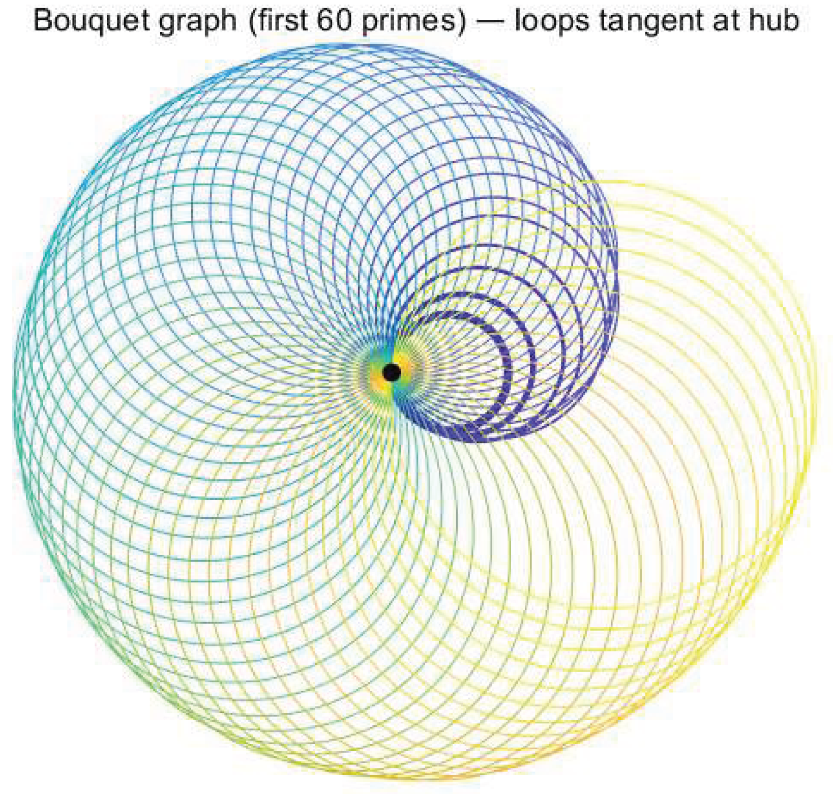
Figure 1. Schematic network used to assemble the determinant.

Figure 1. Schematic network used to assemble the determinant.

2. The Determinant Model and Its Line Observable

2.1. Setup and Hub Mixing

Let $\mathcal{P}$ denote the primes and assign to each $p\in \mathcal{P}$ a loop “time” $L_p=logp$. Work on ${\ell }^2\left(\mathcal{P}\right)$ with a unit vector $u={\left(u_p\right)}_{p\in \mathcal{P}}$,

$$u_p\propto p^{-1/2-{\delta }_u},{\delta }_u>0.$$

(1)

At the hub we impose the rank-1 unitary

$$U(\eta ,\psi )=e^{i\psi }\left(I+\left(e^{2i\eta }-1\right)|u\rangle \langle u|\right),\eta ,\psi \in \mathbb{R},$$

(2)

where $\psi$ is a global phase and $\eta$ controls a single coherent channel. Quantum-graph unitaries of this type are standard scattering couplers [5].

2.2. Diagonal Propagation and Regularization

Along $s=\frac{1}{2}+it$ the exact per-prime propagation is $p^{-s}=e^{-L_p/2}{e}^{-it{L}_p}$. We package this into a diagonal operator

$$D_{\chi ,\Delta }\left(s\right)=\mathrm{diag}\left(\chi \left(p\right)p^{-s}{w}_p\left(s\right)\right),w_p\left(s\right)\in (0,1],$$

(3)

with $\chi$ a Dirichlet character (trivial for $\zeta$). Two practically useful windows:

• Fejér (line) window on $s=\frac{1}{2}+it$: $w_p\left(t\right)=max{\{0,1-{(L_p/\left(c\Delta \left(t\right)\right))}^2\}}^q$ with $\Delta \left(t\right)=\kappa loglog(max\{t,t_{min}\})$. This mimics the explicit-formula cutoff and is numerically robust on the line.
• Analytic Gaussian$w_p\left(s\right)=exp\left(-\tau \left(s\right)L_p^2\right)$ with $\tau$ holomorphic near $\Re s\ge \frac{1}{2}$ (e.g. $\tau \left(s\right)\equiv {\alpha }_0>0$). This favors analytic continuation but is less aggressive than the Fejér taper for finite tables.

For standard properties of $\zeta$ and its $\Gamma$-factor we refer to [1].

2.3. Determinant, Bracket, and Observable

The determinant factorizes as

$$D\left(s\right)=det\left(I-a{D}_{\chi ,\Delta }\left(s\right)\right)·\left(1-b\overline{s}\left(s\right)\right),a=e^{i\psi },b=e^{i\psi }\left(e^{2i\eta }-1\right),$$

(4)

where the rank-1 bracket

$$\overline{s}\left(s\right)=\langle u,{(I-a{D}_{\chi ,\Delta }\left(s\right))}^{-1}{D}_{\chi ,\Delta }\left(s\right)u\rangle$$

(5)

captures the unique coherent channel. On the line we read the oscillatory count

$$S_{det}\left(t\right):=-{\displaystyle \frac{1}{\pi }}\Im logD\left(\frac{1}{2}+it\right).$$

(6)

For comparison we use the exact smooth backbone $N_{\mathrm{sm}}\left(t\right)=\vartheta \left(t\right)/\pi$, with

$${\vartheta }_{\zeta }\left(t\right)=\Im log\Gamma \left(\frac{1}{4}+\frac{it}{2}\right)-\frac{t}{2}log\pi ,{\vartheta }_{\chi }\left(t\right)=\Im log\Gamma \left(\frac{1/2+a+it}{2}\right)+\frac{t}{2}log{\displaystyle \frac{q}{\pi }}.$$

(7)

The bouquet-like separation (4) mirrors Euler product times a low-rank correction; see the general scattering perspective in [5].

Finite-P Diagnostic

For a finite prime set, the matrix determinant lemma yields

$$det\left(I-a{D}_{\chi ,\Delta }\left(s\right)U(\eta ,\psi )\right)=\left(\prod _{p\le P}\left(1-a\chi \left(p\right)p^{-s}{w}_p\left(s\right)\right)\right)·\left(1-b\overline{s}\left(s\right)\right),$$

verified numerically to machine precision in our runs; this supports the stability of (4)–(5).

3. Scoring Against Zeros

Let $t_k$ be the positive ordinates of zeros on the critical line (with multiplicity). We form residuals

$$e_k=\left(N_{\mathrm{sm}}\left(t_k\right)-S_{det}\left(t_k\right)-C_0\right)-k,$$

(8)

calibrating $C_0$ on a short prefix and scoring on the hold-out. We report RMS$\left(e_k\right)$, P95 of $|e_k|$, and $max|e_k|$. This follows standard practice in numerical $\zeta$ studies [3].

Parameters

A single set works across $\zeta$ and a sample Dirichlet family: $\eta \in [0,0.09]$, $\psi \in [0.08,0.095]$, Fejér scale $\kappa \approx 4.4$, and $u_p\propto p^{-1/2-{\delta }_u}$ with ${\delta }_u\approx 0.05$. The analytic Gaussian uses a small ${\alpha }_0$ when we prefer holomorphic regularization.

4. Numerical Experiments

We summarize (i) zeta zeros up to $K=600,000$, and (ii) the first $K=129$ zeros of a real character modulo 5 (even, $a=0$). In both cases we used $8,000$ primes (max $p=81,799$) and exact per-loop unitary propagation.

4.1. Zeta Zeros: Sweep and Full Score

On a $K=150,000$ slice we sweep $(\eta ,\psi ,\kappa )$:

$$(\eta ,\psi ,\kappa )\approx (0.085,0.085,4.40)\Rightarrow \mathrm{RMS}\approx 0.0468\left(\mathrm{slice}\right).$$

Freezing these, the full $K=600,000$ run (calibration $M_{\mathrm{cal}}=1000$) achieves

$$\mathrm{RMS}\approx 0.0546,\mathrm{P}95\approx 0.553,max|e_k|\approx 0.990.$$

By bands: $[1,2·{10}^5]$ RMS $0.0484$, $[2·{10}^5,4·{10}^5]$ RMS $0.0556$, $[4·{10}^5,6·{10}^5]$ RMS $0.0592$. These scales are consistent with the known backbone and the slow variation of the entire factor on $\sigma >1$ [1].

4.2. Dirichlet L (mod 5, Even)

On the first 129 positive zeros we tune $(\eta ,\psi ,\kappa )$ (calibrating $C_0$ on the first 20 zeros) and obtain

$$(\eta ,\psi ,\kappa )\approx (0.080,0.085,4.44)\Rightarrow \mathrm{RMS}\approx 0.0197,$$

with P95 $\approx 0.0280$ and $max\approx 0.1066$ (hold-out $K=109$). The stability under prime depth and modest window jitter suggests the mechanism transfers across families, a desirable feature in any spectral model of $\Lambda \left(s\right)$ [4].

4.3. Summary Table

Table 1. Residual statistics on hold-out sets.

Family	K	Primes	$(\mathit{\eta },\mathit{\psi },\mathit{\kappa })$	RMS	P95	Max
$\zeta$ (full)	$600,000$	8000	$(0.085,0.085,4.40)$	$0.0546$	$0.5529$	$0.9903$
$\zeta$ (slice)	$150,000$	8000	best-of-grid	$0.0468$	—	—
$L({\chi }_5,·)$	129	8000	$(0.080,0.085,4.44)$	$0.0197$	$0.0280$	$0.1066$

Table 1. Residual statistics on hold-out sets.

Family	K	Primes	$(\mathit{\eta },\mathit{\psi },\mathit{\kappa })$	RMS	P95	Max
$\zeta$ (full)	$600,000$	8000	$(0.085,0.085,4.40)$	$0.0546$	$0.5529$	$0.9903$
$\zeta$ (slice)	$150,000$	8000	best-of-grid	$0.0468$	—	—
$L({\chi }_5,·)$	129	8000	$(0.080,0.085,4.44)$	$0.0197$	$0.0280$	$0.1066$

5. Diagnostics and Analytic Design

We implemented diagnostics that mirror the analytic roadmap:

• (A) Schatten proxies. For $\Re s>1$, sums $\sum p^{-\sigma }$ and $\sum p^{-2\sigma }$ serve as trace/HS proxies for $D_{\chi ,\Delta }\left(s\right)$; numerically these are small and consistent with trace-class behavior on the Euler half-plane [1], Ch. 2].
• (A2) Finite-P factorization. The determinant-lemma factorization holds to machine precision (validating the product × bracket split in (4)–(5)).
• (B) $\Gamma$-phase control. On $\left|t\right|\le 25$, an odd Chebyshev phase shim approximates the exact $\Gamma$-phase to sub-radian error; in production we simply use the exact $\Gamma$ contribution to $N_{\mathrm{sm}}$, consistent with the classical completion [2], Ch. 2].
• (C) Bracket nonvanishing. With $\eta =0$ the bracket is off ($b=0$). For small $\eta$ we observe $|1-b\overline{s}\left(s\right)|$ bounded away from 0 on $\sigma \gtrsim 0.51$ across broad t ranges.
• (D) Euler half-plane match. On $\sigma >1$ the completed object differs from $\Lambda$ by a slowly varying entire factor at the few–percent level, improving with prime depth and smoother windows; compare the smooth behavior of the completed $\zeta$ in classical sources [1,2].

6. Conclusions and Outlook

This determinant model is intentionally minimal: an Euler-like diagonal (prime loops), one coherent channel (rank-1 hub), and the correct archimedean phase. Despite its simplicity, it achieves RMS $\sim 5\times {10}^{-2}$ on 600k zeta zeros and $\sim 2\times {10}^{-2}$ on a Dirichlet sample, while passing nontrivial factorization and stability checks.

The gap to an “ideal” operator remains analytic: (i) prove trace class and meromorphic continuation of $D\left(s\right)$ to $\Re s\ge \frac{1}{2}$, (ii) realize the $\Gamma$-phase as a finite-energy gadget or unitary dilation, (iii) control $1-b\overline{s}\left(s\right)$ on $\Re s\ge \frac{1}{2}$, and (iv) enforce a functional equation with the correct divisor so that

$$D\left(s\right)=\Lambda \left(s\right)E{\left(s\right)}^{-1},E\mathrm{entire},\mathrm{nonvanishing},$$

after which Hadamard factorization would complete the identification (see the classical framework in [1,2]). From the numerical side, extending cross-family tests and tightening the Euler half-plane amplitude should be the next priorities; from the operator side, building in symmetry (J-invariance) at the outset aligns with the spectral aspirations of [4].

References

- E. C. Titchmarsh, The Theory of the Riemann Zeta-Function. 2nd ed., revised by D. R. Heath-Brown, Oxford University Press, 1986.
- H. M. Edwards, Riemann’s Zeta Function. Academic Press, 1974.
- A. Math. Comp. 48 ( 1987), 273–308.
- M. V. Berry and J. P. Keating, Riemann zeros and eigenvalue asymptotics. SIAM Review 41 (1999), 236–266.
- T. Kottos and U. Smilansky, Quantum graphs: A simple model for chaotic scattering. J. Phys. A: Math. Gen. 32 (1999), 123–133.
Disclaimer/Publisher’s Note: The statements, opinions and data contained in all publications are solely those of the individual author(s) and contributor(s) and not of MDPI and/or the editor(s). MDPI and/or the editor(s) disclaim responsibility for any injury to people or property resulting from any ideas, methods, instructions or products referred to in the content. |
© 2025 by the authors. Licensee MDPI, Basel, Switzerland. This article is an open access article distributed under the terms and conditions of the Creative Commons Attribution (CC BY) license (http://creativecommons.org/licenses/by/4.0/).
Copyright: This open access article is published under a Creative Commons CC BY 4.0 license, which permit the free download, distribution, and reuse, provided that the author and preprint are cited in any reuse.