
Submitted:
02 August 2025
Posted:
06 August 2025
You are already at the latest version
Abstract
Results proved that synchronized use of inexpensive RGB images, image processing, and machine learning (ML) can accurately identify crop stress. Four Machine Learning Image Modules (MLIMs) were developed to enable rapid and cost-effective identification of sugar beet stresses caused by water and/or nitrogen deficiencies. RGB images representing stressed and non-stressed crops were used in the analysis. Each MLIM was trained and tested using 54 combinations derived from nine canopy and RGB-based input features and six ML algorithms. The most accurate MLIM used RGB bands as input to a Multi-Layer Perceptron, achieving 100% accuracy for overall stress detection, and 95.6% and 86.7% for water and nitrogen stress identification, respectively. A Stochastic Gradient Descent model, using only the green band, achieved 97.78% accuracy for stress detection while requiring only one-fourth the computation time. For specific stresses, a Random Forest (RF) model using RGB bands and canopy cover achieved 86.7% for water stress, while RF with the excess green index reached 75.6% for nitrogen stress. To address the trade-off between accuracy and computational cost, a bargaining theory-based framework was applied. This approach identified optimal MLIMs that balance performance and execution efficiency.
Keywords:
machine learning
; nitrogen stress
; water stress
; RGB image
; execution time
; machine learning image module
; bargaining
; game theory
1. Introduction
Achieving global food security is an important 21st century challenge [1,2,3,4,5]. Population growth, climate variability, and mismanagement have reduced the availability of natural resources needed for growing crops [6,7]. Furthermore, biotic and abiotic stresses reduce crop yields, emphasising the importance of adopting precision agriculture practices [7,8,9]. Biotic stresses have biological sources, such as pathogens (viruses, bacteria and fungi), pests, and weeds [7,10,11]. Abiotic stressor examples are radiation, salinity, floods, water and nutrient deficiency and others [10,11,12].
Deficiencies of water and nutrients can significantly reduce agricultural productivity. Precise and accurate early detection of water and nutrient stress in plants can boost agricultural productivity while improving water use efficiency [13,14]. Such detection is a necessary first step for sustainable intensification, increasing crop yields without causing environmental degradation or converting additional non-agricultural land into farmland [15,16,17]. Then, corrective treatments, such as irrigation and fertiliser applications, should be applied to only the areas where the treatments would be beneficial, and in the amount to satisfy the actual need [12,16,18].
Because different stresses can cause similar symptoms, the determination of crop stresses using visible symptoms is often a complex manual task predominantly conducted by trained and experienced agronomists, crop scientists, and plant pathologists. In other words, manual stress detection is labor-intensive, time-consuming, and inconsistently reproducible due to differences in experience and subjective interpretation, and manual ratings[19]. Image processing (IP) and machine learning (ML) can be coupled to mitigate the weaknesses of manual methods. Recent advances in both disciplines have made remote sensing-based plant stress inference computationally tractable [20].
IP and ML techniques have been coupled in multiple agricultural applications [16,21,22,23,24,25]. They have been applied to identify [26,27,28], classify [29,30], quantify [19], and predict [31,32] crop stress. For instance, Raza et al. used visible and thermal image inputs with support vector machines (SVM) and Gaussian classifiers to detect water stress in spinach, achieving 97% accuracy [27]. Stas et al. compared Boosted Regression Trees (BRT) and SVM models using NDVI data from low-resolution SPOT VEGETATION imagery to predict wheat yield, finding BRT consistently superior based upon cross-validation error (RMSE) [33]. Naik et al. used high-quality RGB images of soybeans’ fractional vegetation ratios (FVRs) to develop a real-time classification framework for detecting iron deficiency chlorosis (IDC) [34]. They employed and compared Naïve Bayes (NB), Linear Discriminant Analysis (LDA), Quadratic Discriminant Analysis (QDA), SVM, K-Nearest Neighbour (KNN) and Gaussian mixture model, ultimately achieving 96% accuracy. When [35,36], used hyperspectral and multispectral images to evaluate salt tolerance and vegetation cover under water stress, Random Forest was the most reliable. Khanna et al., used a complex dataset consisting of 55-dimensional vectors of RGB, infrared, and hyperspectral images as well as canopy cover, crop height, reflectance and vegetation spectral indices, to detect crop stress [16].
Building on the work by Khanna et al. [16], this study focuses solely on developing, evaluating, and comparing Machine Learning Image Modules (MLIMs), each intended to identify stresses due to lack of water and nitrogen in growing sugar beet plants. At the beginning of the training and testing process, each MLIM consists of 54 pairs of one-of-six machine learning algorithms and one-of-nine input data sets derived from RGB images and canopy cover. Each such pair, referred to as a Machine Learning Image Submodule (MLIS), is intended to achieve accuracy in identifying the same particular stress. After training and testing, only the best one or more MLIS(s) are retained within each of the four MLIMs.
Unlike previous work that required specialized equipment to acquire, raw RGB images can be easily captured with common devices such as smartphones or SmartGlass. Use of the developed MLIMs would greatly simplify the process of detecting and classifying water and nitrogen stress in crops and determining nitrogen stress severity. Although demonstrated for sugar beets, application of the reported MLIM-development procedure to other crops would enable farmers worldwide to make more informed decisions, improving the economic impact of water use and enhancing agricultural productivity.
2. Materials and Methods
An overview of [16]'s experimental conditions and data is presented in below Section 2.1. Then, the proposed MLIM method of detecting abiotic stresses of different kinds and levels is illustrated. The MLIM method included two phases: preparing input data sets using image processing approaches; and developing and testing MLIMs for detecting and identifying four crop stress classifications.
2.1. Experiment Environment Conditions
The experiment was conducted at the ETH research station for plant sciences in Lindau Eschikon, Zurich, Switzerland (47.45°N, 8.68°E). Sugar beet plants of the variety "Samuela" were grown under controlled climate conditions in a greenhouse. In this experiment, six sugar beet plants were planted in rectangular plant cultivation boxes placed about 2 m below light sources.
The 150 images included 3 replications x 10 dates × 5 treatments: Control, Water stress (including sufficient and insufficient water), and Nitrogen stress (including Nitrogen stress, and more nitrogen stress). Table 1 and Appendix A Table A1 provide more information about the treatment used in this study.
2.2. Dataset and Pre-Processing
Visible images were captured using the Intel®Realsense ZR300 camera. The 150 raw images had 1920 × 1080 pixels. See [16] for more information on imaging setup. These raw images included information beyond the cropped area. Due to installation imprecision, the raw images were from -2 to 2.5 degrees away from perfect alignment. As part of pre-processing, the images were rotated to 0 degrees and cropped from the edges of the box. Subsequently, another crop was performed from the center of each image to ensure all were 600 x 400 pixels in size (Figure 1).
2.2. Proposed Method
Figure 2 illustrates aspects of the proposed crop stress detection framework and processing. In Phase 1 (Figure 2a), raw RGB images are pre-processed and subjected to multiple feature extraction techniques to generate nine different input sets. The set names refer to the employed extraction techniques, including: RGB, canopy cover, Excess Green (ExG), Excess Green-Blue (ExGB), Histogram of Oriented Gradients (HOG), Scale-Invariant Feature Transform (SIFT), Canny edges, RGB-based water stress (RGBWS), and Green index. Use of these diverse input sets enhances the robustness of the presented classification process.
For Phase 2, Figure 2b shows the four machine learning modules trained to identify, respectively: a) stress existence, b) water stress existence, c) nitrogen stress existence, d) the severity level of nitrogen stress, classified as sufficient, nitrogen stress, or more Nitrogen stress. Each of the four modules contains 54 Image Learning Machine Submodules (MLISs). Each MLIS is unique in accepting only one of the 9 input data sets and employing only one of the six tested Machine learning algorithms such as: MLP, SVM, RF, DT, LDA, and SGD.
Figure 2c depicts a close-up of the water stress existence module, when it is accepting merely the RGB data set as input to each of the six Machine learning algorithms separately. Each of the six MLAs will analyze the input and output the determination as to whether the plant had sufficient or insufficient water when the image was taken. That model output is then compared to the actual condition label for validation.
This two-phase pipeline enables scalable, accurate stress detection using only image data and machine learning. Each phase is explained in more detail in subsequent sections.
2.3.1. Phase 1: Generating Input Sets
Table 2 shows the nine input data sets that were created for this study by extraction from pre-processed RGB images. For the Fractional Canopy Cover (FCC) input of Row 2, we used the results from Haddadi’s 2022 study, which analyzed the same sugar beet image dataset used here [37]. Haddadi applied nine compound image segmentation methods to estimate fractional canopy cover under drought and nitrogen stress conditions. They showed that the combination of the Excess Green minus Excess Red vegetation index with manual thresholding achieved the highest accuracy (94.69%). Here, we used their output (Haddadi’s fractional canopy cover estimates), as part of our input data. Table 2, rows 3-9 show the other seven derived input data sets: Excess Green index (EGI); Excess Green minus excess Blue index (EGBI); Histogram of Oriented Gradients (HOG); Scale Invariant Feature Transform (SIFT); Canny Edge Detector (CED); RGB image without background pixels (RGBWB); and Green Band (Green).
2.3.2. Phase 2: Developing Machine Modules for Detection and Classification
The purpose of this phase was to formulate an Identify-Classify-Quantify crop stress Model that accepts RGB images or data derived from RGB images. The proposed model consists of four distinct modules, each designed to perform a different crop stress detection or classification task. The first module determines whether a crop is under stress or not, classifying it into one of two categories: under stress or not under stress. The second module classifies crops as having sufficient or insufficient water. The third module classifies a crop as being under nitrogen stress or not under nitrogen stress. The final module classifies a crop as being unstressed by nitrogen sufficiency, or nitrogen stress, or more nitrogen stress.
In all, each of the four MLIM modules incorporates 54 different Machine Learning Image Submodule (MLIS). Each MLIS employs one of the nine Table 2 input data sets and one of six Machine learning Algorithms (MLAs): Multi-Layer Perceptron artificial neural networks (MLP) [43], Support Vector Machines (SVM) [44], Random Forests (RF) [45], Decision Trees (DT) [46], Linear Discriminant Analysis (LDA) [47], and Stochastic Gradient Descent (SGD) [48].
To identify, classify, and quantify crop stress, the performance of each MLIS was evaluated. The same Seventy percent of the input data was used for training the MLIS to identify, classify, and quantify crop stress. Then, the same thirty percent of the data was used for testing the MLIS. All MLAs, except the MLP model, were developed using the scikit-learn library [49]. MLAs were fine-tuned by adjusting hyperparameters available in the same library. Details of the MLP structure and its hyperparameters’ tuning are provided below.
A multilayer perceptron (MLP) is an Artificial Neural Network (ANN) having multiple layers of interconnected nodes. A neuron in a hidden layer is connected to the neurons in the previous layer, and its output is passed to neurons in the next layer [50,51]. For the multiclass classification problem presented here, a single neuron per class exists in the output layer using the logistic activation function. Each employed MLP model has one input layer, one or more hidden layers and one output layer (Figure 3).
MLP development consisted of three parts: partitioning the total dataset into training and testing sub-sets; looping; and stopping callback. During training, all model weights were set in two ways: (1) Empirically by changing dense layers numbers, neurons of hidden layer and activation functions [52]; and (2) By using Keras tuner’s RandomSearch capability[53]. The optimiser was ADAM, and the loss function was categorical cross-entropy. The convergence of the model was evaluated based on a specific test accuracy value. Use of a loop with a stopping condition halted the training epochs when the highest test accuracy was achieved.
2.3.3. Training Process
The MLP was built using Keras and Tensorflow Python packages, and other ML models were designed by Scikit-learn. An Intel® Xeon® Silver 4210 processor with twenty 2.20 GHz cores, 125.5 GB of memory, and an NVIDIA GEFORCE RTX3090 graphics card was used to train the proposed model. After using 70 % of the input data to train an MLIS, the remaining 30 % of the data was used to test the MLIS and assess its accuracy.
2.4. Statistical Analysis
For each Machine Learning Image Module (MLIM), the performance of its associated Machine Learning Image Submodules (MLISs) was evaluated using statistical performance metrics and computational time. A confusion matrix was generated for each MLIS, and standard machine learning evaluation indicators, including accuracy, precision, recall, and F1-score, were calculated and compared to identify the most accurate MLIS for each module.
In this study, ‘positive’ refers to non-stress conditions, such as sufficient water or the absence of nitrogen stress, while ‘negative’ refers to stressed conditions, such as insufficient water or nitrogen stress. Here, TP represents True Positives, where the model correctly classifies a non-stress condition; FP represents False Positives, where the model incorrectly classifies a stressed condition as non-stress; FN represents False Negatives, where a non-stress condition is misclassified as stressed; and TN represents True Negatives, where the model correctly classifies a stressed condition.
2.5. Equilibrating Conflicting Objectives
Concerning each MLIS (combination of ML and input data set), two critical outputs of this study are the accuracy of the computed results and the employed computer execution time. Both for each MLIM alone and when comparing all MLISs against each other, a user’s objective of achieving the highest accuracy can conflict with their objective of requiring the least execution time. While achieving the highest accuracy or the shortest execution time might be important for some situations, under other circumstances, it might be preferable to reach an intermediate state that balances both objectives. Bargaining theory includes methods useful for finding the equilibrium point and the trade-off value between such conflicting objectives [54,55,56].
The trade-off between two objectives is calculated by examining how the pareto optimal value of one objective shifts in response to a change in the pareto optimal value of the other objectives, within the set of all feasible pareto optimal solutions defined in two-dimensional real space (S ⊆ℜ2, where ℜ2 refers to two dimensions in real number space). Assuming a maximization objective (in which the largest objective function value is the best), Equation (9) is used to normalize the optimal accuracy and time-execution values. A normalized value of one, represents the best objective function value, and a zero value represents the worst.
where, is the normalized ith objective function value, is the ith objective function value, is the ith minimum objective function value, and is the ith maximum objective function value.
Before applying any conflict resolution method, MLISs dominated by others are removed from the dataset. For example, if two MLISs have the same accuracy but one has a lower execution cost, the combination with the higher cost is considered dominated and removed. In this work, we utilized the Nash method to illustrate how decision-makers can assign proportional priorities to maximizing accuracy versus minimizing execution time to choose between different MLISs.
Nash’s solution, an economics-based bargaining game theory method, is applied here [57,58]. This method aims to find an optimal point upon the Pareto frontier that concurrently is most distant from the point of disagreement where both objectives achieve their worst values. Therefore, a pair of (f*1, f*2) is a Nash bargaining solution if it solves the following optimization problem:
where f1 and f2 are the values of the first and second objective functions, respectively; and are the weights of importance of the first and second objective functions, respectively; and are the values of the least achievements of the first and second objective functions, respectively. This conflict is defined in the S set (S⊆R2), in which S is the set of feasible bargaining objective function value pairs.
We calculated the average performance for each combination of machine learning model and input set (MLIS) across all four modules. By adjusting the weights assigned to the objectives (high accuracy and low computational cost), we could: a) determine which input sets were most cost-effective (Meaning they balance accuracy with execution time cost) for each machine learning algorithm; and b) determine which algorithms were most cost-effective for each input set.
3. Results and Discussion
The identification of water stress, as well as the identification and severity classification of nitrogen stress, were each addressed using the same set of machine learning algorithms and input sets. Each of the 54 unique combinations of an algorithm and an input set is referred to as a Machine Learning Image Submodule (MLIS). The following sections report the results for each step of phase 2. Phase 2 develops MLIMs for detecting stress existence, the type of stress, and the severity of Nitrogen stress.
3.1. Stress Existence Module
To evaluate the existence of stress, each of the six ML algorithms was run separately with each of the nine different types of input sets. Then, the obtained results were organized and summarized based on test accuracy (%) into a radar chart (Figure 4). According to the radar chart, the further away from the center, the closer to 100% test accuracy, and the closer to the center, the closer to zero accuracy.
One hundred percent accuracy in detecting a stress existence was achieved by the MLP and SGD algorithms using RGB input. With the same input, the RF, DT, and LDA algorithms were the least accurate, below 86%. Using RGBCC input, MLP achieved 100% accuracy, while SVM and DT had the lowest accuracy at 84.44%. Overall, the MLP algorithm often performed the best with all inputs, while DT and LDA frequently were least accurate.
Figure 5 shows the confusion matrix of the most accurate MLISs for detecting stress existence, MLP, and SGD with RGB input. This shows that all predicted classification labels of non-stress and stressed matched the actual true labels of the tested boxed crops. The seven true positives, 0 false positives, 0 false negatives, and 38 true negatives corresponds to correctly classifying all seven non-stress and 38 stressed boxed crops in the test data.
3.2. Detecting the Type of Stress and Its Severity
3.2.1. Water Stress Module
Water stress detection module was less accurate than stress existence detection module, and the resulting hexagonal Figure 6a had larger radii. The most accurate MLISs had: RGB input with the MLP model (95.56%); EGI with MLP (84.44%); and RGBCC with RF (86.67%). The least accurate MLISs were: CED with LDA (55.56%), SIFT with LDA (66.67%), and RGBWB with DT (64.44%). Figure 7a displays the confusion matrix for the most accurate water stress detection MLIS (MLP with RGB input). This model correctly classified 18 out of 19 instances of insufficient water (stressed condition) and 25 out of 26 instances of sufficient water (non-stressed condition). The model misclassified one sample in each group.
Table 4 summarizes the statistical parameters of the most accurate MLIS for water stress module, obtained using RGB image input. That 95.56% test accuracy was lower than the 97.62%, achieved by Khanna et al. [16], using Subspace KNN and RUSBoostedTrees algorithms with a 55-dimensional input set, including height, canopy cover, reflectance, and hyperspectral bands. Note the relatively comparable accuracy of the much simpler MLP-RGB-based MLIM approach presented here.
3.2.2. Nitrogen Stress
Two types of classifiers were designed for detecting nitrogen stress. The first tried to identify the severity of nitrogen stress at three levels (sufficient, Nitrogen stress, and more nitrogen stress), respectively, resulting from low, medium and high nitrogen inputs, as was previously examined by Khanna et al. [16]. The second classifier type merely tried to detect nitrogen stress existence.
For three-level nitrogen stress detection, Figure 6b shows that the highest accuracy was achieved by RGB with MLP (86.67%), while the weakest accuracy was by RGBCC with MLP and RF (71.11%) (Figure 6b). Also, for the three levels, Figure 7b shows that RGB with MLP was the most accurate classifier, correctly identifying all non-stressed cases (7 out of 7), 15 out of 19 more nitrogen stress cases, and 17 out of 19 nitrogen stress cases. Note that the RGB with MLP model’s 86.67% accuracy was 5.72% higher than the highest accuracy obtained by Khanna et al. [16], 80.95% for the same three-level problem (using an SVM algorithm), with a complex 55-dimensional input set.
For two-level nitrogen stress detection, RGBCC with RF achieved the highest accuracy at 92.59%, followed by RGB with RF and DT, SIFT with RF, and Green with SVM and RF, all with 88.89%. HOG with DT was the least accurate, with an accuracy of 55.56% (Figure 6c). This new two-level detection machine improved nitrogen stress detection accuracy by 5.92% compared to the three-level detection model. For two-level nitrogen stress detection, RGBCC with RF was the most accurate classifier, correctly identifying 20 of 20 stressed samples and 5 of 7 non-stressed samples. This model categorized nitrogen levels into two groups: sufficient (high nitrogen input) and insufficient (medium and low nitrogen input) (Figure 7c).
Several studies indicate that detecting plant stress, such as water and nutrient deficiencies, is more accurate with ANN-based models such as Multi-Layer Perceptron (MLP) than with simpler machine learning models such as Support Vector Machines (SVM), Random Forests (RF), and Decision Trees (DT). This is due to the complexity of neural networks, their iterative training through epochs, and their layered structure. However, results can vary depending on study conditions [49,50,51,52].
3.3. Execution Time and Accuracy Comparison
Figure 8 shows the average computation time used by the MLISs for the above classifications. MLISs employing the MLP algorithm were most accurate but also required the most computation time. SGD was the fastest algorithm. Most algorithms, other than MLP, executed within about one second. Despite slight accuracy differences, faster algorithms such as SGD can be substitute for MLP for some stress treatments.
When considering just one MLA, different input sets required different execution times. The green band input required the least execution time, followed by HOG input. SIFT input required the longest execution times, followed closely by RGB.
Evaluation of MLIS test results shows a clear conflict between processing execution time and the accuracy of the results. To address that conflict using the Nash method, weights were applied to prioritize the two objectives involving accuracy and time. For example, the weight pairs of 50%:50%, 30%:70% and 70%:30% respectively represented: equal weight for both objectives; 30 % weight for accuracy and 70% for speed; and 70% for accuracy and 30% for speed.
First, the goal was to determine the best input set for each MLA. Three optimizations were run using the above weights for accuracy and cost. Table 5 shows the resulting most cost-effective input sets.
Second, for the goal of determining the best MLAs for each input set, three more optimizations were performed, using the same weights as above. Then, for each input set, the most cost-effective machines were determined (Table 6). As shown in Table 4, when considering both time and accuracy equally, the combination of MLISs that stood up were: SIFT for MLP; EGBI for SVM; EGBI for RF; EGI for DT; RG for LDA; and Green for SGD.
If time was prioritized, the results were similar, except that RGB for SVM became the most cost-effective MAL. This indicates that the time factor had little impact on determining the most cost-effective model. When accuracy was prioritized, the best combinations were SIFT for MLP, Green for SVM, Green for RF, RGB for DT, Green for LDA, and SIFT for SGD. Notably, MLP consistently performed well regardless of the weight crossing all three scenarios.
The most cost-effective machines were independent of time and accuracy weights for each machine learning algorithm. The combinations of RGB and SGD, RGBCC and RF, EGI and SVM, EGBI and SVM, HOG and RF, SIFT and MLP, CED and RF, RGBWB and SGD and Green and SGD were the most economical.
4. Conclusions
This study demonstrated the effectiveness of using RGB-based Machine Learning Image Modules (MLIMs) for detecting and classifying stress in crops, focusing on both water and nitrogen stress. Developed and tested MLIMs, each employed one of nine input feature sets and one of six machine learning algorithms for analyzing RGB images to detect: stress; stress due to water insufficiency; stress due to nitrogen insufficiency; and stress due to two levels of nitrogen insufficiency. Achieving perfect accuracy for detecting general stress due to water or nitrogen insufficiency, the MLP algorithm with RGB or SIFT input outperformed more complex methods that require additional data, such as canopy cover and hyperspectral bands. The MLP algorithm with RBG input achieved accuracy within two percent of that achieved by previously published models having much more complex and costly input, such as the 55-dimensional dataset of [16]. This underscores the potential of RGB images as a cost-effective, readily accessible data source. An MLIM that uses RGB input to an MLP algorithm can provide growers with a practical tool to assess crop stress and optimize water and nitrogen use with minimal technological overhead.
In terms of nitrogen and water stress detection, other machine learning algorithms such as RF, SVM, and SGD also performed well, particularly when considering both accuracy and computational time. The MLIMs that best balanced accuracy and execution time, included MLP with SIFT, SVM with Green, and RF with EGBI. Although MLP offered the highest accuracy, its computational burden was significantly higher. Depending on the priority (time vs. accuracy), other algorithms such as SGD and SVM might be preferable for some real-time applications. Overall, this research highlights the feasibility of using simple RGB images combined with machine learning techniques to offer robust and efficient crop stress monitoring solutions, contributing to improved agricultural productivity and sustainability.
SRH, MH, RCP, MS
Author Contributions
Conceptualization, SRH, MH, RCP, MS.; methodology, SRH, MH, RCP.; software, SRH, MH.; validation, SRH, MH, RCP, MS.; formal analysis, SRH, MH, RCP.; investigation, SRH, MH, RCP.; resources, SRH, MH, RCP, MS.; data curation, SRH, MH.; writing—original draft preparation, SRH, MH.; writing—review and editing, SRH, MH, RCP, MS.; visualization, SRH, MH, RCP.; supervision, SR MH, RCP, MS.; project administration, SRH, MH, RCP, MS. All authors have read and agreed to the published version of the manuscript.
Funding
This research received no external funding
Data Availability Statement
The data that support the findings of this study are openly available in http://www.hydroshare.org/resource/02b0a248417c4dd6b1b2d7a3c24bc5b6
Acknowledgments
We acknowledge the Writing Centre at Utah State University, USA, for assisting us in improving the English in this paper, Imam Khomeini International University, Iran, for providing the supporting resources, and Tehran Municipality, Iran, for their collaboration and support during this work.
Conflicts of Interest
state “The authors declare no conflicts of interest.”
Abbreviations
The following abbreviations are used in this manuscript:
| ADAM | Adaptive Moment Estimation | f2 | Second Objective Function |
| ANN | Artificial Neural Network | FN | False Negatives |
| BRT | Boosted Regression Trees | FP | False Positives |
| CED | Canny Edge Detector | HOG | Histogram of Oriented Gradients descriptor |
| d1 | Least achivement of the first objevtive function | ICQ | Identify, Classify, and Quantify |
| d2 | Least achivement of the second objevtive function | ICQP | Identify, Classify, Quantify, Predict |
| DT | Decision Trees | IP | Image Processing |
| EGBI | Excess Green minus Excess Blue index | KNN | K-Nearest Neighbour |
| EGI | Excess Green Index | LDA | Linear Discriminant Analysis |
| f1 | First Objective Function | ML | Machine Learning |
| (continued) | |||
| MLIMs | Machine Learning Image Models | RGBWB | RGB image without background pixels |
| MLP | Multi-Layer Perceptron | RMSE | Root Mean Square Error |
| N | Nitrogen | S | Feasible bargaining |
| NB | Naïve Bayes | SGD | Stochastic Gradient Descent |
| Nitrogen-V1 | Nitrogen stress at three levels | SIFT | Scale-Invariant Feature Transform descriptor |
| Nitrogen-V2 | Nitrogen stress at two levels | SVM | Support Vector Machine |
| QDA | Quadratic Discriminant Analysis | TN | True Negatives |
| RF | Random Forests | TP | True Positives |
| RGB | Red-Green-Blue (colour space) | ||
| RGBCC | Red-Green-Blue-Canopy Cover (%) | ||
| RGBWB | RGB image without background pixels | ||
| RMSE | Root Mean Square Error | ||
| S | Feasible bargaining | ||
| SGD | Stochastic Gradient Descent | ||
| SIFT | Scale-Invariant Feature Transform descriptor | ||
| SVM | Support Vector Machine | ||
| TN | True Negatives | ||
| TP | True Positives |
Appendix A

Table A1.
The description of the dataset for each module.
| Module | Class | Number of images | Number of the training images | Number of testing images |
| Stress existence | No stress | 30 | 105 | 45 |
| Stress | 120 | |||
| Water stress | Sufficient | 60 | 105 | 45 |
| Insufficient | 90 | |||
| Nitrogen stress (two levels) | No stress | 30 | 63 | 27 |
| Stress | 60 | |||
| Nitrogen stress (Three levels) | No stress | 30 | 105 | 45 |
| Low stress | 60 | |||
| High stress | 60 |
References
- Azimi, S.; Gandhi, T.K. Water Stress Identification in Chickpea Images Using Machine Learning. IEEE Reg. 10 Humanit. Technol. Conf. R10-HTC 2020, 2020-Decem. [Google Scholar] [CrossRef]
- Chandel, N.S.; Chakraborty, S.K.; Rajwade, Y.A.; Dubey, K.; Tiwari, M.K.; Jat, D. Identifying Crop Water Stress Using Deep Learning Models. Neural Comput. Appl. 2020, 4. [Google Scholar] [CrossRef]
- Thenkabail, P.S.; Lyon, J.G.; Huete, A. Advanced Applications in Remote Sensing of Agricultural Crops and Natural Vegetation; 2019; ISBN 9781138364769. [Google Scholar]
- Lu, J.; Cheng, D.; Geng, C.; Zhang, Z.; Xiang, Y.; Hu, T. Combining Plant Height, Canopy Coverage and Vegetation Index from UAV-Based RGB Images to Estimate Leaf Nitrogen Concentration of Summer Maize. Biosyst. Eng. 2021, 202, 42–54. [Google Scholar] [CrossRef]
- Zubler, A.V.; Yoon, J.Y. Proximal Methods for Plant Stress Detection Using Optical Sensors and Machine Learning. Biosensors 2020, 10. [Google Scholar] [CrossRef] [PubMed]
- Shammi, S.; Sohel, F.; Diepeveen, D.; Zander, S.; Jones, M.G.K. A Survey of Image-Based Computational Learning Techniques for Frost Detection in Plants. Inf. Process. Agric. 2022, 10, 164–191. [Google Scholar] [CrossRef]
- Kolhar, S.; Jagtap, J. Plant Trait Estimation and Classification Studies in Plant Phenotyping Using Machine Vision – A Review. Inf. Process. Agric. 2023, 10, 114–135. [Google Scholar] [CrossRef]
- Machado, J.; Fernandes, A.P.G.; Fernandes, T.R.; Heuvelink, E.; Vasconcelos, M.W.; Carvalho, S.M.P. Drought and Nitrogen Stress Effects and Tolerance Mechanisms in Tomato: A Review. Plant Nutr. Food Secur. Era Clim. Chang. 2022, 315–359. [Google Scholar] [CrossRef]
- Azimi, S.; Kaur, T.; Gandhi, T.K. A Deep Learning Approach to Measure Stress Level in Plants Due to Nitrogen Deficiency. Meas. J. Int. Meas. Confed. 2021, 173, 108650. [Google Scholar] [CrossRef]
- Rico-Chávez, A.K.; Franco, J.A.; Fernandez-Jaramillo, A.A.; Contreras-Medina, L.M.; Guevara-González, R.G.; Hernandez-Escobedo, Q. Machine Learning for Plant Stress Modeling: A Perspective towards Hormesis Management. Plants 2022, 11, 1–22. [Google Scholar] [CrossRef]
- Gull, A.; Ahmad Lone, A.; Ul Islam Wani, N. Biotic and Abiotic Stresses in Plants. Abiotic Biot. Stress Plants 2019, 1–6. [Google Scholar] [CrossRef]
- Mylonas, I.; Stavrakoudis, D.; Katsantonis, D.; Korpetis, E. Better Farming Practices to Combat Climate Change; Elsevier Inc., 2020; ISBN 9780128195277. [Google Scholar]
- An, J.; Li, W.; Li, M.; Cui, S.; Yue, H. Identification and Classification of Maize Drought Stress Using Deep Convolutional Neural Network. Symmetry (Basel). 2019, 11, 1–14. [Google Scholar] [CrossRef]
- Soffer, M.; Hadar, O.; Lazarovitch, N. Automatic Detection of Water Stress in Corn Using Image Processing and Deep Learning; Springer International Publishing, 2021; Volume 12716 LNCS, ISBN 9783030780852. [Google Scholar]
- Pretty, J.; Bharucha, Z.P. Sustainable Intensification in Agricultural Systems. Ann. Bot. 2014, 114, 1571–1596. [Google Scholar] [CrossRef]
- Khanna, R.; Schmid, L.; Walter, A.; Nieto, J.; Siegwart, R.; Liebisch, F. A Spatio Temporal Spectral Framework for Plant Stress Phenotyping. Plant Methods 2019, 15, 1–18. [Google Scholar] [CrossRef]
- Xue, J.; Gao, S.; Fan, Y.; Li, L.; Ming, B.; Wang, K.; Xie, R.; Hou, P.; Li, S. Traits of Plant Morphology, Stalk Mechanical Strength, and Biomass Accumulation in the Selection of Lodging-Resistant Maize Cultivars. Eur. J. Agron. 2020, 117, 126073. [Google Scholar] [CrossRef]
- Mirzakhaninafchi, H.; Singh, M.; Dixit, A.K.; Prakash, A.; Sharda, S.; Kaur, J.; Nafchi, A.M. Performance Assessment of a Sensor-Based Variable-Rate Real-Time Fertilizer Applicator for Rice Crop. Sustain. 2022, 14, 1–25. [Google Scholar] [CrossRef]
- Ghosal, S.; Blystone, D.; Singh, A.K.; Ganapathysubramanian, B.; Singh, A.; Sarkar, S. An Explainable Deep Machine Vision Framework for Plant Stress Phenotyping. Proc. Natl. Acad. Sci. U. S. A. 2018, 115, 4613–4618. [Google Scholar] [CrossRef] [PubMed]
- Zhang, C.; Kovacs, J.M. The Application of Small Unmanned Aerial Systems for Precision Agriculture: A Review. Precis. Agric. 2012, 136, 693–712. [Google Scholar] [CrossRef]
- Singh, A.K.; Ganapathysubramanian, B.; Sarkar, S.; Singh, A. Deep Learning for Plant Stress Phenotyping: Trends and Future Perspectives. Trends Plant Sci. 2018, 23, 883–898. [Google Scholar] [CrossRef]
- Singh, A.; Ganapathysubramanian, B.; Singh, A.K.; Sarkar, S. Machine Learning for High-Throughput Stress Phenotyping in Plants. Trends Plant Sci. 2016, 21, 110–124. [Google Scholar] [CrossRef]
- Suchithra, M.S.; Pai, M.L. Improving the Prediction Accuracy of Soil Nutrient Classification by Optimizing Extreme Learning Machine Parameters. Inf. Process. Agric. 2020, 7, 72–82. [Google Scholar] [CrossRef]
- Johann, A.L.; de Araújo, A.G.; Delalibera, H.C.; Hirakawa, A.R. Soil Moisture Modeling Based on Stochastic Behavior of Forces on a No-till Chisel Opener. Comput. Electron. Agric. 2016, 121, 420–428. [Google Scholar] [CrossRef]
- TU, K. ling; LI, L. juan; YANG, L. ming; WANG, J. hua; SUN, Q. Selection for High Quality Pepper Seeds by Machine Vision and Classifiers. J. Integr. Agric. 2018, 17, 1999–2006. [Google Scholar] [CrossRef]
- Peña, J.M.; Torres-Sánchez, J.; Serrano-Pérez, A.; de Castro, A.I.; López-Granados, F. Quantifying Efficacy and Limits of Unmanned Aerial Vehicle (UAV) Technology for Weed Seedling Detection as Affected by Sensor Resolution. Sensors 2015, Vol. 15, Pages 5609-5626 2015, 15, 5609–5626. [Google Scholar] [CrossRef]
- Raza, S.E.A.; Smith, H.K.; Clarkson, G.J.J.; Taylor, G.; Thompson, A.J.; Clarkson, J.; Rajpoot, N.M. Automatic Detection of Regions in Spinach Canopies Responding to Soil Moisture Deficit Using Combined Visible and Thermal Imagery. PLoS One 2014, 9, 1–10. [Google Scholar] [CrossRef]
- Römer, C.; Wahabzada, M.; Ballvora, A.; Pinto, F.; Rossini, M.; Panigada, C.; Behmann, J.; Léon, J.; Thurau, C.; Bauckhage, C.; et al. Early Drought Stress Detection in Cereals: Simplex Volume Maximisation for Hyperspectral Image Analysis. Funct. Plant Biol. 2012, 39, 878–890. [Google Scholar] [CrossRef]
- Anami, B.S.; Malvade, N.N.; Palaiah, S. Deep Learning Approach for Recognition and Classification of Yield Affecting Paddy Crop Stresses Using Field Images. Artif. Intell. Agric. 2020, 4, 12–20. [Google Scholar] [CrossRef]
- Karimi, Y.; Prasher, S.O.; Patel, R.M.; Kim, S.H. Application of Support Vector Machine Technology for Weed and Nitrogen Stress Detection in Corn. Comput. Electron. Agric. 2006, 51, 99–109. [Google Scholar] [CrossRef]
- Kersting, K.; Xu, Z.; Wahabzada, M.; Bauckhage, C.; Thurau, C.; Roemer, C.; Ballvora, A.; Rascher, U.; Leon, J.; Pluemer, L. Pre-Symptomatic Prediction of Plant Drought Stress Using Dirichlet-Aggregation Regression on Hyperspectral Images. Proc. AAAI Conf. Artif. Intell. 2012, 26, 302–308. [Google Scholar] [CrossRef]
- Behmann, J.; Schmitter, P.; Steinrücken, J.; Plümer, L. Ordinal Classification for Efficient Plant Stress Prediction in Hyperspectral Data. Int. Arch. Photogramm. Remote Sens. Spat. Inf. Sci. - ISPRS Arch. 2014, 40, 29–36. [Google Scholar] [CrossRef]
- Stas, M.; Van Orshoven, J.; Dong, Q.; Heremans, S.; Zhang, B. A Comparison of Machine Learning Algorithms for Regional Wheat Yield Prediction Using NDVI Time Series of SPOT-VGT. 2016 5th Int. Conf. Agro-Geoinformatics, Agro-Geoinformatics, 2016. [Google Scholar] [CrossRef]
- Naik, H.S.; Zhang, J.; Lofquist, A.; Assefa, T.; Sarkar, S.; Ackerman, D.; Singh, A.; Singh, A.K.; Ganapathysubramanian, B. A Real-Time Phenotyping Framework Using Machine Learning for Plant Stress Severity Rating in Soybean. Plant Methods 2017, 13, 1–12. [Google Scholar] [CrossRef]
- Moghimi, A.; Yang, C.; Miller, M.E.; Kianian, S.F.; Walther, D. A Novel Approach to Assess Salt Stress Tolerance in Wheat Using Hyperspectral Imaging. 2018, 9, 1–17. [CrossRef]
- Niu, Y.; Han, W.; Zhang, H.; Zhang, L.; Chen, H. Estimating Fractional Vegetation Cover of Maize under Water Stress from UAV Multispectral Imagery Using Machine Learning Algorithms. Comput. Electron. Agric. 2021, 189, 106414. [Google Scholar] [CrossRef]
- Haddadi, S.R.; Soltani, M.; Hashemi, M. Comparing the Accuracy of different image processing methods to Estimate Sugar Beet Canopy Cover by Digital Camera Images. Water Irrig. Manag. 2022, 12, 295–308. [Google Scholar] [CrossRef]
- Woebbecke, D.M.; Meyer, G.E.; Von Bargen, K.; Mortensen, D.A. Color Indices for Weed Identification under Various Soil, Residue, and Lighting Conditions. Trans. Am. Soc. Agric. Eng. 1995, 38, 259–269. [Google Scholar] [CrossRef]
- Haddadi, S.R.; Hashemi, M.; Soltani, M. Evaluation of different vegetation discriminator indices and image processing algorithms to estimate water productivity. Water Manag. Agric. 2023, 10. [Google Scholar]
- Dalal, N.; Triggs, B. Histograms of Oriented Gradients for Human Detection. Proc. - 2005 IEEE Comput. Soc. Conf. Comput. Vis. Pattern Recognition, CVPR 2005. [CrossRef]
- Lowe, D.G. Object Recognition from Local Scale-Invariant Features. Proc. IEEE Int. Conf. Comput. Vis. 1999, 2, 1150–1157. [Google Scholar] [CrossRef]
- Liang, W. zhen; Kirk, K.R.; Greene, J.K. Estimation of Soybean Leaf Area, Edge, and Defoliation Using Color Image Analysis. Comput. Electron. Agric. 2018, 150, 41–51. [Google Scholar] [CrossRef]
- Rumelhart, D.E.; Hinton, G.E.; Williams, R.J. Learning Internal Representations by Error Propagation. 1985. [Google Scholar]
- Cortes, C.; Vapnik, V.; Saitta, L. Support-Vector Networks. Mach. Learn. 1995 203 1995, 20, 273–297. [Google Scholar] [CrossRef]
- Ho, T.K. Random Decision Forests. Proc. Int. Conf. Doc. Anal. Recognition, ICDAR 1995, 1, 278–282. [Google Scholar] [CrossRef]
- Breiman, L.; Friedman, J.H.; Olshen, R.A.; Stone, C.J. Classification and Regression Trees. Classif. Regres. Trees 2017, 1–358. [Google Scholar] [CrossRef]
- McLachlan, G.J. Discriminant Analysis and Statistical Pattern Recognition; Wiley Series in Probability and Statistics; Wiley, 1992; ISBN 9780471615316. [Google Scholar]
- Bottou, L. Stochastic Gradient Learning in Neural Networks. Proc. Neuro-Nimes 1991, 91, 12. [Google Scholar]
- F Pedregosa, G.V.A.G.V.M.B.T.O.G.M.B.P.P.R.W.V.D. Scikit-Learn: Machine Learning in Python. J Mach Learn Res. 2011, 12, 2825–2830. [Google Scholar]
- González-Camacho, J.M.; Crossa, J.; Pérez-Rodríguez, P.; Ornella, L.; Gianola, D. Genome-Enabled Prediction Using Probabilistic Neural Network Classifiers. BMC Genomics 2016, 17, 1–17. [Google Scholar] [CrossRef] [PubMed]
- Hashemi, M.; Sepaskhah, A.R. Evaluation of Artificial Neural Network and Penman–Monteith Equation for the Prediction of Barley Standard Evapotranspiration in a Semi-Arid Region. Theor. Appl. Climatol. 2020, 139, 275–285. [Google Scholar] [CrossRef]
- Delashmit, W.; Manry, M. Recent Developments in Multilayer Perceptron Neural Networks. Proc. 7th Annu. Memphis Area Eng. Sci. Conf. MAESC 2019, 5, 248–253. [Google Scholar]
- Rom, A.R.M.; Jamil, N.; Ibrahim, S. Multi Objective Hyperparameter Tuning via Random Search on Deep Learning Models. Telkomnika (Telecommunication Comput. Electron. Control. 2024, 22, 956–968. [Google Scholar] [CrossRef]
- Satapathy, S.K.; Dehuri, S.; Jagadev, A.K.; Mishra, S. Introduction. EEG Brain Signal Classif. Epileptic Seizure Disord. Detect. 2019, 1–25. [Google Scholar] [CrossRef]
- Zhang, Y.; Sun, X.; Bajwa, S.G.; Sivarajan, S.; Nowatzki, J.; Khan, M. Plant Disease Monitoring With Vibrational Spectroscopy. Compr. Anal. Chem. 2018, 80, 227–251. [Google Scholar] [CrossRef]
- Raquel, S.; Ferenc, S.; Emery, C.; Abraham, R. Application of Game Theory for a Groundwater Conflict in Mexico. J. Environ. Manage. 2007, 84, 560–571. [Google Scholar] [CrossRef]
- Nash, J. Two-Person Cooperative Games. Econometrica 1953, 21, 128. [Google Scholar] [CrossRef]
- Hashemi, M.; Peralta, R.C.; Yost, M.; Mazandarani Zadeh, H. Balancing Artificial Intelligence-Based Geostatistical Optimization and Fuzzy Inference by Bargaining Theory to Improve a Groundwater Monitoring Network. SSRN Electron. J. 2023. [Google Scholar] [CrossRef]
- Prabhanjan, S.N.S.; Sathyanarayan, A. Plant Nutritional Deficiency Detection : A Survey of Predictive Analytics Approaches. Iran J. Comput. Sci. 2024. [Google Scholar] [CrossRef]
- Gill, T.; Gill, S.K.; Saini, D.K.; Chopra, Y.; de Koff, J.P.; Sandhu, K.S. A Comprehensive Review of High Throughput Phenotyping and Machine Learning for Plant Stress Phenotyping. Phenomics 2022, 2, 156–183. [Google Scholar] [CrossRef]
- Maxwell, A.E.; Warner, T.A.; Fang, F. Implementation of Machine-Learning Classification in Remote Sensing: An Applied Review. Int. J. Remote Sens. 2018, 39, 2784–2817. [Google Scholar] [CrossRef]
- Elvanidi, A.; Katsoulas, N. Machine Learning-Based Crop Stress Detection in Greenhouses. Plants 2023, 12. [Google Scholar] [CrossRef]
Figure 1.
The pre-processing steps for an image that was -0.5° away from perfect alignment.
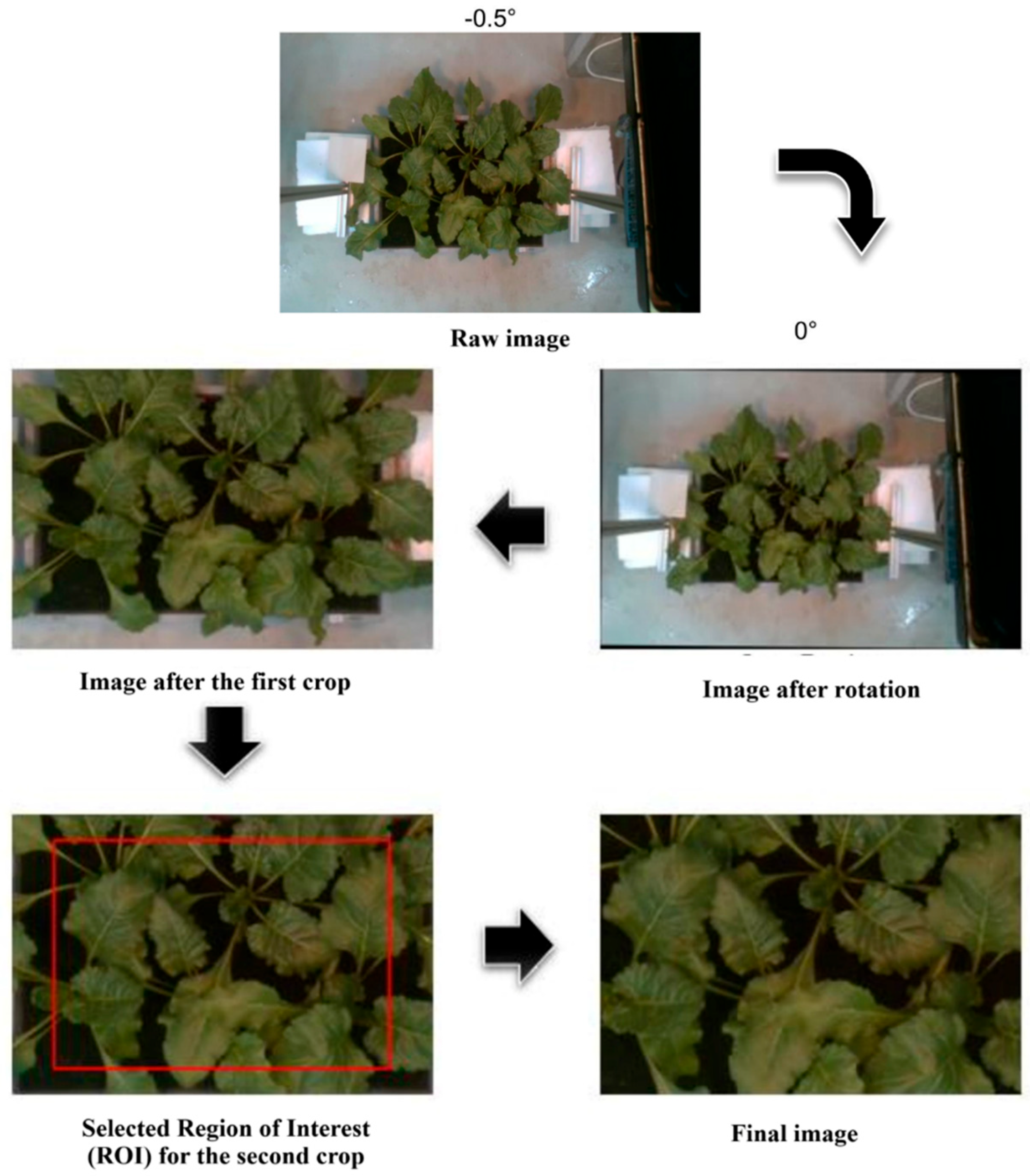
Figure 2.
Workflow of the proposed machine learning-based stress detection system. a) Phase 1. Preprocessing of raw RGB images and feature extraction to generate input data sets. (b) Phase 2. Four machine modules designed to identify and classify four respective stress conditions. c) Water Stress Existence Machine Module using RGB input to SVM algorithm, causing ‘sufficient’ water classification.
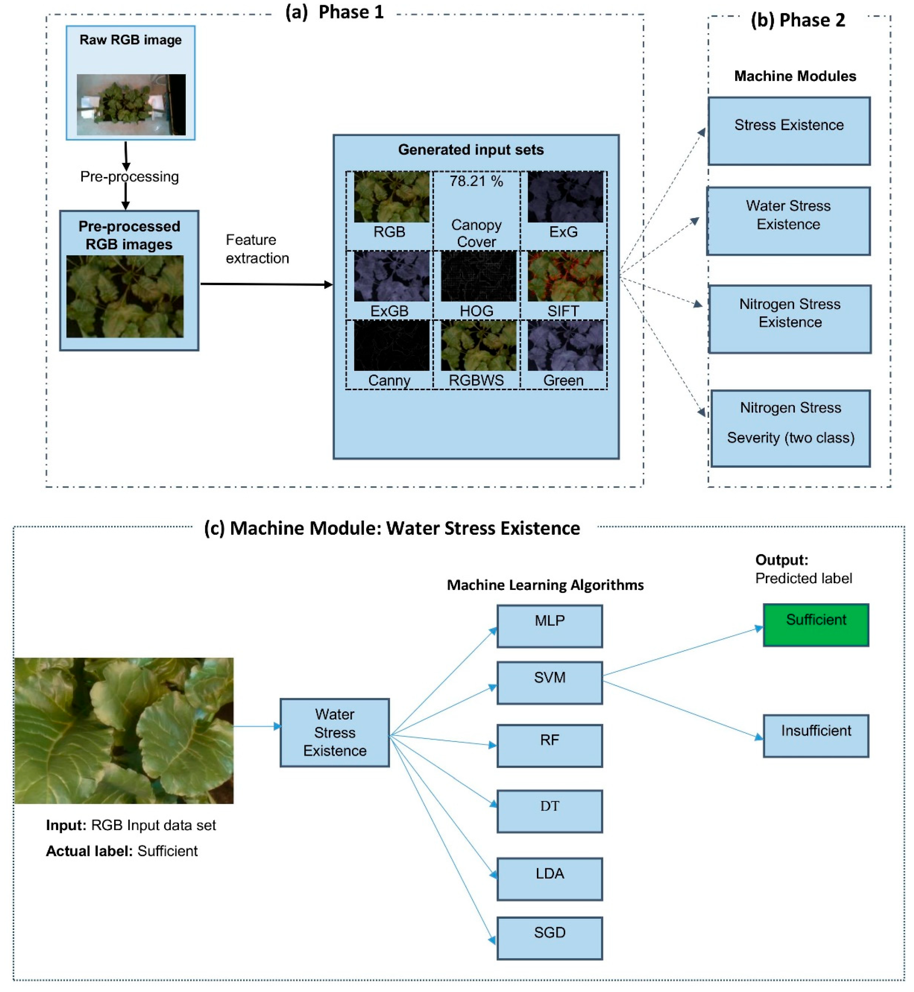
Figure 3.
A hidden layer MLP example for classifying into two classes.
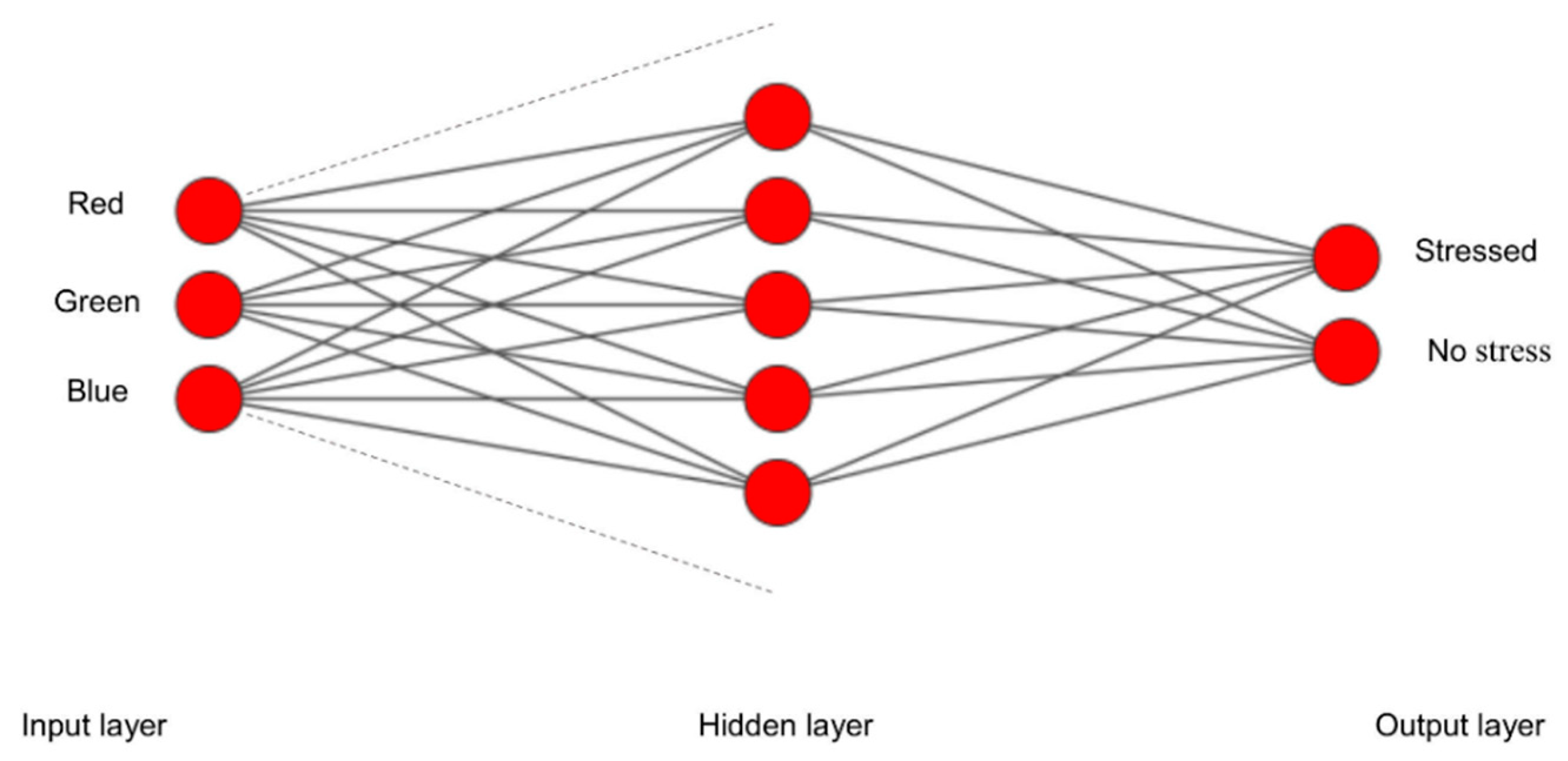
Figure 4.
MLIMs' accuracy in detecting stress for testing data set.
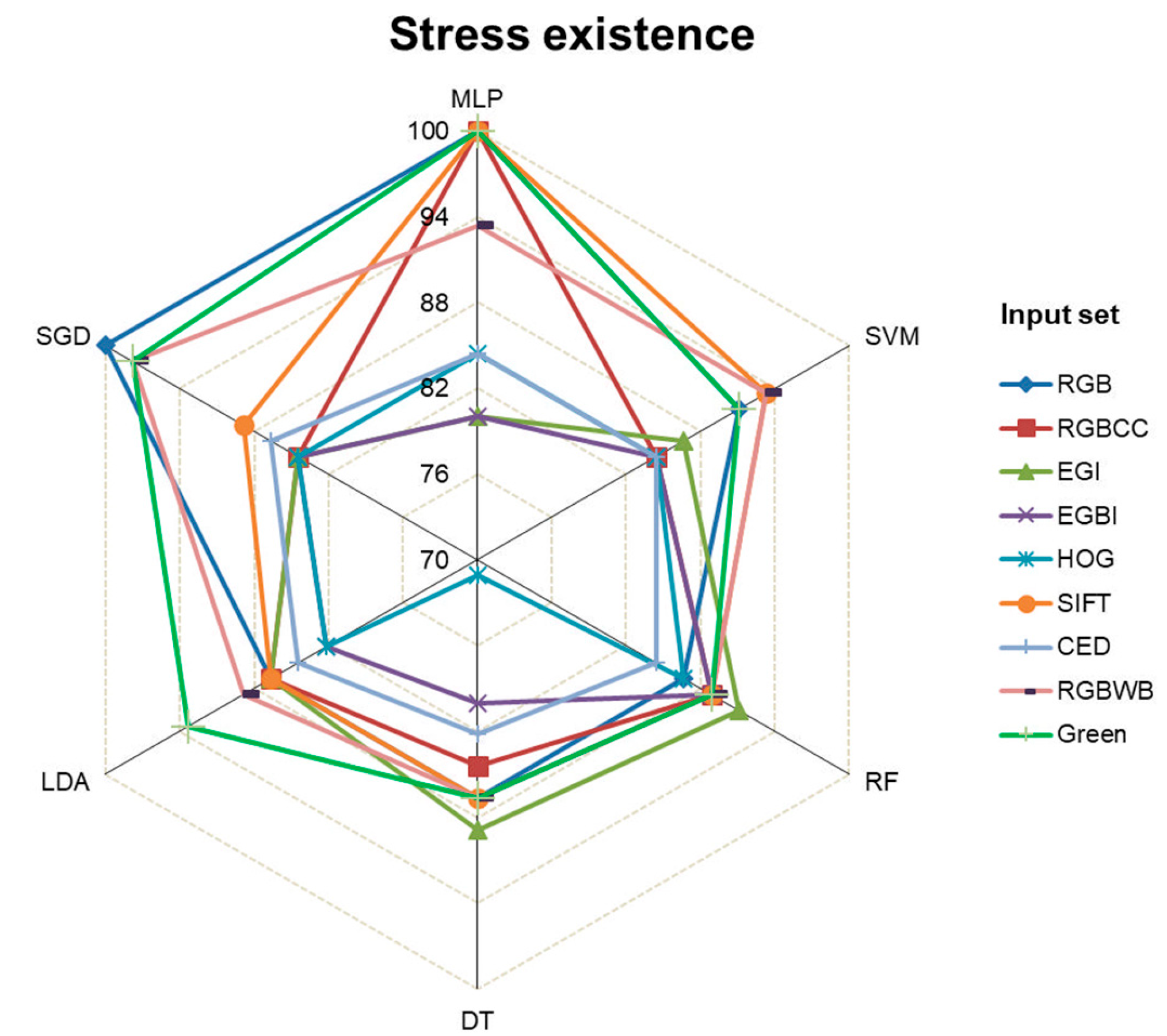
Figure 5.
The confusion matrix of the most accurate MLISs for detecting stress existence during testing.
Figure 5.
The confusion matrix of the most accurate MLISs for detecting stress existence during testing.
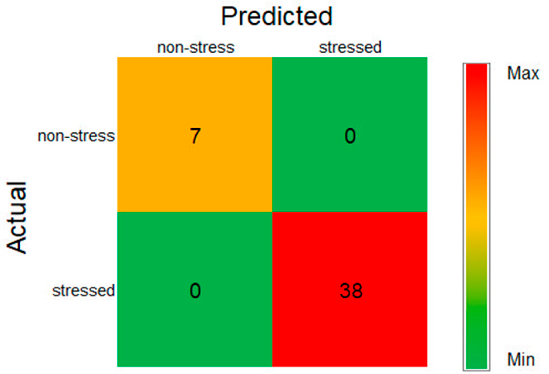
Figure 6.
Test Accuracy of different MLIMs for detecting water stress (a), nitrogen stress at three levels (b), and nitrogen stress at two levels (c).
Figure 6.
Test Accuracy of different MLIMs for detecting water stress (a), nitrogen stress at three levels (b), and nitrogen stress at two levels (c).
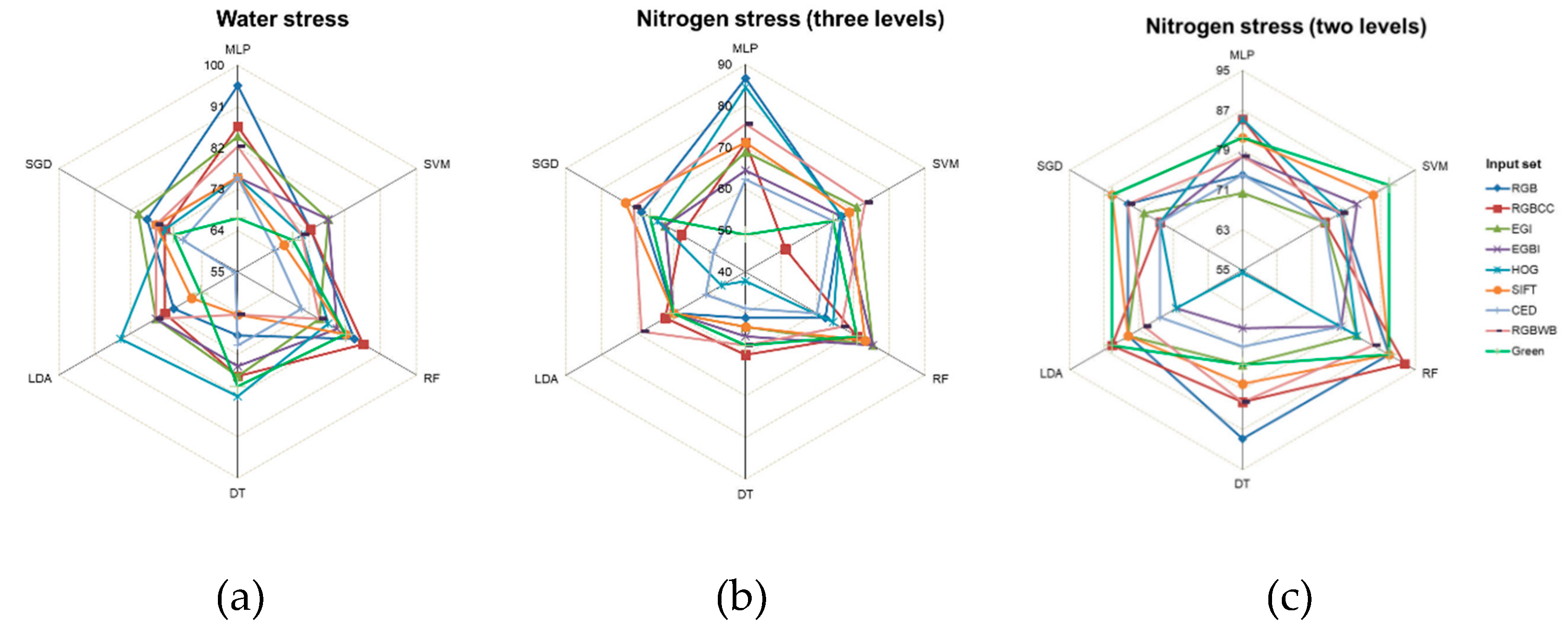
Figure 7.
The confusion matrix of the most accurate MLISs during Testing, for detecting: (a) Water stress (45 images); (b) Nitrogen stress at three levels (27 images), and (c) Nitrogen stress at two levels (45images).
Figure 7.
The confusion matrix of the most accurate MLISs during Testing, for detecting: (a) Water stress (45 images); (b) Nitrogen stress at three levels (27 images), and (c) Nitrogen stress at two levels (45images).
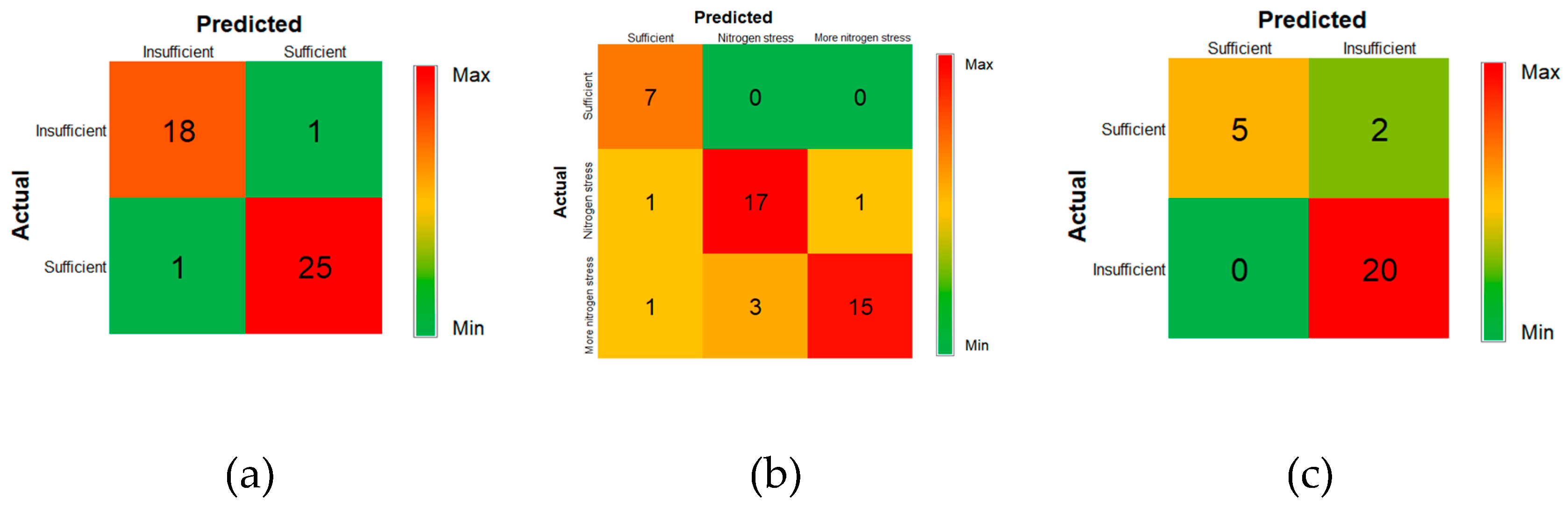
Figure 8.
Testing Execution time(s) for different MLISs.
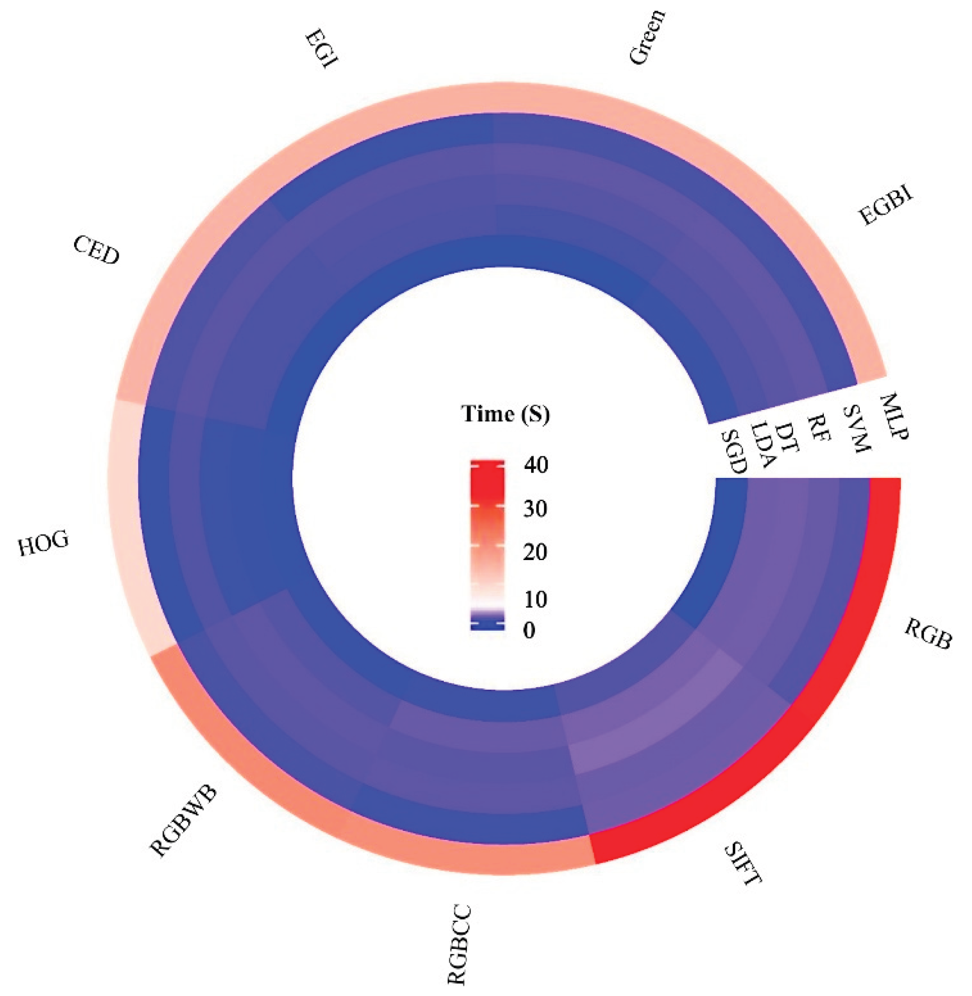
Table 1.
The description of the treatment used in this study.
| Treatment | Replication | Water input | Nitrogen input |
| Control | 3 | Sufficient | Sufficient |
| More Nitrogen Stress | 3 | Sufficient | Low |
| Nitrogen stress | 3 | Sufficient | Medium |
| Water stress | 3 | Insufficient | Sufficient |
| Water stress – Nitrogen stress | 3 | Insufficient | Low |
Table 2.
Input datasets used in this study.
| Row | Input sets | Abbreviation | Number of input sets | Reference |
| 1 | Red – Green – Blue bands (RGB image) | RGB | 3 | ____ |
| 2 | RGB image and Fractional Canopy Cover | RGBCC | 4 | This study |
| 3 | Excess Green index | EGI | 1 | [38] |
| 4 | Excess Green minus excess Blue Index | EGBI | 1 | [39] |
| 5 | Histogram of Oriented Gradients descriptor | HOG | 1 | [40] |
| 6 | Scale-Invariant Feature Transform descriptor | SIFT | 3 | [41] |
| 7 | Canny Edge Detector | CED | 1 | [42] |
| 8 | RGB image without background pixels | RGBWB | 3 | This study |
| 9 | Green band | Green | 1 | ____ |
Table 3.
Statistical result of the most accurate MLIMs for detecting stress existence.
| Method | Statistical Parameter | ||||||
| MLP and SGD with RGB | Accuracy (%) | Loss | Precision (%) | Recall (%) | F1-score (%) | ||
| Training | Test | Training | Test | ||||
| 100 | 100 | 0.0017 | 0.0525 | 100 | 100 | 100 | |
Table 4.
Statistical result of the best MLIM for detecting water stress, nitrogen stress at three levels, and nitrogen stress at two levels.
Table 4.
Statistical result of the best MLIM for detecting water stress, nitrogen stress at three levels, and nitrogen stress at two levels.
| Stress type | Method | Statistical Parameter | ||||||
| Accuracy (%) | Loss | Precision (%) | Recall (%) | F1-score (%) | ||||
| Training | Test | Training | Test | |||||
| Water stress | MLP and RGB | 100 | 95.56 | 0.01 | 0.28 | 95.56 | 95.56 | 95.56 |
| Nitrogen-V1a | MLP and RGB | 100 | 86.67 | 0.02 | 0.65 | 87.57 | 86.67 | 86.61 |
| Nitrogen-V2b | RF and RGBCC | 100 | 92.59 | 0.18 | 0.49 | 93.27 | 92.59 | 92.15 |
a: Nitrogen stress at three levels (severity of nitrogen stress). b: Nitrogen stress at two levels (existence of nitrogen stress).
Table 5.
Determining the most appropriate input sets when considering both time and accuracy simultaneously.
Table 5.
Determining the most appropriate input sets when considering both time and accuracy simultaneously.
| Weight | MLA | ||||||
| Accuracy | Time | MLP | SVM | RF | DT | LDA | SGD |
| 1 | 1 | SIFT | EGBI | EGBI | EGI | RGB | Green |
| 0.3 | 0.7 | SIFT | RGB | EGBI | EGI | RGB | Green |
| 0.7 | 0.3 | SIFT | Green | Green | RGB | Green | SIFT |
Table 6.
Determining the most appropriate machines considering both time and accuracy simultaneously.
Table 6.
Determining the most appropriate machines considering both time and accuracy simultaneously.
| Weight | Input set | |||||||||
| Accuracy | Time | RGB | RGBCC | EGI | EGBI | HOG | SIFT | CED | RGBWB | Green |
| 1 | 1 | SGD | RF | SVM | SVM | RF | MLP | RF | SGD | SGD |
| 0.3 | 0.7 | SGD | RF | SVM | SVM | RF | MLP | RF | SGD | SGD |
| 0.7 | 0.3 | SGD | RF | SVM | SVM | RF | MLP | RF | SGD | SGD |
Disclaimer/Publisher’s Note: The statements, opinions and data contained in all publications are solely those of the individual author(s) and contributor(s) and not of MDPI and/or the editor(s). MDPI and/or the editor(s) disclaim responsibility for any injury to people or property resulting from any ideas, methods, instructions or products referred to in the content. |
© 2025 by the authors. Licensee MDPI, Basel, Switzerland. This article is an open access article distributed under the terms and conditions of the Creative Commons Attribution (CC BY) license (http://creativecommons.org/licenses/by/4.0/).
Copyright: This open access article is published under a Creative Commons CC BY 4.0 license, which permit the free download, distribution, and reuse, provided that the author and preprint are cited in any reuse.


