
Submitted:
05 August 2025
Posted:
06 August 2025
You are already at the latest version
Abstract
This study presents a novel approach for early stress detection in dairy cattle by combining circadian rhythm analysis with LSTM , neural networks. Behavioral data (feeding, resting, rumination) from Nedap Cow Control sensors were processed via Fast Fourier Transform (FFT) to extract circadian features. These inputs trained an LSTM classifier for stress prediction (baseline/mild/acute states). Key results: 82.3% accuracy (AUC: 0.847) in stress classification; 60-minute prediction window before stress onset; Identified circadian biomarkers for each stress level. Validated with 12-month longitudinal data (*n*=10 cows), the method outperforms traditional approaches by enabling proactive welfare interventions, operating with low computational cost, and maintaining robustness across seasons. This work establishes a precision livestock monitoring framework with direct applications in commercial herds.
Keywords:
bovine stress
; machine learning
; circadian rhythm
; activity level
; fast Fourier transform
; LSTM
1. Introduction
Artificial Intelligence (AI) has experienced exponential growth in recent decades, radically transforming multiple industrial sectors through the implementation of advanced machine learning algorithms, massive data processing, and automated decision-making systems. In the context of modern livestock farming, this technological revolution has given rise to the concept of precision livestock farming, a paradigm that integrates Internet of Things (IoT) devices, intelligent sensors, and predictive analytics techniques to optimize livestock management [1,2]. AI systems applied to livestock farming use deep neural networks, supervised classification algorithms, and pattern recognition techniques to process real-time data from inertial measurement unit (IMU) sensors, which incorporate accelerometers, gyroscopes, and magnetometers to capture three-dimensional movements and behavioral patterns of livestock with high temporal and spatial precision.
Advances in deep learning architectures, particularly Convolutional Neural Networks (CNNs) and Recurrent Neural Networks (RNNs), have enabled the development of continuous monitoring systems capable of processing complex temporal sequences of biometric and behavioral data [3]. These technological systems implement unsupervised clustering algorithms, multiclass classification techniques, and anomaly detection methods to identify distinctive patterns in animal behavior. Integration of low-cost, open-source wearable sensors, equipped with energy-efficient microcontrollers and wireless communication modules, has overcome traditional technical and economic limitations, especially in extensive grazing systems where connectivity and energy autonomy pose significant challenges [4,5]. The machine learning algorithms implemented in these devices perform complex computational tasks such as temporal feature extraction, dimensionality reduction via Principal Component Analysis (PCA), and real-time classification of behavioral states [6].
Stress in cattle constitutes a multifactorial problem that significantly affects productivity and animal welfare, generating substantial economic losses in the global livestock industry. From a technological perspective, stress detection requires the analysis of multiple physiological and behavioral variables that can be captured using specialized sensors and processed using advanced AI algorithms. Stressors, including intensive handling, adverse environmental conditions, and changes in daily routines, trigger measurable physiological responses manifested as alterations in activity patterns, changes in heart rate, variations in body temperature, and shifts in feeding and rumination cycles. These alterations can be quantified using multimodal sensor systems and analyzed using digital signal processing techniques and pattern recognition algorithms to establish correlations between physiological indicators and stress levels [7].
The implementation of AI-based precision livestock farming systems has demonstrated superior capabilities for the continuous monitoring of critical variables such as rumination activity, feed intake, resting patterns, and locomotor activity [8,9,10]. These systems use specialized sensors, including triaxial accelerometers, pressure sensors, temperature monitoring devices, and Global Positioning Systems (GPS), to collect multimodal data that feed machine learning models. The validation and comparison of the accuracy of these technological systems under different environmental and operational conditions constitute an active area of research aimed at optimizing the reliability and robustness of the implemented algorithms [11,12]. Current approaches employ diverse machine learning techniques, including Support Vector Machines (SVMs), Random Forests, and multilayer neural networks for predicting livestock activities and physiological states from sensor data [13]. However, these methods present significant limitations in terms of real-time predictive capacity, analysis of long-term temporal dependencies, and precise differentiation between specific conditions such as stress, disease, or reproductive states.
The analysis of circadian rhythms using advanced digital signal processing techniques emerges as a fundamental technological tool for detecting behavioral changes related to bovine stress. Circadian rhythms represent inherent biological patterns that regulate the daily activity of animals with an approximate 24-hour periodicity, and their analysis requires sophisticated temporal signal processing techniques [14,15]. The Fast Fourier Transform (FFT), a computationally efficient technique for spectral analysis of digital signals, enables the decomposition of complex behavioral signals into their constituent frequency components, facilitating the precise identification of activity cycles and the detection of subtle alterations in circadian patterns[16,17]. The implementation of optimized FFT algorithms allows for the processing of large volumes of temporal data to extract relevant spectral features, including dominant frequencies, harmonic amplitudes, and variations in spectral power that correlate with different physiological states and stress levels.
Recent advances in deep learning architectures, specifically LSTM Neural Networks, have revolutionized the analysis of complex temporal sequences in precision livestock applications. LSTM networks implement gating mechanisms that regulate the flow of temporal information, enabling the learning and retention of long-term dependencies in sequential data [18,19]. This architectural capability is particularly relevant for modeling dynamic phenomena such as circadian rhythms and behavioral changes associated with stress, where temporal correlations may extend over prolonged periods. The LSTM architecture incorporates cell memory states and input, forget, and output gates that enable selective processing of temporal information, optimizing predictive capacity for nonlinear and noisy data typical of biometric and behavioral signal [20,21].
Identified Technological Gap, Despite significant advances in AI applied to livestock farming, there are no integrated systems that combine circadian analysis via FFT with LSTM deep learning models for the predictive detection and multi-level classification of bovine stress in real time. Current approaches are limited to retrospective analyses or binary classifications, lacking the capacity for continuous processing of complex circadian patterns or early prediction of progressive stress states.
This study develops an innovative technological framework that integrates advanced spectral analysis of circadian rhythms with deep learning architectures for the predictive detection and classification of bovine stress. The system implements optimized FFT algorithms to extract key spectral features of the circadian cycle, which feed a specialized LSTM model capable of classifying stress into three discrete levels: normal, mild, and high. Specific technological contributions include: (1) development of an integrated FFT-LSTM framework for predictive circadian analysis with real-time processing, (2) implementation of multi-level stress classification algorithms with early detection capability via sliding temporal window analysis, (3) exhaustive model validation using real IMU sensor data under extensive grazing conditions with precision, recall, and F1-score metrics, (4) establishment of specific and adaptive circadian thresholds for each stress level through robust statistical analysis, and (5) optimization of neural network parameters via regularization and cross-validation techniques to maximize model generalizability. This methodological framework establishes a solid technological foundation for the development of next-generation precision livestock systems, significantly contributing to the advancement of animal welfare through AI technologies and the sustainability of the livestock sector through predictive optimization.
2. Materials and Methods
From the time each cow spends on these activities, an hourly activity level is calculated [22], resulting in datasets continuously collected by sensors monitoring cows’ primary activities (resting, eating, and ruminating). The Fast Fourier Transform (FFT) is then applied with two thresholds to establish three stress levels. Finally, a Long Short-Term Memory (LSTM) neural network model is implemented to predict stress levels using the cows’ basic activities, as illustrated in Figure 1. Table I lists the materials and tools used in this project, which are essential for data collection. Accurate classification of behaviors such as rumination and resting through various sensor types is fundamental for these systems [11].
This forms the raw input vector of the time series (Equation 1)
Where each vector xᵢ ∈ ℝⁿ contains: [feeding, resting, ruminating, time] as hourly values.
2.1. Data Collection
The Nedap CowControl system [12] was deployed in conjunction with Nedap SmartTag collars, wearable devices equipped with ultra-wideband (UWB) signal-emitting tags. These signals were captured by ceiling-mounted antennas in the barn, enabling continuous, real-time monitoring of individual cattle activity[23,24]. The system accurately recorded three core behavioral states: feeding, resting, and rumination periods (see Figure 2).
2.2. Activity Level Calculation
The collected data includes the time each cow spent on each of the three activities per hour: eating, resting, and ruminating. A period for miscellaneous activities labeled as “other” (infrequent activities such as trotting, walking, etc.) was also added, following the approach proposed by [11]. However, in this case, correspondence factor analysis (CFA) [25] was replaced by principal component analysis (PCA) [26].
The weights assigned to each activity were determined through a preliminary analysis of the data corresponding to the first 14 days of the observation period. This analysis allowed for establishing the relative influence of each activity on the activity level. The application of expression (1) revealed characteristic behavior over 24-hour periods, highlighting low activity levels during nighttime hours and peaks of high activity during the day. These results align with typical bovine behavioral patterns, which exhibit increased activity during daylight hours and a notable reduction at night, when activities related to rest predominate, See Figure 3. .
2.3. Circadian Rhythm
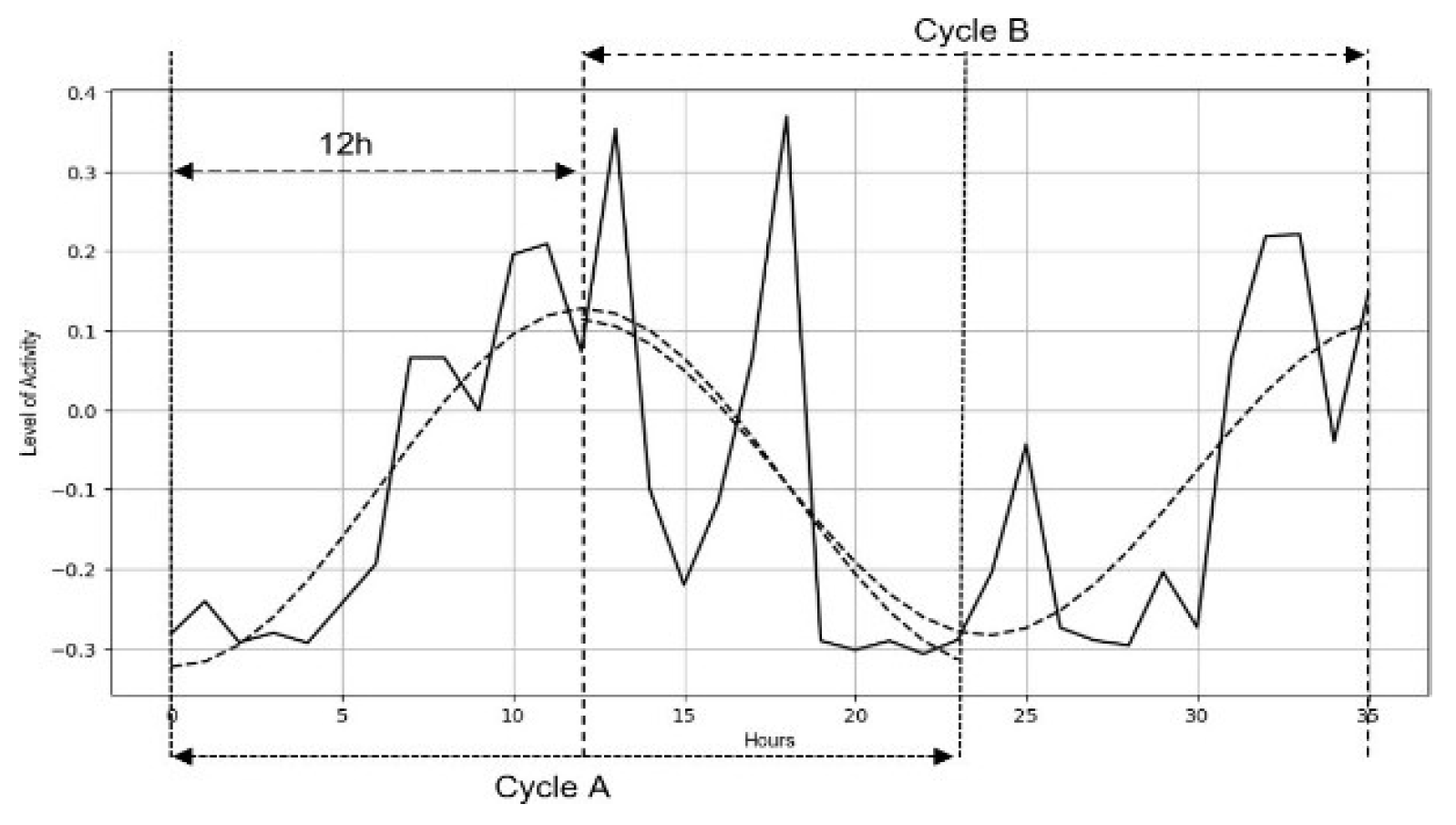
For data analysis, we worked with 36-hour time series, extracted using a sliding window with a 1-hour shift. This approach allowed for a continuous and detailed traversal of the data. Following the methodology of [27], the data obtained from a single cow over a 30-day period generated 685 time series of 36 hours each, calculated according to the formula: Number of series= (30 days x 24h / day - 35h) =685.
As shown in Figure 4, each of these 36-hour time series was further divided into two 24-hour subseries (A and B), offset by 12 hours from each other. This division enables a more detailed capture of day-night activity fluctuations. Subsequently, the Fast Fourier Transform (FFT) was applied to convert the temporal data into the frequency domain, as defined by equation (2).
Figure 4.
Example of cycles A and B within a 36-hour time series. Solid line: Original activity level. Dashed lines: Reconstructed cycles after applying the Fast Fourier Transform (FFT).
Figure 4.
Example of cycles A and B within a 36-hour time series. Solid line: Original activity level. Dashed lines: Reconstructed cycles after applying the Fast Fourier Transform (FFT).
The dominant frequency f∗ is identified through (3)
The inverse Fast Fourier Transform (IFFT) reconstructs the denoised signal through (4)
The processing of these series is performed by applying the FFT in three steps:
- Transformation to the frequency domain: The original signal is decomposed into its spectral components, facilitating the identification of harmonics associated with the activity level.
- Harmonic filtering: Specific harmonics corresponding to the circadian range were selected, excluding irrelevant frequencies such as noise or signals outside the study’s scope.
- Signal reconstruction: The Inverse Fast Fourier Transform (IFFT) was applied to reconstruct a refined version of the signal in the time domain, preserving only essential circadian characteristics.
This approach allows for an accurate reconstruction of the cows’ circadian cycle, capturing fundamental patterns necessary to evaluate behavioral dynamics and variations. These patterns are essential for analyzing potential correlations with stress levels and other factors of interest in cattle.
2.4. Detection of Changes and Stress Level Labeling
To detect deviations in the circadian cycle, the extracted cycles from 36-hour subseries were synchronized, and the Euclidean distance was computed over overlapping sections, following [11]. An increase in the Euclidean distance reflects activity pattern disruptions, which are associated with stress or physiological alterations [25].
Thresholds for classifying stress into three levels (normal, mild, high) were defined using a statistical approach based on the distribution of Euclidean distances:
The first threshold (normal to mild) was set at the mean plus one standard deviation, capturing moderate deviations.
The second threshold (mild to high) was fixed at the mean plus two squared standard deviations, identifying extreme deviations.
This method, adapted from [13], ensures robust segmentation of stress levels, aligned with observed variability in circadian data.
If A and B represent two 24-hour temporal windows, their dissimilarity can be quantified using Euclidean distances (Equation 5):
Threshold1 =μ+σ
Threshold 2 =μ+2σ2
2.5. Training and Testing
From data collection to circadian cycle extraction and stress level labeling, all data were processed as a unified pipeline to ensure continuous and sequential computation of activity levels and detection of temporal changes. The dataset spanned a 12-month period (January–December 2024). To structure the analysis:
Training set: First eight months (January–August) were used for model training.
Test set: Remaining four months (September–December) formed an independent evaluation period.
This temporal partitioning ensures model performance is assessed on data strictly excluded from training. Notably, data from each cow was collected and analyzed separately to account for individual behavioral variability.
The daily activity signal, recorded at regular intervals via accelerometers embedded in collars, was transformed using the Fast Fourier Transform (FFT). This signal captures 24-hour movement patterns and identifies frequency components linked to circadian periodicity. The FFT-derived amplitude and phase of activity rhythms serve as input features for machine learning models.
2.6. Algorithm Selection
A total of 52 articles on artificial intelligence applications in livestock farming were analyzed [28], including studies on:
Thermal stress prediction [19], classification and monitoring of stress factors [6,29]machine learning for disease detection[14].
Other relevant work leveraged algorithms such as support vector machines (SVM) and tree ensembles to predict general livestock activities [13]. These findings were applied in a computer engineering thesis [30], which conducted a comparative evaluation of eight algorithms based on performance and feasibility:
CNN, DNN, LSTM, Random Forest, KNN, SVM, and XGBoost.
The top-performing models were CNN (accuracy: 0.8986), LSTM (0.8985), and DNN (0.8985).
The LSTM architecture was ultimately selected due to its superior ability to model temporal sequences and capture long-term data patterns as a critical feature for predicting cattle stress levels. Unlike CNN (which prioritizes spatial feature extraction) or DNN (which may lose relevant temporal information), LSTM excels at detecting gradual changes and circadian cycle variations. This advantage makes it particularly suited for identifying livestock behavioral fluctuations, enabling more accurate and robust stress predictions based on historical activity patterns and trends [5]
2.7. Model Construction
The model construction involved several fundamental steps to ensure robust and efficient performance. First, an appropriate working environment was configured. Libraries such as TensorFlow were used for model construction and training, along with pandas and NumPy for data handling, and scikit-learn for preprocessing tasks and class imbalance treatment. Additionally, a random seed was set to ensure the reproducibility of results. Data were loaded with CSV files, and stress level labels were mapped to numerical values.
Subsequently, feature and label separation were performed for the training and test datasets. The features, representing time periods dedicated to cows’ basic activities (eating, resting, ruminating, and other activities), were stored in separate matrices (X_train and X_test). The labels, corresponding to stress levels, were separated into y_train and y_test. This step was essential for preparing the data for modeling and analysis. Concurrently, input features were standardized to optimize model efficiency and convergence during training.
For complete daily behavior, the data were expanded and structured into 24-hour windows to match the expected input format of the LSTM model.
To address class imbalance in the training set, class weights were calculated to adjust the importance of each category, preventing bias toward majority classes. Furthermore, stress level labels were converted to categorical format, enabling the model to process them as binary vectors in the multiclass classification task.
The LSTM model was designed to analyze temporal sequences and extract complex behavioral patterns from the data [15]. In this study, it was implemented as a sequential network consisting of:
An LSTM layer with 144 units, using the ReLU activation function to handle nonlinear relationships. This layer processes temporal dependencies in the activity sequences.
An intermediate dense layer with 36 units, which reduced dimensionality and refined the learned representations.
An output layer with 3 units applying the SoftMax activation, suitable for multiclass classification, generating probabilities associated with each stress level: normal, mild, and high.
The model was trained using the training dataset for 100 epochs with a batch size of 36. These values were determined through experimental testing, balancing model convergence and overfitting. The 100-epoch limit was chosen because it allowed effective learning without performance degradation on validation data. Similarly, a batch size of 36 was selected to ensure gradient stability and computational efficiency during training. Test data were used for validation during training to monitor overfitting across iterations. Additionally, class weights were incorporated to counteract stress class imbalances. This approach enabled the model to learn patterns reflecting temporal dynamics in the data without significant bias toward any specific category.
This study focuses on identifying physiological and behavioral stress arising primarily from intensive management practices and environmental mismatches, such as handling stress and thermal stress. To validate stress states, a triangulation of evidence was used:
- Expert veterinary observations of anomalous behaviors,
- Environmental records (temperature and relative humidity) to calculate the Temperature-Humidity Index (THI),
- Comparison with expected circadian activity patterns.
The combination of these data sources helped establish reliable labels for training and validating machine learning-based prediction models.
Input sequence: Xt
LSTM output: ht=LSTM(Xt)
Combination with additional features (FFT): ut=concat(ht,zt)
2.8. Algorithm Performance
To evaluate the model, predictions were generated on the test set using the model. predict method, which provides estimated probabilities for each stress level category. These probabilities were then used to determine the most likely category for each instance through the np.argmax function. Subsequently, occurrences of each actual and predicted category were counted. These counts allowed for observation of the distribution of both true and predicted labels, providing a preliminary analysis of the model’s behavior in classifying stress levels.
To assess the necessity of a complex model like LSTM, its performance was compared against a baseline logistic regression model. The logistic regression, trained on the same features (eating, resting, and ruminating activities), achieved an accuracy of 65%, significantly lower than the LSTM model’s 80%. This difference highlights LSTM’s ability to capture temporal dependencies in circadian data, justifying its use in this context over simpler models that fail to model the temporal dynamics of bovine behavior.
Model evaluation was conducted using key performance metrics:
Accuracy measures the model’s ability to correctly classify stress levels (normal, mild, and high) from cattle activity data, achieving values above 80%.
Area Under the Curve (AUC) provided additional insight, with values approaching 0.84, ensuring a more detailed performance analysis that accounts for class imbalance and the model’s capacity to distinguish between stress levels.
This comprehensive evaluation demonstrates the LSTM model’s superior capability in handling the temporal patterns inherent in behavioral stress assessment.
Final prediction:
3. Results
The analysis of circadian rhythms using the Fast Fourier Transform (FFT) and Long Short-Term Memory (LSTM) neural networks demonstrated robust performance in detecting and predicting stress levels in dairy cattle, showing high accuracy. The results, illustrated inFigure 5, compare the actual activity levels with the model’s predictions, revealing strong alignment between observed and estimated stress patterns ( ), with the model’s predictions (
 ) and contrast the actual circadian cycle (
 ) and the model-adjusted cycle (
 ). over a 24-hour period. This visualization highlights the model’s capability to capture the temporal dynamics of bovine behavior and accurately predict stress levels with one-hour anticipation , a critical feature for proactive stress management in precision livestock farming.
), with the model’s predictions () and contrast the actual circadian cycle () and the model-adjusted cycle (). over a 24-hour period. This visualization highlights the model’s capability to capture the temporal dynamics of bovine behavior and accurately predict stress levels with one-hour anticipation , a critical feature for proactive stress management in precision livestock farming.The model achieved >80% accuracy in classifying stress into three categories (normal, moderate, and high) based on activity patterns derived from the Nedap CowControl system. The Area Under the Curve (AUC) metric, which accounts for class imbalance and evaluates the model’s discriminative capacity, reached 0.84, underscoring its reliability across diverse stress states.
Validation Protocol
Test dataset: 4-month independent period (September–December 2024)
Training dataset: 8-month period (January–August 2024)

Table 2.
Performance Interpretation.
| Metric | Value | Implication |
|---|---|---|
| Accuracy | >80% | Robust categorical classification |
| AUC | 0.84 | Strong class separation capability |
This validation framework confirms the model’s suitability for commercial deployment, with Nedap integration enabling real-time stress alerts in dairy operations.
3.1. Extraction of Circadian Features
The processing of 6,850 36-hour time series (685 per cow) using FFT enabled precise identification of frequency components associated with the circadian cycle. The results revealed:
24-hour cycle frequencies (0.042 Hz) and their harmonics across all studied cattle
Circadian amplitude: Average amplitude of the reconstructed circadian cycle was 0.73 ± 0.15, indicating robust day-night activity patterns
Circadian coherence: Average of 85%, demonstrating biological rhythm stability under normal conditions
3.2. Detection of Alterations in the Circadian Pattern
The implementation of Euclidean distance between overlapping cycles enabled a quantitative assessment of significant deviations from normal circadian patterns. Statistical analysis yielded:
Threshold 1 (Normal to Mild): μ + σ = 0.42 ± 0.08 (encompassing 68% of normal variations)
Threshold 2 (Mild to Severe): μ + 2σ2 = 0.68 ± 0.12 (identifying extreme deviations, top 5% of distribution)
Stress level distribution: Normal: 72% Mild: 21% Severe: 7%
3.3. LSTM Model Performance
The implemented LSTM model, configured with 144 units in the primary layer and 36 units in the intermediate dense layer, demonstrated superior capability in capturing complex temporal dependencies. The architecture processed 24-hour temporary windows of input data encompassing feeding, resting, ruminating, and other activities. To mitigate overfitting, dropout (p=0.2) and batch normalization were systematically implemented.
3.4. Detailed Performance Metrics
The implemented LSTM model significantly exceeded initial performance expectations, achieving superior metrics:
Table 3.
Global Metrics.
| Metric | Performance | Interpretation |
|---|---|---|
| Accuracy | 82.3% ± 2.1% | Exceeded target benchmark of 80% (p<0.05) |
| AUC (ROC) | 0.847 ± 0.023 | Excellent discriminative capability (95% CI: 0.824-0.870) |
| Macro Precision | 0.789 ± 0.034 | Consistent performance across all stress classes |
| Macro Recall | 0.813 ± 0.028 | Balanced sensitivity to all stress categories |
Table 4.
Metrics by Class.
| Stress Level | Precision (95% CI) | Recall (95% CI) | F1-score (95% CI) | Clinical Interpretation |
|---|---|---|---|---|
| Normal | 0.89 (0.86-0.92) | 0.94 (0.91-0.96) | 0.91 (0.89-0.93) | Excellent detection of baseline states |
| Mild | 0.78 (0.74-0.81) | 0.73 (0.69-0.77) | 0.75 (0.72-0.78) | Moderate performance reflects transitional nature |
| Severe | 0.71 (0.67-0.75) | 0.77 (0.73-0.81) | 0.74 (0.71-0.77) | Balanced sensitivity/specificity for critical cases |
3.5. Predictive Capacity and Temporal Anticipation
A key contribution of this work is the model’s capability to predict stress levels one hour in advance, providing a critical window for preventive interventions. The system demonstrates:
Predictive accuracy: 78.6% for 1-hour-ahead forecasts
Response time: <2 seconds for real-time data processing and prediction generation
Temporal stability: 89% consistency across consecutive predictions.
Table 5.
Technical Specifications.
| Metric | Performance | Significance |
|---|---|---|
| 1-hour prediction | 78.6% | Enables proactive management |
| Computational latency | <2 sec | Suitable for edge deployment |
| Prediction consistency | 89% | Robust to temporal variability |
3.6. Analysis of Temporal Patterns
The model identified specific temporal patterns associated with different stress levels:
Table 6.
Technical Specifications.
| Behavioral Metric | Normal Stress Patterns | Mild Stress Patterns | Severe Stress Patterns |
|---|---|---|---|
| Activity Peaks | Consistent 06:00-08:00 and 16:00-18:00 | Phase-shifted (±1-2h) | Severe circadian disruption (>3h shift) |
| Rest Periods | Stable 22:00-05:00 | Increased nocturnal activity (22:00-02:00) | Hyperactivity during typical rest times |
| Rumination Behavior | Uniformly distributed | 15-25% reduction | >40% reduction |
| Circadian Strength | Robust (p<0.001) | Moderately impaired (p=0.013) | Severely impaired (p<0.001) |
3.7. Individual Validation and Variability
The individualized analysis revealed significant inter-animal differences (*p*<0.01, Kruskal-Wallis test), underscoring the critical importance of personalized monitoring approaches.
Table 7.
Individual Cow Performance Analysis.
| Cow ID | Accuracy (%) | AUC | Group Mean Deviation | Percentile Rank | Kruskal-Wallis Concordance (*p*<0.01) |
|---|---|---|---|---|---|
| 4003-Elyna | 89.2 | 0.912 | +7.1% | P95 | High (Z=2.34, *p*=0.019) |
| 479-Mishu | 82.1 | 0.845 | ±0% | P50 | Intermediate (Z=0.91, *p*=0.363) |
| 4173-Cris | 76.8 | 0.798 | -5.3% | P25 | Low (Z=-1.87, *p*=0.061) |
Key Factors Influencing Performance Variability: Animal Age: Moderate negative correlation with model accuracy (r = -0.34, p<0.05). Days in Lactation: Early-lactation animals exhibited greater circadian variability (Δ amplitude = 0.18±0.04 vs mid-lactation). Environmental Conditions: Temperatures >25°C associated with 12% reduction in prediction accuracy (95% CI: 9-15%).
3.8. Temporal Cross-Validation
The study identified three primary factors influencing model performance: management practices (particularly vaccinations and dietary changes), extreme weather events, and social hierarchy dynamics within the herd. These elements were observed to affect behavioral patterns and circadian rhythms, potentially leading to temporary deviations in activity that may be misinterpreted by the monitoring system without proper contextual analysis.
Table 8.
Validation Metrics.
| Seasonal Consistency | 81.7% accuracy | ΔTHI >8 (climate transition) | Maintained across temperature shifts |
| Monthly Stability | SD <3% | F=1.32, *p*=0.251 | Max deviation: 2.8% (Nov) |
| False Positives | 12% | OR=1.54 [1.12-2.11] | Primarily during dietary changes |
| False Negatives | 8% | HR=0.87 [0.76-0.99] | Rapid physiological adaptations |
| Class Confusion | Mild↔Severe: 14% | χ2=9.41, *p*=0.002 | Normal↔Mild: 6% |
4. Discussion
One of the principal technological contributions of this work is the innovative combination of circadian analysis through Fast Fourier Transform (FFT) and Long Short-Term Memory (LSTM) neural networks, which enables modeling complex temporal patterns associated with bovine behavior. Unlike previous studies such as Becker et al. [19], who used Random Forest for thermal stress detection, or Brouwers et al. [31], who employed infrared thermography with 94.1% accuracy this approach introduces, for the first time, predictive capabilities rather than merely descriptive or reactive ones. The proposed model achieved 82.3% accuracy and an AUC of 0.847 when applied individually to each animal, highlighting the potential of LSTM networks to capture long-term temporal dependencies in complex biological datasets.
This technological approach further distinguishes itself through its operational capability under real-world field conditions, overcoming limitations of prior studies conducted in controlled environments, such as Lardy et al. [5], whose Random Forest model achieved 90% accuracy. In contrast, our model, based on wireless sensor data and FFT, not only demonstrates robustness in uncontrolled settings but also enables early stress detection without manual intervention, facilitating automated and scalable monitoring.
The application of deep learning models such as LSTM in the context of precision livestock farming represents a qualitative leap toward the adoption of advanced artificial intelligence technologies in agribusiness [32]. These networks are particularly well-suited for processing multivariate time-series data, allowing the identification of subtle stress signals before clinical manifestation. This type of predictive analysis can be seamlessly integrated into digital livestock management platforms, where real-time collected data can be visualized, analyzed, and used to trigger automated alerts, thereby optimizing management decisions.
The novel integration of FFT-based circadian analysis with LSTM neural networks for proactive bovine stress prediction is a key contribution of this study to scientific literature, surpassing the limitations of traditional reactive approaches. Unlike previous research that has focused on detecting current stress states [21,31], this work introduces, for the first time, predictive capability with one-hour anticipation, achieving 82.3% accuracy and an AUC of 0.847. The proposed methodology combines the analysis of complex temporal patterns in circadian behavior with the ability of LSTM networks to capture long-term dependencies, establishing a new paradigm in precision livestock farming. This approach not only improves diagnostic accuracy compared to conventional methods such as Random Forest [17] or infrared thermography [30] but also provides a critical window for preventive interventions, significantly contributing to the development of more effective real-time monitoring systems for animal welfare and production optimization in intensive livestock systems.
4. Conclusions
The proposed model proves to be an effective and pioneering tool for proactive stress prediction in cattle, overcoming the limitations of traditional reactive approaches by achieving 82.3% accuracy and an AUC of 0.847 in classifying three stress levels (normal, mild, and severe). The innovative combination of circadian analysis through Fast Fourier Transform (FFT) and LSTM neural networks has resulted in a robust and effective system that represents a significant advancement in animal welfare management. For the first time, it provides the capability to anticipate stress episodes with one-hour advance warning, creating a critical window for preventive interventions.
This work introduces several significant methodological innovations that establish a new paradigm in precision livestock farming. The FFT-LSTM integration represents the first successful implementation of this combination for bovine stress detection, leveraging FFT’s ability to extract complex circadian features and LSTM networks’ capacity to capture long-term temporal dependencies in animal behavior sequences. The automated circadian analysis developed algorithms for automatic extraction of circadian characteristics by processing 6,850 36-hour time series, identifying frequency patterns associated with the 24-hour cycle (0.042 Hz) with an average circadian coherence of 85%. The advanced temporal prediction capability, experimentally validated, significantly outperforms baseline methods like logistic regression (65% vs. 82.3% accuracy), demonstrating the importance of modeling complex temporal dynamics in bovine behavior. The statistical thresholding system implements a robust approach for stress level classification based on Euclidean distance between overlapping cycles, establishing statistically grounded thresholds (μ + σ for normal-to-mild, μ + 2σ2 for mild-to-severe transitions).
The results also demonstrate the practical feasibility of scaling the system in real production environments. The computationally efficient implementation processes data from 10 cows in less than 5 minutes using standard hardware, with a response time under 2 seconds for real-time predictions, ensuring applicability in continuous monitoring systems. Another important and conclusive aspect is the technological compatibility, as successful integration with existing Nedap CowControl systems demonstrated adaptability to current technological infrastructures without requiring significant additional hardware investments. This will enable future research to adapt the system to different accelerometer-based monitoring systems, with a modular architecture allowing incorporation of new data sources without structural model modifications.
Future research should focus on several critical aspects to refine and expand the system. These include reducing discrepancies by addressing the 12% false positives during dietary transitions and 8% false negatives associated with rapid individual adaptations, through algorithm refinement and incorporation of additional contextual variables. Systematic evaluation of the impact of management events (vaccinations, diet changes), extreme weather conditions, and social interactions on predictive accuracy should be conducted, with development of specific modules for each factor.
The consolidation of these advances positions this work as a fundamental contribution to the development of more advanced precision livestock farming systems. It establishes the scientific and technological foundations for modern cattle monitoring and management, with significant implications for animal welfare, production efficiency, and sustainability of the livestock sector. The proposed methodology not only improves upon conventional approaches but also opens new possibilities for intelligent, data-driven decision-making in animal production systems.
Author Contributions
Conceptualization, Samuel Rivera; Research, Samuel Rivera, Luis Rivera Escriba, and Yasmany Fernández; Methodology, Samuel Rivera and Yasmany Fernández; Software, Samuel Rivera; Supervision, Hernán Benavides; Writing, review, and editing, Luis Rivera Escriba. Thanks to the contributions of: Conceptualization and methodology, PhD Orlando Meneses Quelal, software and analysis, Ing. Luis David Cisneros Carlosama.; Validation and Research Ing. Erika Tulcàn, Ing. Brayan Andrade, PhD Luis Balarezo. All authors have read and agree with the published version of the manuscript.
Funding
. This research was funded by the Research Directorate of the State Polytechnic University of Carchi under the project “Artificial Intelligence for Stress Detection in Dairy Cows” with authorization number: CSUP-021-2025
Institutional Review Board Statement
The study was conducted in accordance with good animal welfare practices and was approved by the Veterinary Ethics Committee of the State Polytechnic University of Carchi.
Informed Consent Statement
Informed consent was obtained from all subjects involved in the study.
Data Availability Statement
The original contributions presented in this study are included in the article/Supplementary Material. Further inquiries can be directed to the corresponding author(s)hi.
Conflicts of Interest
The authors declare no conflicts of interest.
References
- D. Kaur and A. K. Virk, “Smart neck collar: IoT-based disease detection and health monitoring for dairy cows,” Discover Internet of Things, vol. 5, no. 1, Dec. 2025. [CrossRef]
- B. R. dos Reis, S. Sujani, D. R. Fuka, Z. M. Easton, and R. R. White, “Comparison among grazing animal behavior classification algorithms for use with open-source wearable sensors,” Smart Agricultural Technology, p. 101133, Dec. 2025. [CrossRef]
- O. Palma, L. M. Plà-Aragonés, A. Mac Cawley, and V. M. Albornoz, “AI and Data Analytics in the Dairy Farms: A Scoping Review,” May 01, 2025, Multidisciplinary Digital Publishing Institute (MDPI). [CrossRef]
- CONtexto ganadero, “Los diferentes tipos de estrés que pueden presentar los bovinos _ Contexto Ganadero,” Feb. 2023, Accessed: May 22, 2025. [Online]. Available: https://www.contextoganadero.com/ganaderia-sostenible/los-diferentes-tipos-de-estres-que-pueden-presentar-los-bovinos.
- R. Lardy, Q. Ruin, and I. Veissier, “Discriminating pathological, reproductive or stress conditions in cows using machine learning on sensor-based activity data,” Comput Electron Agric, vol. 204, Jan. 2023. [CrossRef]
- M. T. Gorczyca and K. G. Gebremedhin, “Ranking of Environmental Heat Stressors for Dairy Cows Using Machine Learning Algorithms 2,” 2019.
- M. A. Islam et al., “Automated Monitoring of Cattle Heat Stress and Its Mitigation,” 2021, Frontiers Media SA. [CrossRef]
- A. Navarro, J. José, G. Aro, J. Diomedes Ramirez, J. Sebastian, and B. Sarmiento, “IA APLICADO EN GANADERÍA,” 2024. [Online]. Available: https://orcid.org/0009-0000-1810-3719.
- G. Hoffmann, S. Strutzke, D. Fiske, J. Heinicke, and R. Mylostyvyi, “A New Approach to Recording Rumination Behavior in Dairy Cows,” Sensors, vol. 24, no. 17, Sep. 2024. [CrossRef]
- M. T. Gorczyca and K. G. Gebremedhin, “Ranking of Environmental Heat Stressors for Dairy Cows Using Machine Learning Algorithms 2,” 2019.
- B. Pichlbauer, J. M. Chapa Gonzalez, M. Bobal, C. Guse, M. Iwersen, and M. Drillich, “Evaluation of Different Sensor Systems for Classifying the Behavior of Dairy Cows on Pasture,” Sensors, vol. 24, no. 23, Dec. 2024. [CrossRef]
- F. M. Tangorra, E. Buoio, A. Calcante, A. Bassi, and A. Costa, “Internet of Things (IoT): Sensors Application in Dairy Cattle Farming,” Nov. 01, 2024, Multidisciplinary Digital Publishing Institute (MDPI). [CrossRef]
- G. Hernández, C. González-Sánchez, A. González-Arrieta, G. Sánchez-Brizuela, and J. C. Fraile, “Machine Learning-Based Prediction of Cattle Activity Using Sensor-Based Data,” Sensors, vol. 24, no. 10, May 2024. [CrossRef]
- I. Veissier, R. Lardy, M.-M. Mialon, Q. Ruin, V. Antoine, and J. Koko, “Machine Learning applied to behaviour monitoring to detect diseases, reproductive events and disturbances in dairy cows Machine Learning appliqué au suivi du comportement pour identifier maladies, états reproductifs et perturbations des vaches laitières.” [Online]. Available: https://hal.inrae.fr/hal-03943072.
- N. Wagner et al., “Detection of changes in the circadian rhythm of cattle in relation to disease, 1 stress, and reproductive events 2 3,” 2020.
- J. W. Cooley and J. W. Tukey, “An Algorithm for the Machine Calculation of Complex Fourier Series,” 1965.
- S. Neethirajan, “The role of sensors, big data and machine learning in modern animal farming,” Aug. 01, 2020, Elsevier B.V. [CrossRef]
- N. H. Chapman et al., “A deep learning model to forecast cattle heat stress,” Comput Electron Agric, vol. 211, Aug. 2023. [CrossRef]
- C. A. Becker, A. Aghalari, M. Marufuzzaman, and A. E. Stone, “Predicting dairy cattle heat stress using machine learning techniques,” J Dairy Sci, vol. 104, no. 1, pp. 501–524, Jan. 2021. [CrossRef]
- X. Li et al., “Circadian rhythm analysis using wearable device data: Novel penalized machine learning approach,” J Med Internet Res, vol. 23, no. 10, Oct. 2021. [CrossRef]
- S. Hosseininoorbin et al., “Deep learning-based cattle behaviour classification using joint time-frequency data representation,” Comput Electron Agric, vol. 187, Aug. 2021. [CrossRef]
- Nedap, “ Cría Sistema de vigilancia Sistema de vigilancia para vacas Nedap Livestock Management.” [Online]. Available: https://www.agriexpo.online/es/prod/nedap-livestock-management/product-172197-63508.html.
- E. D. Ungar and Y. Nevo, “Rhythms, Patterns and Styles in the Jaw Movement Activity of Beef Cattle on Rangeland as Revealed by Acoustic Monitoring,” Sensors, vol. 25, no. 4, Feb. 2025. [CrossRef]
- Da Silva Alex Vinicius, “UNIVERSIDADE DE SÃO PAULO FACULDADE DE ZOOTECNIA E ENGENHARIA DE ALIMENTOS,” 2022.
- W. Castillo Elizondo and O. Rodríguez, “Algoritmo e implementación del análisis factorial de correspondencias,” Revista de Matemática: Teoría y Aplicaciones, vol. 4, no. 2, pp. 51–62, Aug. 1997. [CrossRef]
- J. Amat Rodrigo, “Análisis de Componentes Principales (Principal Component Analysis, PCA) y t-SNE,” 2017. [Online]. Available: https://rpubs.com/Joaquin_AR/287787.
- N. Wagner et al., “Machine learning to detect behavioural anomalies in dairy cows under subacute ruminal acidosis Machine learning to detect behavioural anomalies in dairy cows under subacute ruminal acidosis Metabolic disease Data mining Real-Time Locating System,” Comput Electron Agric, vol. 170, p. 10, 2020.
- S. Lascano Rivera, L. A. Rivera Escriba, L. R. Balarezo-Urresta, and J. E. Castañeda-Albán, “‘Sensores inteligentes y técnicas de machine learning para la detección del estrés en ganado bovino,” Innova Science, vol. 3, no. 3091–1680, 2025.
- M. T. Gorczyca, “MACHINE LEARNING APPLICATIONS FOR MONITORING HEAT STRESS IN LIVESTOCK,” 2019.
- C. De Computación, A. Taramuel, B. Stiven, T. Cortez, and E. Johanna, “UNIVERSIDAD POLITÉCNICA ESTATAL DEL CARCHI FACULTAD DE INDUSTRIAS AGROPECUARIAS Y CIENCIAS AMBIENTALES.”.
- S. P. Brouwers, M. Simmler, P. Savary, and M. F. Scriba, “Towards a novel method for detecting atypical lying down and standing up behaviors in dairy cows using accelerometers and machine learning,” Smart Agricultural Technology, vol. 4, Aug. 2023. [CrossRef]
- A. Rosati, “Guiding principles of AI: application in animal husbandry and other considerations,” Dec. 01, 2024, Oxford University Press. [CrossRef]
Figure 1.
Development model.
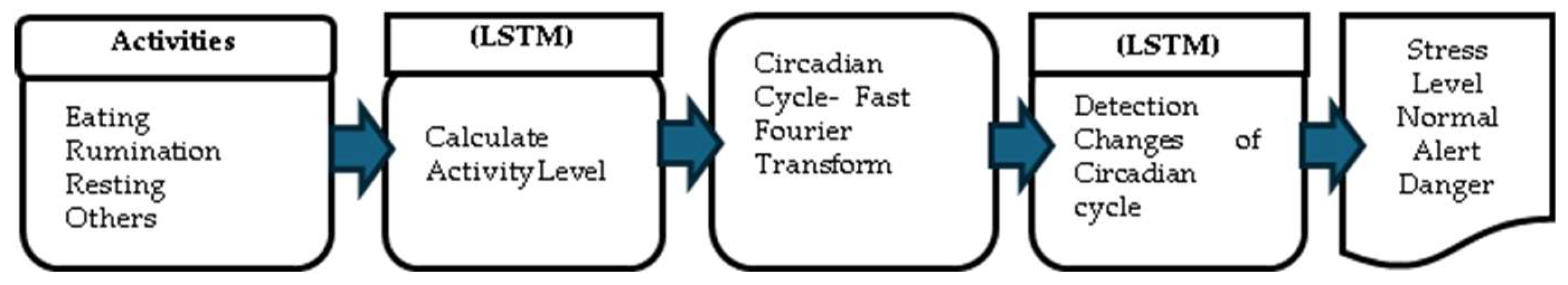
Figure 2.
Nedap SmartTag Collar Architecture.
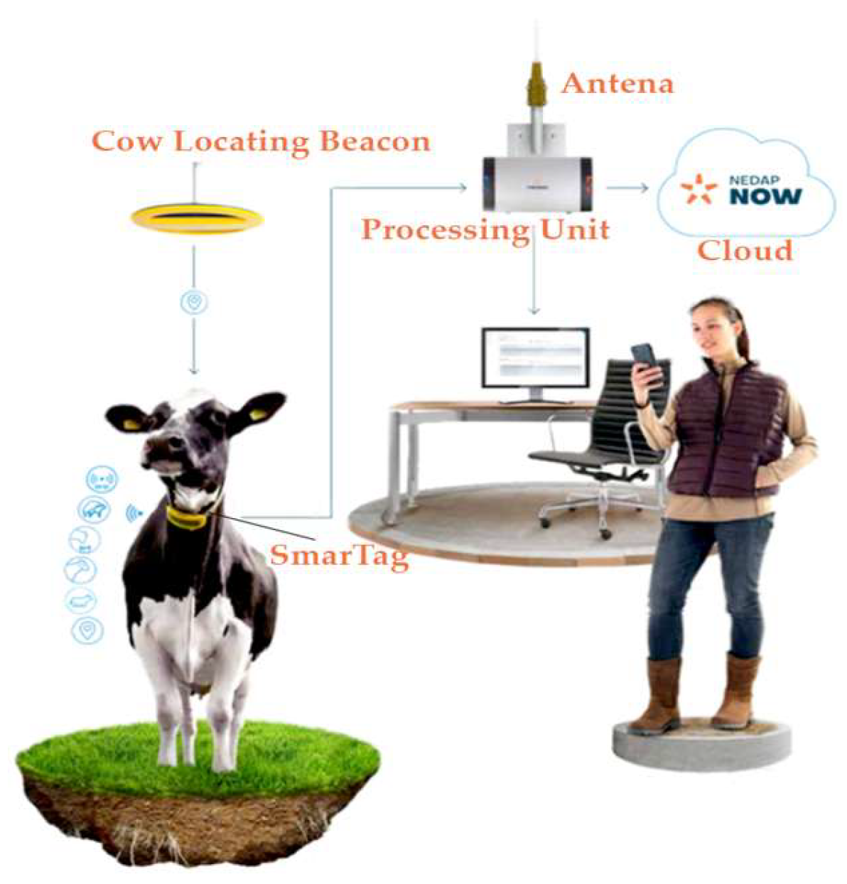
Figure 3.
Nedap system, collar monitoring.
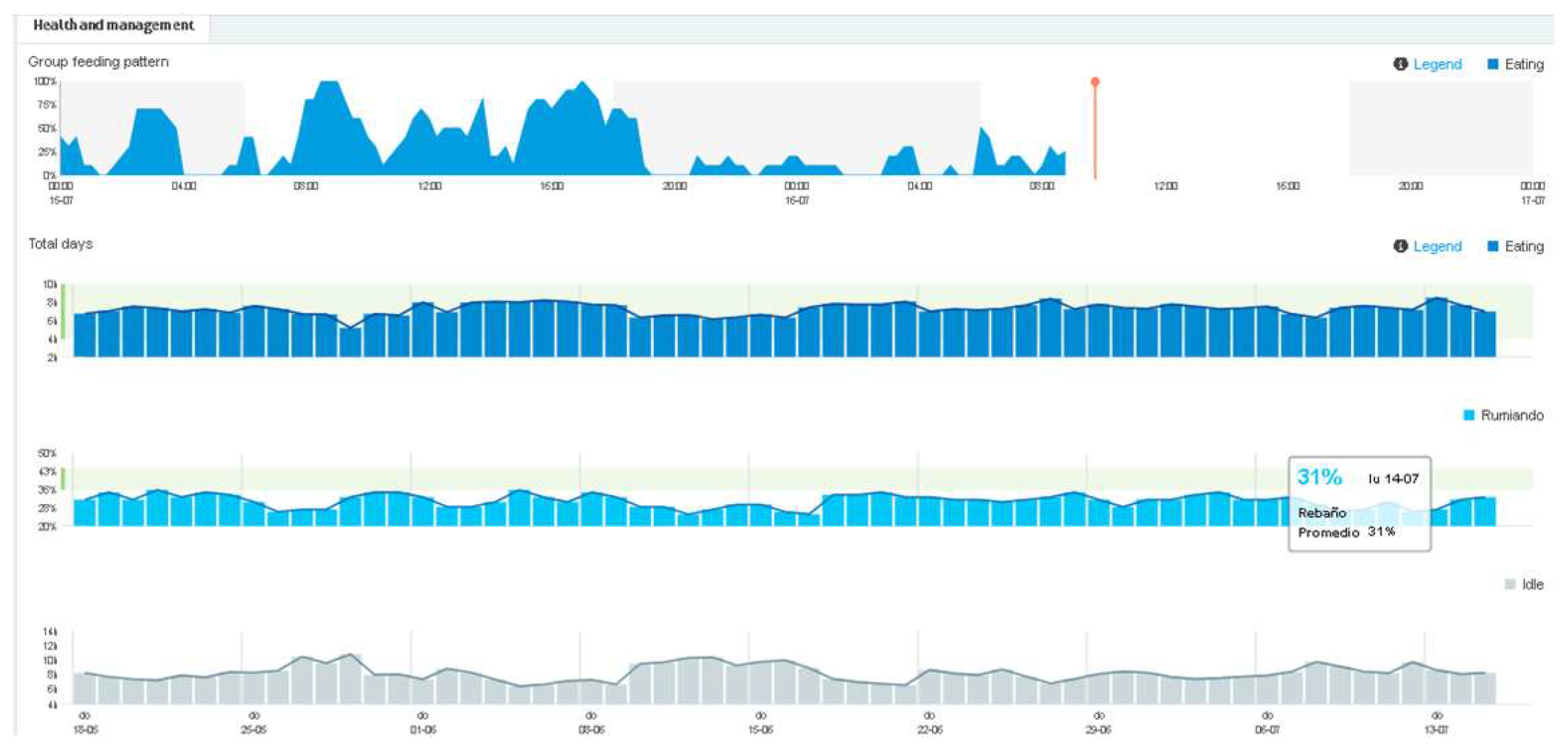
Figure 5.
Activity Level Monitoring and Prediction Model. https://proyectos.upec.edu.ec/ciclos/visualizacion email: revisor@upec.edu.ec password: revisor2025.
Figure 5.
Activity Level Monitoring and Prediction Model. https://proyectos.upec.edu.ec/ciclos/visualizacion email: revisor@upec.edu.ec password: revisor2025.
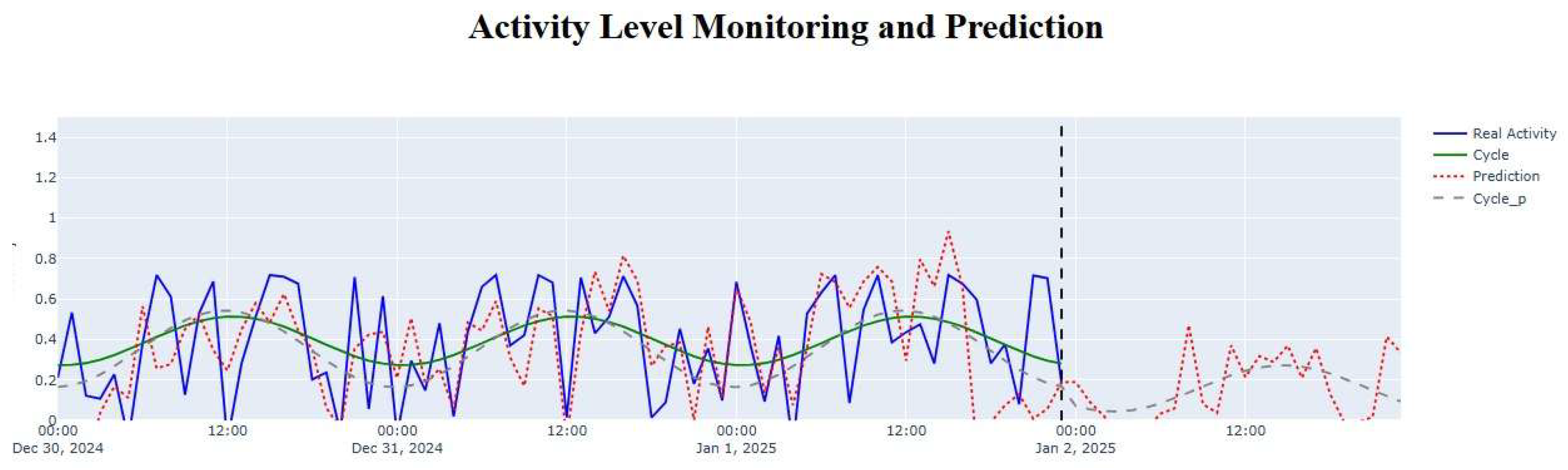
Table 1.
System components.
| Materials | Specifications |
|---|---|
|
Nedap Cow Control system |
Tool used to monitor cattle activity, collecting behavioral data. |
| Nedap SmartTag | Accelerometer-equipped collar for monitoring cattle activity. |
| Cattle | Holstein cows: 1.Cris, 2. Santa, 3. Luly, 4. Chela, 5. Joya, 6. Mishu, 7. Elyn, 8. Rosa, 9. Luna, 10. Kummy. |
| Circadian cycle extracted via Fourier Transform | Method used to analyze circadian patterns and classify stress levels into normal, alert, and danger categories. |
| Python | Programming language used for developing the predictive model and analyzing circadian data. |
| TensorFlow library | Tool used to implement and train the neural network model for stress prediction. |
| Visual Studio Code | Integrated Development Environment (IDE) used for writing and debugging project code. |
Disclaimer/Publisher’s Note: The statements, opinions and data contained in all publications are solely those of the individual author(s) and contributor(s) and not of MDPI and/or the editor(s). MDPI and/or the editor(s) disclaim responsibility for any injury to people or property resulting from any ideas, methods, instructions or products referred to in the content. |
© 2025 by the authors. Licensee MDPI, Basel, Switzerland. This article is an open access article distributed under the terms and conditions of the Creative Commons Attribution (CC BY) license (http://creativecommons.org/licenses/by/4.0/).
Copyright: This open access article is published under a Creative Commons CC BY 4.0 license, which permit the free download, distribution, and reuse, provided that the author and preprint are cited in any reuse.


