
Submitted:
31 July 2025
Posted:
06 August 2025
You are already at the latest version
Abstract
Our goal is to generate restructuring recommendations for research software systems based on software architecture descriptions that were obtained via reverse engineering. We reconstructed these software architectures via static and dynamic analysis methods in the reverse engineering process. To do this, we combined static and dynamic analysis for call relationships and dataflow into a hierarchy of six analysis methods. For generating optimal restructuring recommendations, we use genetic algorithms, which optimize the module structure. For optimizing the modularization, we use coupling and cohesion metrics as fitness functions. In general, our results confirm the applicability of genetic algorithms for optimizing the module structure of research software. Our experiments show that the analysis methods have a significant impact on the optimization results. A specific observation from our experiments is that the pure dynamic analysis produces significantly better modularizations than the optimizations based on the other analysis methods that we used for reverse engineering. Furthermore, a guided, interactive optimization with domain expert's feedback improves the modularization recommendations considerably.
Keywords:
software remodularization
; genetic optimization
; dynamic analysis
; static analysis
; research software
1. Introduction
Remodularization refers to the process of reorganizing or restructuring the modular components of a software system [1]. This is typically done to improve code quality, maintainability, scalability, or to better align with evolving requirements. Remodularization involves changing the way a software system is divided into modules. This could include splitting large modules into smaller, more cohesive ones; merging modules that are tightly coupled; or reassigning responsibilities among modules to reduce dependencies. To improve maintainability (easier to understand, test, and modify parts of the software system), enhance modularity (reduce coupling and increase cohesion), better adapt to change (support new features), or reduce technical debt (clean up legacy structures that no longer make sense), we optimize the module structure. Such an optimization is a recommendation for remodularization, whereby we do not change the semantics of the software.
We employ genetic algorithms for multi-objective optimization of module structures. The optimized objectives are low coupling and high cohesion. Thus, these metrics for coupling and cohesion are used as fitness functions in the genetic algorithm. We use six different analysis methods to compute these metrics based on the previous static and dynamic analysis of the existing software for reconstructing their software architecture. We analyze and discuss the impact of these analysis methods on the optimization results. Our specific application domain is research software [2], particularly earth system models (ESMs).
As contributions of this paper we provide:
- Based on the recovered software architectures of existing research software [3], we show that genetic algorithms allow to generate recommendations for restructuring this research software.
- To evaluate these recommendations for restructuring the ESMs, we collected feedback from domain experts who are involved in climate research as research software engineers. This feedback is also used for a guided, interactive optimization process.
In Section 2, we start with a look at the specific requirements of our application domain, which are the earth system models MITgcm and UVic. Then, we describe the reverse engineering process for architecture recovery in Section 3, which we applied as previous work [3] to MITgcm and UVic. Our genetic optimization process to generate restructuring recommendations is introduced in Section 4. The optimizations of MITgcm and UVic are presented in Section 5 and Section 6, respectively. We discuss our results in Section 7 and related work in Section 8, before we conclude the paper in Section 9 with an outlook to future work.
2. Our Application Domain: Earth System Models
Research software is software that is designed and developed to support research activities. It can be used to collect, process, analyze, and visualize data, as well as to model complex phenomena and run sophisticated simulations. Research software engineering research aims at understanding and improving how software is developed for research [2]. Various categories of research software exist. Category 1.1 of [6] describes “Modeling and Simulation” as a role for research software. Such simulation software is usually continually modified and enhanced to provide new insights for specific research questions.
Earth system models (ESMs) are such complex software systems used to simulate the earth’s climate and understand its effects on, e.g., oceans, agriculture, and habitats. They comprise different sub-models addressing specific aspects of the earth system, such as ocean circulation. Their code is, partly, decades old. Such scientific models can start as small software systems, which often evolve into large, complex models or are integrated into other models. Software engineering for such scientific models has specific characteristics [7], and involves dedicated roles such as model developers and research software engineers [8].
We chose UVic and MITgcm for our analysis, as they are used in many climate research projects, such as SOLAS [9], PalMod [10,11], CMIP6 [12], and the IPCC report [13]. Both ESMs are implemented in Fortran, run on Unix workstations without specific hardware requirements, and we collaborate with domain experts working with both models as research software engineers. MITgcm is referred to by the domain experts collaborating with us as a good example of a modern ESM, while UVic is a representative of a more traditionally developed ESM, whose development began in the 1960s.
A note on the term ‘model’ in climate science: In software engineering and information systems research, modeling is also an essential activity. Conversely to climate science, where climate models are the software systems to simulate the Earth, in software engineering and in information systems research, models are built as abstractions of the software systems themselves. A software architecture description is an example of such a model in software engineering [14], not to be confused with a (software) model of the Earth.
The ESMs are continually modified and enhanced to provide new insights for specific research questions. This leads to numerous variants and versions for an ESM which must be maintained as other scientists intend to base their research on new features and reproduce results. Thus, ESMs are long-living software [15], and face typical risks, e.g., blurring module boundaries and architectural erosion, due to changes in functionality, hardware and language features. The resulting architectural debts [16] can limit further research and may harm the validity of scientific results. Furthermore, the lack of documentation and the loss of knowledge, as scientists move to other positions, limit the maintainability of ESMs. Therefore, the long-term development of ESMs faces unique challenges. Our goal is to determine how software engineering techniques and tools that have been successfully applied in other areas can assist in the development of ESMs.
To ensure the maintainability of ESMs, an understanding of the software architecture is necessary [17]. Documentation is usually rare in this domain. In particular, architecture documentation is, if it exists at all, often outdated and incomplete. Thus, rediscovering the architecture of ESMs is a key step to ensure their longevity, as it allows guiding architecture improvements and to identify areas that should be restructured. Architectural analyses provide an overview of the ESM’s structure and dependencies. They allow to identify interfaces that support developers in extending a model or adding alternative sub-models to an ESM. In addition, they help new scientists understand the model implementation. Furthermore, based on structural optimizations, developers can improve the architecture over time to facilitate future developments.
Thus, reconstructing the architecture of the simulation software via reverse engineering (see Section 3) is a key step to ensure its longevity, as it is a basis for guiding architecture improvements and identifying areas that should be restructured.
3. Reverse Engineering the Software Architecture
A prerequisite for a structural software optimization is the availability of a software architecture description of the existing software. So, the first step is to reconstruct the software architecture of the software via reverse engineering, which can then be optimized. Here, we briefly summarize the relevant parts of our analysis approach, the full approach is detailed in [3]. Our analysis takes static and dynamic analysis, control flow and data flow into account to construct the required software architecture descriptions. Figure 1 presents an overview of our reverse engineering process.
We combine static and dynamic analysis techniques. Our analysis process can be configured to take any combination of static method-call analysis, dynamic method-call analysis, or static dataflow analysis into account, by merging the results of the individual analyses (this is the Combine Architectures step of Figure 1).
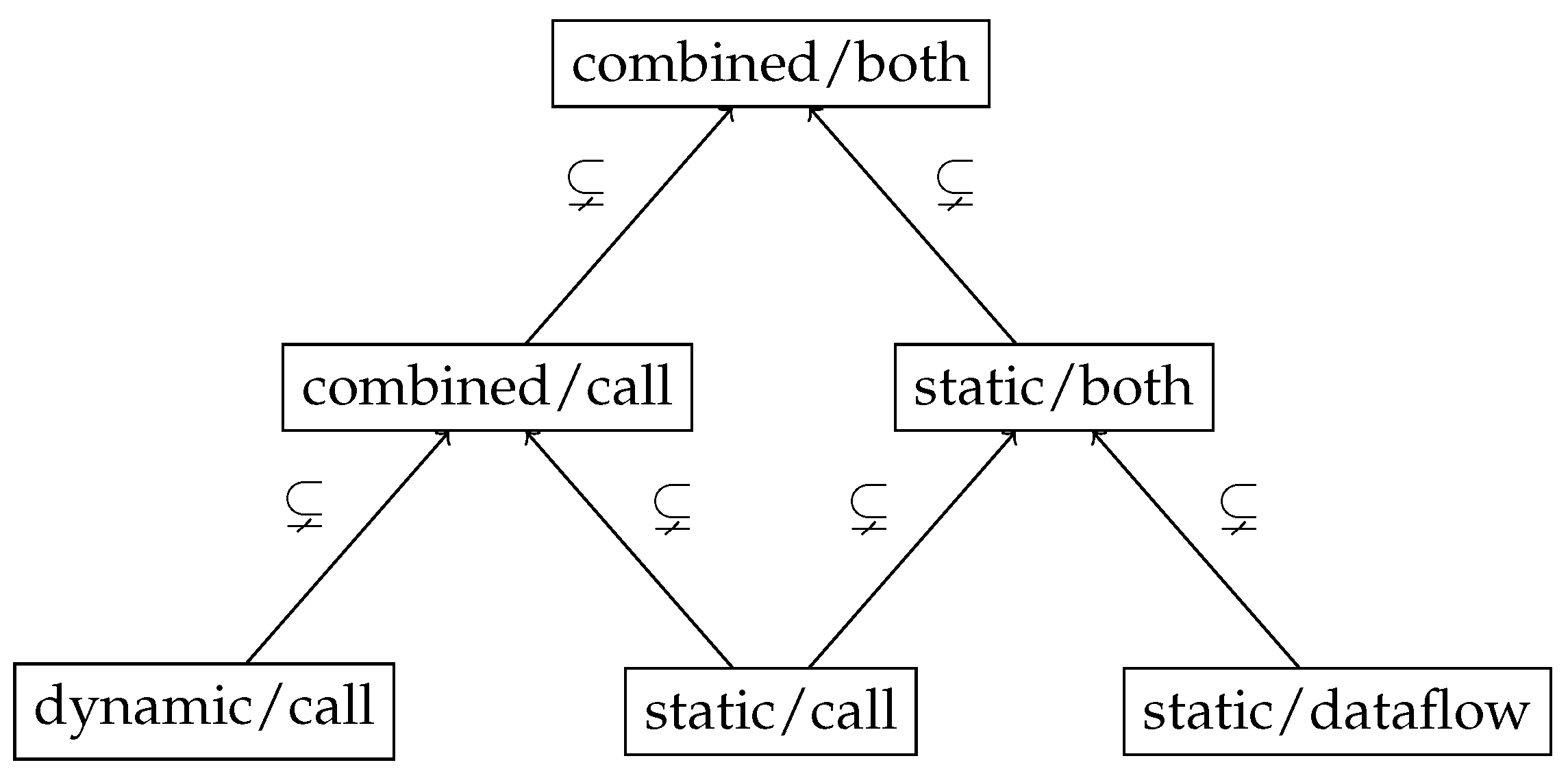
We categorize these methods into six different analysis methods, displayed in Figure 2. These methods form a hierarchy, e.g., the analysis method combined/call is obtained by merging the results of dynamic/call (only dynamic analysis) and static/call (only static analysis). The method static/both is obtained by merging the results of static/call and static/dataflow. At the top, all methods are combined into combined/both.
Figure 2.
Hierarchy of our analysis methods. At the bottom, we analyze dynamic and static call-relationships, and static dataflows. Then, we combine the call and static methods.
Figure 2.
Hierarchy of our analysis methods. At the bottom, we analyze dynamic and static call-relationships, and static dataflows. Then, we combine the call and static methods.
The output of our analysis process, insofar as relevant for our optimization, is a coupling graph as software architecture description of the analyzed software: The nodes of this graph are the compilation units of the analyzed software and its edges are call- or dataflow relations: There is an edge between functions f and g if the function g is called from the function f, or if data flows from f to g (this can be by a parameter, a return value, or by shared access of global data).
Reverse engineering MITgcm and UVic revealed that the architecture of an ESM differs significantly from that of, e.g., web-based systems, where the differences between dynamic and static analyses are much more significant [18]. A possible reason for this is that the design of an ESM can anticipate the way the code will execute much better than the design of an event-based system, where much of the actual behavior depends on events that cannot be predicted at design time.
4. Genetic Optimization to Generate Restructuring Recommendations
The output of our optimization process are recommendations to improve the module structure of the existing software systems. In addition, the optimization process also provides the developers with an overview of both the optimization potential and the involved trade-offs between the modularization options. We describe our genetic optimization approach in Section 4.1. The specific fitness functions for optimizing the module structure are introduced in Section 4.2.
4.1. Genetic Algorithms for Multi-Objective Optimization
Genetic algorithms are inspired by biology, and use recombination, mutation, and selection based on fitness functions to approximate optimal solutions. Figure 3 illustrates our architecture optimization process. The recovered architecture from the preceding reverse engineering process is first restructured via recombination and mutation. The obtained restructured architectures are then selected based on the fitness functions. The process can be configured to run either for a specified period of time, for a fixed number of generations, until the involved metrics are below a given threshold, or until no significant progress is achieved anymore in each step (good enough). For the results in the present paper, we let each optimization run for maximally two hours.
Figure 3.
Our genetic architecture optimization process. The preceding reverse engineering process was illustrated in Figure 1 above. It provides us with the recovered architecture as input. The improvement recommendations are the output of our architecture optimization process.
Figure 3.
Our genetic architecture optimization process. The preceding reverse engineering process was illustrated in Figure 1 above. It provides us with the recovered architecture as input. The improvement recommendations are the output of our architecture optimization process.
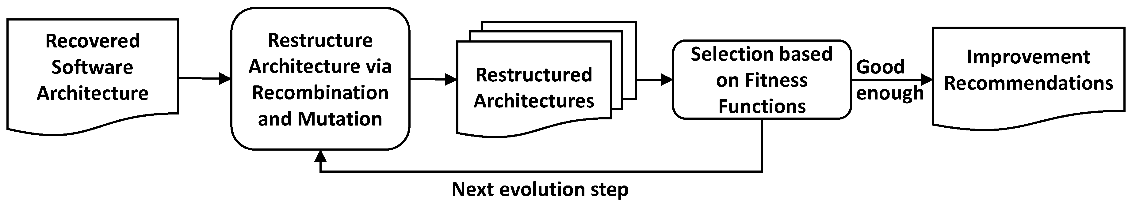
If one of these termination criteria is met, we generate improvement recommendations. Otherwise, we iterate with the next evolution step. We will start initially with unguided optimizations, and subsequently complement this with a guided, interactive optimization. This guided, interactive optimization takes expert feedback into account to restrict the search space. In our case, the fitness functions are the software quality metrics, which are introduced in the following subsection.
4.2. Software Quality Metrics as Fitness Functions
Our optimization process can be configured to use a wide range of different optimization metrics as fitness functions. For optimizing the modularization, we use coupling and cohesion metrics [1] to measure the quality of both the original software structure and the suggested optimizations. These metrics use the coupling graph, which is the output of our reverse engineering process (Section 3), to measure the fitness of the software’s modularization:
- StrCoup:
- Structural coupling is defined as the average in/out degree of components, i.e., the average number of edges connecting a program unit in the current component with a program unit in another component,
- LStrCoh:
- Lack of structural cohesion is defined as the average number of pairs of unrelated units in a component, i.e., the number of pairs where both u and v are program units, and there is no edge connecting u and v in the coupling graph.
Both of these metrics are chosen such that small values are better (as is usual in multi-objective optimization).
Obviously, there is a trade-off between coupling and cohesion, since one can easily reduce coupling by merging different components, which then often leads to less cohesive components (see Section 5.1 for examples). As usual when studying optimizations with multiple criteria, we call a modularization m undominated, if there is no other modularization that is strictly better than m with regard to one criterion (StrCoup or LStrCoh), and at least as good as m with respect to the other. There can be multiple undominated modularizations, the set of these is called the Pareto front. These modularizations represent an optimal trade-off between the involved metrics, in the sense that improving one metric is impossible without worsening the other metric. To compute an approximation of the Pareto front, we adapt the approach from Candela et al. [1] and apply the genetic algorithm NSGA-II [19].
5. Optimization of MITgcm Global Ocean
In the following, we compare optimizations of the MITgcm variant global-ocean-cs32x15 based on the different analysis techniques depicted in Figure 2. Results for other MITgcm variants can be found in the supplementary material [20]. Section Section 5.1 presents the results of our initial unguided optimization, and Section 5.2 the subsequent guided, interactive optimization.
5.1. Unguided Optimization
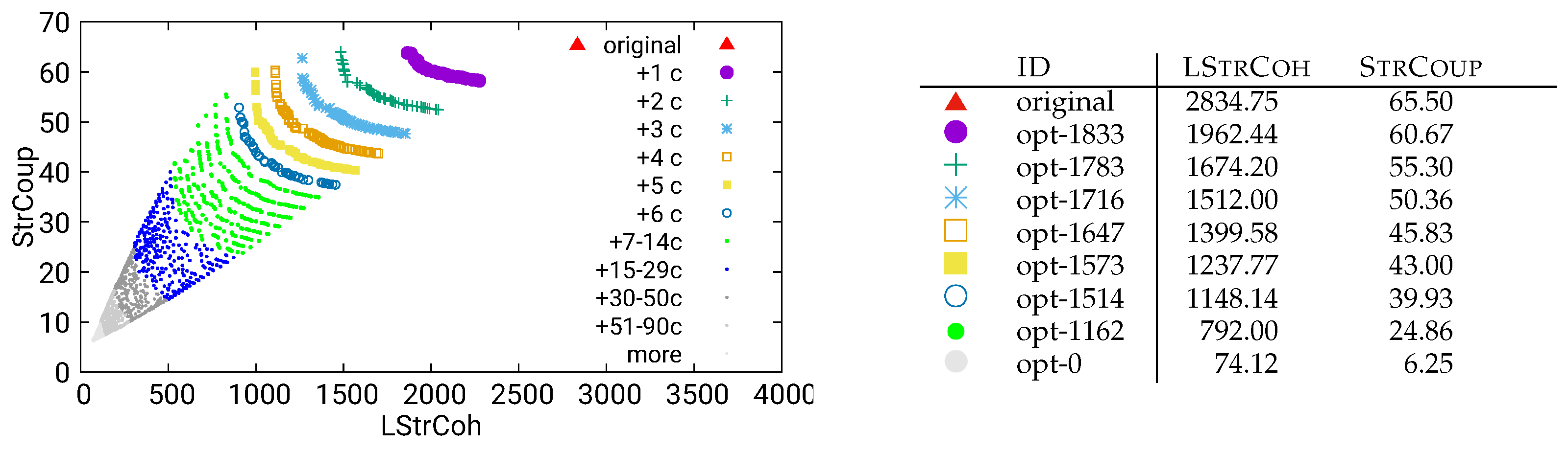
We present our first optimization result in Figure 4. This plot shows the result of running our genetic algorithm on the model obtained from the MITgcm variant global-ocean-cs32x15 by the dynamic/call analysis method. The result is a large set of new modularizations of the software. In the above plot, each modularization is represented as a dot expressing its StrCoup and LStrCoh values on the two axes. The original modularization is indicated by a red triangle  .
.
.In the table on the right-hand side of Figure 4, we present the values of our software quality metrics for some specifically chosen modularizations. Here, we can observe some “extreme” optimizations:
- The modularization opt-1238 achieves a coupling degree of zero, at the price of very low cohesion (recall that LStrCoh measures the lack of cohesion, so high values indicate low cohesion). Manual inspection of this modularization shows that opt-1238 merges components to obtain a modularization that consists of two unrelated components (and hence obtains coupling degree zero).
- An even more extreme modularization is opt-1260, which merges all components into a single one–with the “benefit” of fewer components, but at the price of a very low cohesion.
- A third “extreme” modularization is opt-180, which achieves full cohesion (i.e., zero lack of cohesion) while still improving the coupling value over the original modularization (1.72 instead of 2.84). However, a manual inspection of this solution shows that it distributes 96 units into 83 components, which are then mostly one-element components. Such components are cohesive, but obviously this is not a good way to structure a software system.
Obviously, modularizations such as the extreme ones opt-180, opt-1238, and opt-1260 are not our goal. More generally, optimizations that, compared to the original modularization, improve one of the two quality metrics (LStrCoh or StrCoup) and worsen the other are usually not relevant for practice. Therefore, we will now only consider optimization results that improve over the original modularization with regard to both StrCoup and LStrCoh, and focus on the solutions that only modestly increase the number of components.
In order to focus on modularizations that only use a reasonable number of components, we use larger and more colorful symbols for solutions introducing few additional components, and smaller, less colorful dots for solutions introducing many components (this is better visible in Figure 5, which zooms into the part of Figure 4 that contains the most relevant optimizations). As an example, results shown with a purple circle  denote optimization results that introduce at most a single additional component compared to the original modularization of the software, while blue star-shaped symbols
  represent results that introduce three additional components, and the small blue dot
  stands for optimizations introducing at least 15 and at most 29 additional components (the complete list of symbols is given in the legend of the plots). In this way, the plots illustrate not only the (expected) tradeoff between the quality metrics LStrCoh and StrCoup, but also between the conflicting goals of improving these metrics and introducing a few new components.
denote optimization results that introduce at most a single additional component compared to the original modularization of the software, while blue star-shaped symbols represent results that introduce three additional components, and the small blue dot stands for optimizations introducing at least 15 and at most 29 additional components (the complete list of symbols is given in the legend of the plots). In this way, the plots illustrate not only the (expected) tradeoff between the quality metrics LStrCoh and StrCoup, but also between the conflicting goals of improving these metrics and introducing a few new components.As discussed above, the optimizations in Figure 5 contain many promising suggestions, an example is opt-467, which improves on both quality metrics compared to the original modularization (LStrCoh decreases from 68 to ; StrCoup decreases from to ) while introducing only a single additional component. In order to study the effect of the choice of the analysis method (see Figure 2) on the quality of the obtained optimizations, we also performed optimizations based on the other five analysis methods.
We start, in Figure 6, with the analysis method combined/both, i.e., the method taking all available data (both static and dynamic analysis, both call and dataflow relationships) into account. It is obvious from Figure 6 that the optimization results are of a much lower quality than the ones obtained from our dynamic-only analysis (Figure 5 above): All results that actually improve on the original modularization introduce many additional components, whereas Figure 5 shows many relevant improvements introducing only a single component (represented by the large purple dots).
So, comparing the two optimization runs using dynamic/call (Figure 5) and combined/both (Figure 6), the two figures look very different, with the former yielding much more satifsfying results. To investigate the reason for these differences, we performed similar optimization runs with the remaining four analysis methods. Out of the three “base” methods (i.e., the lowest three in the presentation from Figure 2), the method static/dataflow is conceptually most different from dynamic/call, since it uses static instead of dynamic data, and dataflow instead of method-call relationships. We present the results of the corresponding optimization in Figure 7. It is obvous that the optimizations obtained from this method are problematic in the same way as those obtained from the combined/both method (Figure 6): There are again very few modularizations that improve on both our quality metrics without introducing many new components.
The third “base” analysis method from Figure 2 is static/call, which uses method-call relationships (as dynamic/call) based on static code analysis (as static/dataflow). The optimization results can be found in Figure 8. It is obvious that these results again share the same problems as the ones presented in Figure 6 and Figure 7, with no modularizations that significantly improve our quality metrics without introducing too many new components.
The two second-level analysis methods from Figure 2 lead to similar results, and can be found in Figure 9 for static/both and in Figure 10 for combined/call.
As a consequence of our analysis of the optimization runs based on our six different analysis methods, it is obvious that the dynamic-only analysis dynamic/call stands out—it contains many more “interesting” optimization results, i.e., ones that are both an improvement over the original modularization and also do not add too many new components to the software. There are some differences between the modularizations based on the other five analysis types, but none of them yields improvements like dynamic/call.
5.2. Guided, Interactive Optimization
The optimizations reported on in the preceding Section 5.1 took the entire model of the software (e.g., the MITgcm variant under analysis) into account and attempt to obtain a new global structure for the software. However, as confirmed in our discussion with ESM developers, applying the result of such a global optimization to a software system with a long development history and a large number of developers is not realistic. The ocean scientists were much more interested in more “local” optimizations, where the goal is not to find a completely new structure for the entire software, but to decompose an existing component into very few (ideally only two) new components.
To address this, we used our optimization software to decompose a single component (for MITgcm, the ‘src’ component was suggested to us as a realistic target, for UVic, the ‘common’ component plays a similar role). In the following, we present the results of these guided, interactive optimizations for the two analysis methods dynamic/call (Figure 11) and combined/both (Figure 12). The results for the remaining four analysis methods can be found in Figure 13, Figure 14, Figure 15 and Figure 16.
Since the optimization now only changes a single component, the search space and the optimization potential are very restricted. Surprisingly, this restricted search space leads to much better optimizations than the unguided optimizations reported in Section 5.1.
It is again obvious that the dynamic-only analysis dynamic/call stands out: The plot is much more sparsely populated than the other ones, i.e., the algorithm found fewer improvements here than for the other analysis methods. This is not surprising, since the number of units found in the src component is much smaller compared to the other analysis methods. The dynamic-only analysis found 51 units in the selected ‘src’ component, while the other analysis found between 371 and 393 units (see [3] for more details). Therefore, the search space for the dynamic-only analysis was much smaller than for the other analysis types.
The difference between the other five analysis techniques is again smaller than the difference between the dynamic-only analysis and the other five ones.
Another interesting observation is that results for our guided, interactive optimization are, in parts, even better than the results for the global optimization: Comparing, e.g., Figure 6 and Figure 12 (both using the static/call analysis method): The numerically best optimization opt-0 has almost the same StrCoup value ( vs ) in both results, but the single-component optimization has a much better LStrCoh value ( vs ). The best “single added component” optimization has both a better StrCoup value ( vs ), and a better LStrCoh value ( vs. ) in the local optimization. The results are similar when comparing other lines in the corresponding tables: Even though the one-component optimization has a severely restricted search space, the optimization results are not clearly inferior to those of the global optimization problem.
A possible reason for this is that with the smaller search space, the algorithm can find the optimal values in this restricted space sooner. To test this hypothesis, we also let one global optimization problem run for a longer time (24 hours instead of the 2 hours for the other optimization runs). The result is presented in Figure 17 and shows that the optimal solution with respect to both StrCoup and LStrCoh (opt-0) is in fact much better with regard to both metrics than the shorter runs reported in Figure 6 and Figure 12.
6. Optimization of UVic
As a comparison to the MITgcm ESM studied above, we also applied our methods to the UVic ESM. Similarly to MITgcm above, we first performed an unguided optimization, taking the entire ESM into account (Section 6.1), and then, based on feedback from modelers, restricted our optimizations to the common component (6.2). The results are similar to those for MITgcm presented above, we therefore keep the presentation short and highlight the differences. Again, Section 6.1 presents the results of our initial unguided optimization, and Section 6.2 the subsequent guided, interactive optimization.
6.1. Unguided Optimization
We present the optimization runs based on the two most “extreme” analysis methods, taking the least (dynamic/call, Figure 18) and the most (combined/both, Figure 19) information into account. The results of the other four analysis methods can be found in Figure 20, Figure 21, Figure 22 and Figure 23.
It is obvious that the differences between these two optimization runs are much smaller than between the corresponding methods in the MITgcm case, and that both optimizations suffer from the same problem as most of our optimizations of MITgcm: There are hardly any optimizations that improve both our quality metrics and do not add too many new components. The difference to the MITgcm case is that the optimization run based on dynamic/call in Figure 18 does not stand out as much against the other runs here as was the case for MITgcm. The reason for this is that, as discussed in [3], our dynamic analysis of UVic yielded a much more complete architecture model than that of MITgcm.
6.2. Guided, Interactive Optimization
Restricting the optimizations again to a single component of UVic has similar effects as in the case of MITgcm: The search space for the optimizations is very restricted, resulting in quite similar results for the different analysis techniques. We present the optimizations based on our different analyses techniques in Figure 24, Figure 25, Figure 26, Figure 27, Figure 28 and Figure 29.
7. Discussion
In general, our results confirm the applicability of genetic algorithms for optimizing the module structure of ESMs. We can draw two main observations from our experiments:
- The pure dynamic analysis produces significantly better modularizations than the optimizations based on the other analysis methods that we used for reverse engineering. This may a specific observation for our application domain of research software: If we use the scientific model for a specific experiment, we can optimize the software architecture for this specific use case. Only those parts of the software that are actually used in the experiment are represented in the reconstructed architecture, which is then optimized.
- The guided, interactive optimization provides good modularizations. Thus, we can recommend to feed expert feedback into the optimization process.
We also observed differences between our example systems, MITgcm and Uvic. As demonstrated by the analysis, the existing legacy modularization of UVic is very poor with respect to the metrics LStrCoh and StrCoup. This coincides with the experience communicated by UVic developers.
For domain experts, support for program comprehension was another key takeaway, in addition to the restructuring recommendations. They found program comprehension helpful for their daily work, especially connecting the interface descriptions with the code base. From our discussions with the domain experts, we also obtained suggestions for other ESMs on which to apply our methods. This will be an area for future work.
8. Related Work
Praditwong et al. [21] investigated the application of multi-objective genetic algorithms to software restructuring. Mkaouer et al. [22] also applied genetic algorithms, with the additional goal of minimizing the resulting changes to the considered software. To the best of our knowledge, we are the first to apply genetic algorithms for restructuring ESMs. Sudhakar and Nithiyanandam [23] use clustering algorithms like K-Means and MAD-ENRNN to restructure object-oriented software. Maikantis et al. [24] also use genetic algorithms for restructuring software. As far as we know, our paper is the first one to compare optimizations obtained by dynamic and static analysis techniques.
Cortellessa et al. [25] employ genetic algorithms to optimize software architectures with respect to performance and reliability, while we optimize the module structures with respect to cohesion and coupling. Similar to our work, they integrate interaction with engineers into the optimization process.
Pourasghar et al. [26] also employ genetic algorithms to optimize module structures with respect to cohesion and coupling. Different to our approach, they integrate control flow into their software analysis, while we integrate data flow in software modularization.
9. Conclusions and Future Work
We applied our architecture optimizations to the ESMs UVic and MITgcm. The optimizations computed significant numerical improvements for restructuring recommendations for both ESMs. The pure dynamic analysis produces significantly better modularizations. In particular, guided, interactive optimization, such as restricting to a single component, helps to get better results. In addition to the actual optimization results, getting an overview about the optimization potential is very helpful for the developers.
In the future, we plan to take into account additional information for our optimization recommendations. Our analysis so far was based on calls and dataflow relationships between operations. However, there are additional dependencies that we can utilize. One example for this is semantic coupling, which measures the similarity of e.g., operation names. If the software under analysis uses a well-designed naming scheme, it can be beneficial to keep operations with similar names (or common prefixes in the names) in the same components. We implemented such a metric (using the edit distance from Levenshtein [27]) and used it to enrich the coupling graph with additional edges reflecting common prefixes of method names. First results indicate that this method is more beneficial for MITgcm than for UVic, possibly indicating that the former’s naming scheme for operations is more helpful for optimization. A preliminary take-away is that metrics beyond the standard coupling and cohesion metrics should be chosen very carefully, and this choice must take knowledge of the structure and possibly the development conventions (such as naming schemes) of the examined software into account. Other metrics that we plan to evaluate are test metrics discussed in [28] and clustering metrics from [29], which we anticipate can be used both in optimization and in interface discovery.
Author Contributions
Conceptualization, H.S., W.H. and R.J.; methodology, H.S., W.H. and R.J.; software, H.S.; validation, H.S., W.H. and R.J.; investigation, H.S.; writing—original draft preparation, H.S., W.H. and R.J.; writing—review and editing, H.S., W.H. and R.J.; visualization, H.S., W.H. and R.J.; funding acquisition, W.H. All authors have read and agreed to the published version of the manuscript.
Funding
This work was funded by the Deutsche Forschungsgemeinschaft (DFG, German Research Foundation), grant no. HA 2038/8-1—425916241.
Institutional Review Board Statement
Not applicable.
Informed Consent Statement
Not applicable.
Data Availability Statement
We provide a replication package for the architecture optimizations [20]. This package contains detailed instructions on running our re-modularization algorithms. A Docker file allows to run the analyses without manually installing the required software. Additional optimization results can be found in the contained file complete-analysis-results.pdf.
Conflicts of Interest
The authors declare no conflicts of interest.
Abbreviations
The following abbreviations are used in this manuscript:
| CMIP | Coupled Model Intercomparison Project |
| ESM | Earth System Model |
| IPCC | Intergovernmental Panel on Climate Change |
| LStrCoh | Lack of Structural Cohesion |
| MITgcm | MIT General Circulation Model |
| NSGA | Non-dominated Sorting Genetic Algorithm |
| PalMod | Paleoclimatic Modeling |
| SOLAS | Surface Ocean-Lower Atmosphere Study |
| StrCoup | Structural Coupling |
| UVic | University of Victoria Earth System Climate Model |
References
- Candela, I.; Bavota, G.; Russo, B.; Oliveto, R. Using Cohesion and Coupling for Software Remodularization: Is It Enough? ACM Trans. Softw. Eng. Methodol. 2016, 25, 24:1–24:28. [CrossRef]
- Felderer, M.; Goedicke, M.; Grunske, L.; Hasselbring, W.; Lamprecht, A.L.; Rumpe, B. Investigating Research Software Engineering: Toward RSE Research. Commun. ACM 2025, 68, 20–23. [CrossRef]
- Hasselbring, W.; Jung, R.; Schnoor, H. Software Architecture Evaluation of Earth System Models. J. Softw. Eng. Appl. 2025, 18, 113–138. [CrossRef]
- Weaver, A.J.; et al. The UVic earth system climate model: Model description, climatology, and applications to past, present and future climates. Atmos. Ocean 2001, 39, 361–428. [CrossRef]
- Artale, V.; et al. An atmosphere-ocean regional climate model for the Mediterranean area: assessment of a present climate simulation. Clim. Dyn. 2010, 35, 721–740. [CrossRef]
- Hasselbring, W.; Druskat, S.; Bernoth, J.; Betker, P.; Felderer, M.; Ferenz, S.; Hermann, B.; Lamprecht, A.L.; Linxweiler, J.; Prat, A.; et al. Multi-Dimensional Research Software Categorization. Computing in Science & Engineering 2025, pp. 1–10. [CrossRef]
- Johanson, A.; Hasselbring, W. Software Engineering for Computational Science: Past, Present, Future. Comput. Sci. Eng. 2018, 20, 90–109. [CrossRef]
- Jung, R.; Gundlach, S.; Hasselbring, W. Software Development Processes in Ocean System Modeling. Int. J. Model. Simulation, Sci. Comput. 2022, 13, 2230002. [CrossRef]
- Bréviére, E.H.; et al. Surface ocean-lower atmosphere study: Scientific synthesis and contribution to Earth system science. Anthropocene 2015, 12, 54–68. [CrossRef]
- Pahlow, M.; Chien, C.T.; Arteaga, L.A.; Oschlies, A. Optimality-based non-Redfield plankton–ecosystem model (OPEM v1. 1) in UVic-ESCM 2.9–Part 1: Implementation and model behaviour. Geosci. Model Dev. 2020, 13, 4663–4690. [CrossRef]
- Chien, C.T.; Pahlow, M.; Schartau, M.; Oschlies, A. Optimality-based non-Redfield plankton–ecosystem model (OPEM v1. 1) in UVic-ESCM 2.9–Part 2: Sensitivity analysis and model calibration. Geosci. Model Dev. 2020, 13, 4691–4712. [CrossRef]
- Mengis, N.; et al. Evaluation of the University of Victoria Earth System Climate Model version 2.10 (UVic ESCM 2.10). Geosci. Model Dev. 2020, 13, 4183–4204. [CrossRef]
- Stocker, T.F.; et al. Climate Change 2013 – The Physical Science Basis: Working Group I Contribution to the Fifth Assessment Report of the Intergovernmental Panel on Climate Change; Cambridge University Press, 2014. [CrossRef]
- Hasselbring, W. Software Architecture: Past, Present, Future. In The Essence of Software Engineering; Springer International Publishing: Cham, 2018; pp. 169–184. [CrossRef]
- Reussner, R.; Goedicke, M.; Hasselbring, W.; Vogel-Heuser, B.; Keim, J.; Märtin, L. Managed Software Evolution; Springer: Cham, 2019. [CrossRef]
- Verdecchia, R.; Kruchten, P.; Lago, P., Architectural Technical Debt: A Grounded Theory. In Software Architecture; Springer, 2020; pp. 202––219. [CrossRef]
- Druskat, S.; Eisty, N.U.; Chisholm, R.; Chue Hong, N.; Cocking, R.C.; Cohen, M.B.; Felderer, M.; Grunske, L.; Harris, S.A.; Hasselbring, W.; et al. Better Architecture, Better Software, Better Research. Comput. Sci. Eng. 2025, pp. 1–11. [CrossRef]
- Schnoor, H.; Hasselbring, W. Comparing Static and Dynamic Weighted Software Coupling Metrics. Computers 2020, 9, 24. [CrossRef]
- Deb, K.; Pratap, A.; Agarwal, S.; Meyarivan, T. A fast and elitist multiobjective genetic algorithm: NSGA-II. IEEE Trans. Evol. Comput. 2002, 6, 182–197. [CrossRef]
- Jung, R.; Schnoor, H.; Hasselbring, W. Replication Package for: Software Architecture Evaluation of Earth System Models (Restructuring Part), 2025. [CrossRef]
- Praditwong, K.; Harman, M.; Yao, X. Software Module Clustering as a Multi-Objective Search Problem. IEEE Trans. Softw. Eng. 2011, 37, 264–282. [CrossRef]
- Mkaouer, W.; Kessentini, M.; Shaout, A.; Koligheu, P.; Bechikh, S.; Deb, K.; Ouni, A. Many-objective software remodularization using NSGA-III. ACM Trans. Softw. Eng. Methodol. (TOSEM) 2015, 24, 1–45. [CrossRef]
- Sudhakar, G.; Nithiyanandam, S. DOOSRA—Distributed Object-Oriented Software Restructuring Approach using DIM-K-means and MAD-based ENRNN classifier. IET Softw. 2023, 17, 23–36. [CrossRef]
- Maikantis, T.; Tsintzira, A.A.; Ampatzoglou, A.; Arvanitou, E.M.; Chatzigeorgiou, A.; Stamelos, I.; Bibi, S.; Deligiannis, I. Software architecture reconstruction via a genetic algorithm: Applying the move class refactoring. In Proceedings of the 24th Pan-Hellenic Conference on Informatics, 2020, pp. 135–139. [CrossRef]
- Cortellessa, V.; Diaz-Pace, J.A.; Di Pompeo, D.; Frank, S.; Jamshidi, P.; Tucci, M.; van Hoorn, A. Introducing Interactions in Multi-Objective Optimization of Software Architectures. ACM Trans. Softw. Eng. Methodol. 2025, 34, 1–39. [CrossRef]
- Pourasghar, B.; Izadkhah, H.; Akhtari, M. Beyond Cohesion and Coupling: Integrating Control Flow in Software Modularization Process for Better Code Comprehensibility. ACM Trans. Softw. Eng. Methodol. 2025, 34, 1–29. [CrossRef]
- Levenshtein, V.I. Binary codes capable of correcting deletions, insertions and reversals. Soviet Physics Doklady. 1966, 10, 707–710.
- Ankerst, M.; Breunig, M.M.; Kriegel, H.P.; Sander, J. OPTICS: ordering points to identify the clustering structure. SIGMOD Rec. 1999, 28, 49–60. [CrossRef]
- Navarro, G. A guided tour to approximate string matching. ACM Comput. Surv. 2001, 33, 31–88. [CrossRef]
Figure 1.
Our reverse engineering process [3]. First, our tools recover the architecture via reverse engineering with dynamic and static analysis. Then, the results of dynamic and static analysis are combined. The recovered software architecture is used as input for the subsequent optimization process, which will be introduced in Section 4 with Figure 3 below.
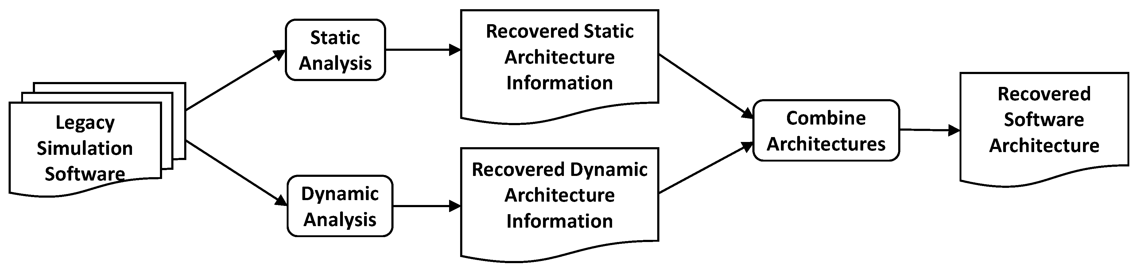
Figure 4.
Unguided optimization of MITgcm (global-ocean-cs32x15) using dynamic/call data
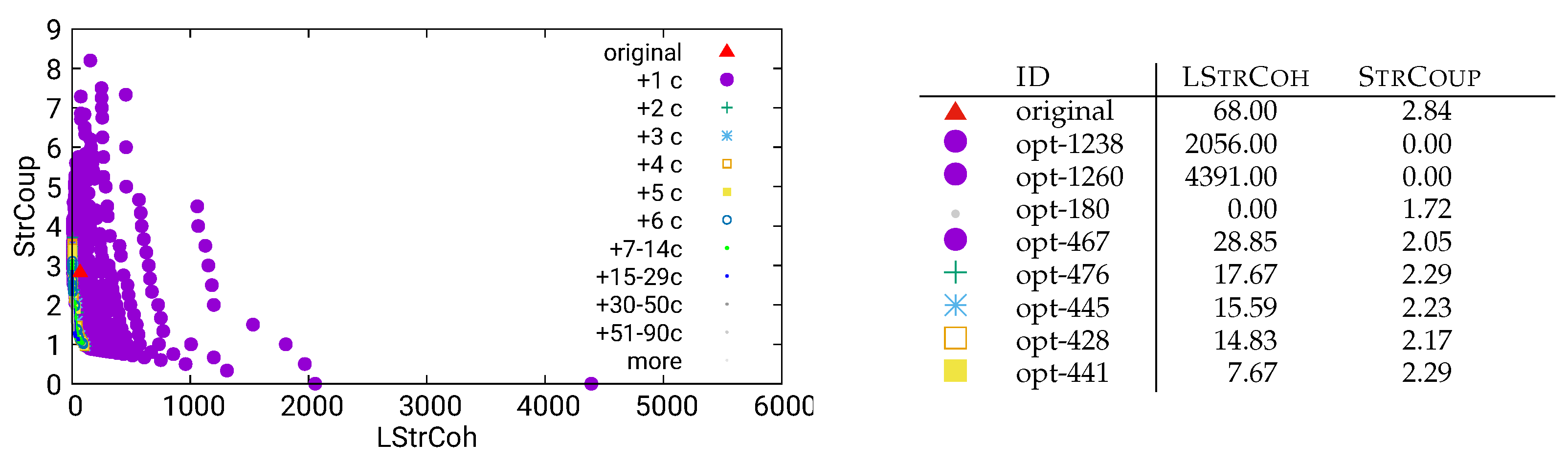
Figure 5.
Zoom into the part of Figure 4 that contains the most relevant optimizations
Figure 5.
Zoom into the part of Figure 4 that contains the most relevant optimizations
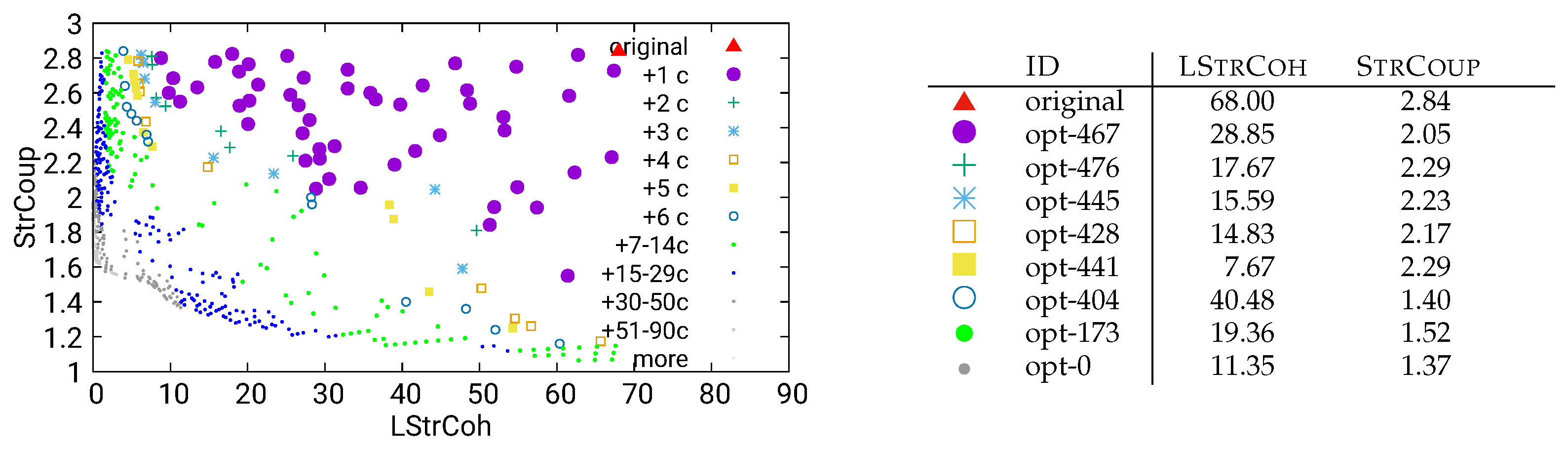
Figure 6.
Unguided of MITgcm (global-ocean-cs32x15) using combined/both data
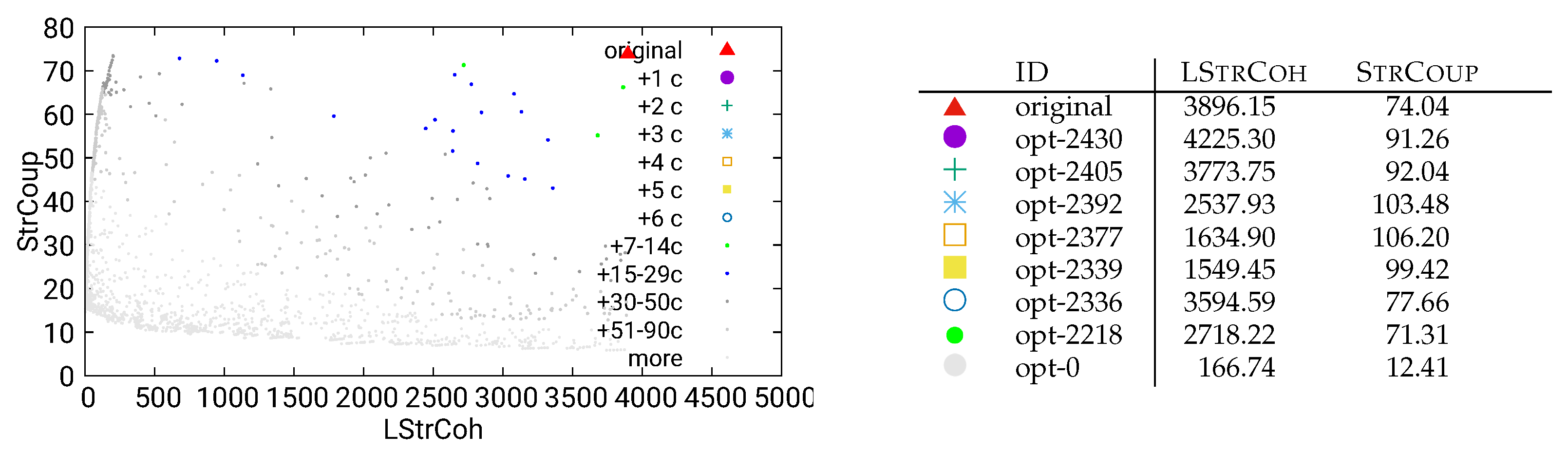
Figure 7.
Unguided optimization of MITgcm (global-ocean-cs32x15) using static/dataflow data
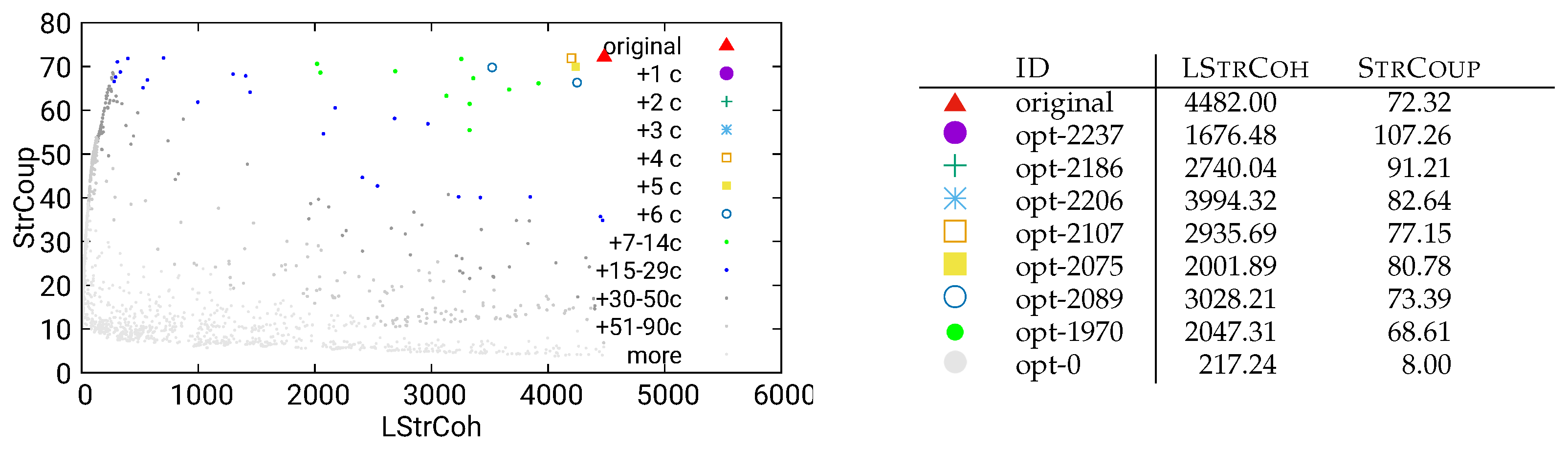
Figure 8.
Unguided optimization of MITgcm (global-ocean-cs32x15) using static/call data
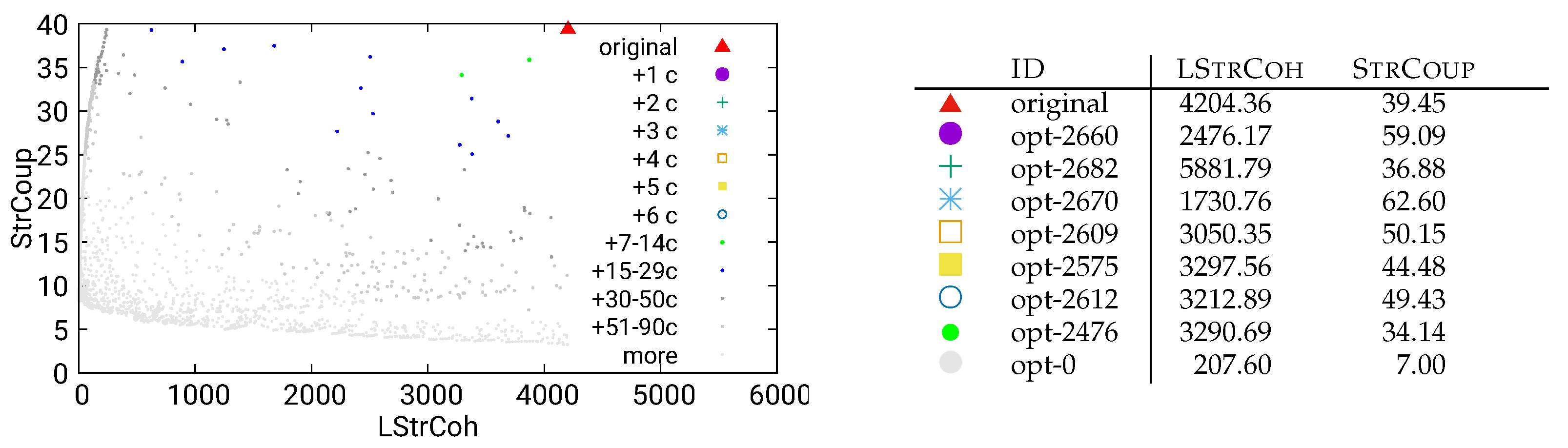
Figure 9.
Unguided optimization of MITgcm (global-ocean-cs32x15) using static/both data
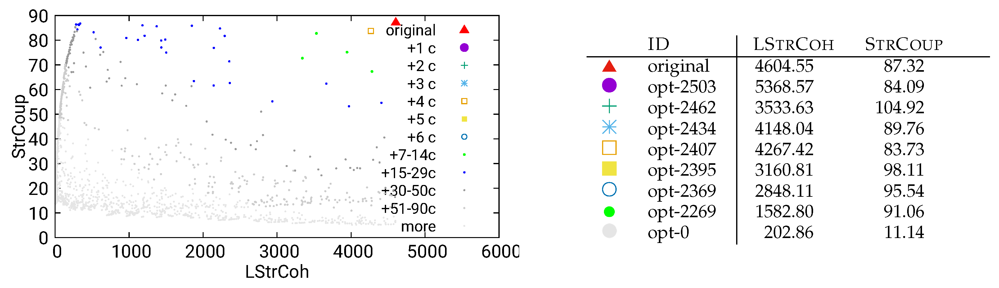
Figure 10.
Unguided optimization of MITgcm (global-ocean-cs32x15) using combined/call data
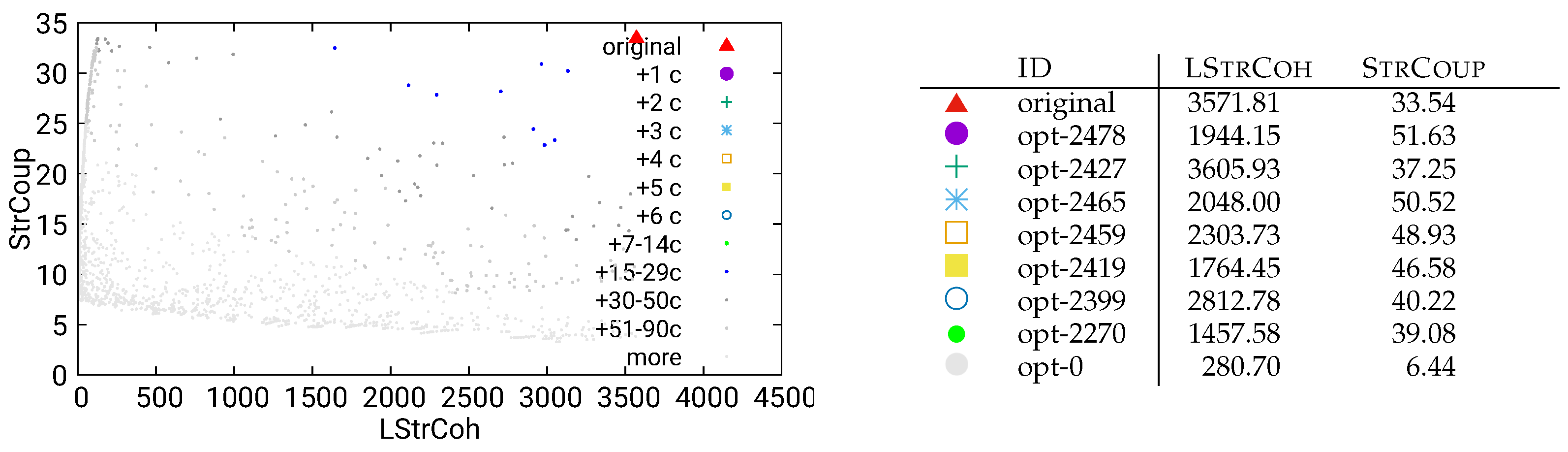
Figure 11.
Guided optimization of MITgcm (global-ocean-cs32x15) using dynamic/call data
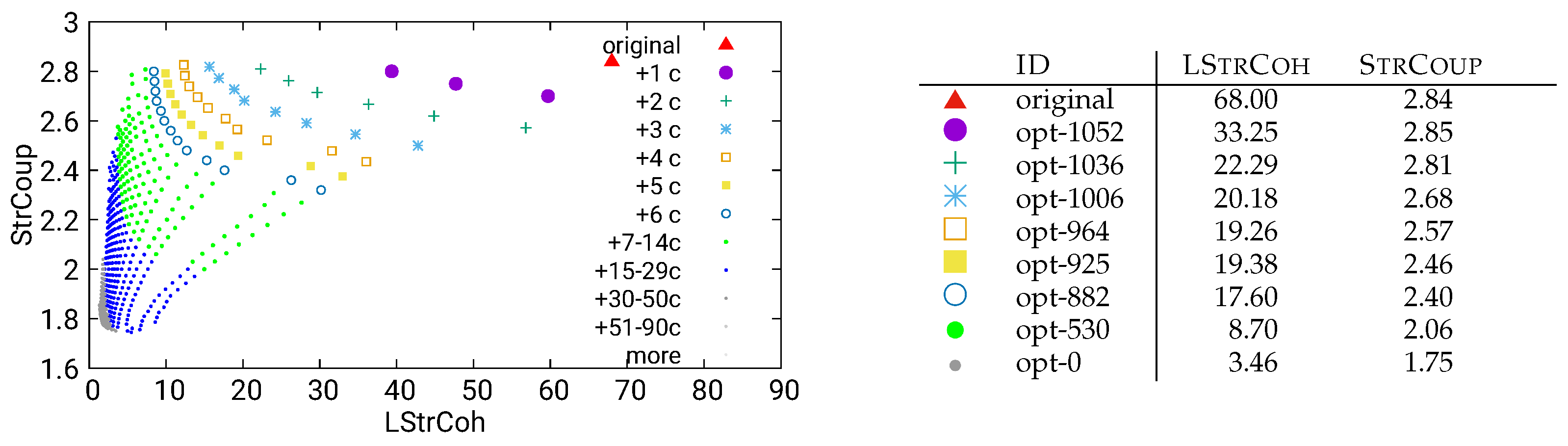
Figure 12.
Guided optimization of MITgcm (global-ocean-cs32x15) using combined/both data
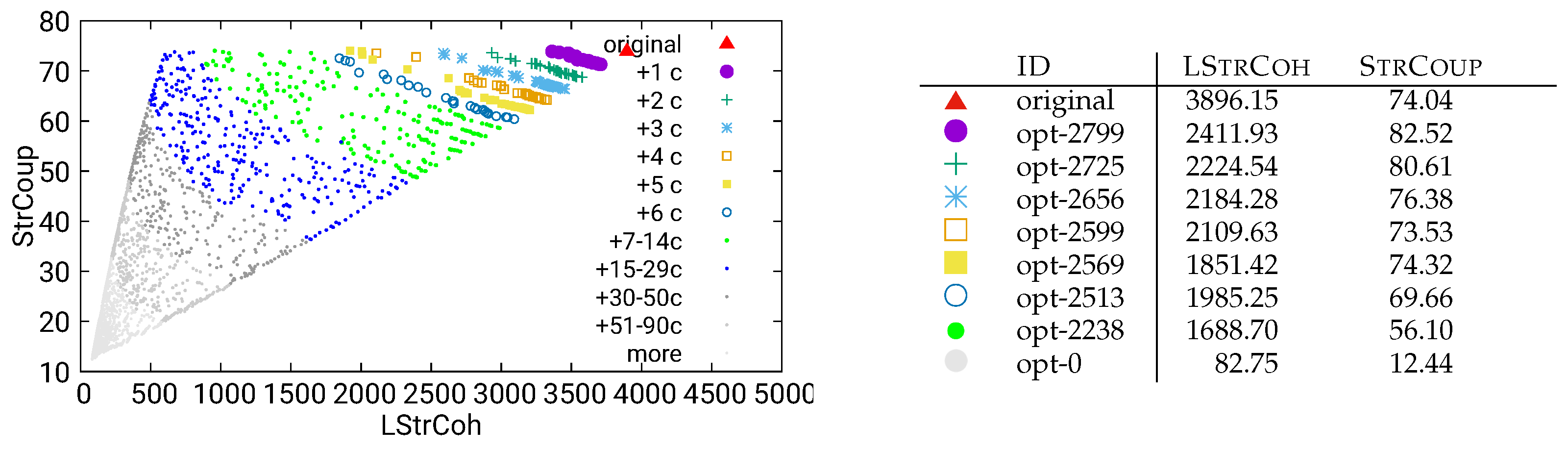
Figure 13.
Guided optimization of MITgcm (global-ocean-cs32x15) using combined/call data
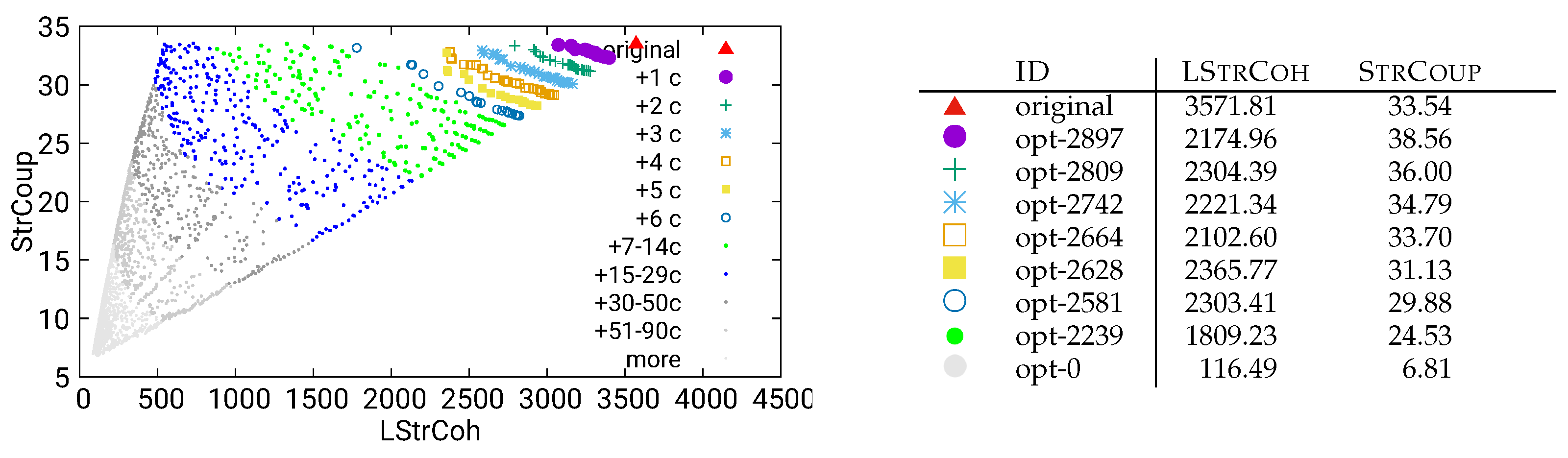
Figure 14.
Guided optimization of MITgcm (global-ocean-cs32x15) using static/both data
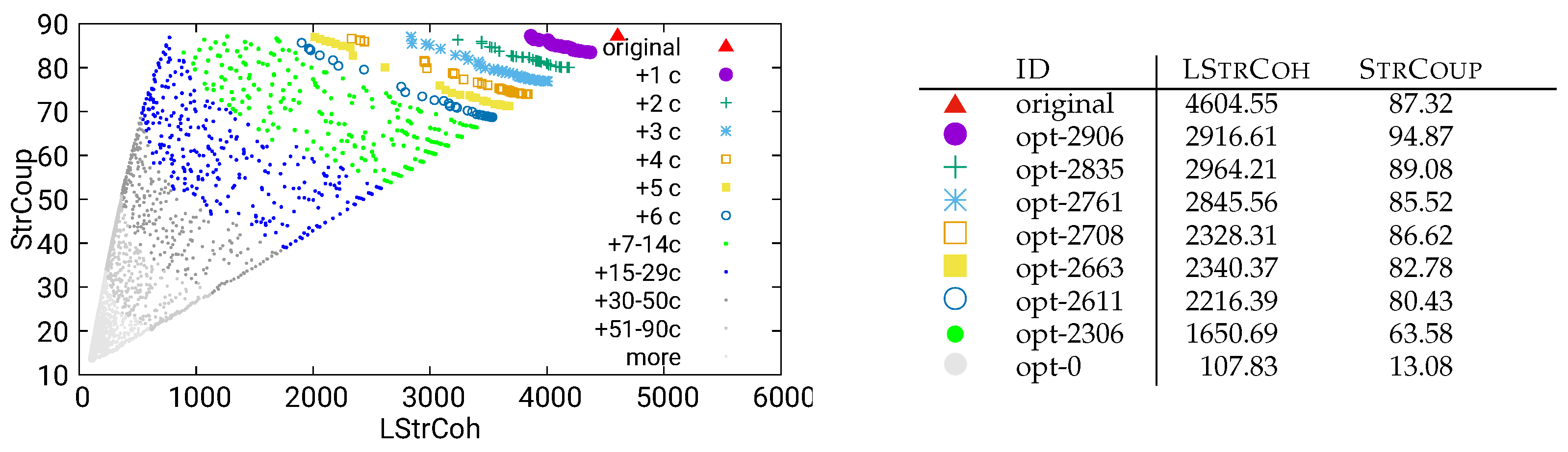
Figure 15.
Guided optimization of MITgcm (global-ocean-cs32x15) using static/call data
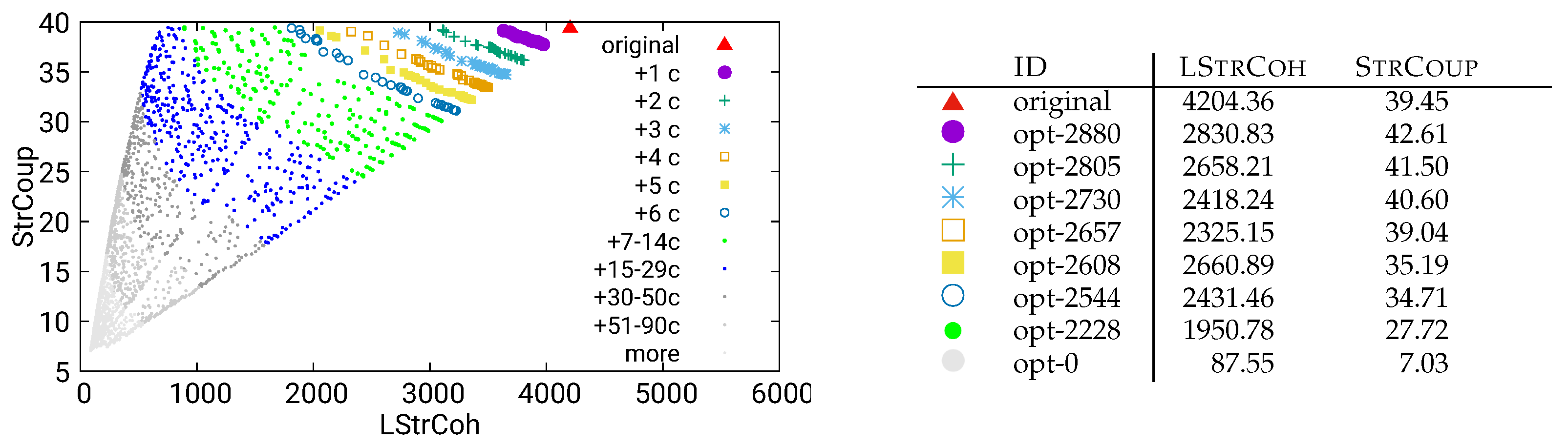
Figure 16.
Guided optimization of MITgcm (global-ocean-cs32x15) using static/dataflow data
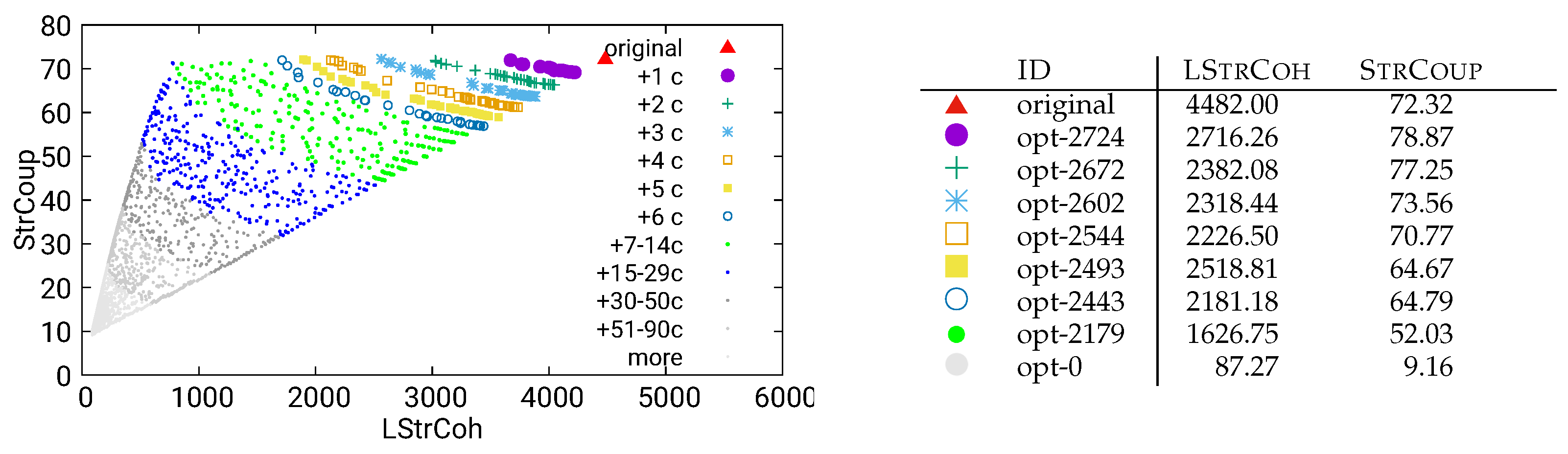
Figure 17.
Long running, unguided optimization of MITgcm using combined/both data
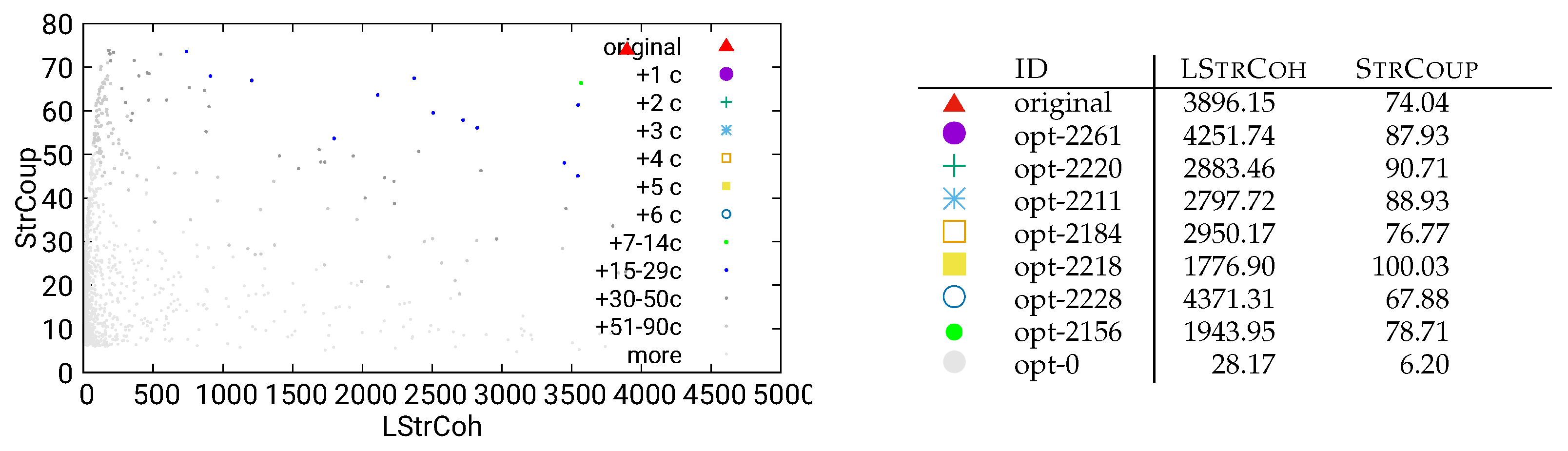
Figure 18.
Unguided optimization of UVic using dynamic/call data
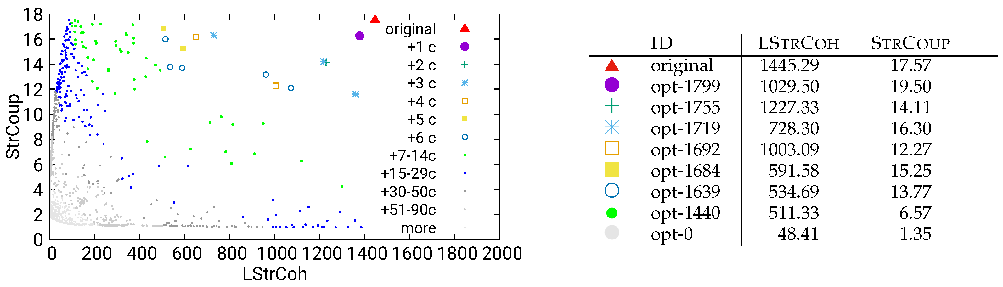
Figure 19.
Unguided optimization of UVic using combined/both data
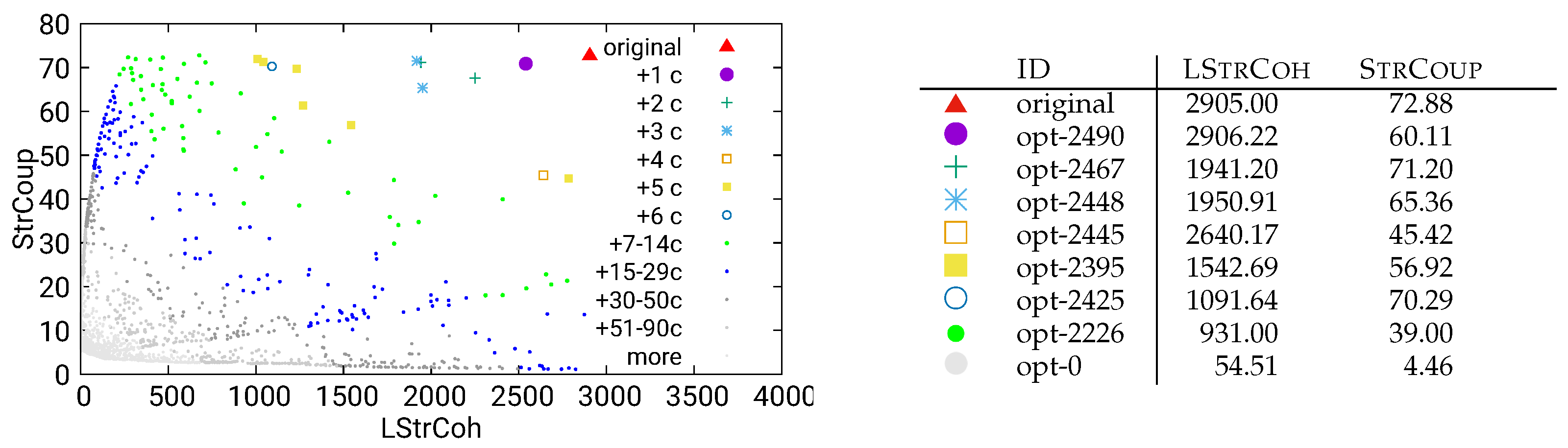
Figure 20.
Unguided optimization of UVic using static/both data
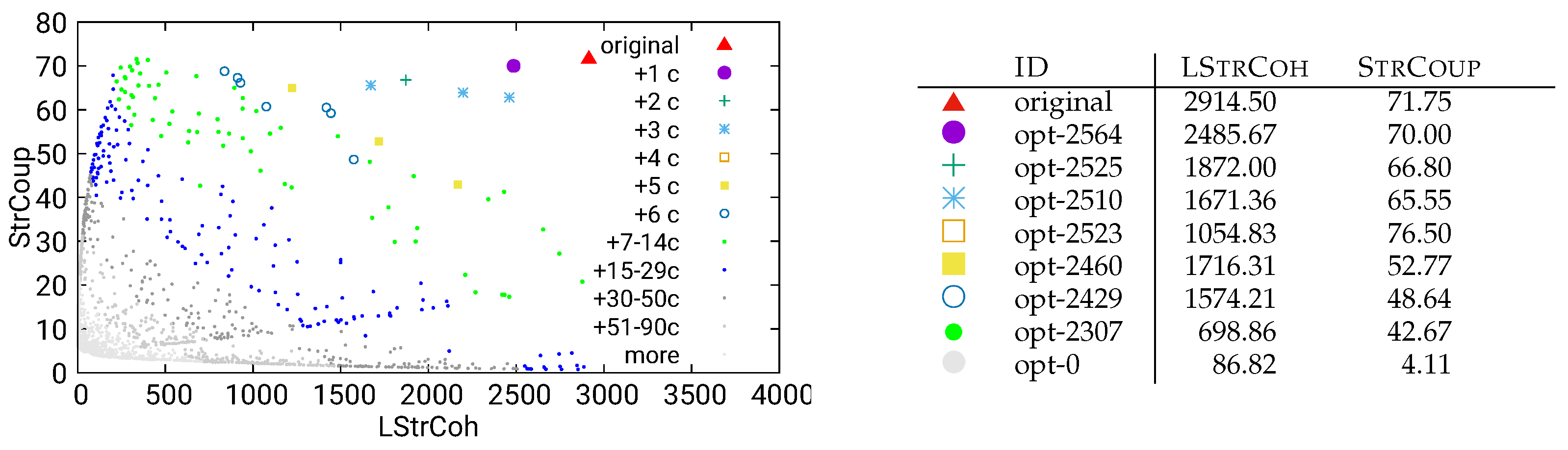
Figure 21.
Unguided optimization of UVic using combined/call data
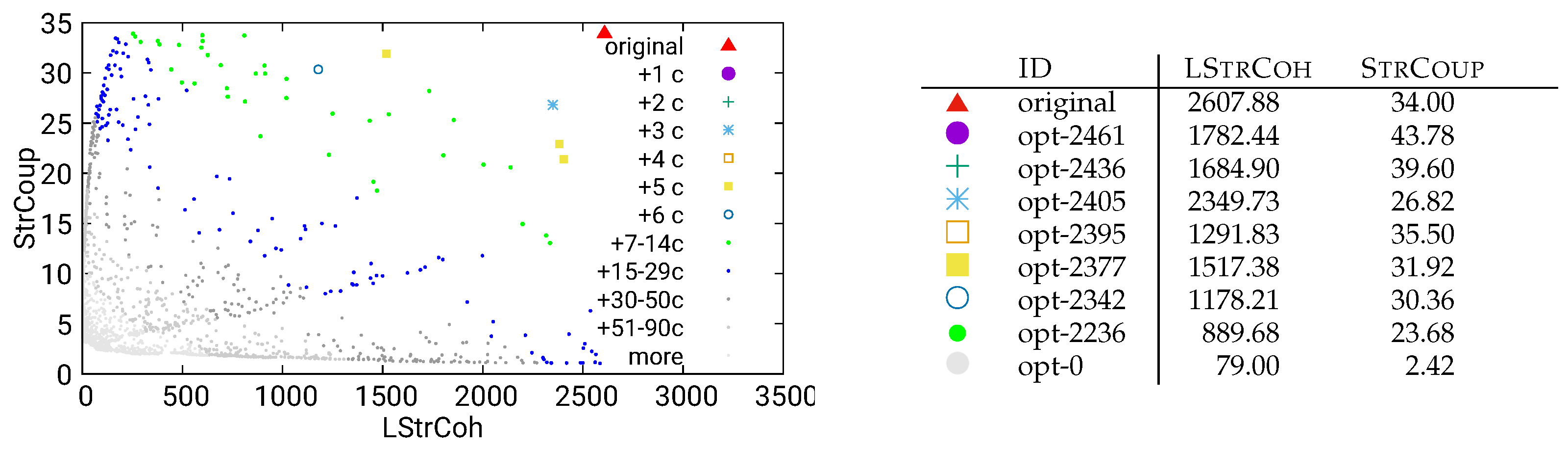
Figure 22.
Unguided optimization of UVic using static/call data
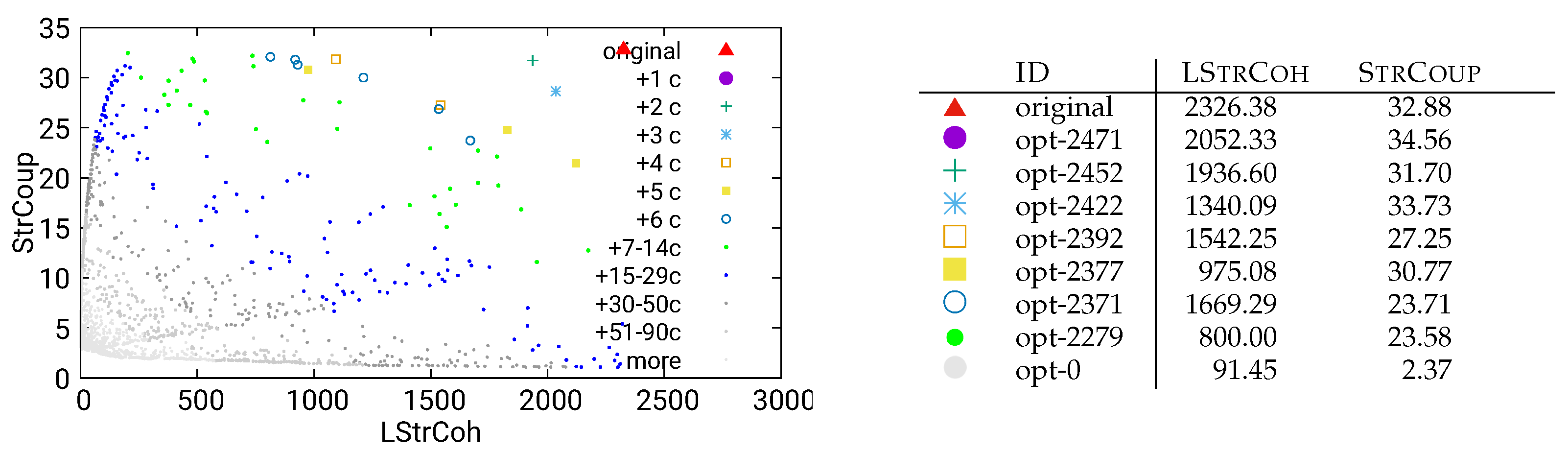
Figure 23.
Unguided optimization of UVic using static/dataflow data
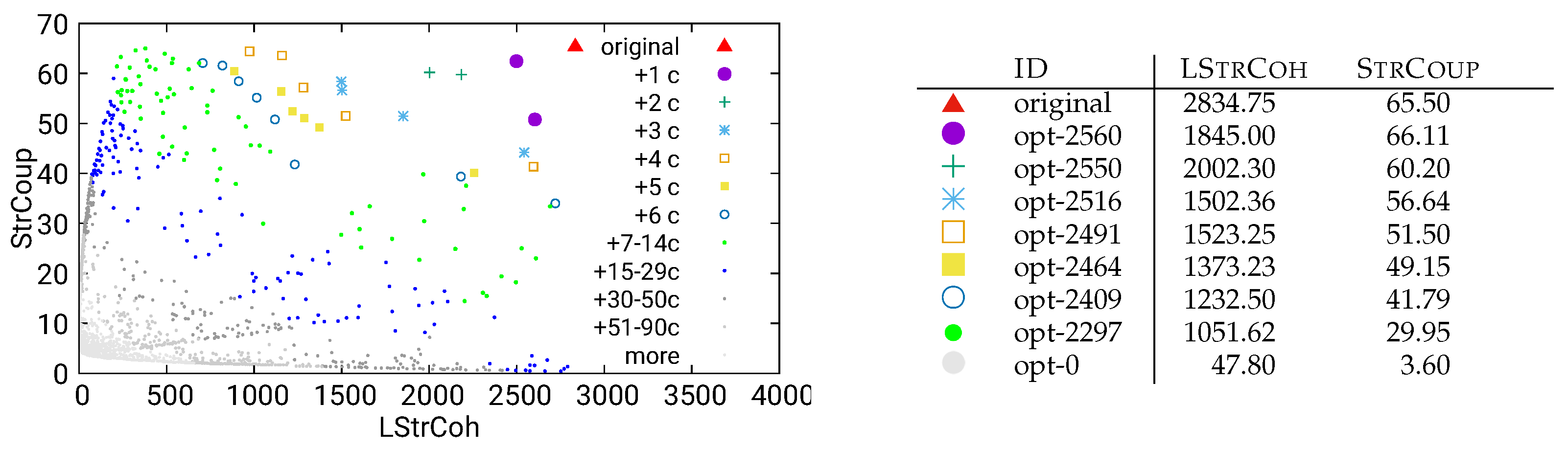
Figure 24.
Guided optimization of UVic using dynamic/call data
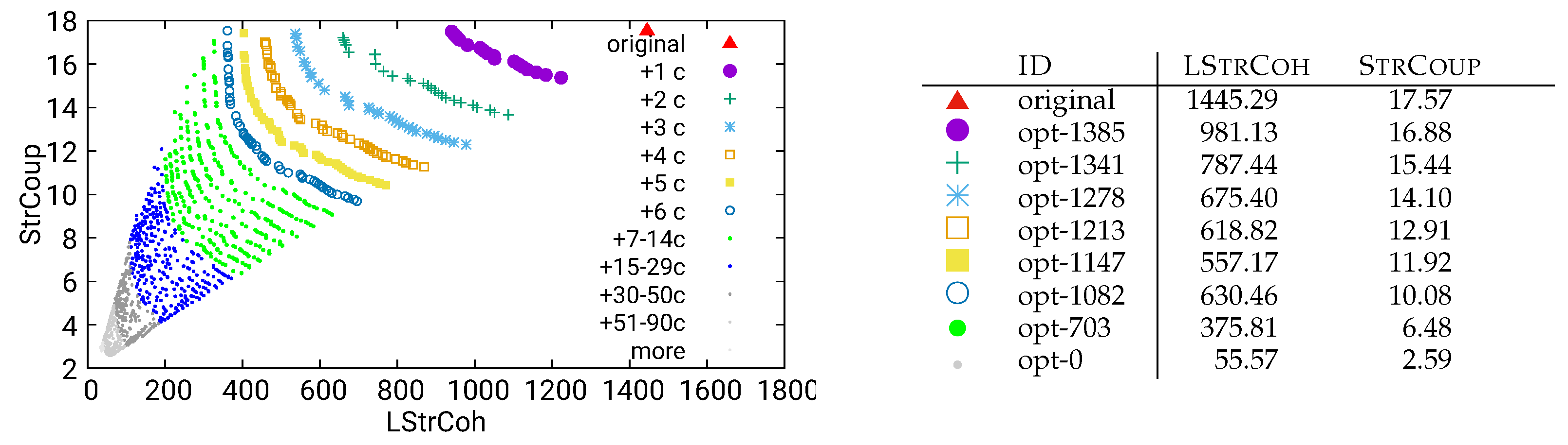
Figure 25.
Guided optimization of UVic using combined/both data
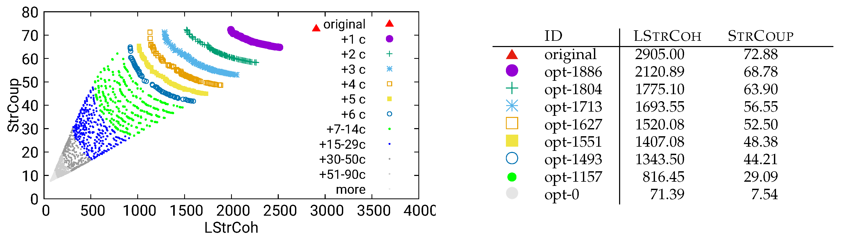
Figure 26.
Guided optimization of UVic using combined/call data
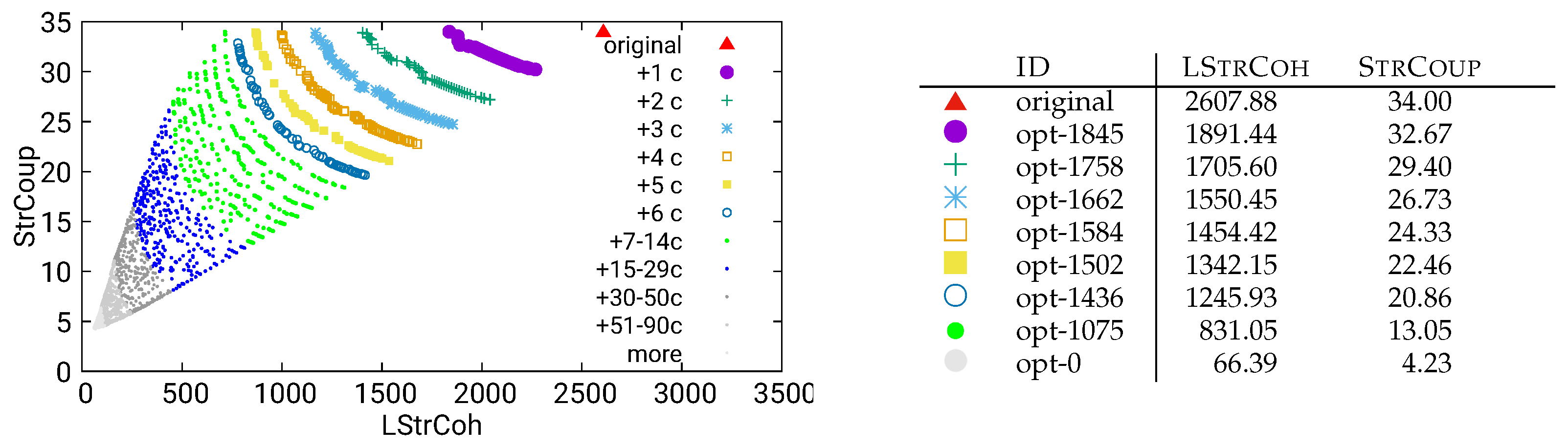
Figure 27.
Guided optimization of UVic using static/both data
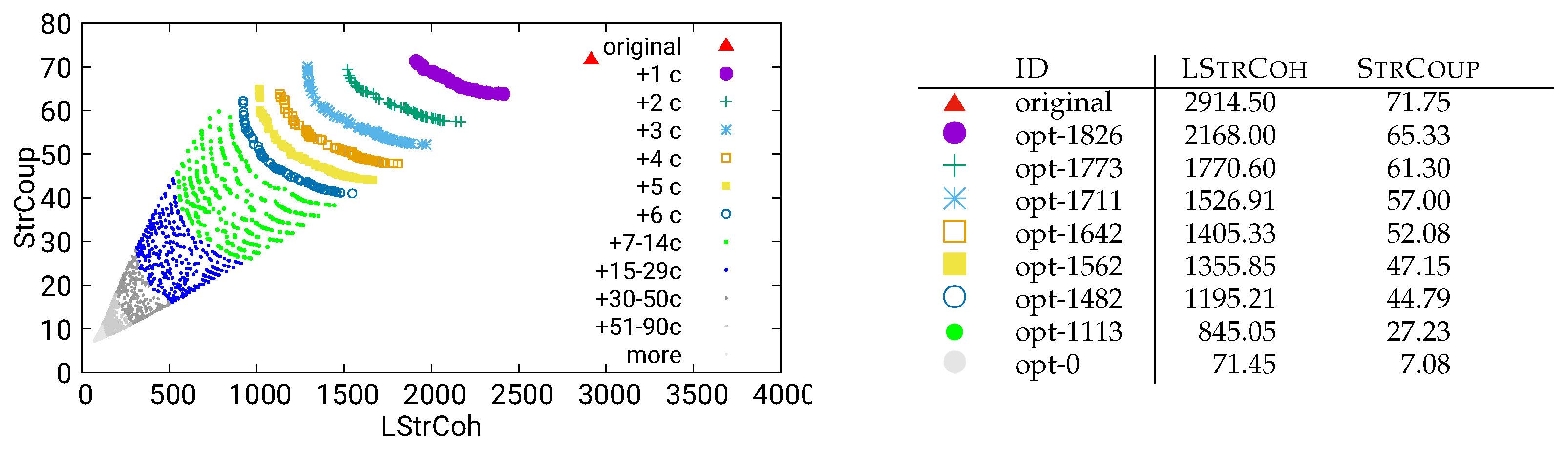
Figure 28.
Guided optimization of UVic using static/call data
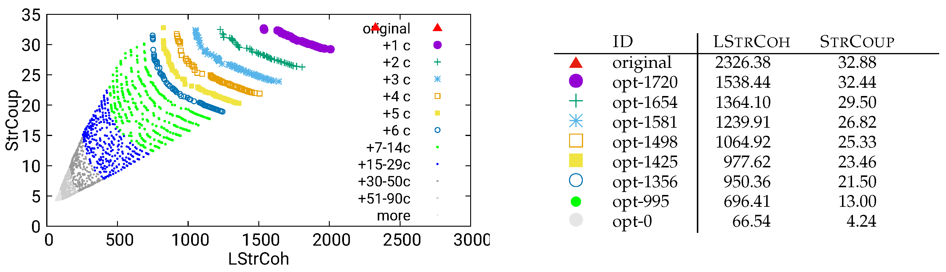
Figure 29.
Guided optimization of UVic using static/dataflow data
Disclaimer/Publisher’s Note: The statements, opinions and data contained in all publications are solely those of the individual author(s) and contributor(s) and not of MDPI and/or the editor(s). MDPI and/or the editor(s) disclaim responsibility for any injury to people or property resulting from any ideas, methods, instructions or products referred to in the content. |
© 2025 by the authors. Licensee MDPI, Basel, Switzerland. This article is an open access article distributed under the terms and conditions of the Creative Commons Attribution (CC BY) license (http://creativecommons.org/licenses/by/4.0/).
Copyright: This open access article is published under a Creative Commons CC BY 4.0 license, which permit the free download, distribution, and reuse, provided that the author and preprint are cited in any reuse.


