
Submitted:
04 August 2025
Posted:
05 August 2025
You are already at the latest version
Abstract
This paper presents a time-continuous Galerkin finite element method for the fully intrinsic geometrically exact beam equations that is energy consistent. Within the grid of space and time, this study derives the governing equations for elements using the Galerkin method and Time finite element method, implements variable-order interpolation of variables by Legendre functions, and establishes an assembly process for sapce-time finite element equations. Additionally, by introducing kinematical equations of the rotation with Lagrange operators completely impose the conservative loads into fully intrinsic equations. Through a set of illustrative examples, our algorithm demonstrates effectiveness in addressing conservative forces, static deformation, dynamic response which means the capabilities to analyze elastically coupled dynamic problems of helicopter rotor. Meanwhile, by increasing interpolation orders effectively enhances computational accuracy and reduces discrete grid requirements.
Keywords:
time-continuous Galerkin method
; fully intrinsic geometrically exact beam
; variable-order interpolation
; legendre functions
; conservative load
1. Introduction
Many engineering components can be idealized as beams that have one of their dimensions larger than the other two, e.g., helicopter rotor blades. In the field of aircraft design, beam structure is widely used as the main load-bearing structure of which dynamic problem has always been one of the important topics.
In recent years, the increasing complexity of rotor structure and analysis conditions has put forward higher requirements for blade dynamics models, among which the fully intrinsic geometrically exact beam theory [1] stands out with its unique form of first-order nonlinear partial differential equations that independent of displacement and rotation variables. Ghorashi [2] applied the general nonlinear intrinsic equations of the beam to solve the elastodynamic response of the hingeless composite blade under the condition of accelerating speed, and successfully analyzed the nonlinear response of the active airfoil blade and its influence on the steady-state load. Amoozgar [3] modeled the rotation dynamics of morphing composite blade by using full intrinsic geometrically exact beam equations, and solved them by finite element method. The convergence results were in good agreement with the experimental results. In [4], modeling methods of fully intrinsic geometrically exact beam under different boundary conditions are explored, and used for static equilibrium, steady-state motion, and linearized dynamic analyses. The results show the full intrinsic method is particularly suitable for blade dynamics analysis.
The derivation of full intrinsic form starts from the study of geometrically exact beams, which first appeared in the work of Kirchhoff and Clebsch [5] in 1944. Subsequently, according to different solving variables, the beam theories can be divided into three types: displacement-based scheme [6] that reduces the complexity of the formula by using high-order truncation, mixed variational scheme [7] that introduces generalized velocity and generalized strain as unknown variables, and fully intrinsic scheme [8] which completely eliminate displacement and rotation variables. The concept of intrinsic was first introduced by Green and Laws [9] in 1966 in the process of studying elastic rods. In 1977, Hegemier and Nair [10] proposed a fully intrinsic elastic rod theory with large deformation and small strain, that governing equations were composed of load and velocity variables, and were used to solve the steady-state motion of helicopter rotor blades. In 1990, Hodges [7] has developed an exact intrinsic formulation, which can be written in a simple matrix form with only second-degree nonlinearities and ideally suited for finite element method. The feasibility of finite element method solve mixed variables equation is verified in [11]. With the canonical form of the equations of motion, in 2003 Hodges [8] derived a set of generalized strain-velocity compatibility relations. Then make up a complete set of fully intrinsic and geometrically accurate partial differential equations of beam dynamics, which are energy conserved.
The fully intrinsic geometrically exact beam equation is a kind of nonlinear time-domain dependent partial differential equation, which is usually solved by a discrete process of first space then time, and the partial differential equations are transformed into time-domain recursive equations. Since the finite difference method is a simple and convenient spatial discreting method, Patil and Hodges [12] applied the fully intrinsic model to the dynamic analysis of highly flexible wing with the central difference scheme. This spatial discreting scheme was later used by Khouli [13] to analyze the hinged swept blade. In 2011, Patil and Althoff [14] used the continuous Galerkin method to discrete the fully intrinsic equation in space, and fitted the variables with Legendre polynomials. The results show that the Galerkin method can obtain more accurate solutions with fewer trial functions. In the same year, Patil and Hodges [15] proposed the concept of variable order finite element by changing the order of Legendre function, which compared the accuracy, computational efficiency and applicability to general problems. The results presented show that one can obtain approximately third-order, fifth-order, seventh-order, and ninth-order convergence for the linear, quadratic, cubic, and quartic finite elements. And one can use higher-order finite elements for a better approximation of mode shapes. In recent years, there have also been many spatial solving formats with better efficiency and accuracy, such as GDQ method [16] and neural network model [17]. However, these numerical algorithms always need to recurse gradually over time, often require a lot of time cost to iterate, have cumulative errors and greatly depend on the initial value.
The space-time finite element method is a high-precision and effective method to solve the problem of the development of time partial differential. Its main feature is to treat the time domain as the space domain for unified discretization, forming an unstructured grid in the sense of space and time, which is consistent for any order of discretization. Higher-order methods can be naturally embedded in these schemes, and have excellent characteristics of high calculation accuracy and moderate calculation amount in the field of nonlinear dynamics problems. Currently, there are relatively few time finite element methods for solving fully intrinsic geometrically exact beams. In [8], Hodges adopted the central difference scheme to discrete the space and time of equations simultaneously. Chen Lidao [18] adopted a DQ-Pade method with high order accuracy to construct the space-time finite element equation of the fully intrinsic model. In 2023, Chen Lidao [19] established a space-time finite element steady-state scheme based on Galerkin weighted residual method with Legendre functions, which has been successfully applied to non-conservative load issues. This discrete scheme is simple in structure and easy to assemble, but only the influence of linear and second-order schemes on the results was compared.
The present work is based on the general steady-state format derived in Ref. [19], The basic process of the Galerkin space-time continuous finite element method of the fully intrinsic geometrically exact beam is: Firstly, the space-time element control equation is obtained by discretization of the global elements along the spanwise and azimuth Angle of the blade. Then, assembling the element equations according to certain laws to get the total algebraic matrix equation of beam. Finally, solve it by Newton method and reverse displacement. Besides, the discontinuity treatment of blade structure, energy conservation of equation, initial value format, conservative load treatment and the influence of variable order are investigated. And a series of static deformation and dynamic response issues are given to verify the effectiveness of proposed algorithm.
2. Fully Intrinsic Beam Equations
Ignoring the warping deformation in the profile, the full intrinsic equations of the geometric exact beam theory can be expressed in a compact form as
Here, is the first partial derivative of space, and is the first partial derivative of time, is the initial twist/curvature of the beam, , and respectively represent the element distribution force and element distribution moment loaded on the beam that the direction is perpendicular to the beam axis. , , and are respectively representing the force, moment, linear velocity and angular velocity of the beam section at the location and time . , , and respectively representing the force strain, moment strain, linear momentum and angular momentum of the corresponding beam section. Note that all the intrinsic variables are expressed in the deformed base B as ( )B. is the cross product operator, taking as an example:
The constitutive equations relate the momenta to the velocities and the strain measures to the sectional loads as
Where, the matrix , and constitute the flexibility characteristics of the beam section, and the matrix , and respectively represent the linear density, mass eccentricity and moment of inertia. Equations (1) and (3) constitute a complete set of differential equations for first-order partial derivatives in time and space.
For a hingeless beam with length L, the spatial boundary and periodic continuity conditions of the steady-state problem can be summarized as follows:
Here, and represents the load condition at the free end, and are the velocity condition at the root of the blade. Let ( )0 represent the initial time state, thus the initial value boundary conditions of the transient problem can be similarly summarized as:
3. Galerkin Space-Time Finite Element Method
According to the work in [19], the fully intrinsic equations is naturally adapted to the Galerkin space-time continuous finite element method (STFEM). But only the analysis of low order scheme is given, lacking the comparison of high order algorithm. This paper will construct a variable-order scheme of the STFEM.
3.1. Conservation Laws of the Galerkin Space-Time Equations
For a hingeless rotor blade, consider the following weak form of all the equations (fully intrinsic equation, space boundary condition and time boundary condition), premultiply , , and by the Galerkin weighted method, and integrate in the spanwise and time domain:
Note that the constitutive equations are already satisfied exactly. With the rules of tilde notation , simplify the Eq. (6) as
Integrating by parts in space,
By the constitutive laws, integrating by parts in time,
Here, bring the kinetic energy and strain energy into evidence, which leads to:
The first term on the left side of the equation is the final energy, the second term is the initial kinetic energy, and the third term is the initial potential energy. The first term on the right of the equation is the work done by the distributed load, and the second term is the work done by the concentrated load at both ends of the beam. The equations states that the change of energy of the beam is equal to the work done on the beam. Thus, the above equations is an energy balance equations. The above convidence is valid in every space-time element. When dealing with periodic steady state problem, replace the time initial condition by periodic continuous condition, without breaking the conservation of equation.
3.2. Discretization in the Space-Time Domain
The integral domain of the above equation is then discretized as shown on the left in Figure 1. In the process of rotation, the blade with length L is dispersed into Ns segments along the spanwise. For any motion duration T which is multiple of the rotation period for the steady-state format, is dispersed into Nt segments along the azimuth Angle. Ultimately, form a global space-time cell grid on the scale of . The Eq. (6) must be satisfied in each element, and simultaneously convert the boundary conditions into continuity between adjacent elements.
Taking the element Eij, which is ith(i=1~Ns) in space and jth (j=1~Nt) in time, shown on the right in Figure 2. The spacial length of this element is denoted as Li, and the temporal length is denoted as Tj, while 0 represents the start position or the initial time. The variables within the element are denoted as Qij(x,t) that substitute for intrinsic variables among which (x,t) are coordinates in the element. The lines around the element are shared with the four elements around time (Ei,j-1, Ei,j+1) and space (Ei-1,j, Ei+1,j), that is, the continuous variables should be continuous with the adjacent elements or meet the boundary conditions. For a homogeneous blade, the continuity condition can be summarized as follows:
The above continuity conditions are applicable to any element with concentrated mass and initial deformation, thus the space-time finite element equation is as following:
Divide the above equation into four equations by the preceding multiplicative term:
The Eqs. (13), (14) are the dynamic equations of the element, and the Eqs. (15), (16) are the kinematic equations. When Eqs. (13)-(16) are both satisfied, Eq. (12) is established.
3.3. Separation of Variables in Space and Time
As for the dimensions of time and space are independent of each other, assume the intrinsic variables can be written as a linear combination of the products of a series of trial functions:
Here, is the column vector of distinct polynomial weights, and , . The independent trial functions used are the shifted Legendre function [20] that are orthogonal with the domain [0,1], and can well fit the boundary and periodic conditions. The polynomials can be iteratively derived as:
Therefore, the derivatives of variables can be expressed as the derivatives of spatial or temporal interpolation polynomials, respectively:
The continuity condition can be expressed as the continuity of the value of interpolating polynomial at ends (0 or 1) of the elements:
Let , , and respectively represent the weights of corresponding variables , , and . According to the Eqs. (3), (19), (20), transform the element fully intrinsic equations (13) - (16) into an algebraic system about the weight coefficients:
Here, a lot of subscripts (ab, kl, pq) are used to distinguish the order of polynomial. Especially, each group of subscripts corresponds to a different variable. And within each group, one is of temporal interpolation order between 0~Rs and the other is of spatial interpolation order between 0~Rt. Furthermore, during the processing of the premultiplication term, each equation is required to satisfy by any , , and , so it can be mentioned outside the equations.
3.4. Assemble Element Algebraic Equations
Take one weight coefficient out of the integral, and sort the integrals in Eqs. (21)~(24): the terms without variables in the integral are classified as linear matrices , the cross terms with variables in the integral are classified as nonlinear matrices , the terms without variables outside the integral are classified as constant matrices , and the variables outside the integral belong to adjacent elements , and are classified as continuity matrices that contain spatial continuity matrices and , and time continuity matrices . Thus, the element equation can be summarized in the following matrix form:
Here, is the column vector of dimension.
The system computing model of the structure is composed of all the space-time elements, and the structural characteristic matrix of the system is composed of superposition of each element coefficient matrix. On the basis of obtaining the above element matrix equation, then assemble the beam system equation according to the order of first space next time, as shown in Figure 2.
First of all, the equation variables are integrated: the jth time node variables are obtained by arranging the space-time element variables according to the spatial sequence of 1~Nt. Then the system unknowns are obtained by arranging different time node variables according to time sequence of 1~Ns.
Then, Assemble the coefficient matrix of each element according to the arrangement logic of variables:
- (1)
- Total stiffness matrix: The spatial continuity matrix , and the linear matrix are arranged side by side in the order of space formed as , then put it at row and colume to form the time node matrix . The element time continuity matrix is arranged on the diagonal in spatial order to form the time node continuity matrix . The time correlation matrix and are arranged in the order of time formed as , then put it at row and colume to form the total stiffness matrix.
- (2)
- Total nonlinear matrix : The element nonlinear matrix is arranged diagonally in space order formed as , and then diagonally in time order.
Finally, the constant matrix is assembled according to the assembly logic of the variables: first, the element constant matrix is placed in the row to form the time constant matrix , and then it is placed in the row to form the total constant matrix that includes external loads and boundary conditions.
So the assembled algebraic equations can be written as follows:
It should be noted that the time continuity matrix on the corner of the stiffness matrix in the initial value scheme is zero and the initial value condition will be contained in the constant matrix. When the number of elements is 1, the whole domain is taken as a element, eliminating the process of discretization and assembly, but the variables in the domain are required to be consistent, that is, the profile characteristics are continuous, and in the periodic scheme, the matrix is implicit in the matrix .
Newton-Raphson method is used to solve the nonlinear system equations with the Jacobian matrix that can be expressed accurately. Here's a simple demonstration, supposing the Eq. (26) is
Then the Jacobian matrix is
The iterative initial value is taken by dividing the blade stiffness matrix with the constant matrix, i.e . According to the result of each step, the Jacobian matrix is updated and the variables are iterated until convergence. The result is substituted back to Eq. (17) to get the space and time distribution function of the intrinsic variables.
After obtaining the global distribution of the intrinsic variables and rotation matrix, it is still difficult to imagine the displacement and rotation angle of the beam, so it is necessary to convert the results to the configuration space. For this purpose, the displacement can be reversed by the following displacement-strain equation and displacement-velocity equation:
Here, is the displacement in the undeformed coordinate system and is the linear velocity of the undeformed blade. Similarly, the theta of rotation can be reversed by rotation kinematical equations which is:
Here, is the angular velocity of the undeformed blade, and is a 3x3-dimensional tensor matrix, which represents the rotation of the section from the undeformed coordinate to the deformed coordinate with . The initial value conditions of displacement and rotation are:
To represent the angle in the undeformed coordinate system, according to the specific expression of the coordinate transformation matrix which is no singularity, it is obtained:
3.5. Flow of Space-Time Finite Element Method
The basic flow of space-time finite element method (STFEM) for fully intrinsic geometrically exact beam equations can be summarized as follows:
- Galerkin space-time equation for a hingless blade is Eq. (6). Discrete the space along the beam, and discrete the time along the azimuth angle in each movement period, then obtain the global discrete space-time grid as Figure 1;
- Establish the continuous relationships between units as Eqs. (11). Thus the space-time finite element equation can be obtained by the weighted method as Eq. (12), divide it into four equations according to the different weight functions like Eqs. (13) - (16).
- With the Legendre functions Eq. (18), approximate the variables to a linear combination of a set of spatio-temporal polynomials as Eq. (19). Then variables are only the weight coefficients of polynomials and transform the derivative terms and continuity into the derivative and continuity of polynomials as Eq. (20). Thus the finite element algebraic equations are obtained as Eqs. (21)~(24).
- Take one weight coefficient out of integral, classify the integral functions according to the number of variables, then the matrix equation Eq. (25) of element is obtained.
- Assemble the above element matrix equation according to a certain law as show in Figure 2. Then the global discrete algebraic equation Eq. (26) of beam are obtained whose coefficient matrix only includes stiffness matrix, nonlinear matrix and constant matrix;
- Gain the linear initial value as and the Jacobian matrix like Eqs. (27), (28). The Newton method is used to solve the nonlinear equation, and the global distribution of the intrinsic values is sorted out.
- Given the initial conditions of displacement and rotation angle like Eq. (31), obtain the displacement distribution in the entire domain by Eq. (29) and the transformation matrix distribution by Eq. (30), then get the theta distribution by Eq. (32).
3.6. Treatment of Blade Structure Discontinuity
It should be noted that in the actual design process, there is a discontinuity in the blade structure, that is, the section structural characteristics are discontinuous which lead to a discontinuity of load. According to the constitutive law, the fact that the strain is continuous in the spatial direction does not mean that the load is uniformly continuous:
Where, and represents the left and right parameters of the discontinuous section, [S] is the profile stiffness matrix. Therefore, the spatial continuity of the load at the discontinuity section can be established by the section flexibility matrix [R] as:
When the left and right characteristics of the section are consistent, Eq. (32) naturally degenerates into Eq. (3).
3.7. Handling of Conservative Loads
In the process of rotor movement, the main external force is the aerodynamic load following the deformation, which completely fits to the coordinate system of the fully intrinsic model. In addition, the blade is also affected by gravity, although the value is small compared with the aerodynamic force, but in many cases can’t be ignored.
Refer to Ref. [21], a coupling scheme of geometrically exact equations combined kinematical equation was proposed by Lagrange multipliers. So that all the variables can vary independently in the calculus. This paper introduces the conservative loads through the coupling of rotation kinematical equations. Thus, by coupling Eq. (30) with Eq. (1) through Lagrange multipliers, it can be obtained:
Here, and are the conservative force and moment. The Lagrange multipliers always can be identified by conservation of energy and it is a three-dimensional column vector that can be deal with Eq. (17). Since can be independently and arbitrarily varied, its specific form does not affect the process of the method proposed in this paper. Similarly, make modifications to the load boundary conditions with conservative tip force and tip moment :
4. Numerical Results
In order to verify the effectiveness of the algorithm presented in this paper, the influence of higher order scheme and the ability to solve large deformation problem under conservative load, four cases are presented. Firstly, investigated by applying the concentrated tip moment with different order or elements. Secondly, non-conservative tip force and conservative tip force are applied on the cantilever beam. Thirdly, Minguet beam experiment were conducted to verify the ability under conservative load with common structural coupling. Finally, the dynamic response problem of rotating or non-rotating beam proves the validity of the initial value scheme.
4.1. Large Deformation Simulation of Bending Moment on Elastic Beam Tip
The first case is a benchmark problem for the geometrically nonlinear analysis of beams [22]. A flapping moment is applied to the tip of an elastic beam clamped at root. The parameter of the beam is , . Each point on the beam will be located on the arc with curvature , and its exact solution can be expressed as:
Under the tip bending moment, only the bending moment exists at each point of the fixed beam, and the value is equal to the tip bending moment. This means the variables are only constants that the Legendre interpolation order is not sensitive to this problem and is only relevant to the algorithm error. The displacement is obtained by solving the approximate solution of the differential equation, whose error is closely related to the deformation degree and mesh density.
Table 1 list the tip position r3 under different tip bending moments with single one element, and Table 2 list the tip position r3 under different number of elements with a tip bending moments of 2500lb-ft2. All spatial elements adopt 9th-order interpolation. Through comparison, it is obvious that with the increase of deformation degree, the precision decreases obviously, and increasing the number of mesh can also improve the accuracy of the result. In Ref. [23], use the 20-element RCAS model, the magnitude of error is 6.00×10⁻⁴ when the tip bending moment is 500lb-ft2, which is far less than the calculation accuracy of a single element. While the magnitude of error is 1.98×10⁻⁴ when the tip bending moment is 2500lb-ft2, which can be achieved with only 3 elements.
Table 2 compares the differences between the interpolation functions order with the same number of elements. We can observe that as the element number increases, the two schemes tend to unify the solution, but when the number of units is less than 10 units, the error of the higher order scheme is significantly smaller.
4.2. Static Deflections of Cantilever with Conservative or Non-Conservative Load
Case 2 is the static deformation problem of a fixed beam under dynamic force [24,25]. The dynamic load is divided into two cases: the non-conservative and conservative force at the free end of the blade. The so-called non-conservative force is the direction of the force always perpendicular to the beam axis, while conservative force keeps in the original directions. The basic parameters of the beam are: length L=100cm, moment of inertia I22=1.666667cm4, material Young's modulus E=2.1x10⁷N/cm2.
The displacement-force curve of the free end of the beam under different non-conservative tip forces is shown in Figure 3, in which an obvious nonlinear large deformation of the beam can be seen. The simulation results of 5th-order 1-unit, 5th-order 2-units and 9th-order 1-unit are compared with the calculated data in Ref. 24 which is obtained by 10 elements and 30unknows. It can be noted that both the 5th-order 2-elements and the 9th-order 1-element are basically consistent with the reference results, except that the 5th-order 1 element deviates far under large deformation.
At the tip load of about 30kN, u1 deviates from the reference. According to the trend analysis, at this time, the beam is developing from linear to nonlinear deformation, the tip is gradually moving upward, the angle growth trend is gradually slowing down. So the tip should still be extending negatively, that is, the tip has passed the origin along the X-axis, and -u1/L is greater than 1. In addition, comparing the 5th-order 2-element and 9th-order 1-element, it can be found that when the beam is under large deformation, increasing the number of elements is closer to the result than increasing the order. This is because the displacement nonlinearity is more prominent than the load nonlinearity, and the mesh encryption can be more effective in fitting.
The displacement-force curve of the free end of the beam under different conservative tip loads is shown in Figure 4. It can be seen from the figure that both the 9th-order 1-unit and the 5th-order 2-unit are basically consistent with the reference results. Although there is a certain gap between the u3 of the 5th-order 1-unit and the compared data, the time error is not obvious when PL2/EI<6.
4.3. Static Behavior of Composite Blades Under Large Deflections
Composite materials have emerged as a primary material for helicopter rotor blades that leads to the presence of structural couplings such as extension-twisting and bending-twisting. These couplings can be used to improve the dynamic and aero-elastic performance of helicopter rotors. Case 3 is the large deformation problem of composite blade under static load [26,27], and examines the performance of the proposed algorithm for structurally coupled composite blade under large load conditions.
During the experiment, an aluminum chuck was used to fix the composite beam on the rotating platform to control the installation angle. The blade exposed outside the chuck was 550mm length and 30mm width. The strain gauge was attached at 50mm outside the chuck, and the displacement was observed at 300mm and 500mm. When the installation angle is 0°, the blade is placed horizontally. The STFEM with the 9-order 1-element format is used, compared with the finite difference method (FDM) in Ref. [28,29] which discretizes length into 56 nodes. In the experiments, the beam's own weight is included and all displacements are measured from initial position.
The first specimen has a [0/90]3s layup, without any coupling to serve as a reference, as shown in Figure 5. Among them, the displacement w is almost linear, and the displacement u is negative in practice. When the installation Angle is 0°, the displacement v is 0, and the tip deformation is about 40% of its length under maximum load. When the installation angle is turned to 45°, due to the weak rigidity in the normal plane, the deformation tends to be the initial v and w are basically the same. The calculation results of the method in this paper are basically consistent with those in the literature, which accords with the nature law and proves the reliability of the algorithm in the case of no coupling.
The next one is a [45/0]3s, to illustrate the effect of bending-twisting coupling, as shown in Figure 6. Due to the existence of flexural and torsional coupling, even at 0° installation Angle, there is a certain coupling deformation v, and it appears as v at 45°, and w is basically the same, but it is completely different at -45°. In general, although the algorithm in this paper has some shortcomings in u calculation, it is more close to the coupling change of v and w.
Meanwhile, a [20/-70/ -70/20]2a layup was used to illustrate the effect of extension-twist, as shown in Figure 7. Compared with uncoupled layup, the torsional stiffness was significantly enhanced. The results show that although there is a certain gap between the proposed algorithm and the experimental data, it is completely consistent with the results of the FDM.
4.4. Dynamic Response of Cantilever Beam
Two cases for dynamic response [30] are performed for hingeless boundary conditions with nonrotating or rotating to simulate in time domain of helicopter blades. The first one is a nonrotating beam with a tip dynamic forces along vertical orientation F3=10sin(20t). And the second one is a rotating beam under a tip force along transversal orientation F2=10sin(20t) with the rotating speed is 70 rad/s. The material properties of this beam are shown in Table 3.
Figure 8, Figure 9, Figure 10 and Figure 11 shows the time history curve of tip displacement, tip rotation, root force and root bending moment of a non-rotating cantilever beam under a given dynamic load F3=10sin(20t). The algorithm in this paper (STFEM) adopts a 5x5 cell, 5x5 order space-time format, and computes in a step of 0.3s. The calculation takes 4 steps, totaling 1.2s. Results Compared with the Dymore program, the waveform is basically the same, though there is a certain time delay with the development. On the whole, the calculated results in this paper are completely consistent with Ansys, which proves the accuracy and reliability of the proposed method.
Figure 12, Figure 13, Figure 14 and Figure 15 show the time history curve of tip displacement, tip rotation and root bending moment of a rotating clamped beam under a given tip dynamic load F2=10sin(20t). The format used is the same as above, the time step is 0.045s, and the total of 8 steps is 0.36s. According to the results, each peak and valley position can be clearly captured. Although the deviation in the pendulum torque is slightly large compared with other terms, the whole is consistent with the simulation code Dymore, which verifies the feasibility of the proposed algorithm in the aerodynamic analysis of blades.
5. Conclusions
In this paper, a space-time continuous finite element method for solving the fully intrinsic equations of geometrically exact beam is established successfully. The process of the space-time discretization, establishment of element equation, discretization of variables, assembly of equations and solution are described in detail. This space-time finite element scheme is energy conservation and variable order that has the potential of adaptive algorithm. This paper also provides solutions to common discontinuity problem, conservative load problem and initial value problem. The results show that this algorithm has good precision, stable convergence and ability to analyze the problem of blade coupling. By increasing the interpolation order of variables, the calculation accuracy is improved effectively, and the minimum number requirement of elements is significantly reduced that can even be developed into a meshless algorithm. In the following studies, the proposed method can naturally introduce aerodynamic equations to achieve aero-elastic adjoint solution, or as a high-precision dynamics solver, use loose coupling method to analyze the aero-elastic response of the rotor.
References
- Hodges, D.H. Nonlinear Composite Beam Theory; AIAA: Reston, VA, USA, 2006. [Google Scholar]
- Ghorashi, M.; Nitzsche, F. Nonlinear dynamic response of an accelerating composite rotor blade using perturbations. Journal of Mechanics of Materials and Structures 2009, 4, 693–718. [Google Scholar] [CrossRef]
- Amoozgar, M.R.; et al. Composite Blade Twist Modification by Using a Moving Mass and Stiffness Tailoring. AIAA Journal 2019, 57, 4218–4225. [Google Scholar] [CrossRef]
- Sotoudeh, Z.; Hodges, D.H. Modeling Beams with Various Boundary Conditions Using Fully Intrinsic Equations. Journal of Applied Mechanics 2011, 78, 31010-1–31010-9. [Google Scholar] [CrossRef]
- Love, A.E.H. Mathematical Theory of Elasticity, 4th ed.; Dover Publications: New York, New York, 1944. [Google Scholar]
- Bauchau, O.A.; Kang, N.K. A Multibody Formulation for Helicopter Structural Dynamic Analysis. J. Am. Helicop. Soc. 1993, 38, 3–14. [Google Scholar] [CrossRef]
- Hodges, D.H. A Mixed Variational Formulation Based on Exact Intrinsic Equations for Dynamics of Moving Beams. Int. J. Solids Struct. 1990, 26, 1253–1273. [Google Scholar] [CrossRef]
- Hodges, D.H. Geometrically Exact, Intrinsic Theory for Dynamics of Curved and Twisted Anisotropic Beams. AIAA J. 2003, 41, 1131–1137. [Google Scholar] [CrossRef]
- Green, A.E.; Laws, N. A General Theory of Rods. Proceed. Royal Soc. London 1966, 293, 145–155. [Google Scholar]
- Hegemier, G.A.; Nair, S. A Nonlinear Dynamical Theory for Heterogeneous, Anisotropic, Elasticrods. AIAA J. 1977, 15, 8–15. [Google Scholar] [CrossRef]
- Hodges, D.H.; Shang, X.; Carlos, C. Finite Element Solution of Nonlinear Intrinsic Equations for Curved Composite Beams. J. Am. Helicop. Soc. 1996, 41, 313–321. [Google Scholar] [CrossRef]
- Patil, M.J.; Hodges, D.H. Flight Dynamics of Highly Flexible Flying Wings. J. Aircr. 2006, 43, 1790–1798. [Google Scholar] [CrossRef]
- Khouli, F.; Afagh, F.F.; Langlois, R.G. Application of the First Order Generalized-α Method to the Solution of an Intrinsic Geometrically Exact Model of Rotor Blade Systems. Journal of Computational and Nonlinear Dynamics 2009, 4, 1–12. [Google Scholar] [CrossRef]
- Patil, M.J.; Althoff, M. Energy-consistent, Galerkin approach for the nonlinear dynamics of beams using intrinsic equations. J. Vib. Control 2011, 17, 1748–1758. [Google Scholar] [CrossRef]
- Patil, M.J.; Hodges, D.H. Variable-order finite elements for nonlinear, fully intrinsic beam equations. J. Mech. Mater. Struct. 2011, 6, 479–493. [Google Scholar] [CrossRef]
- Amoozgar, M.R.; Shahverdi, H. Analysis of Nonlinear Fully Intrinsic Equations of Geometrically Exact Beams Using Generalized Differential Quadrature Method. Acta Mechanica 2016, 227, 1265–1277. [Google Scholar] [CrossRef]
- Zhang, Z.; et al. A varying-gain recurrent neural-network with super exponential convergence rate for solving nonlinear time-varying systems. Neurocomputing (Amsterdam) 2019, 351, 10–18. [Google Scholar] [CrossRef]
- Chen, L.; Liu, Y. ; Differential Quadrature Method for Fully Intrinsic Equations of Geometrically Exact Beams. Aerospace 2022, 9, 596. [Google Scholar] [CrossRef]
- Chen, L.; Hu, X.; and Liu, Y. Space-Time Finite Element Method for Fully Intrinsic Equations of Geometrically Exact Beam. Aerospace 2023, 10, 92. [Google Scholar] [CrossRef]
- Abramowitz, M.; Irene, A.S. (Eds.) Handbook of mathematical functions with formulas, graphs, and mathematical tables. 55. US Government printing office. 1948. [Google Scholar]
- Wang, Q.; Yu, W. Geometrically nonlinear analysis of composite beams using Wiener-Milenković parameters. Journal of Renewable and Sustainable Energy 2017, 9. [Google Scholar] [CrossRef]
- Hopkins, A.S.; Ormiston, R.A. An Examination of Selected Problems in Rotor Blade Structural Mechanics and Dynamics. Journal of the American Helicopter Society 2006, 51, 104–119. [Google Scholar] [CrossRef]
- Hodges, D.H.; et al. Free-Vibration Analysis of Composite Beams. Journal of the American Helicopter Society 1991, 36, 36–47. [Google Scholar] [CrossRef]
- Argyris, J.H.; Symeonidis, S. Nonlinear finite element analysis of elastic systems under nonconservative loading-natural formulation. part I. Quasistatic problems. Computer Methods in Applied Mechanics and Engineering 1981, 26, 75–123. [Google Scholar] [CrossRef]
- Kondoh, K.; Atluri, S.N. Large-deformation, elasto-plastic analysis of frames under nonconservative loading, using explicitly derived tangent stiffnesses based on assumed stresses. Computational Mechanics 1987, 2, 1–25. [Google Scholar] [CrossRef]
- Minguet, P.J. Static and dynamic behavior of composite helicopter rotor blades under large deflections[D]. Massachusetts Institute of Technology, 1989. [Google Scholar]
- Minguet, P.J.; Dugundji, J. Experiments and analysis for composite blades under large deflections Part I: Static behavior. AIAA Journal 1990, 28, 1573–1579. [Google Scholar] [CrossRef]
- Dowell, E.H.; Traybar, J.J. An experimental study of the nonlinear stiffness of a rotor blade undergoing flap, lag and twist deformations[R]. 1975. [Google Scholar]
- Dowell, E.H.; Traybar, J.J.; Hodges, D.H. An experimental-theoretical correlation study of non-linear bending and torsion deformations of a cantilever beam. Journal of Sound and Vibration 1977, 50, 533–544. [Google Scholar] [CrossRef]
- Cheng, T. Structural dynamics modeling of helicopter blades for computational aeroelasticity. Doctoral dissertation, Massachusetts Institute of Technology, Cambridge, MA, USA, 2002. [Google Scholar]
Figure 1.
Schema of the space-time finite element discrete grid.

Figure 2.
Schematic diagram of element equation assembly process.
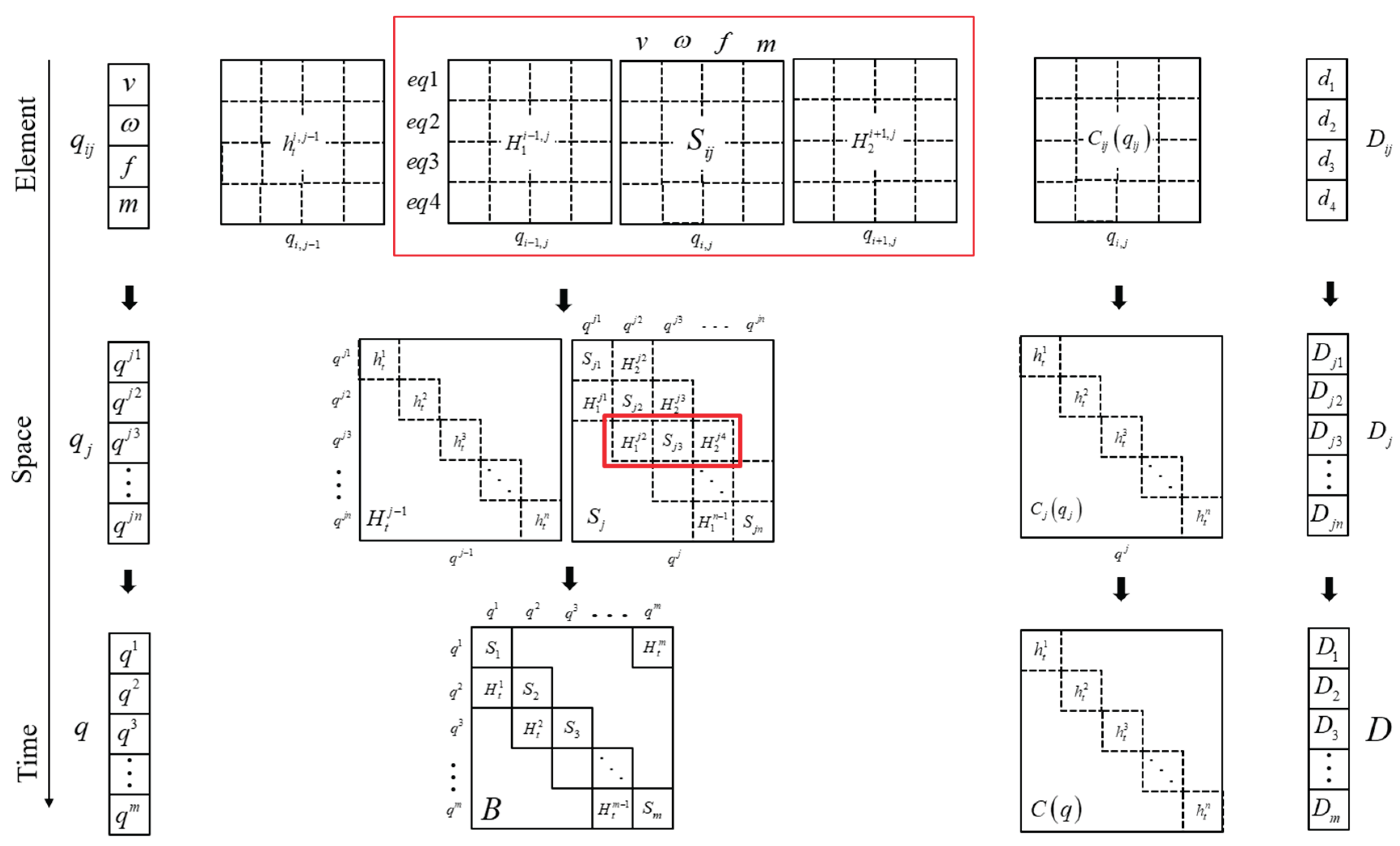
Figure 3.
Tip displacement diagram of cantilever under non-conservative tip force.
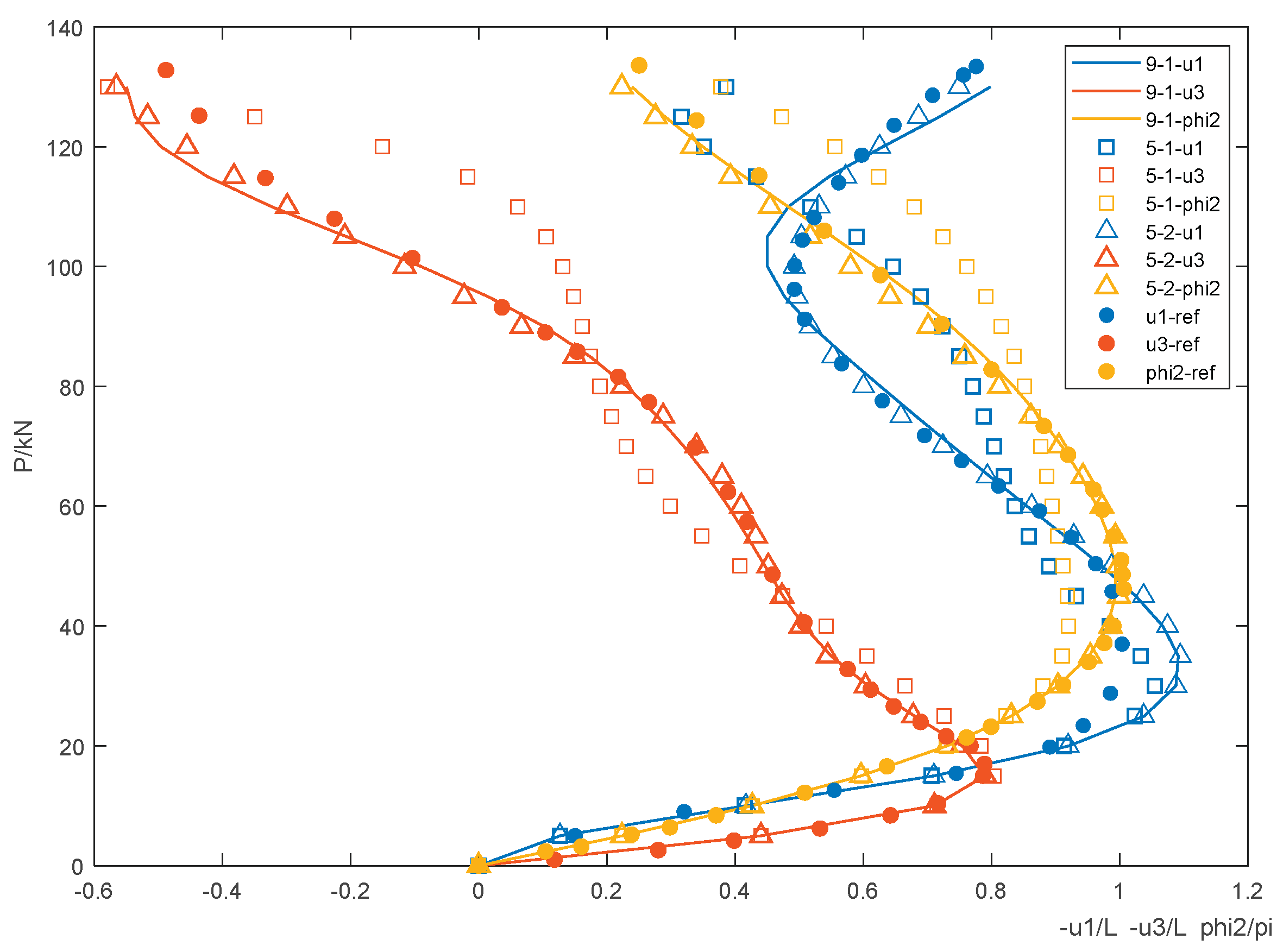
Figure 4.
Tip displacement diagram of cantilever under conservative tip force.
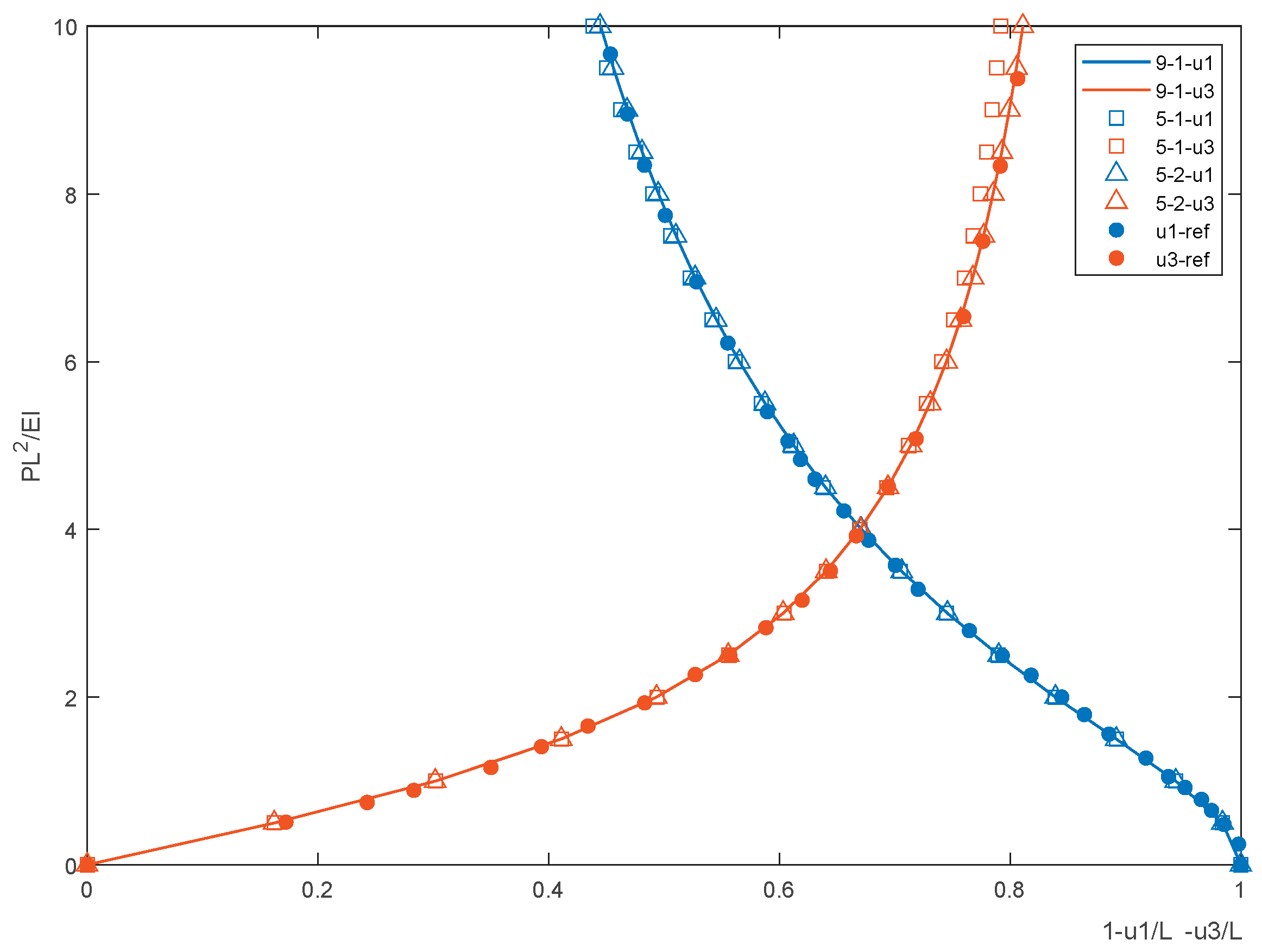
Figure 5.
Tip Displacements for a [0/90]3s Beam with different tip load.
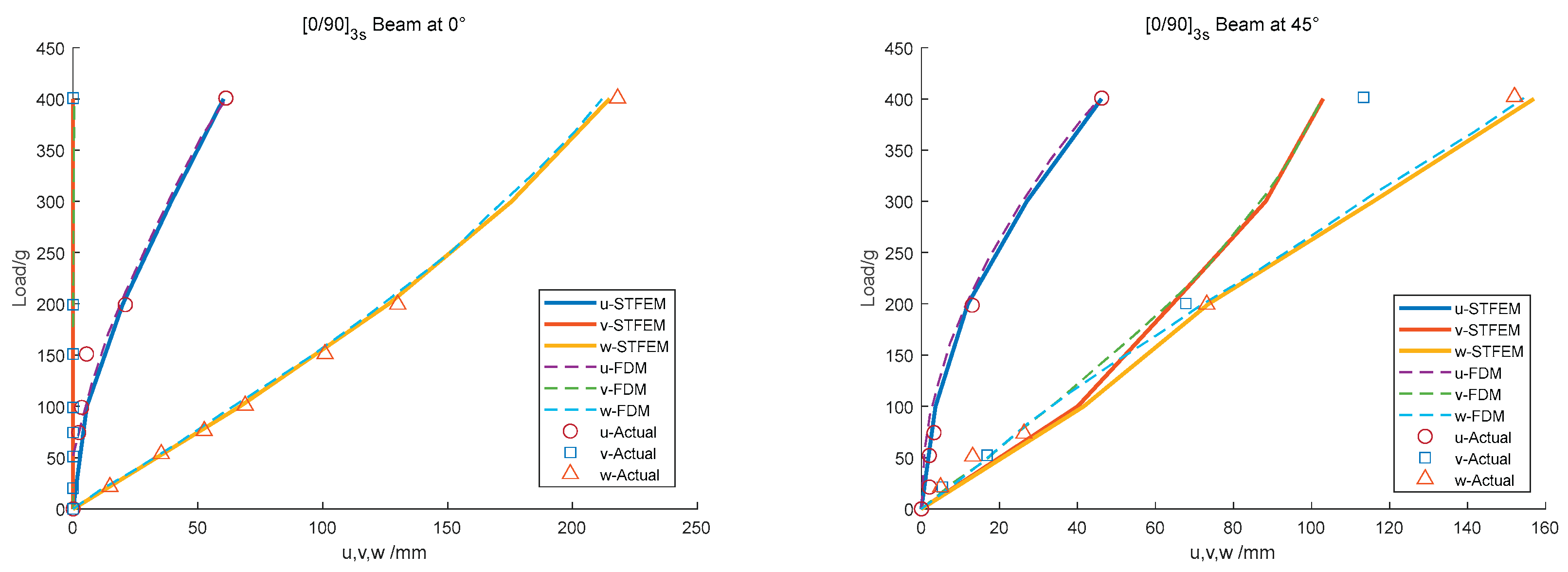
Figure 6.
Tip Displacements for a [45/0]3s Beam with different tip load.
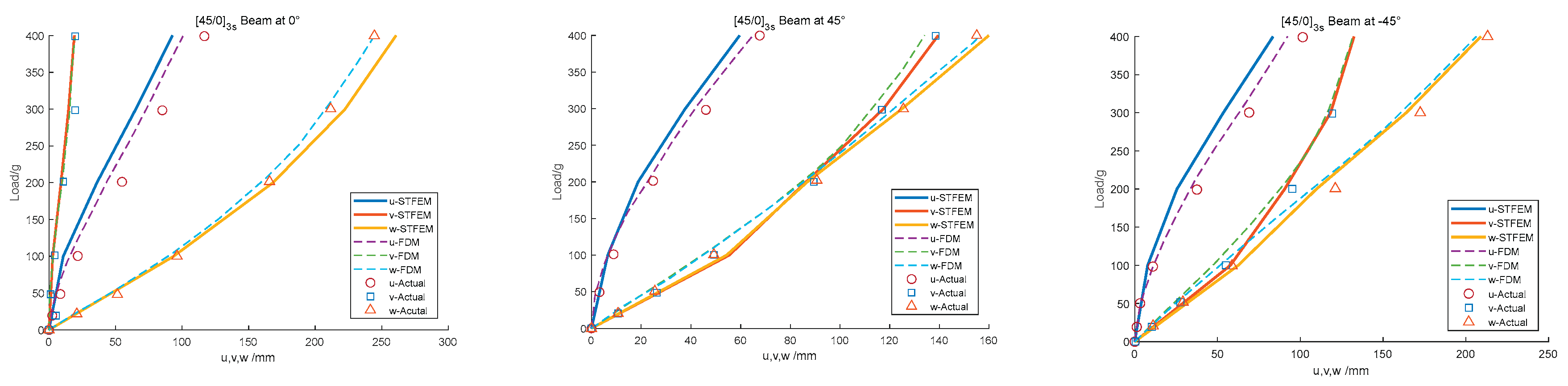
Figure 7.
Tip Displacements for a [20/-70/-70/20]2a Beam with different tip load.
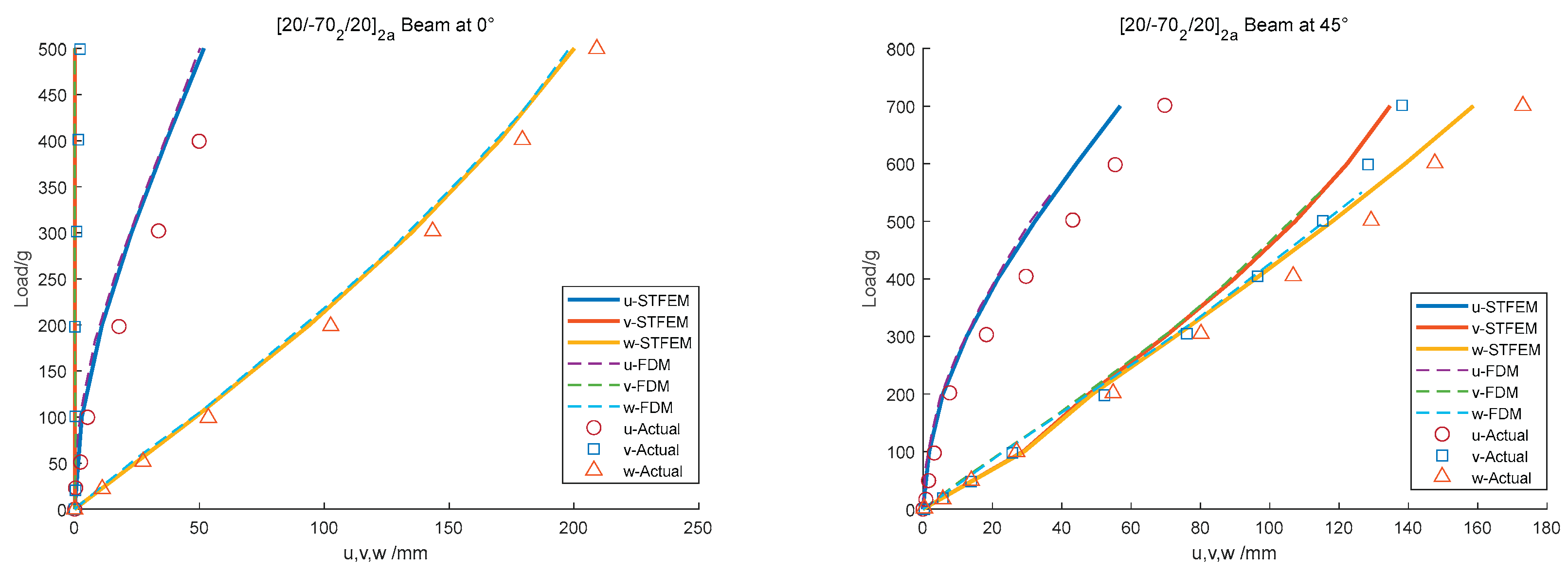
Figure 8.
Tip displacements (m) history with non-rotating for tip load F3=10sin(20t).
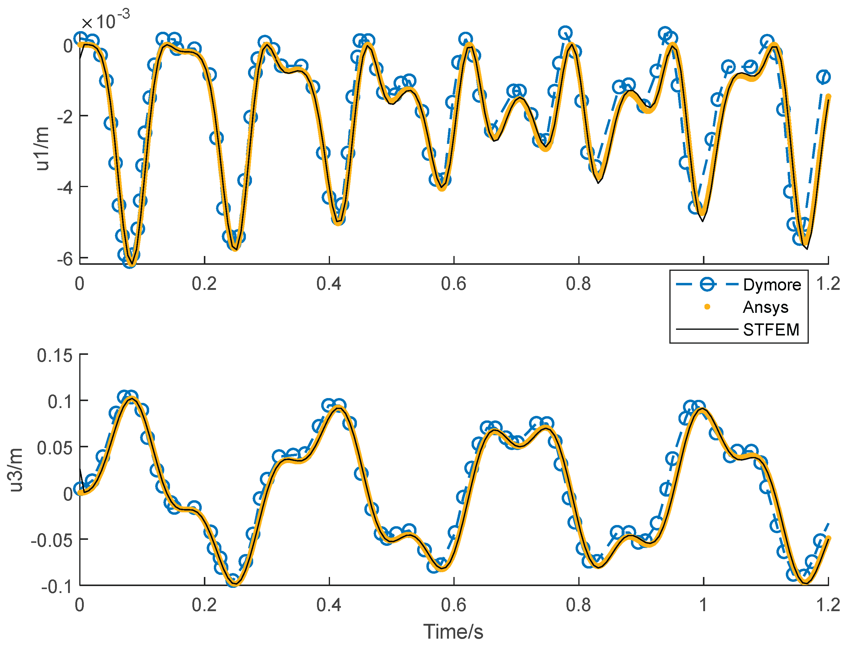
Figure 9.
Tip rotations (degree) history with non-rotating for tip load F3=10sin(20t).
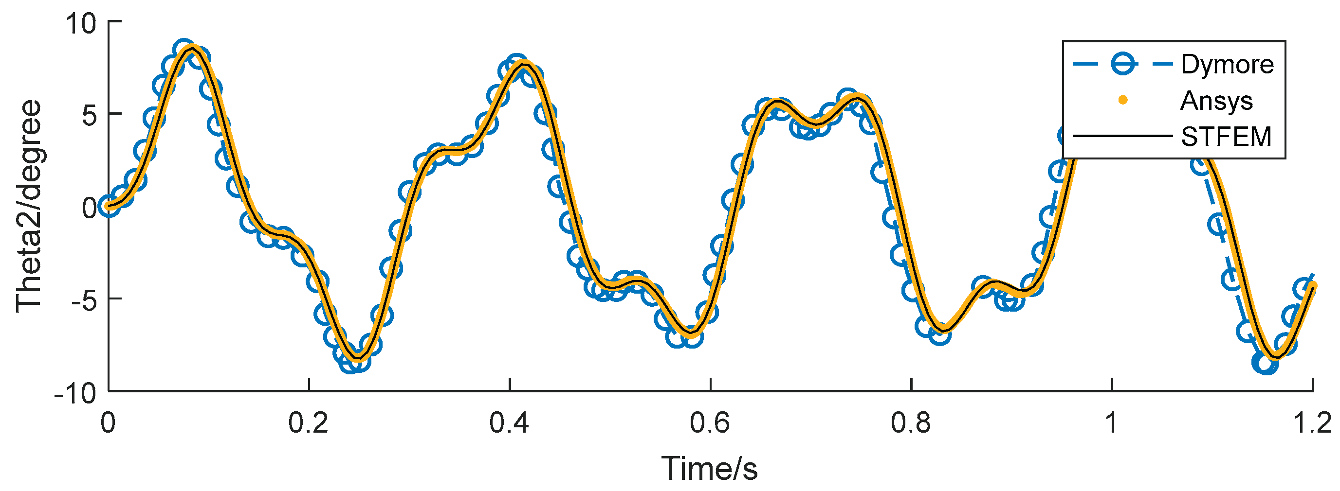
Figure 10.
Root forces (N) history with non-rotating for tip load F3=10sin(20t).
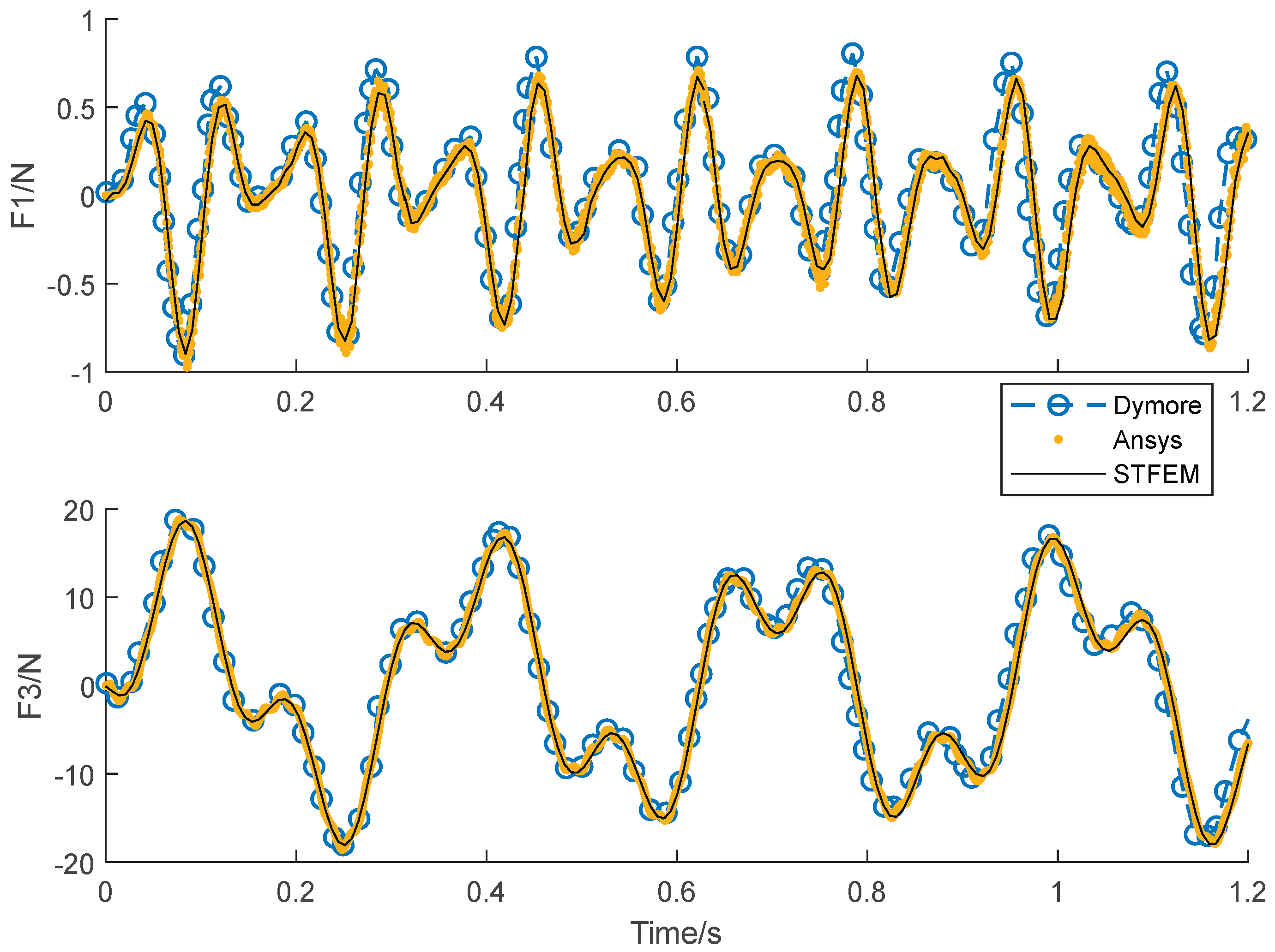
Figure 11.
Root moments (Nm) history with non-rotating for tip load F3=10sin(20t).
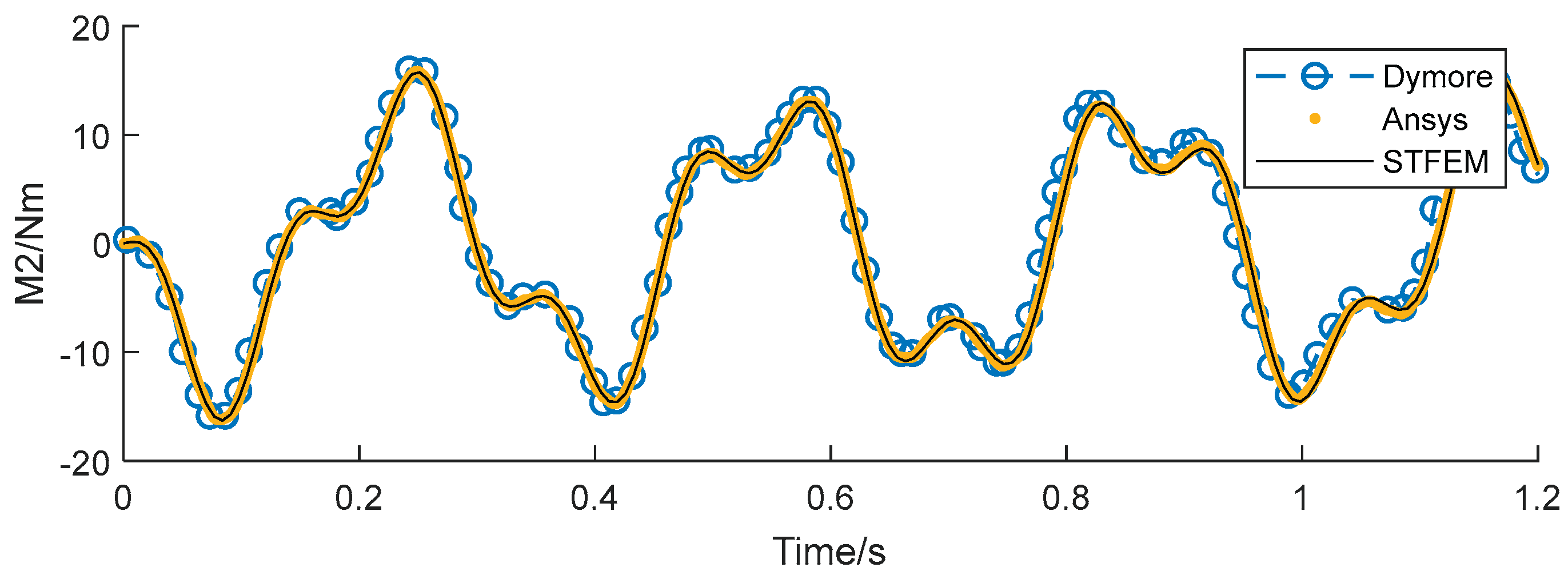
Figure 12.
Tip displacements (m) history with rotating for tip load F3=10sin(20t).
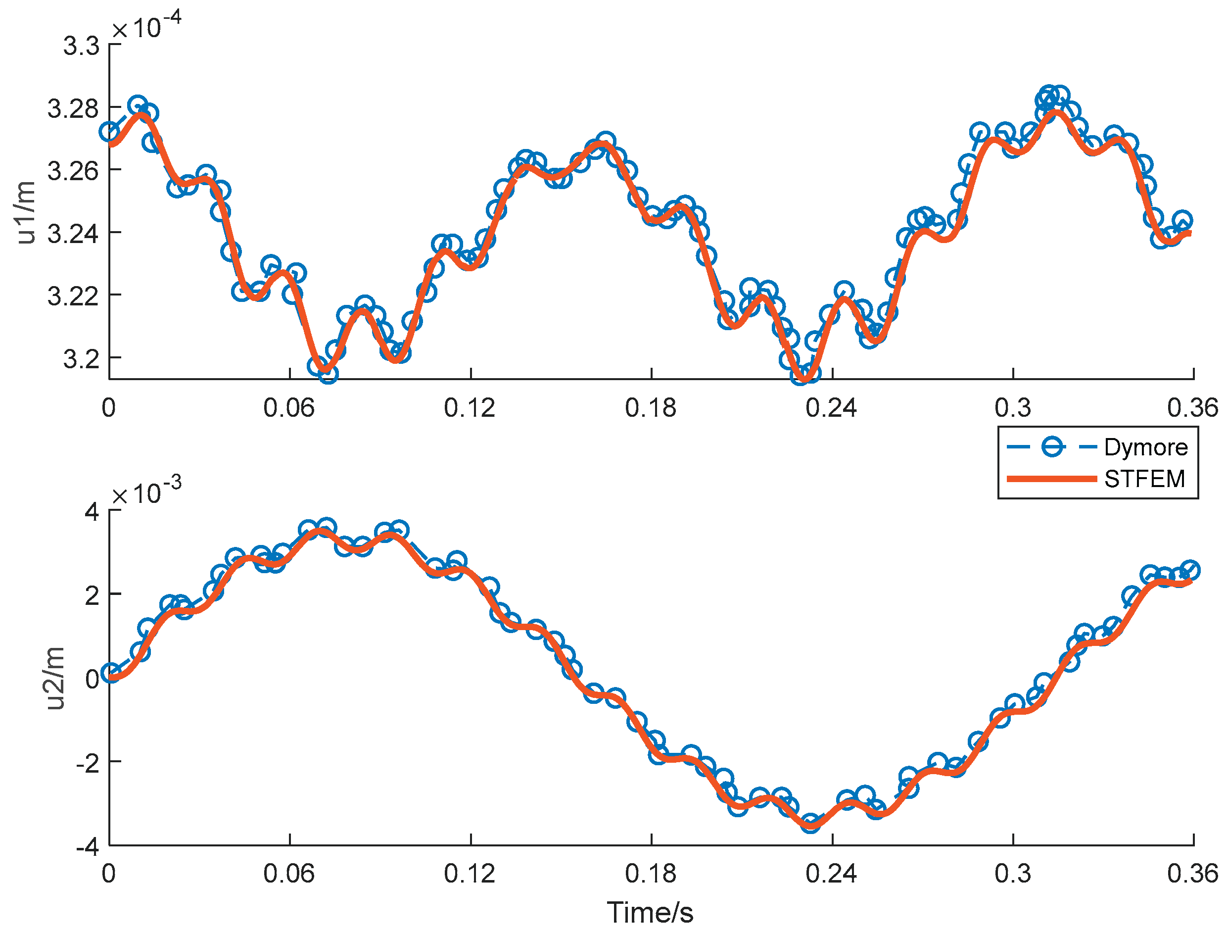
Figure 13.
Tip rotations (degree) history with non-rotating for tip load F3=10sin(20t).
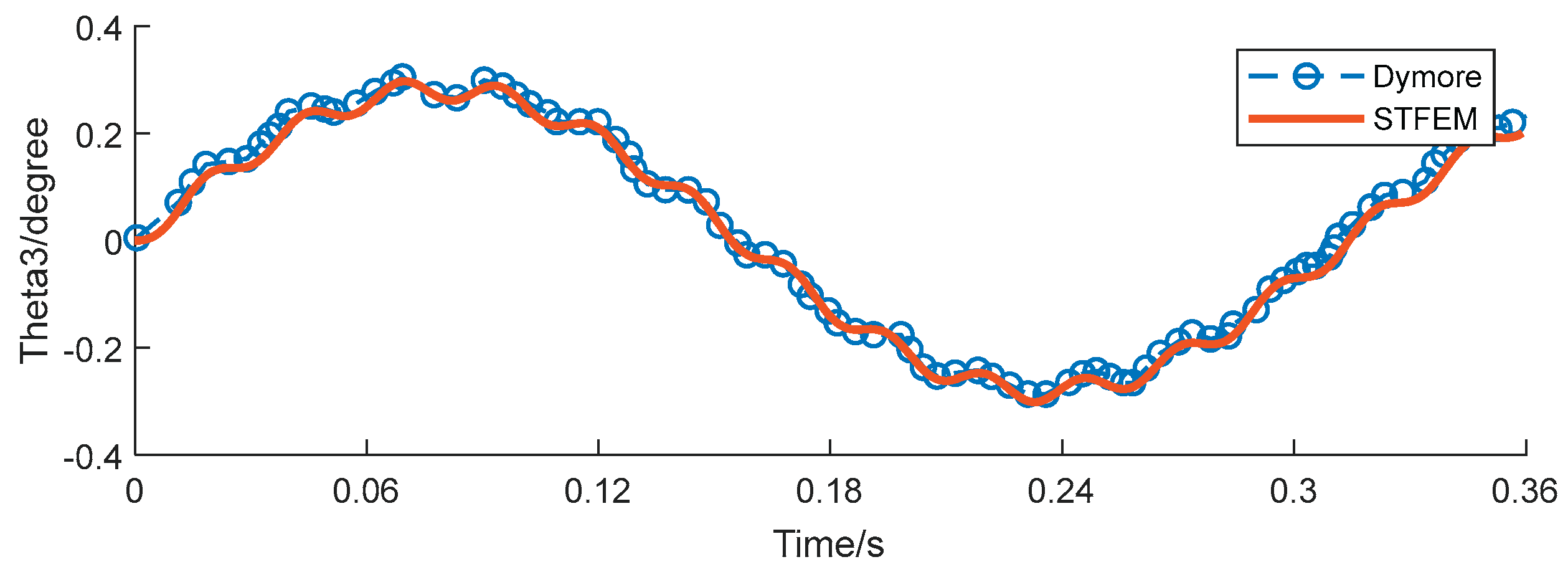
Figure 14.
Root forces (N) history with non-rotating for tip load F3=10sin(20t).
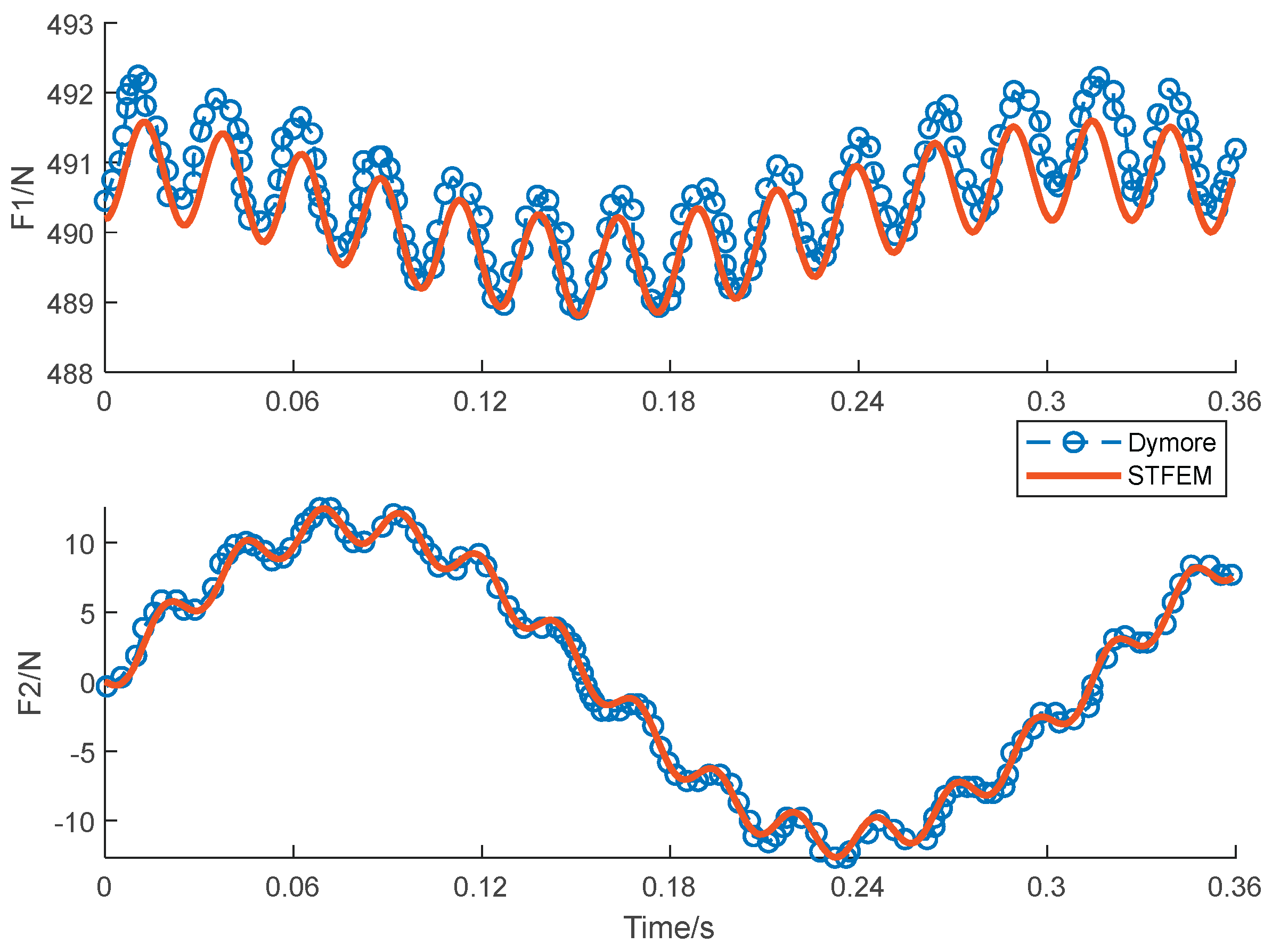
Figure 15.
Root moments (Nm) history with non-rotating for tip load F3=10sin(20t).
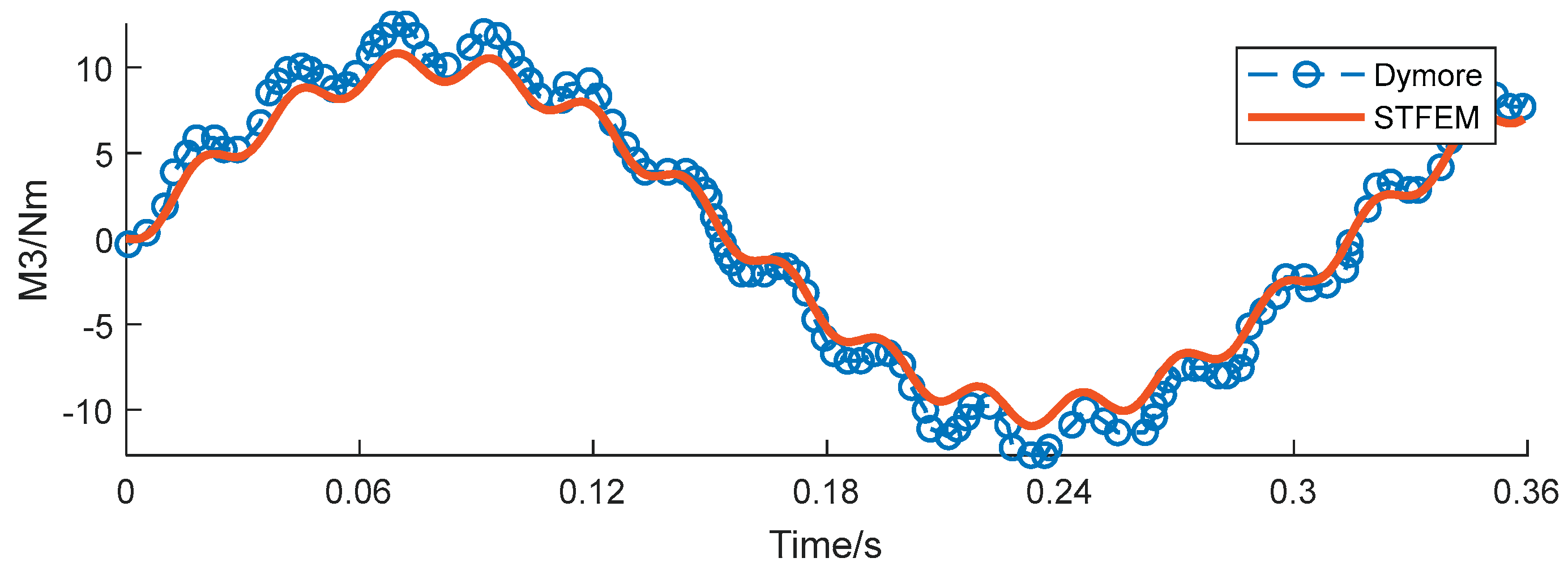

Table 1.
The tip position r3 of 9th order 1 element scheme vs tip bending moments.
| Moment / ft-lb | Exact / ft | This Paper / ft | Difference |
| 500 | 10.01401161 | 10.01401271 | 1e-6 |
| 1000 | 14.45688804 | 14.45698141 | 9e-5 |
| 1500 | 11.89004259 | 11.88999814 | 4e-5 |
| 2000 | 5.69137385 | 5.69011989 | 1e-3 |
| 2500 | 0.91168882 | 0.91032515 | 1e-3 |
Table 2.
The tip position r3 of 2nd and 9th order scheme vs elements number under 2500lb-ft2.
| Element number | 9th order / ft | Difference | 2nd order / ft | Difference |
| 1 | 0.91032515 | 1e-3 | / | / |
| 3 | 0.91166763 | 2e-5 | 0.91165092 | 4e-5 |
| 5 | 0.91169091 | 2e-6 | 0.91168341 | 5e-6 |
| 10 | 0.91168966 | 8e-7 | 0.91168634 | 2e-6 |
| 20 | 0.91168896 | 1e-7 | 0.91168896 | 1e-7 |
Table 3.
Material properties of the beam.
| Parameter | Value |
| Mass per unit length | 0.2 kg/m |
| Moment of inertia per unit length | 10−4 kg·m |
| Moment of inertia per unit length | 10−6 kg·m |
| Moment of inertia per unit length | 10−4 kg·m |
| Extensional rigidity | 106 N |
| Shear rigidity | 1020 N |
| Shear rigidity | 1020 N |
| Torsional rigidity | 50 N·m2 |
| Bending rigidity | 50 N·m2 |
| Bending rigidity (chordwise) | 1000 N·m2 |
Disclaimer/Publisher’s Note: The statements, opinions and data contained in all publications are solely those of the individual author(s) and contributor(s) and not of MDPI and/or the editor(s). MDPI and/or the editor(s) disclaim responsibility for any injury to people or property resulting from any ideas, methods, instructions or products referred to in the content. |
© 2025 by the authors. Licensee MDPI, Basel, Switzerland. This article is an open access article distributed under the terms and conditions of the Creative Commons Attribution (CC BY) license (http://creativecommons.org/licenses/by/4.0/).
Copyright: This open access article is published under a Creative Commons CC BY 4.0 license, which permit the free download, distribution, and reuse, provided that the author and preprint are cited in any reuse.


