
Submitted:
04 August 2025
Posted:
05 August 2025
You are already at the latest version
Abstract
Frequency-Modulated Continuous Wave (FMCW) Laser Detection and Ranging (LiDAR) systems have been widely utilized for their high accuracy and high resolution. However, traditional distance extraction methods often suffer from insufficient robustness in high-noise and complex background environments. To address this issue, this manuscript proposes a deep learning-based signal information extraction method that integrates a Dual Convolutional Neural Network (DCNN) with a Transformer model to enhance system performance. The DCNN employs multi-layer deep convolutions and pointwise convolutions to meticulously extract multi-scale spatial features, while the Transformer leverages the self-attention mechanism to efficiently capture the global temporal dependencies of the beat frequency signals. The proposed DCNN-Transformer network is applied to beat frequency signal inversion experiments at various distances. Experimental results on the test dataset covering a ranging distance from 3m to 40m demonstrate that the proposed method achieves a mean absolute error (MAE) of 4.1mm and a root mean square error (RMSE) of merely 3.08mm. The results indicate that our method is capable of achieving excellent prediction stability and high accuracy, exhibiting strong generalization capability and robustness for FMCW Lidar system.
Keywords:
FMCW LiDAR system
; deep learning
; deep convolutional neural network (DCNN)
; transformer
; signal processing
1. Introduction
With the rapid advancement of Laser Detection and Ranging (LiDAR) technology [1,2], Frequency-Modulated Continuous Wave (FMCW) laser ranging systems [3,4] have attracted significant attention and found wide applications in fields such as autonomous driving [5], environmental monitoring [6], and topographic mapping [7], due to their outstanding high-precision ranging capabilities. Unlike traditional Time-of-Flight (ToF) LiDAR systems [8], FMCW LiDAR offers superior performance in terms of precision and signal-to-noise ratio by continuously modulating the frequency of the transmitted laser, which enables not only accurate range detection [9] but also velocity estimation through Doppler-shift analysis [10].
During the FMCW ranging process, the transmitted signal and the target-reflected signal experience an optical path difference . The two optical signals undergo interference within the interferometer to generate a beat-frequency signal . The characteristics of are intrinsically linked to the target range R and relative velocity v, making it possible to effectively extract critical information. However, beat signals are often severely corrupted by various noise sources in practical applications. Consequently, accurate signal detection and information extraction remain challenging.
Traditional signal processing methods, such as Fourier transform [11] and wavelet transform [12], can provide basic processing of FMCW signals. Several studies have proposed improved ranging algorithms based on traditional spectral analysis methods. These include techniques that combine frequency and phase estimation of the beat-signal to enhance distance measurement accuracy [13,14]. However, their performances are often unsatisfactory in high-noise environments and under complex background interference. Specifically, when the signal-to-noise ratio is low, conventional approaches fail to effectively capture key signal features, which significantly limits the detection accuracy and robustness of the system.
In recent years, deep learning techniques have shown significant promise in signal processing [15], particularly through architectures such as Convolutional Neural Networks (CNNs) and Transformers. These models, known for their strong feature extraction and pattern modeling capabilities, have achieved impressive results in diverse fields including image processing [16], speech recognition [17], and time-series signal analysis [18].
Building upon these successes, researchers have increasingly applied deep learning techniques to FMCW radar ranging tasks, seeking to address the limitations inherent in traditional spectral analysis methods. For instance, Park et al. [19] proposed a five-layer neural network that utilizes FFT-derived features and significantly reduces distance estimation errors. Sang et al. [20] introduced a CNN-based framework for sparse signal processing, which maintains high velocity estimation accuracy even under partial data loss. More recently, Cho et al. [21] developed a lightweight one-dimensional CNN with a frequency-shift reuse mechanism, enabling accurate distance estimation with minimal labeled data and reduced hardware cost. To sum up, these approaches highlighted the growing advantages of deep learning in FMCW radar applications, particularly in terms of accuracy, robustness, and adaptability to challenging environments.
Following the same routine and handing the issues of FMCW LiDAR, this investigation introduces a robust feature extraction method integrating the advantages of Deep Convolutional Neural Networks (DCNN) and Transformer models, which enables effective operation under complex backgrounds and high-noise interference.
2. Methodology
2.1. DCNN for Local Spectral Feature Extraction
In FMCW LiDAR, the range to a target is traditionally estimated by using the Fast Fourier Transform (FFT) to transform the beat-frequency signal to frequency domain and locating its dominant peak. Although FFT-based methods provide a straightforward mapping from spectral peak to distance, they are inherently limited in capturing more subtle patterns,such as side lobes, noise fluctuations, or multi-target interference ,presented in the full spectrum. CNNs are a widely adopted deep learning architecture. The core advantages of CNNs lie in two key properties: local connectivity and weight sharing. To exploit these properties for spectral analysis, a one-dimensional CNN (1D-CNN) is employed to automatically learn and extract discriminative spectral features. By sliding convolutional kernels along the frequency axis, the 1D-CNN can identify local spectral signatures, suppress noise, and aggregate multi-scale patterns indicative of target range. This deep convolutional feature extractor thus constitutes the first stage of our hybrid architecture, enabling robust local representation of beat-frequency information before global modeling via the Transformer encoder.
In this study, building upon the conventional 1D-CNN, we design two parallel convolutional branches with complementary functions are designed at the front end of the network to simultaneously capture both coarse-grained and fine-grained features of the beat-frequency signals. This dual-branch structure enhances the network’s ability to model multi-scale spectral representations, which is essential for robust feature extraction under varying signal conditions.
The complete architecture of the proposed DT model is illustrated in Figure 1.
In the large-kernel branch, the first layer employs a one-dimensional convolution (Conv1d) with a kernel size of and a stride of 2 for downsampling, aiming to extract global pulse trends over a wide temporal window. This is followed by one-dimensional batch normalization (BatchNorm1d) and a learnable activation function (MetaAconC). Subsequently, another Conv1d layer with a kernel size of and a stride of 2 is applied to extract mid-scale features. To mitigate overfitting, a dropout layer (Dropout, ) is introduced thereafter. Finally, a one-dimensional max pooling layer (MaxPool1d) is applied to further aggregate the extracted features, to produce the final output of the large-kernel branch.
In the fine-grained branch, the spectrum is convolved sequentially with four 1D kernels of size , two with stride 1 and two with stride 2, while the channel dimensions evolve from 1, 50, 40, 30 to 30. Batch normalization and MetaAconC activations follow each convolution, and low-rate dropout () is applied after the final stride-2 convolution. Max-pooling (kernel size 2, stride size 2) is inserted after the second and fourth convolutions to resize the temporal resolution twice, yielding the output feature map of the branch.
After both branches complete downsampling to the same temporal scale, their output tensors are fused via element-wise multiplication across both the channel and time dimensions forming multi-scale coupled features.
The proposed DCNN feature extractor combines a large-kernel pathway, which captures coarse, global trends across the entire beat-frequency spectrum, with a fine-grained pathway that models detailed, local spectral patterns. By fusing these complementary representations through element-wise multiplication, the network produces a richly descriptive, multi-scale embedding of the FMCW beat signal. By fusing complementary representations, the network both discriminates true peaks from artifacts and improves robustness to interference, providing stable local features for the Transformer stage.
2.2. Integrating the Transformer into the DT Model
The Transformer model [22], known for its powerful modeling capacity, has demonstrated superior performance in long-sequence learning tasks, particularly excelling at handling complex temporal dependencies in sequential data [23]. The Transformer introduces the self-attention mechanism to compute dependencies between different positions within a sequence. The core idea of the self-attention mechanism is to capture the relationships among various elements in the sequence through a weighted summation, where the weights are adaptively learned attention scores.
We introduce the self-attention mechanism underlying the Transformer Block as preliminaries. Specifically, given an input sequence , where represents the input vector at the position, the attention mechanism can be calculated as follows:
where , , and denote the query, key, and value matrices, respectively, and is the dimensionality of the key vectors. This formulation describes how the attention weights are computed via the dot product between the query and key matrices, and how these weights are used to perform a weighted summation over the value matrix, thereby capturing the relationships and dependencies across different positions in the sequence.
To further enhance the model’s representation capability, the Transformer architecture incorporates a multi-head attention mechanism. Multi-head attention divides the query, key, and value matrices into h separate groups, computes attention independently within each group, and then concatenates the results. Assuming that the dimensionality of the queries, keys, and values in each head is , the multi-head attention can be formulated as:
where each attention head is calculated as:
This multi-head structure enables the model to jointly attend to information at different positions, which is critical for our global reasoning over DCNN-extracted features.
After DCNN multi-scale feature fusion, the resulting tensor is reshaped into a sequence of frequency-bin embeddings and fed into a Transformer encoder for global spectral modeling.
In our implementation, the fused feature map—arranged as a sequence of frequency-bin embeddings—is first augmented with positional encodings to preserve the ordering of spectral lines. Thereafter, it traverses self-attention and position-wise feed-forward networks, each wrapped by residual connections and layer normalization.
By attending over all frequency positions, the Transformer is able to capture long-range correlations and contextual cues that extend well beyond the local receptive fields of the convolutional kernels. This global attention mechanism enables the network to highlight informative spectral peaks, suppress noise artifacts, and resolve closely spaced returns that would otherwise be indistinguishable. The enriched, context-aware representation produced by the Transformer is then collapsed via flattening and fed into the final fully connected layers for distance regression. In this way, the integration of the Transformer module empowers the DT model with both local feature sensitivity and global spectral reasoning, resulting in significant gains in robustness and accuracy for FMCW LiDAR ranging under real-world noise and interference conditions.
After passing through the Transformer encoder layers, the output feature sequence is first flattened into a one-dimensional vector to facilitate subsequent regression computation. This flattened representation is then processed by two fully connected layers. The first layer performs dimensionality reduction, and the second produces the final distance estimation.
3. Method Implementation
3.1. Dataset Construction
The raw data used in this study are collected from the FMCW laser ranging system as shown in Figure 2. In this system, a frequency-modulated continuous wave signal is transmitted, and the echo signal reflected from the target is received and mixed with the local oscillator signal to generate a beat-frequency signal, from which distance information can be extracted.
We collect beat-frequency signals at 64 distances (3m - 40m).Each beat-frequency sample is represented in the frequency domain as a vector, with preprocessing steps (e.g., windowing and zero-padding) applied to preserve spectral resolution and amplitude fidelity. These spectral features directly encode target distance and reflectivity.
The resulting dataset underpins the training of our DT model for robust target-distance estimation in low-SNR FMCW scenarios, providing a quantitative benchmark for deep learning–based signal analysis in practical FMCW laser-ranging systems.
3.2. Network Model Training
During the training process, the Smooth L1 Loss function [24] is employed as the regression loss for the proposed model. The loss function is defined as follows:
where x represents the error between the predicted value and the ground truth, i.e., . When the error is less than 1, the loss adopts a squared error form (similar to L2 loss), which emphasizes the precise fitting of small errors. When the error is greater than or equal to 1, the loss switches to an absolute error form (similar to L1 loss), avoiding excessive penalization of large errors.
Compared with the traditional Mean Squared Error (MSE), Smooth L1 Loss applies a linear penalty for large residuals (), improving robustness to outliers, while retaining a quadratic penalty for small residuals (), Smooth L1 Loss retains a quadratic penalty, to finely fit minor signal variations in the signal.
This balanced design allows the model to achieve an effective trade-off between accuracy and robustness, particularly improving performance when dealing with noisy signals and datasets containing outliers.
Table 1 summarizes the distance inversion procedure based on our DT model.
3.3. Hyperparameter Optimization
Figure 3 (a) illustrates the impact of the number of Transformer layers on model performance. The number of layers refers to the count of stacked Transformer modules, each consisting of two components: (1) the self-attention mechanism, which computes relationships among positions in the input sequence and generates weighted feature representations; and (2) the feedforward neural network, which applies nonlinear transformations to the outputs of the self-attention. Each layer learns distinct representations of the input data. As the number of layers increases, the model can capture more complex and higher-level features, making the choice of layer count critical to performance.
When the layer count is 2, the median performance metric is 0.68, but with a wide distribution, indicating large fluctuations in model performance and unstable training. Increasing the layers to 3 or 4 results in a slight decrease in the median performance metric, accompanied by a narrower distribution range, suggesting reduced variability and improved training stability. At 5 layers, the median metric reaches 0.66, but the distribution range broadens again, implying decreased stability. Finally, when the number of layers increases to 6, the median performance slightly drops to 0.64 with a narrow distribution, indicating the smallest performance fluctuations and the most stable training process.
Overall, as the number of layers increases, the training stability improves and fluctuations diminish; however, beyond three layers, median loss improvements become negligible, and further increases yield limited benefits. Thus, we select three layers as optimal, balancing accuracy and stability.
Figure 3b presents the effect of the number of attention heads on model performance. The number of heads denotes how many parallel attention sublayers operate on the input, enabling the model to capture diverse feature subspaces. Self-attention captures dependencies among different positions in the input sequence, and multi-head attention enables the model to attend to diverse subspaces of information in each layer. Each attention head learns different feature representations, so increasing the number of heads allows the model to capture a broader variety of features.
With 2 heads, the median loss is approximately 0.61, with a wide interquartile range(IQR) indicating high performance variability. When the number of heads increases to 3, the median loss rises slightly to 0.62, while the distribution narrows, suggesting reduced fluctuation but higher loss compared to 2 heads. Further increasing to 4 heads yields a median loss similar to that with 3 heads, but still with the presence of outliers and relatively high loss values.
The lowest median loss and narrowest IQR occur at 2 heads, indicating that additional heads do not improve and may harm the stability.
3.4. Training Strategies
In this study, multiple training strategies are employed to enhance training effectiveness, improve stability, and prevent overfitting. These strategies include learning rate scheduling, partial parameter freezing, and early stopping. Each strategy has a specific implementation method, and all of them enables more efficient training and better generalization performance.
3.4.1. Learning Rate Scheduling
The learning rate is a critical hyperparameter in neural network training. A learning rate that is too high may cause instability during training, while a rate that is too low can lead to slow convergence or getting trapped in local minima. We use a dynamic learning rate adjustment strategy, where a scheduler adjusts the learning rate based on the validation loss.
Specifically, the scheduler monitors the validation loss after each training epoch and adjusts the learning rate accordingly. When the loss is low, the scheduler decreases the learning rate to allow finer adjustments in later training stages. Conversely, when the loss is high, a higher learning rate is maintained to accelerate convergence. This approach facilitates rapid convergence in the early stages and gradual refinement later, avoiding premature convergence to suboptimal solutions.
3.4.2. Partial Parameter Freezing
To avoid overfitting or unnecessary computational burden at certain training stages, partial parameter freezing was applied. Once the validation loss falls below , we freeze selected layers to exclude them from backpropagation. This reduces the model’s degrees of freedom and enhances training efficiency. By freezing less important parts of the network, the remaining parameters can focus on learning critical features, further improving efficiency.
After freezing, we switch to AdamP [25],an adaptive optimizer with decoupled weight decay,to enhance the generalization on the remaining parameters.This effectively reduces unnecessary computation and helps the model focus on optimizing crucial parts, boosting training efficiency.
3.4.3. Early Stopping
To prevent overfitting and maintain generalization performance on the validation set, an early stopping mechanism is implemented. The core idea is to halt training if the validation loss does not significantly improve over a certain number of epochs, thereby reducing unnecessary computation.
In this study, early stopping is triggered once the validation loss dropped below . The mechanism monitored loss changes, and if no substantial improvement is observed within a specified epoch window, training is stopped. This strategy ensure that the model does not overfit the training data and effectively reduce computational costs.
Based on comprehensive hyperparameter tuning, the optimal model configuration is summarized in Table 2. This configuration maintains low test loss while achieving a favorable balance in computational resource consumption, demonstrating high efficiency.
3.5. Experimental Results and Analysis
Figure 4 illustrates the loss trajectories of the proposed DT model. In the early epochs, the loss on all datasets decreased rapidly, indicating that the model quickly adapted to and captured essential patterns in the data. As the number of training epochs increased, the loss reduction gradually plateaued, demonstrating that the model’s learning has approached saturation and its indicating convergence towards optimal performance.
The validation and test loss curves remain closely aligned, suggesting that the model performs consistently across these datasets without significant overfitting. In the later stages of training, the losses on the validation and test sets remain low and show no noticeable increase.
The inset panel offers a magnified view of the fine-grained fluctuations in the loss curves between approximately epochs 3800 and 4200. During this phase, slight discrepancies appear among training, validation, and test losses, further suggesting stable and well-generalized learning. Overall, the experimental results demonstrate that the model achieves consistently strong performance on the training, validation, and test datasets without evident signs of overfitting. The model initially learns rapidly and gradually stabilizes, with yielding low, consistent loss values across on both the validation and test sets, demonstrating robust generalization capability.
As shown in Figure 5, the blue dots represent the distance points predicted by the DT model, where the x-axis denotes the actual value and the y-axis denotes the predicted distance. Ideally, each point should lie on the diagonal line where the x and y values are equal, indicating that the predicted distance matches the true distance. The red curve is a second-order polynomial fitted to the predicted distance points, reflecting the overall trend of the predictions. The blue predicted values exhibit a clear linear distribution along the red fitted curve. Within the prediction range (3–40 m), the points are evenly distributed on both sides of the fitted curve, indicating that the model maintains good stability across the entire measurement range. The positive slope of the fitted curve, which is close to the 45-degree reference line (ideal prediction line), confirms that the model effectively captures the positive correlation between the true distance and the predicted values.
Most predictions are tightly aligned with the ground truth, indicating high accuracy and consistent performance across the measurement range. Notably, even at the extremities of the distance spectrum—both minimum and maximum values—the predictions remain smooth and consistent, with no abrupt deviations even at the extremes of the distance range. This is highlighting the model’s robustness and stability in handling signals with widely varying amplitude levels.
Quantitatively, the model achieves a mean absolute error (MAE) of just 4.1mm and a root mean square error (RMSE) of 3.08mm on the test set. Notably, the model also performs exceptionally well in the long-distance range (30–40m), demonstrating the effectiveness of multi-scale convolution in spatial feature extraction, and the Transformer’s capability in modeling long-range temporal dependencies via self-attention. Overall, the synergistic effect of DCNN and Transformer not only improves the efficiency of feature extraction from the signal but also enhances noise suppression in complex backgrounds, offering robust support for high-precision ranging in FMCW LiDAR systems under diverse application scenarios.
4. Conclusions
In this study, an innovative deep learning-based approach was proposed to overcome the limitations of FMCW LiDAR systems in high-precision distance measurement. By leveraging the complementary strengths of DCNN and Transformer architectures, the signal processing capabilities of FMCW LiDAR were significantly enhanced. Specifically, the DCNN efficiently extracts multi-scale spatial features through stacked depthwise and pointwise convolutions, thereby improving the representation of spectral information. Concurrently, the Transformer’s self-attention mechanism effectively captured temporal dependencies within beat frequency sequences, exhibiting strong performance in modeling long-range correlations.
Experimental results confirmed the effectiveness and robustness of the proposed DT model. The training process demonstrated rapid convergence, with tightly aligned and stable loss curves on both the validation and test sets, indicating minimal overfitting. Quantitative evaluations further demonstrated that the model achieves highly accurate distance predictions across a wide measurement range, maintaining strong generalization ability even in long-distance scenarios. These results showed the potential of the proposed method to support high-precision, robust distance estimation in practical FMCW LiDAR applications.
Acknowledgments
This work was supported by the Baima Lake Laboratory Joint Fund of Zhejiang Provincial Natural Science Foundation of China under Grant no. LBMHY25F030002, Zhejiang Provincial Natural Science Foundation of China under Grant no. LY23F050001, the Municipal Government of Quzhou under Grant no. 2024D012.
References
- Raj, T.; Hashim, F.H.; Huddin, A.B.; Ibrahim, M.F.; Hussain, A. A Survey on LiDAR Scanning Mechanisms. Electronics 2020, 9. [Google Scholar] [CrossRef]
- Behroozpour, B.; Sandborn, P.A.M.; Wu, M.C.; Boser, B.E. Lidar System Architectures and Circuits. IEEE Communications Magazine 2017, 55, 135–142. [Google Scholar] [CrossRef]
- Hariyama, T.; Sandborn, P.A.M.; Watanabe, M.; Wu, M.C. High-accuracy range-sensing system based on FMCW using low-cost VCSEL. Opt. Express 2018, 26, 9285–9297. [Google Scholar] [CrossRef] [PubMed]
- Ula, R.K.; Noguchi, Y.; Iiyama, K. Three-Dimensional Object Profiling Using Highly Accurate FMCW Optical Ranging System. J. Lightwave Technol. 2019, 37, 3826–3833. [Google Scholar] [CrossRef]
- Li, Y.; Ibanez-Guzman, J. Lidar for Autonomous Driving: The Principles, Challenges, and Trends for Automotive Lidar and Perception Systems. IEEE Signal Processing Magazine 2020, 37, 50–61. [Google Scholar] [CrossRef]
- Sun, L.; Zhang, Y.; Ouyang, C.; Yin, S.; Ren, X.; Fu, S. A portable UAV-based laser-induced fluorescence lidar system for oil pollution and aquatic environment monitoring. Optics Communications 2023, 527, 128914. [Google Scholar] [CrossRef]
- Du, M.; Li, H.; Roshanianfard, A. Design and experimental study on an innovative UAV-LiDAR topographic mapping system for precision land levelling. Drones 2022, 6, 403. [Google Scholar] [CrossRef]
- Ma, J.; Zhuo, S.; Qiu, L.; Gao, Y.; Wu, Y.; Zhong, M.; Bai, R.; Sun, M.; Chiang, P.Y. A review of ToF-based LiDAR. Journal of Semiconductors 2024, 45, 101201. [Google Scholar] [CrossRef]
- Piotrowsky, L.; Jaeschke, T.; Kueppers, S.; Siska, J.; Pohl, N. Enabling High Accuracy Distance Measurements With FMCW Radar Sensors. IEEE Transactions on Microwave Theory and Techniques 2019, 67, 5360–5371. [Google Scholar] [CrossRef]
- Na, Q.; Xie, Q.; Zhang, N.; Zhang, L.; Li, Y.; Chen, B.; Peng, T.; Zuo, G.; Zhuang, D.; Song, J. Optical frequency shifted FMCW Lidar system for unambiguous measurement of distance and velocity. Optics and Lasers in Engineering 2023, 164, 107523. [Google Scholar] [CrossRef]
- Kim, C.; Jung, Y.; Lee, S. FMCW LiDAR system to reduce hardware complexity and post-processing techniques to improve distance resolution. Sensors 2020, 20, 6676. [Google Scholar] [CrossRef] [PubMed]
- Chen, Y.; Wang, J.; Li, G. A efficient predictive wavelet transform for LiDAR point cloud attribute compression. In Proceedings of the 2022 IEEE International Conference on Visual Communications and Image Processing (VCIP). IEEE; 2022; pp. 1–5. [Google Scholar]
- Ikram, M.Z.; Ahmad, A.; Wang, D. High-accuracy distance measurement using millimeter-wave radar. In Proceedings of the 2018 IEEE Radar Conference (RadarConf18); 2018; pp. 1296–1300. [Google Scholar] [CrossRef]
- Scherhäufl, M.; Hammer, F.; Pichler-Scheder, M.; Kastl, C.; Stelzer, A. Radar Distance Measurement With Viterbi Algorithm to Resolve Phase Ambiguity. IEEE Transactions on Microwave Theory and Techniques 2020, 68, 3784–3793. [Google Scholar] [CrossRef]
- Moysis, L.; Iliadis, L.A.; Sotiroudis, S.P.; Boursianis, A.D.; Papadopoulou, M.S.; Kokkinidis, K.I.D.; Volos, C.; Sarigiannidis, P.; Nikolaidis, S.; Goudos, S.K. Music deep learning: deep learning methods for music signal processing—a review of the state-of-the-art. Ieee Access 2023, 11, 17031–17052. [Google Scholar] [CrossRef]
- Archana, R.; Jeevaraj, P.E. Deep learning models for digital image processing: a review. Artificial Intelligence Review 2024, 57, 11. [Google Scholar] [CrossRef]
- Kim, S.; Gholami, A.; Shaw, A.; Lee, N.; Mangalam, K.; Malik, J.; Mahoney, M.W.; Keutzer, K. Squeezeformer: An Efficient Transformer for Automatic Speech Recognition. In Proceedings of the Advances in Neural Information Processing Systems; Koyejo, S.; Mohamed, S.; Agarwal, A.; Belgrave, D.; Cho, K.; Oh, A., Eds. Curran Associates, Inc., Vol. 35; 2022; pp. 9361–9373. [Google Scholar]
- Gao, Z.; Dang, W.; Wang, X.; Hong, X.; Hou, L.; Ma, K.; Perc, M. Complex networks and deep learning for EEG signal analysis. Cognitive Neurodynamics 2021, 15, 369–388. [Google Scholar] [CrossRef] [PubMed]
- Park, K.E.; Lee, J.P.; Kim, Y. Deep Learning-Based Indoor Distance Estimation Scheme Using FMCW Radar. Information 2021, 12. [Google Scholar] [CrossRef]
- Sang, T.H.; Tseng, K.Y.; Chien, F.T.; Chang, C.C.; Peng, Y.H.; Guo, J.I. Deep-Learning-Based Velocity Estimation for FMCW Radar With Random Pulse Position Modulation. IEEE Sensors Letters 2022, 6, 1–4. [Google Scholar] [CrossRef]
- Cho, H.; Jung, Y.; Lee, S. FMCW Radar Sensors with Improved Range Precision by Reusing the Neural Network. Sensors 2024, 24. [Google Scholar] [CrossRef] [PubMed]
- Vaswani, A.; Shazeer, N.; Parmar, N.; Uszkoreit, J.; Jones, L.; Gomez, A.N.; Kaiser, L.u.; Polosukhin, I. Attention is All you Need. In Proceedings of the Advances in Neural Information Processing Systems; Guyon, I.; Luxburg, U.V.; Bengio, S.; Wallach, H.; Fergus, R.; Vishwanathan, S.; Garnett, R., Eds. Curran Associates, Inc., Vol. 30. 2017. [Google Scholar]
- Beltagy, I.; Peters, M.E.; Cohan, A. Longformer: The Long-Document Transformer. 2020. [Google Scholar] [CrossRef]
- Girshick, R. Fast R-CNN. In Proceedings of the Proceedings of the IEEE International Conference on Computer Vision (ICCV), December 2015. [Google Scholar]
- Heo, B.; Chun, S.; Oh, S.J.; Han, D.; Yun, S.; Kim, G.; Uh, Y.; Ha, J.W. AdamP: Slowing Down the Slowdown for Momentum Optimizers on Scale-invariant Weights. 2021, arXiv:cs.LG/2006.08217. [Google Scholar]
Figure 1.
Complete architecture of the DT model.
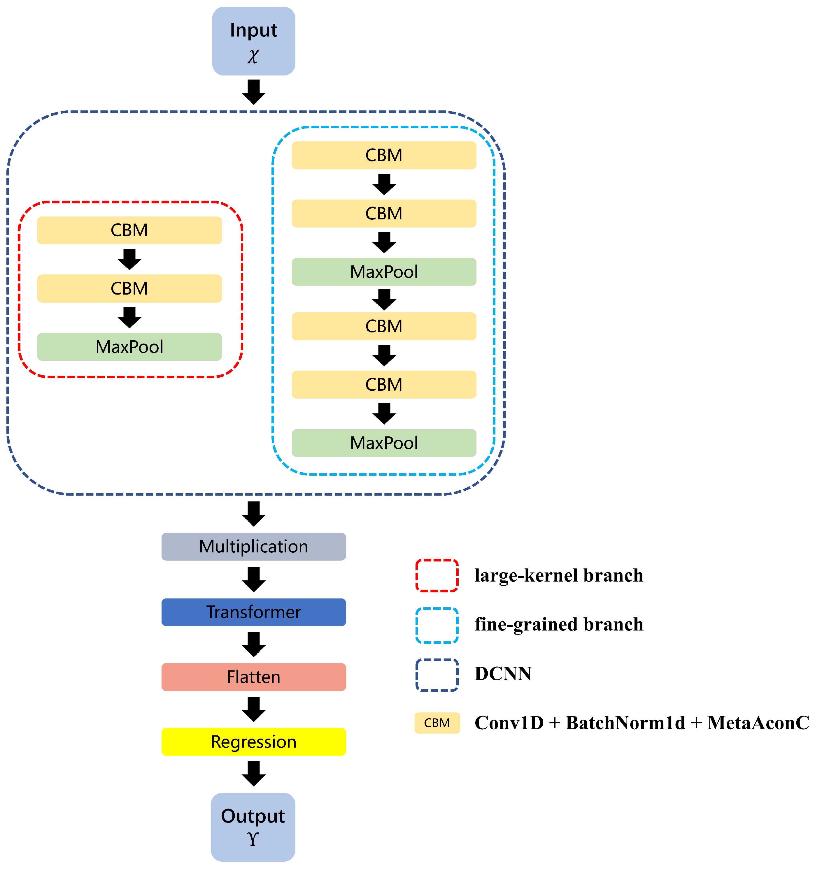
Figure 2.
FMCW LiDAR Ranging System.
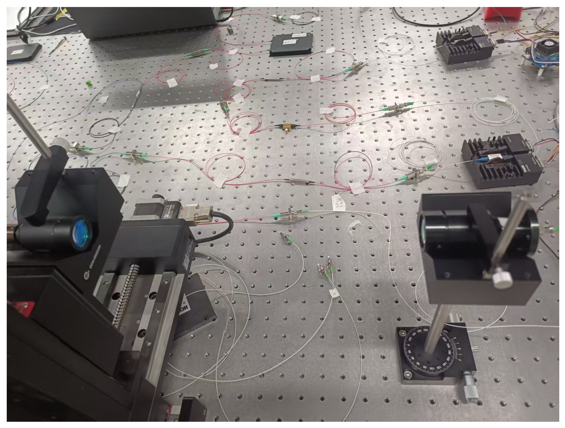
Figure 3.
Comparison of Transformer parameter optimization effects. (a) Number of layers; (b) Number of heads.
Figure 3.
Comparison of Transformer parameter optimization effects. (a) Number of layers; (b) Number of heads.
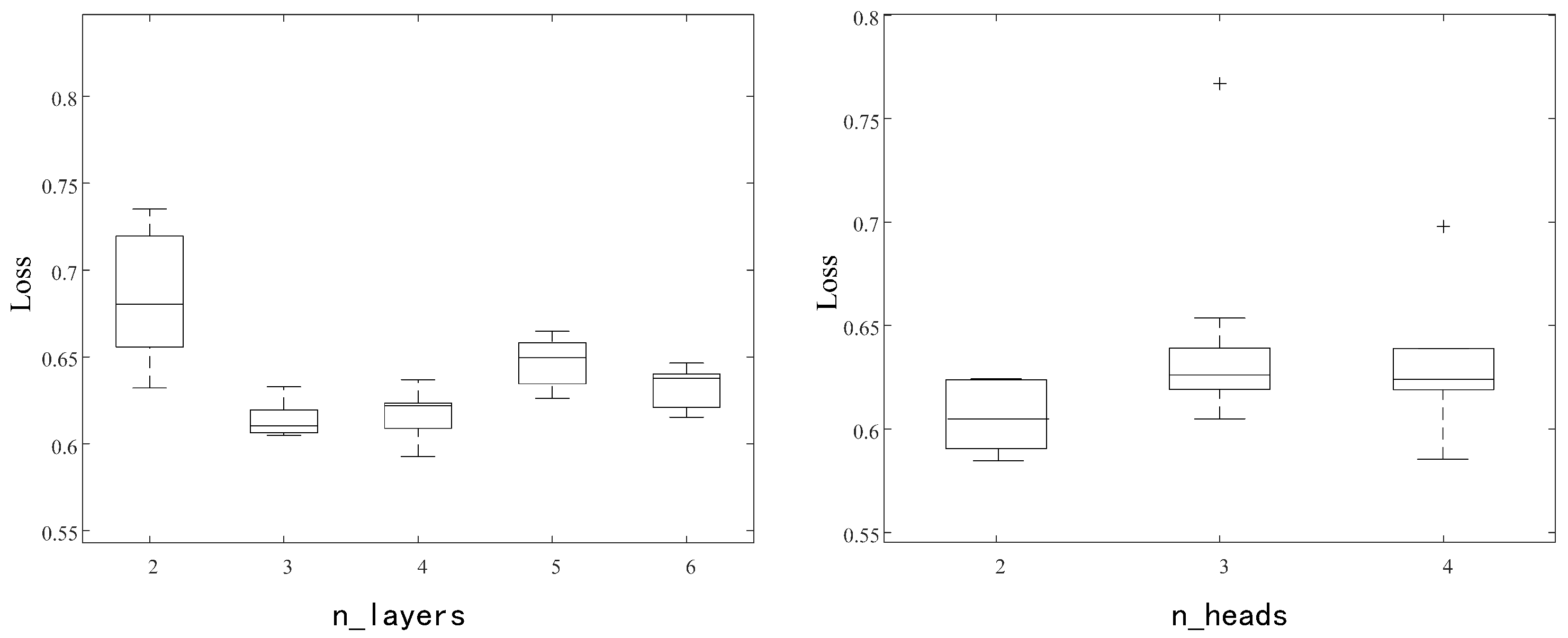
Figure 4.
Loss function curves of the DT Model.
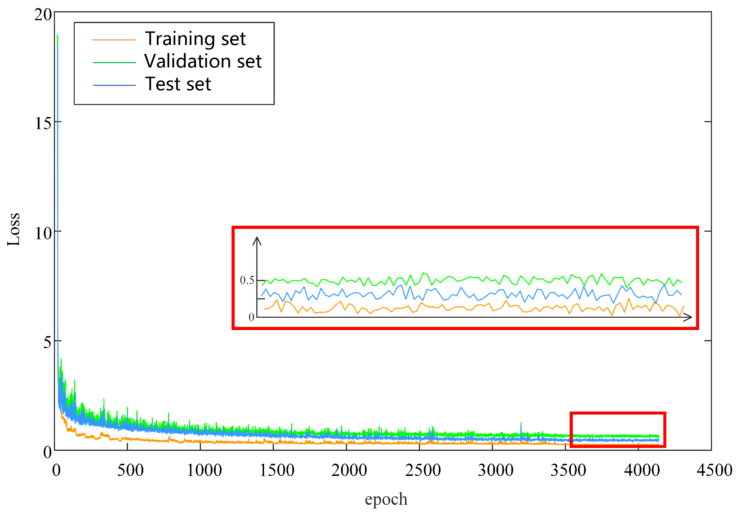
Figure 5.
Comparison between predicted and true values of the DT model.
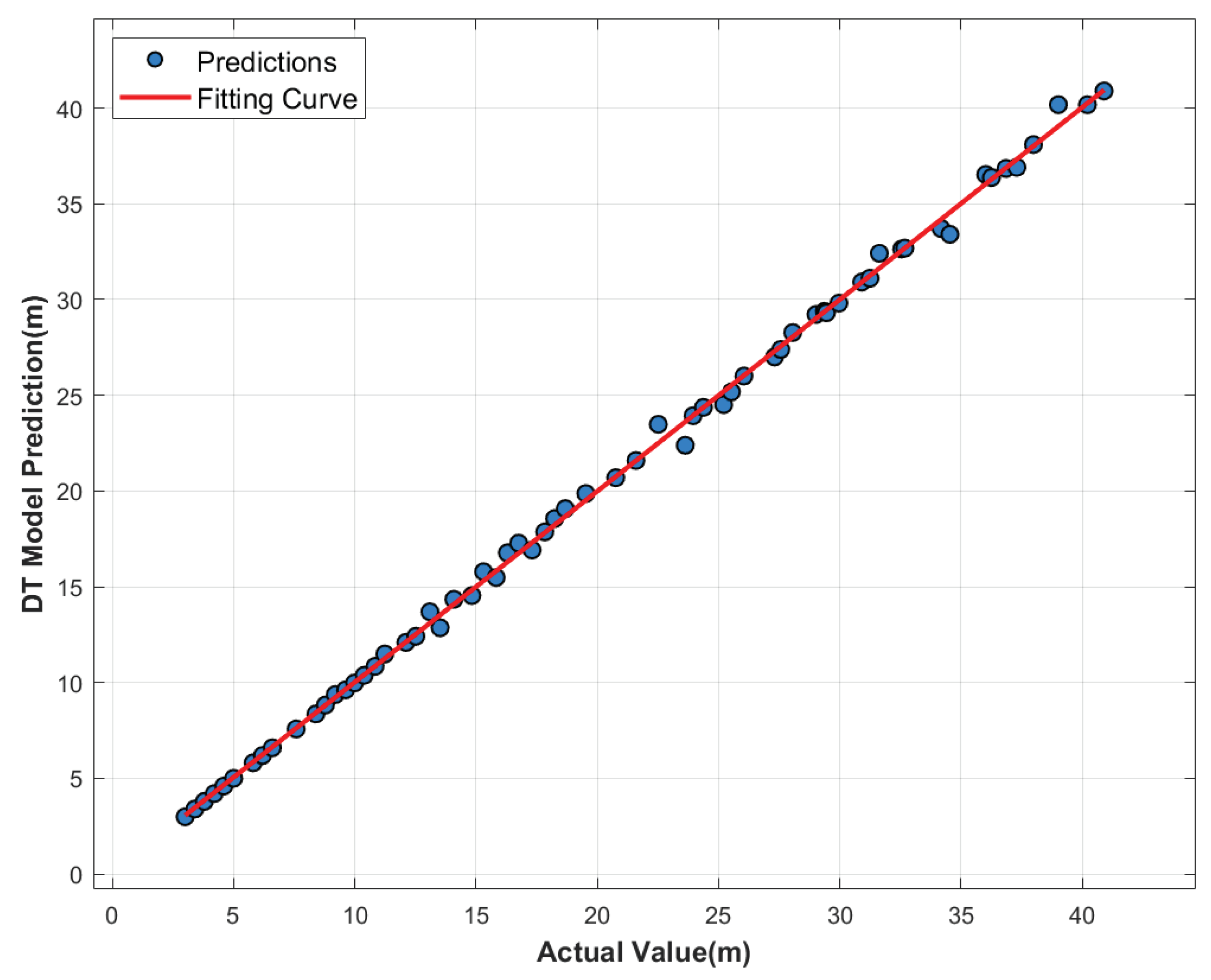

Table 1.
Training Procedure of DT Model.
| Step | Procedure | Step | Procedure |
|---|---|---|---|
| 1 | Load dataset | 13 | Validation phase |
| 2 | Dataset preprocessing | 14 | • Disable gradient computation |
| 3 | Data splitting (Train/Val/Test) | 15 | • Forward pass & loss on validation set |
| 4 | Model parameter initialization | 16 | • Record validation loss |
| 5 | Main Loop | 17 | Testing phase |
| 6 | Training phase | 18 | • Disable gradient computation |
| 7 | • Gradient management | 19 | • Forward pass & loss on test set |
| 8 | • Forward computation | 20 | • Record test loss |
| 9 | • Loss calculation | 21 | Learning rate adjustment |
| 10 | • Backpropagation | 22 | Layer freezing/optimizer reconfiguration |
| 11 | • Loss accumulation | 23 | Early stopping counter control |
| 12 | • Training loss recording | 24 | Loop Termination |
Table 2.
Hyperparameter List of DT Model.
| Hyperparameter Name | Value |
|---|---|
| Maximum Training Epochs | 5000 |
| Batch Size | 32 |
| Learning Rate | 0.00001 |
| Dropout Rate | 0.2 |
| Number of Transformer Layers | 3 |
| Number of Transformer Heads | 2 |
| Dimension of Q, K, V | 256 |
| Network Freezing Threshold | 0.0001 |
| Early Stopping Patience | 200 |
Disclaimer/Publisher’s Note: The statements, opinions and data contained in all publications are solely those of the individual author(s) and contributor(s) and not of MDPI and/or the editor(s). MDPI and/or the editor(s) disclaim responsibility for any injury to people or property resulting from any ideas, methods, instructions or products referred to in the content. |
© 2025 by the authors. Licensee MDPI, Basel, Switzerland. This article is an open access article distributed under the terms and conditions of the Creative Commons Attribution (CC BY) license (http://creativecommons.org/licenses/by/4.0/).
Copyright: This open access article is published under a Creative Commons CC BY 4.0 license, which permit the free download, distribution, and reuse, provided that the author and preprint are cited in any reuse.


