
Submitted:
23 December 2024
Posted:
24 December 2024
You are already at the latest version
Abstract
This work investigates the performance of different machine learning algorithms in the detection and identification of drones based on radar data from a 60 GHz millimeter-wave sensor. These signals are collected from a bionic bird and two drones, namely DJI Mavic and DJI Phantom 3 Pro, which were represented in complex form to hold amplitude and phase information. First benchmarks used four algorithms, namely LSTM, GRU, CNN, and Transformer, evaluated on noisy data. The main emphasis is on the assessment of algorithm robustness under noisy conditions, including artificial noise types like white noise, Pareto noise, impulsive noise, and multi-path interference. As expected, the Transformer outperformed other algorithms in accuracy, even on noisy data. However, certain noise contexts, especially Pareto noise, showed weaknesses in the effectiveness of the Transformer. For this purpose, we propose a Multimodal Transformer that incorporates more statistical features-skewness and kurtosis-in addition to amplitude and phase data. This resulted in a great improvement in the accuracy of detection, even under difficult noise conditions. Our results demonstrate the importance of noise in processing radar signals and the benefits afforded by a multimodal presentation of data in the problem of detecting UAVs and birds. The presented work sets up a benchmark for state-of-the-art machine learning methodologies for radar-based detection systems, providing valuable insight into methods of increasing the robustness of algorithms to environmental noise.
Keywords:
drone detection
; millimeter-wave radar sensor
; machine learning
1. Introduction
Drones or Unmanned Aerial Vehicle (UAV) are employed in an array of sectors nowadays. Although there are many advantages with UAV technology, the quick growth has also posed important issues of privacy and safety and security. These concerns have fueled the growth of the counter-UAV (C-UAV) market, ranging from military suppliers to innovative startups focused on detecting, tracking, identifying, and neutralizing unauthorized drones [1,2]. The challenge of detecting UAVs is particularly pronounced in environments where traditional sensors face limitations, such as low radar cross-section areas or during complex flight stages [3,4,5].
Several UAV detection methods have been explored in the literature, including acoustic monitoring [6,7,8,9,10,11,12], visible light [13,14,15,16,17,18], infrared [19,20], radar detection [21,22,23,24,25,26,27,28,29,30,31], and radio spectrum monitoring [32,33,34,35,36]. However, each method has its limitations. Acoustic monitoring is susceptible to ambient noise, and visible light detection can be impaired by weather conditions or obstacles such as buildings. As UAVs become smaller and less conspicuous, both infrared and radar technologies struggle to maintain their effectiveness.
An obvious one is radar detection, particularly millimeter-wave (mmWave) that complements the latter since it’s also more resistant to different weather conditions and provides high-resolution of detected objects. Besides, unlike the acoustic methods which may be influenced by environmental noise (such as city traffic or a crowd of people) and temperature activation threshold instability, radio waves always allow determine presence. radar is invariable to challenging natural conditions like rain and fog. This means acoustic detection is relegated to environments that can be well controlled, and impersonated best when simple and cheap; while infrared or computer vision techniques are only useful for scenarios with clear line-of-sight — both in stark contrast to the robust performance offered by radar across diverse operational contexts. RF monitoring can also be effective as a means of detecting RF-emitting devices, although it is at risk for being disrupted by random noise and other nearby RF emitters. In the end, radar’s dependability and high resolution also needs to be carefully considered for UAV detection across complex environment.
For smaller things with fine precision, the short-wavelength radars like mmWave radar sensors are chosen which is basically in 24 GHz to 300 GHz range and most common frequencies used are of 60GHz. One of the most important characteristics is for use in UAV detection, a significant requirement both from recreational and security points [23,28]. On the contrary, some issues like detection range and signal processing for mmWave radar are still hindering its effectiveness. Signal processing techniques and noise reduction methods are very important for maintaining the effectiveness of detection on high interference scenarios to overcome these challenges [29].
In this paper, we will discuss the 60 GHz millimeter-wave radar data collected by a bionic bird and two types of drones, DJI Mavic and DJI Phantom 3 Pro, applied to different machine learning algorithms. The performance of several models such as LSTM, GRU, CNN, and Transformer is compared, taking into consideration their robustness when noise is artificially added to the dataset. It has also proposed a Multimodal Transformer architecture based on amplitude, phase, skewness, and kurtosis features for better detection. It is aimed to enhance accuracy in a noise environment and will create a benchmark for more advanced processing techniques in radar-based UAV detection. However, in public safety, logistics, and agriculture, these findings are going to have very meaningful implications because identifying small drones for security and operational efficiency becomes increasingly critical.
2. Overview of Related Research
Recently, the detection and analysis of micro-Doppler signatures from UAVs, especially multi-rotor drones has received a lot attention. Yang et al. Yang et al. (2022) [21] provided a method to improve the rotor blade micro-Doppler parameters estimation through complex variational mode decomposition (CVMD), and singular value decomposition (SVD). It does well to get rid of some shortcomings in the traditional methods but it’s also not as good at getting accurate results when different speeds are used so obviously there is a context for going micro-motion parameter extraction based on it especially with multi-rotor UAV detection.
HHanif et al. (2022) [22] presented a comprehensive review of radar micro-Doppler signature analysis techniques, with a particular focus on target classification. Their work is about how the feature extraction has been evolving and what are the limitations of different approaches used until now. This provides a good background as small target detection — essentially the same problem model for classifying these drones or aerial targets.
Soumya et al. (2023) discussed recent advances in radar sensor technology focusing on mmWave radars [23]. Their review highlights the possible combination of radar data with machine learning algorithms for an improved overall performance in different applications including UAV detection. This inclusion of machine learning fits into our research approach to improve the way IRIS UAV detections can be completed with neural network models.
Kumawat et al. (2022) proposed a deep convolutional neural network (DCNN) for detection and classification of SUAVs via their micro-Doppler signatures [24]. Moreover, their dataset "DIAT-SAT" provides full radar signature information as well which can further enhance the accuracy of detection (especially in this domain). These efforts in under the hood DCNNs and custom datasets are close to our heart as we refine methods for UAV detection using radar data and emerging machine learning approaches.
Lu et al. (2024) [27] illustrate further advances in the detection using radar, where the use of exponential complex sinusoidal basis ( ECSB ) allowed for the extraction of micro-Doppler signatures to a high classification accuracy. Similarly, Kang et al. (2024) [28] provided valuable experimental data using 60 GHz mmWave for both drone and bionic bird micro-Doppler analysis by putting further emphasis on how accurate feature extraction is important in UAV detection.
A related study by Narayanan et al. (2023) [29] utilized TensorFlow in order to classify radar-based micro-Doppler spectrograms. The model resulted in very high accuracy when asked to differentiate between the drone types/birds. Their work thus further underlines the fact that the choice of robust classification models is an important consideration and constitutes one cornerstone of our approach for the detection of UAVs.
Lastly, Fan et al. (2023) [31] proposed a clutter suppression method using orthogonal matching pursuit, which effectively enhances the clarity of the micro-Doppler signal from environmental interference. This technique is especially relevant in improving the performance of detection under poor environmental conditions, and we hope to continue with such techniques in improving our methods of signal processing.
3. Foundational Theories and Methodological Approaches
3.1. The Detected Signal Representation
The radar signal model of multirotor UAVs is intrinsically based upon the interaction of radar with both rotor blades and the body of the drone. In this model, the reflected radar signal takes a specific form in micro-Doppler signatures. Indeed, those signatures are produced not only by the UAV itself but by the action of radar on flapping wings and bodies of birds. Mathematically, the micro-Doppler signal can be expressed as [27,31]:
where:
- L is a constant related to the radar system,
- is the wavelength of the transmitted radar signal,
- is the distance between the radar and the center of the UAV,
- P is the number of rotors on the UAV,
- K is the number of blades per rotor,
- is the Doppler phase associated with blade of rotor p,
- models the spatial response of the Doppler shift of each blade.
The formula is applicable to represent the signal captured by mmWave radar sensor datasets [25,28], considering that it has been fitted to the specific context of drone detection or similar objects and including micro-Doppler behavior in case of captured signal. The latter is a complex number array, which may be considered typical for the signals recorded by mmWave radar. These complex numbers encode the magnitude and phase of the reflected wave, both of which are basic to micro-Doppler calculations.
The key ingredients in the mathematical modeling of micro-Doppler include the following: L, a constant parameter associated with the radar system-the value that should be adjusted to conform to specific conditions of the radar setup. denotes the distance between radar and object-under-test - in our case, a drone - and determines the amplitude and phase of the complex data acquired. The other parameters are as follows: P denotes the number of rotors, while K denotes the number of blades per rotor; these two jointly determine the frequency modulation pattern observed in the radar signal.
-term is the interaction with the radar, which actually is the phase of the electromagnetic wave arriving back to the radar modulated by the distance from the radar to the object. It reflects the phase changes observed in the complex data. models phase modulation due to the movement of the rotor blades and gives the micro-Doppler signature typical for multirotor UAVs. This can also be interpreted as phase variation in the captured complex signal, whereby one notices changes continuously in both the real and imaginary parts with respect to time.
Although this is a formula that mathematically models an ideal situation, it captures all the main features in the behavior implicit in the radar data. However, the actual signal will be noisy, with fluctuations in environmental influence, several reflections, and disturbances around the sensor. In that aspect, filtering or any other noise separation techniques may be necessary to further refine the model and make full application to the context at hand.
3.2. Noise Models in the Original Signal Representation
Accurately introducing different types of noise to the modeling of radar signals is very important for enhancing both the reliability and precision of the model. Realistic radar signals are susceptible to different forms of noise; each has a different definition and depth of influence on the integrity of the signal.
White Noise usually is modeled as Gaussian noise and it represents the electronic noise intrinsic to the radar systems. It has a zero mean and a variance , mathematically described as:
It is the type of noise that, in the case of radar, interferes with signals’ clarity. This makes the whole process difficult to deal with, especially in regions that have high electronic interference.
Impulsive Noise: It is of a sporadic nature and comprises high-amplitude pulses; it can be modeled by a Poisson distribution with a rate :
Such noise may result from sudden interference, an electrical discharge, or an abrupt change in the source signal that masks and/or distorts the signal being transmitted by the radar.
Noise following the Pareto Distribution can be modeled as:
where and are parameters that define distribution. This noise has heavy tails. It can bring large, infrequent disturbances in the signal as representation of a rare event that can significantly impact radar data interpretation.
Multi-path interference: The reflection of radar signals from various surfaces to the receiver causes interference among several late-time copies of the same signal. This situation arises when surroundings contain high-rise buildings, or if the terrain is complex enough to alter significantly the waveform of the received signal. The resultant interference may degrade target detection or tracking due to error. Multipath noise can be modeled mathematically as follows:
where represents the magnitude of the multi-path component, is the transmitted radar signal, and is the time delay associated with each multi-path reflection.
It is very important to incorporate such kinds of noises into the model of the radar signal for an appropriate simulation of the diversity encountered in practical radars. With different noise types considered, the extended representation of the radar signal is given as:
This general model provides better processing and analysis of the signals, hence a good method for the detection and interpretation of radar data with many sources of noise and effects of interference. This model, since there will be one term to account for each type of noise, can accommodate myriad disturbances associated with radar signals. Finally, it offers a close approximation to actualities in the operation of radar hence offering robustness and more realistic accuracy in the representation of radar signals.
3.3. Machine Learning Algorithms for Drone Detection
Recent advances in signal processing and machine learning have considerably enhanced the performance of sensors in detecting UAVs [3,4,5]. Higher detection accuracy and reliability have, therefore, enabled the identification of small-sized drones that become relevant in many applications related to surveillance and recreational use, for example, [6,8,10,13,14,15,16,17,24,27,29,32,33,34,35]. These, integrated with radar systems, ensure superior spatial resolution and, more importantly, effective operations in difficult environmental conditions for more robust UAS detection solutions [21,22,23,24,27,29].
Several machine learning models are implemented to investigate their performances related to the detection and classification of UAVs. In particular, both LSTM networks [5,8,11,18] and GRU [11,18] have the particular advantageous capability of temporal dependency and sequential data handling. This is very important, as radar signals are time-series data and flying patterns of aerial objects are not steady in some conditions. It is also especially superior in the representation of the spatial hierarchies and local patterns that can be found in radar data. Therefore, it is able to effectively capture distinguishable features in decomposed signal components.
CNNs are really adept at catching such spatial hierarchies and local patterns in radar data, serving the purpose intrinsically for distinct feature identification from decomposed signal components [4,5,8,10,13,14,15,16,17,22,24,34,35]. Besides this, Transformer models are also employed for their ability to handle long-range dependencies and self-attention mechanisms with much greater efficiency [15,16]. These are highly crucial to understand the complex interaction within the radar signals themselves for correct classification. Among the selected algorithmic approaches, some bear respective strengths to address the nature of the data with a particular interest in sequential and spatial features to enhance overall performance and reliability for any given real-world scenario of detection and classification.
Many drone detection algorithms are based on machine learning methods applied either in conjunction with or as standalone alternatives to signal decomposition techniques [7,8,9,21,22,27,33] and attention mechanisms [13,15,16]. While the signal decomposition is applied quite often in the context of acoustic sensors and sometimes in the radar, the attention mechanisms are used more frequently in the case of visual sensor systems. Other methods rely on visualization techniques of the signals based on spectrograms [6,22,29,36] to detect and classify drone activities. Other approaches are simply statistical techniques [12,18,30,36], and signal analysis is performed with no machine learning involved.
While traditional methods are extremely efficient in analyzing patterns or trends within data, machine learning algorithms perform extremely well when modeling hard, nonlinear relationships that may not be as saliently evident by purely statistical means. Algorithms of this type are able to learn features automatically from enormous datasets, reducing the need for manual feature extraction.
Machine learning models can adapt and improve over time; thus, their functionality will be even better in environments that have much variability and challenge-even highly interfering or noisy ones. Unlike the visual signal methods, which may depend on specific patterns or thresholds, machine learning can generalize over different signal types and conditions, hence making the robustness and accuracy of drone detection better.
3.4. Overview of the Dataset Employed in This Research
Kang et al. (2024) [28] gives the radar signal collection collected through a 60 GHz radar sensor. This data structure falls within three dimensions, which are important for the working of the sensor and its interaction with the environment.
The first dimension stretches across 1000 entries, which represent distinct time instances or "frames" in temporal sequence capturing the motion or otherwise appearance of objects (drone, bird, etc.) present in the radar field of view. At a very high level, these frames represent the snapshots of scenes observed during one period running.
The second part has 128 subdivisions in each frame; those windows act as smaller time windows giving enhanced temporal resolution. This allows sensing the micro-Doppler phenomenon of rapid wing flapping or rotor motion, which is significant for classifying objects by type and activity.
The third dimension has 168 functional attributes acquired during each time window, including real and imaginary parts, amplitude, phase, and other properties of the radar signal, enabling an insightful view of the moving, shape and material properties of the target. This will allow for a proper training setup of machine learning models on object classification based on movement patterns or physical properties.
The dataset features hovering UAVs (e.g., Mavic series, Phantom 3 Professional) and a bionic bird, which are more difficult to detect due to small sizes of the radar cross section (RCS) and their composition in materials like carbon fiber and plastic that reflect a little radar energy [27]. Add to that the fact that these drones are hovering, making them more difficult to detect because they produce weak Doppler shifts. Simulated signals with overlaid noise will also further examine how pathologically close to natural such mimic systems could become.
4. Results
4.1. Introduction to the Results
It was this chapter which describes the outcome of an investigation into the detection and identification of drones using machine learning algorithms applied to 60 GHz millimeter-wave radar data. Collected Radar signals were analyzed with a bionic bird and two drones such as DJI Mavic and DJI Phantom 3 Pro under conditions in which artificial noises had been introduced. Major models like LSTM, GRU, CNN and Transformer have also been trained and evaluated just based on the competed noisy dataset in order to establish performance metrics such as accuracy and error rates for degraded environments.
Full imitated realistic operating conditions included full addition of white noise, Pareto noise, impulsive noise, and multipath interference. The boxplots present the data classification distribution, assuring demonstration of algorithm capability in being able to classify between classes; performance of the models was analyzed using ROC curves. Phase and amplitude data formed the prime input features for all models in this benchmark.
Furthermore we extended the dataset to add two more statistical features - kurtosis and skewness - to improve detection and overcome the challenge of noise. Hence used a Multimodal Transformer architecture integrating them with amplitude and phase data. This enhancement resulted in better classification accuracies as well as robustness against noise, hence presenting a more efficient and reliable method for radar-based UAV detection. This result brings to the fore the effectiveness of the proposed method in cases where noise notwithstanding performance is desirable.
4.2. Noisy Signal Visualization
This research discusses the effects of various noise patterns on mmWave radar signals, such as white noise, Pareto noise, impulsive noise, and multipath interference, which entails some parameters controlling their intensities and behaviors.
White Noise is determined by the noise factor parameter whose value is set equal to 10, indicating that it will multiply the standard deviations of the real and imaginary parts of the signal’s mean and add a Gaussian effect centered around the signal’s average.
For Pareto noise, in this case, the weight of the noise tail is defined by the alpha parameter with a value of 1.5 and by the noise factor with a value of 10, which indicates the deformation of the intensity toward relative correlativeness of the noise computed in relation to the standard deviation of the signal.
Impulsive Noise is modeled with impulse ratio of 1, thereby indicating that about 100% of the samples will be affected, and scale factor of 10, which is used to define the amplitude of the impulsive noise.
Multipath interferense is defined using specifiers number of paths (10 reflections), maximum delay (10 samples), and maximum intensity (10) to simulate reflections that have different delays and different intensities.
These noise models make a simulation of the real-world situation where interference occurs with the parameters chosen to reflect the average environment that radar systems might encounter.
In Figure 1, for amplitude, the white noise shows a well-defined range of values, while its interquartile range appears to be very narrow but is compensated with a significant number of high-magnitude outliers. These outliers signify that white noise contributes to the variability in the data, but most of the amplitude values are focused around the lower end. The presence of such extremes suggests that when signals get distorted in their dynamics, particularly in the amplitude domain, it would affect the later processing or modeling of data. Phase, as per the right box plot, seems to be less influenced as compared to the amplitude with white noise. The interquartile range is wide, with most values in a controlled range between approximately 1 and 3. Also, there are no extreme outliers in phase data, which indicates that the phase is relatively immune to white noise contaminations. Thus, white noise does not affect much with respect to degrading the phase information but allows it to be preserved for certain applications.
For Pareto noise, Figure 2, the amplitude (left) undergoes drastic changes from low levels of noise, as seen by a very broad range of values but also many outliers with very high magnitudes. Most of the data points tend to cluster around zero with little evidence of the interquartile range, which means that the noise had introduced a highly skewed distribution. This phenomenon is in accordance with the already known properties of Pareto noise which has proven to generate long-tails with extreme deviations. The phase (right) seems not to be disturbed by the Pareto noise so much. The interquartile range is well defined, with most values lying in a very limited range and having no visible outliers. This seems to indicate that at least the noise is affecting the phase a bit but in comparison to the amplitude, its effects are mild. The limited distribution signifies that perhaps the phase data can yet be somewhat interesting without going beyond what is needed for a model or an analysis.
The boxplots in Figure 3 show effects of impulsive noise on the amplitude component (left) and phase component (right) of radar signals. Amplitude-wise, impulsive noise causes high variability, with IQR clumped near low magnitudes, and median nearly bottom of the IQR. The most pronounced feature is denoting several extremely high outliers. These outliers show that impulsive noise severely deforms some amplitude data points, resulting in isolated spikes of very high error. Such behavior conveys that the impulsive noise contributes random but high amplitude deformations to the types of signals. The phase data seem to be quite resistant to impulsive noise, on the contrary. The IQR is broad; most values lie between approximately 1 and 3 in error magnitude. The median phase error is located well within the IQR, thus indicating a more consistent distribution. More importantly, the nonappearance of extreme outliers in the phase data means that impulsive noise affects the phase more uniformly, so it does not lead to deviation values that are excessively high. This is indicative of the robustness of the phase with regard to the sporadic high-intensity character of the impulsive noise as compared to the amplitude.
Under multipath interference, in Figure 4, the IQR is thus widely spread for magnitude errors. The median is a bit below the center of the IQR, indicating a slight skew towards lower values. The whiskers indicate a large error magnitude. The fact that outliers are not visible indicates that most of the errors caused by multipath interference are certainly falling within this interval, leading to a monotonous but high-impact effect on the magnitude of the signal.
The phase errors demonstrate a completely opposite distribution. The IQR is also significantly less than that of the magnitude error, with the midvalue situated right inside the IQR. It indicates a more centralized and fierce distribution of effect of the multipath interference on the phase component. Comparatively, phase error ranges beyond that defined by the IQR are indicated by the whiskers of the box, although the comparatively small size of the box suggests that such extreme deviations are rare events. Overall, a lack of extreme outliers suggests that multipath noise is rather gentle in introducing errors in the phase as compared to magnitude.
4.3. Comparative Analysis of the Algorithms
A comparison was made among the performance of four algorithms: LSTM, GRU, Conv1D, and Transformer, in two scenarios: the clean and noise-contaminated signals with four types of noises: white noise, Pareto noise, impulsive noise, and multi-path noise. The trade-offs between true positive and false positive rates at different thresholds are shown in these results using ROC curves.
This is a hand-on evaluation of models against predetermined baselines-it measures performance only in the face of noise. The curves point out that there are sizable divergences between these algorithms in terms of the ways they behave under different noise types, thus marking out each algorithm’s level of sensitivity to noise in signals.
The analysis of the box plots (Figure 5) for classification probability under a white noise condition shows that the algorithms, namely LSTM, GRU, Conv1D, and Transformer clearly depict a different level of performance among themselves. When looking for the ability of any of the algorithms to classify a given object (bird, Mavic drone, or P3P drone, at Figure 6), it shows low variability for those algorithms: LSTM, GRU, and Conv1D. It also shows that their median probability values cluster near 0.4 or lower. Such numbers signify the inability of the algorithm models to perform very well in classification, as these values are not near those levels expected for highly confident predictions, and finally are very close clusters with low variance, which shows that they have equally produced output that is not satisfactory in classification while under the white noise conditions. The Transformer, however, displays completely different behavior, characterized by wider interquartile ranges and higher probability medians for all three classes. This indicates that it is a much more robust and capable engine in dealing with the noise data set than all the other algorithms, hence the wider and more accurate range of output probabilities predicted.
The ROC curves of LSTM, GRU, and Conv1D appear almost diagonal and have AUC values of around 0.49-0.50 across the three classes compositively. This shows that the algorithms are not capable of distinguishing the classes because their depicting performance is like random guessing under white noise conditions. The Transformer, on the other hand, has exceptionally high AUC values: 0.97 for birds, 0.92 for Mavic, and 0.98 for P3P. That gives the poorly inclined ROC curves for the Transformer since their placement is not in the direction of the top left corner, but they are still quite steep toward said corner, yet indicative of its superior classification ability even in the presence of noise.
The boxplot in Figure 7 indicates a considerable difference in the probabilities assigned to class labels by different models and classes when the noise being considered is Pareto noise. Both LSTM and GRU seem to have higher median probabilities assigned to the ’bird’ class, indicating a better performance in this category.
Moreover, all classes of Transformer models have been found to perform fairly well because they show a reduced number of outliers in the performance scores for all outputs, as stated in Figure 8. Such findings are also confirmed with the help of the ROC curves, where the Transformer model outperformed the rest of the models in terms of AUC scores by indicating better discriminative power across classes. Such Pareto noise definitely affects the performance of all models as it systematically decreased the overall accuracy and affected the positive side by increasing the number of false positives. This shows that these algorithms struggle in generalizing to data that is noisy and a possible area of future work would be taking forward the modeling efforts in seeking to design much stronger models.
The boxplot (Figure 9) shows the distribution of the classification probabilities across models and classes under impulsive noise, the Transformer model always has a higher median probability, suggesting a higher confidence in predictions. The fact that the boxplot also shows wider ranges of probabilities for the Transformer implies that in some cases, it also has a higher level of uncertainty.
The ROC curves in Figure 10 support these results in that usually, the Transformer model is better in terms of AUC values, with the major focus on bird and mavic classes, which mean there is better discrimination through the Transformer among those classes with impulsive noise compared to the rest. The scenarios are similar for LSTM and GRU, although slightly lower in AUC than the Transformer. The Conv1D model, on the other hand, performs poorly in most cases and particularly for the ’bird’ class, indicating that it is a convolutional architecture, which is not suitable for temporal dependencies within the data.
The boxplot (Figure 11) and the ROC curves (Figure 12) show graphically the performance differences of four machine learning algorithms working on classification of objects in the presence of multipath interference. The Transformer model is always outperforming LSTM, GRU, and Conv1D in terms of probabilities of classification and more area under the ROC curve (AUC). This superlative performance is attributed to the extraordinary attention mechanism of Transformer in weighing the different parts of input sequence and catching long dependencies. Both LSTM and GRU are wonderful in performing other tasks, however, they have a considerable amount of confusion for multi-patterns created through multipath interference and, therefore, yield lower classification accuracies. This is poorly designed for temporal dependencies prevailing in radar data while the CNN model is optimal for spatial data.
Classification performance suffers from multipath interference; in particular, this is evident for LSTM, GRU, and Conv1D. The higher variability of classification probabilities as seen in the boxplot indicates that these models, while not infallible, display less sensitivity to the noise created from multipath. In comparison, the Transformer shows more stability in performance as it is also believed to possess robustness under these extreme conditions. All these claims are borne out by the ROC curves, where transformer’s AUC scores are almost always superior to all other models and can be considered the best under noisy conditions.
4.4. Proposed Method for Enhanced Drone Detection Efficiency
Voluminous and complicated data from several millimeter-wave sensors is put through a methodology that functions efficiently to classify the drones at a computation-efficientness as well as accuracy. The noisy and complex radar signal dataset is processed into four distinct features: the amplitude and phase as real physical features of the radar signal that obviously are more direct inferences from the signal’s inherent characteristics, and skewness and kurtosis because they are the derived statistical features that can capture higher-order moments of the distribution of signals.
These features are the input features for the multimodal Transformer model [37] developed for drones and artificial bird classification. Combining the physical and statistical characteristics of the input signals leads to increased classification accuracy and robustness.
The model is constructed with a normalization layer that standardizes the input data and a MultiHeadAttention layer (8 heads, key dimension of 168) to capture long-range dependencies between the feature maps, identifying the significant segments of signals for classification. Moreover, there exist Dropout regularization (rate-0.2 and 0.3) and normalizing layers that help reduce overfitting and improve learning in the overall process.
GlobalAveragePooling1D cuts down high vector outputs and passes them through two dense layers (256 and 128 units) with L2 regularization and LeakyReLU activation, preventing gradient vanishing. The final Dense layer with softmax activation computes probability for classes.
The model uses Adam optimizer, sparse categorical cross-entropy loss, and accuracy metrics. In addition, an automatic schedule dynamically adjusts the learning rate at runtime and employs early stopping to automatically cut off the training process after five epochs of unchanged validation losses to prevent overfitting. Class weights ensure equal representation among classes.
The model was trained for 15 epochs with a batch size of 64 and used 10% of the data for validation. The performance metrics track training and validation accuracy and loss.
Data distribution of white noise in (Figure 13) show much narrower and tighter distribution with less dispersion, indicating even lower disturbing effects of white noise on the data. The original signal structure is maintained, which likely facilitates discrimination between classes, even though it looks similar between classes, as it can be observed in Figure 14.
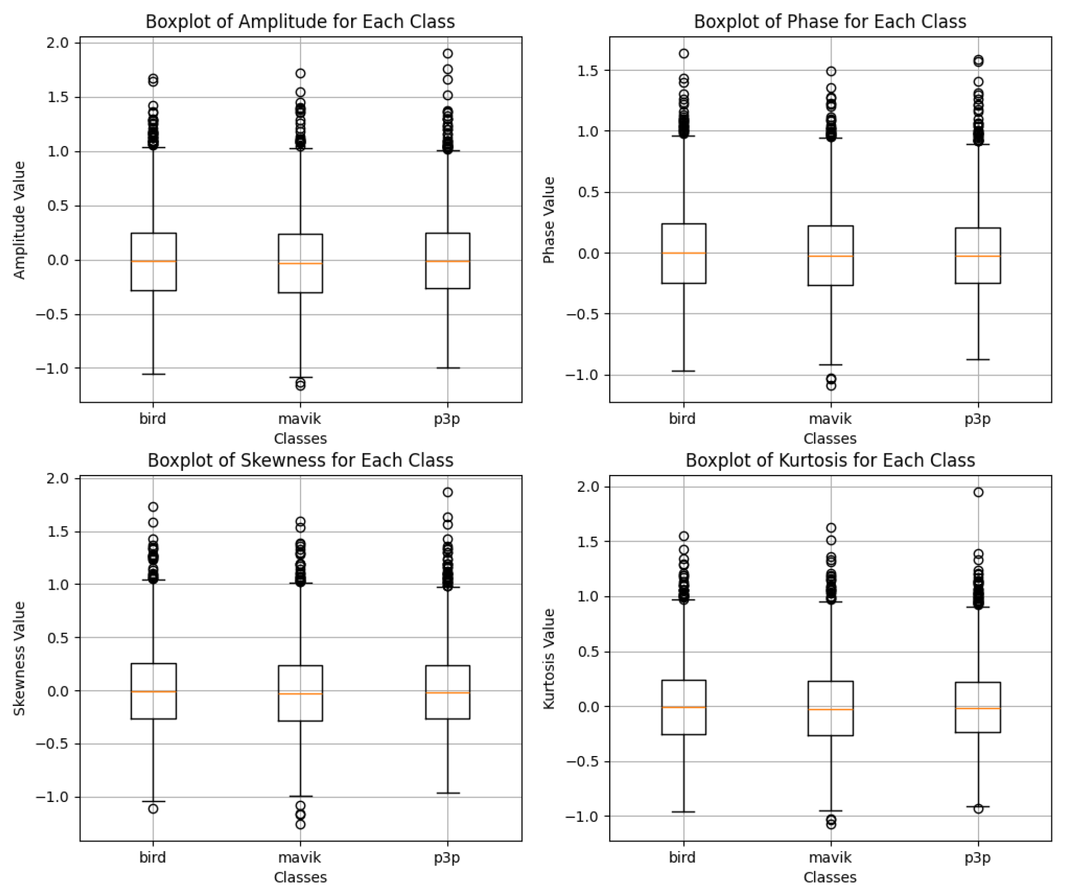
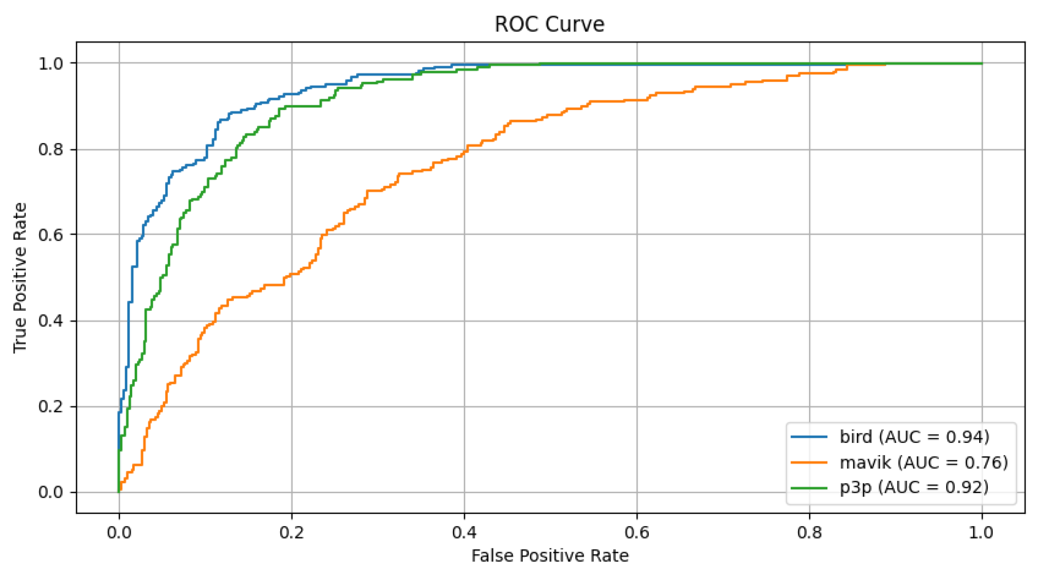
For Pareto noise, which was previously our critical case, even with the Transformer, there are a couple of more visible outliers at least in the amplitude and kurtosis measures, but the main bulk of distribution, as represented in the box-plot (Figure 15) through the interquartile ranges and medians, remains very similar across classes. Pareto noise has slightly positively skewed distribution characteristics as compared to impulsive noise, but such a difference does not tend to produce anything remarkably dissimilar lead in overall similarity between classes. Yet, it does cater in causing difficulties in classification which follows adequately with the noted fact that accuracy of multimodal transformer is lesser in this scenario, as can be seen in Figure 16.
Based on the graphs analyzed in Figure Figure 17, the box plots for impulsive noise reveal similar distributions among the classes "bird", "mavik" and "p3p" in all the evaluated metrics (amplitude, phase, skewness and kurtosis). There are no significant differences in central values, dispersion, or presence of outliers indicating any substantial changes caused by impulsive noise. This patchiness can be interpreted as not strong enough with respect to the effect of impulsive noise on the data–at least in reference to those metrics-to distinguish patterns overwhelmingly classifying the data into groups (Figure 18).
Figure 17.
Data distribution for the classification of bird, mavic drone, and P3P drone considering impulsive noise for classification with Multimodal Transformer.
Figure 17.
Data distribution for the classification of bird, mavic drone, and P3P drone considering impulsive noise for classification with Multimodal Transformer.
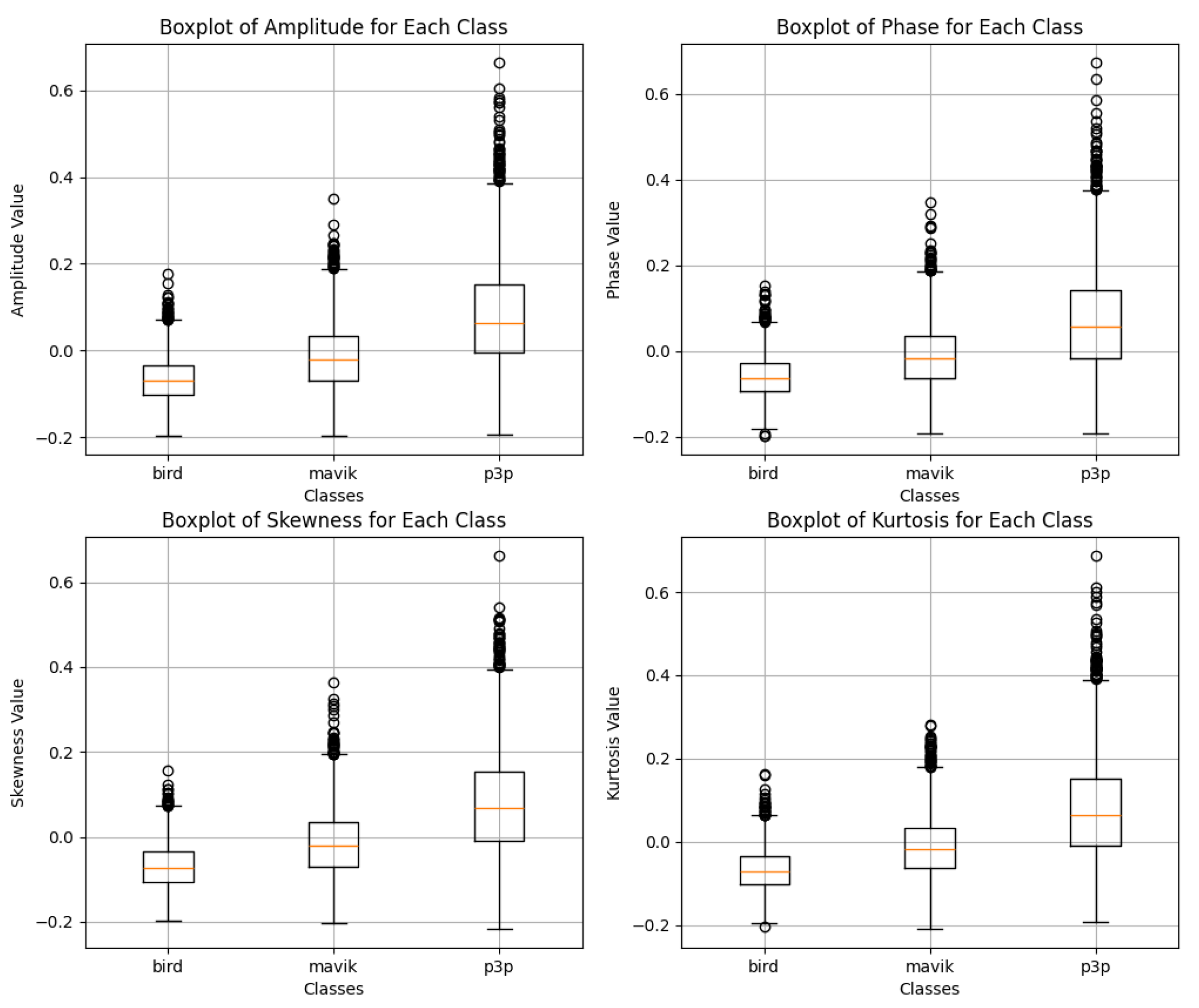
Figure 18.
ROC curves for the classification of bird, mavic drone, and P3P drone considering impulsive noise with Multimodal Transformer.
Figure 18.
ROC curves for the classification of bird, mavic drone, and P3P drone considering impulsive noise with Multimodal Transformer.
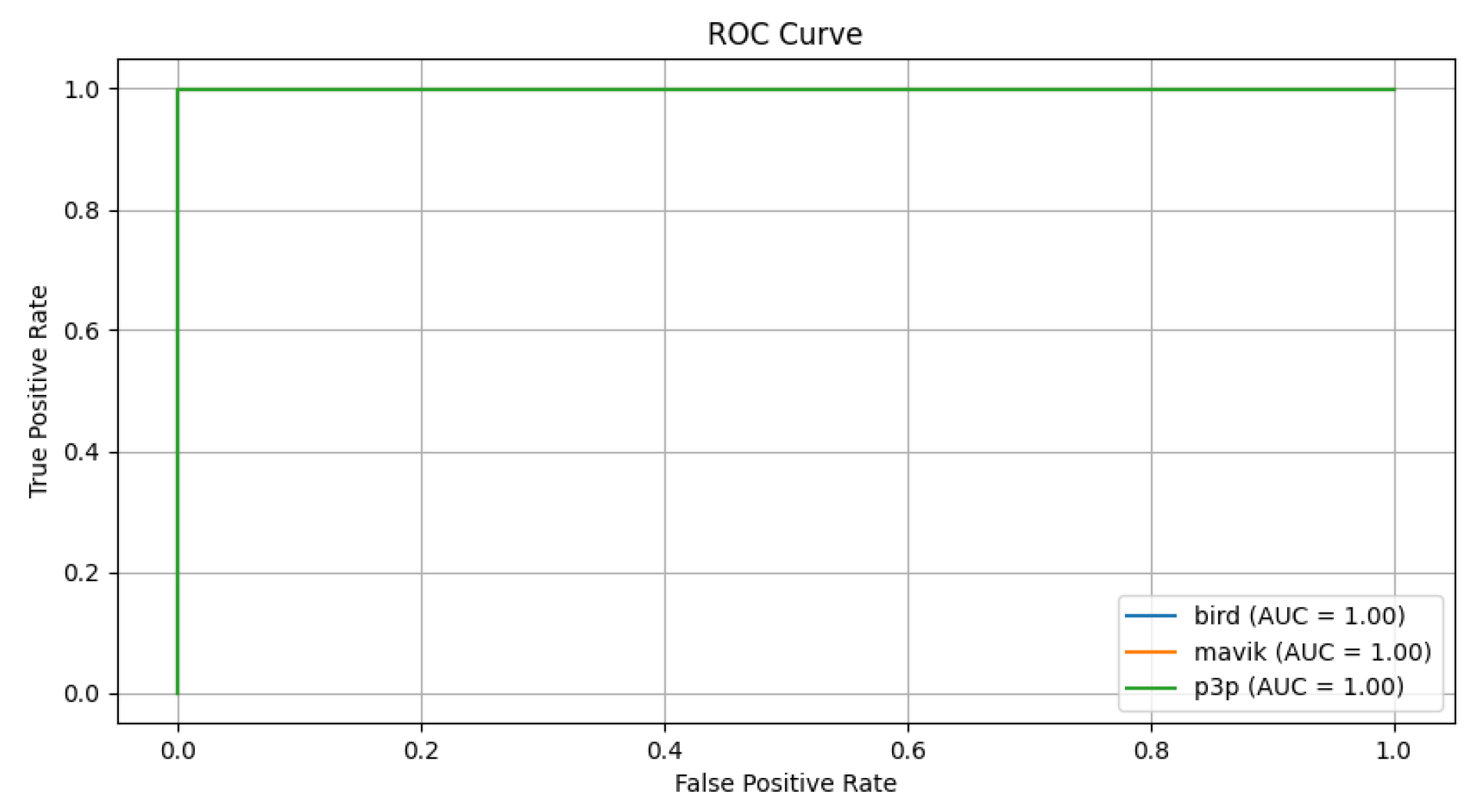
Figure 19.
ROC curves for the classification of bird, mavic drone, and P3P drone considering impulsive noise with Multimodal Transformer.
Figure 19.
ROC curves for the classification of bird, mavic drone, and P3P drone considering impulsive noise with Multimodal Transformer.
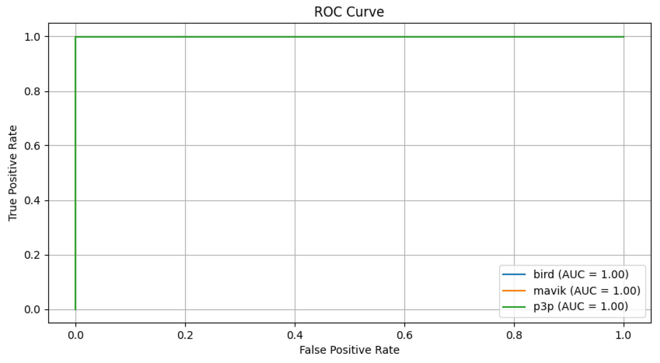
Figure 20.
Data distribution for the classification of bird, mavic drone, and P3P drone considering impulsive noise for classification with Multimodal Transformer.
Figure 20.
Data distribution for the classification of bird, mavic drone, and P3P drone considering impulsive noise for classification with Multimodal Transformer.
5. Discussion
The excellent performance exhibited by the Multimodal Transformer model in distinguishing drone and bird classes shows that there are several factors that play a key role in its robustness against noise interference. One important attribute is the use of attention mechanisms as these allow the model to refer the input data only to the relevant parts reducing the effect of impact from noise. Features such as amplitude, phase, skewness of amplitude as well as kurtosis of amplitude are critical in the retention of significant signal characteristics. These features still remained informative despite the introduction of white noise, Pareto noise, impulsive noise or multipath interference and made it possible for the Transformer to achieve near perfect classification.
The architecture of Transformer is structurally built to capture very complex non-linear relationships between features that may not be captured by other models. Unlike traditional methods that may be considered biased towards simple or localized patterns, mechanisms of Transformer tend to weigh the input features on the entire set. This flexibility allows the system to pick up those very minor features embedded in the data, which is important for accurate classification even under noise.
In addition, there is a self-embedded feature of the model of extraction and ranking of critical information from variously input characteristics so that the irrelevant noise does not overpower the important parts of the signal. This then depicts the noise resilience of the Transformer, showing its propensity for intricate feature extraction and analytical interpretation, which shall be useful in classifying signals from radar within the difficult environments encountered in real life.
6. Conclusions
This work was able to demonstrate the Multimodal Transformer model performing exceptionally in the classification of drone and bird signals in the presence of different types of noise such as white noise, Pareto noise, impulsive noise, and multipath interference without really degrading the accuracy much. This superiority regarding the performance of the model occurs mainly because the attention mechanisms are effectively used to focus on the most relevant features in data which gets heavily manipulated by noise. The features that were considered were amplitude, phase, skewness of amplitude, and kurtosis of amplitude and were used to thoroughly cover the characteristics of the signals which the Transformer takes to class description.
Noise is, of course, a big problem, yet the very high AUCs of all the noise types demonstrate how robust the Multimodal Transformer model is in handling complex and noisy input data. However, the model’s additional capability to include both statistical ones, namely skewness and kurtosis, and physical ones, that is amplitude and phase, is expected to contribute to capturing very subtle but meaningful patterns and generalizing the beyond what is necessary. The importance of this trait becomes even more important in real-world practical use cases where radar and sensor data are invariably noisy due to many sources, just as in the cases of aerial object detection.
From these findings, it can be inferred that most probably the architecture of the Transformer can fulfill the need for noisy radar signal classification. Further research could test more feature combinations in the model or optimized further to face other operational issues. The results pave a smooth path toward improving the reliability and efficiency of automatic drone detection systems in environments of different and very dense noise conditions.
Abbreviations
The following abbreviations are used in this manuscript:
| DJI | Dà-Jiāng Innovations Science and Technology Co., Ltd. |
| Conv1D | One-dimensional Convolutional Neural Network |
| LSTM | Long Short-Term Memory |
| GRU | Gated Recurrent Unit |
| CNN | Convolutional Neural Network |
| UAV | Unmanned Aerial Vehicle |
| C-UAV | Counter-Unmanned Aerial Vehicle |
| MLLM | Multimodal Large Language Model |
| mmWave | Millimeter Wave |
| CVMD | Complex-Valued Micro-Doppler |
| SVD | Singular Value Decomposition |
| ECSB | Echo Cancellation for Signal-Based Systems |
| FMCW | Frequency-Modulated Continuous Wave |
| RCS | Radar Cross Section |
References
- Clark, B. United States. In Calcagno, E.; Marrone, A., Eds. Above and Beyond: State of the Art of Uncrewed Combat Aerial Systems and Future Perspectives; Istituto Affari Internazionali (IAI): City, Country, 2023; pp. 31–37. Available online: http://www.jstor.org/stable/resrep55314.6 (accessed on Day Month Year).
- Pettyjohn, S. Types of Drones. In Evolution Not Revolution: Drone Warfare in Russia’s 2022 Invasion of Ukraine; Center for a New American Security: Washington, DC, USA, 2024; pp. 16–37. Available online: http://www.jstor.org/stable/resrep57900.7 (accessed on Day Month Year).
- Mohammed, A. B.; Fourati, L. C.; Fakhrudeen, A. M. Comprehensive systematic review of intelligent approaches in UAV-based intrusion detection, blockchain, and network security. Computer Networks 2023, 110140. [Google Scholar] [CrossRef]
- Seidaliyeva, U.; Omarbekova, A.; Abdrayev, S.; Mukhamezhanov, Y.; Kassenov, K.; Oyewole, O.; Koziel, S. Advances and challenges in drone detection and classification techniques: A state-of-the-art review. Sensors 2023, 24, 125. [Google Scholar] [CrossRef] [PubMed]
- Solaiman, S.; Alsuwat, E.; Alharthi, R. Simultaneous Tracking and Recognizing Drone Targets with Millimeter-Wave Radar and Convolutional Neural Network. Appl. Syst. Innov. 2023, 6, 68. [Google Scholar] [CrossRef]
- Dumitrescu, C.; Pleşu, G.; Băbuţ, M.; Dobrinoiu, C.; Dospinescu, A.; Botezatu, N. Development of an acoustic system for UAV detection. Sensors 2020, 20, 4870. [Google Scholar] [CrossRef] [PubMed]
- Song, C.; Li, H. An Acoustic Array Sensor Signal Recognition Algorithm for Low-Altitude Targets Using Multiple Five-Element Acoustic Positioning Systems with VMD. Appl. Sci. 2024, 14, 1075. [Google Scholar] [CrossRef]
- Li, D.; Li, Z.; He, S.; Du, W.; Wei, Z. Multi-source threatening event recognition scheme targeting drone intrusion in the fiber optic DAS system. IEEE Sens. J. 2024. [Google Scholar]
- Chen, T.; Yu, J.; Yang, Z. Research on a Sound Source Localization Method for UAV Detection Based on Improved Empirical Mode Decomposition. Sensors 2024, 24, 2701. [Google Scholar] [CrossRef] [PubMed]
- Tejera-Berengue, D.; Zhu-Zhou, F.; Utrilla-Manso, M.; Gil-Pita, R.; Rosa-Zurera, M. Acoustic-Based Detection of UAVs Using Machine Learning: Analysis of Distance and Environmental Effects. In Proceedings of the 2023 IEEE Sensors Applications Symposium (SAS), Ottawa, ON, Canada, 2023; pp. 1–6. [Google Scholar] [CrossRef]
- Utebayeva, D.; Ilipbayeva, L.; Matson, E.T. Practical study of recurrent neural networks for efficient real-time drone sound detection: A review. Drones 2023, 7, 26. [Google Scholar] [CrossRef]
- He, J.; Fakhreddine, A.; Alexandropoulos, G.C. RIS-Augmented Millimeter-Wave MIMO Systems for Passive Drone Detection. arXiv 2024, arXiv:2402.07259. [Google Scholar]
- Zhai, X.; Zhou, Y.; Zhang, L.; Wu, Q.; Gao, W. YOLO-Drone: an optimized YOLOv8 network for tiny UAV object detection. Electronics 2023, 12, 3664. [Google Scholar] [CrossRef]
- Sen, C.; Singh, P.; Gupta, K.; Jain, A. K.; Jain, A.; Jain, A. UAV Based YOLOV-8 Optimization Technique to Detect the Small Size and High Speed Drone in Different Light Conditions. In Proceedings of the 2024 2nd International Conference on Disruptive Technologies (ICDT); IEEE, 2024; pp. 1057–1061. [Google Scholar]
- Cheng, Q.; Li, X.; Zhu, B.; Shi, Y.; Xie, B. Drone detection method based on MobileViT and CA-PANet. Electronics 2023, 12, 223. [Google Scholar] [CrossRef]
- Muhamad Zamri, F.N.; Gunawan, T.S.; Yusoff, S.H.; Alzahrani, A.A.; Bramantoro, A.; Kartiwi, M. Enhanced Small Drone Detection Using Optimized YOLOv8 With Attention Mechanisms. IEEE Access 2024, 12, 90629–90643. [Google Scholar] [CrossRef]
- Zeng, Y.; Wang, G.; Hong, T.; Wu, H.; Yao, R.; Song, C.; Zou, X. UAVData: A Dataset for Unmanned Aerial Vehicle Detection. Soft Comput. 2021, 25, 5385–5393. [Google Scholar] [CrossRef]
- El-Latif, E.I.A. Detection and identification of drones using long short-term memory and Bayesian optimization. Multimed. Tools Appl. 2024. [Google Scholar] [CrossRef]
- Xiao, J.; Pisutsin, P.; Tsao, C. W.; Feroskhan, M. Clustering-based Learning for UAV Tracking and Pose Estimation. arXiv preprint 2024, arXiv:2405.16867. [Google Scholar]
- Johnstone, C. B.; Cook, C. R.; Aldisert, A.; Klaas, L.; Michienzi, C.; Rubinstein, G.; Sanders, G.; Szechenyi, N. Case Study Two: Electro-Optical Sensors. In Building a Mutually Complementary Supply Chain between Japan and the United States: Pathways to Deepening Japan-U.S. Defense Equipment and Technology Cooperation; Center for Strategic and International Studies (CSIS): City, Country, 2024; pp. 16–20. Available online: http://www.jstor.org/stable/resrep62403.6 (accessed on Day Month Year).
- Yang, D.; Xie, X.; Zhang, Y.; Li, D.; Liu, S. A multi-rotor drone micro-motion parameter estimation method based on CVMD and SVD. Remote Sens. 2022, 14, 3326. [Google Scholar] [CrossRef]
- Hanif, A.; Ahmad, F.; Zhang, G.; Wang, X. Micro-Doppler based target recognition with radars: A review. IEEE Sens. J. 2022, 22, 2948–2961. [Google Scholar] [CrossRef]
- Soumya, A.; Mohan, C. K.; Cenkeramaddi, L. R. Recent advances in mmWave-radar-based sensing, its applications, and machine learning techniques: A review. Sensors 2023, 23, 8901. [Google Scholar] [CrossRef] [PubMed]
- Kumawat, H.C.; Chakraborty, M.; Raj, A.A.B. DIAT-RadSATNet—A novel lightweight DCNN architecture for micro-Doppler-based small unmanned aerial vehicle (SUAV) targets’ detection and classification. IEEE Trans. Instrum. Meas. 2022, 71, 1–11. [Google Scholar] [CrossRef]
- Kumawat, H.C.; Chakraborty, M.; Arockia Bazil Raj, A.; Dhavale, S.V. DIAT-µSAT: Micro-Doppler Signature Dataset of Small Unmanned Aerial Vehicle (SUAV). IEEE Dataport 2022. [Google Scholar] [CrossRef]
- Texas Instruments. The fundamentals of millimeter wave radar sensors. Available online: https://www.ti.com/lit/wp/spry325/spry325.pdf (accessed on 10 September 2024).
- Lu, G.; Bu, Y. Mini-UAV Movement Classification Based on Sparse Decomposition of Micro-Doppler Signature. IEEE Geosci. Remote Sens. Lett. 2024. [Google Scholar] [CrossRef]
- Kang, S.; Forsten, H.; Semkin, V.; Rangan, S. Millimeter Wave 60 GHz Radar Measurements: UAS and Birds. IEEE Dataport 2024. [Google Scholar]
- Narayanan, R.M.; Tsang, B.; Bharadwaj, R. Classification and Discrimination of Birds and Small Drones Using Radar Micro-Doppler Spectrogram Images. Signals 2023, 4, 337–358. [Google Scholar] [CrossRef]
- Yan, J.; Hu, H.; Gong, J.; Kong, D.; Li, D. Exploring Radar Micro-Doppler Signatures for Recognition of Drone Types. Drones 2023, 7, 280. [Google Scholar] [CrossRef]
- Fan, S.; Wu, Z.; Xu, W.; Zhu, J.; Tu, G. Micro-Doppler Signature Detection and Recognition of UAVs Based on OMP Algorithm. Sensors 2023, 23, 7922. [Google Scholar] [CrossRef] [PubMed]
- Ye, J.; Gu, F.; Wu, H.; Han, X.; Yuan, X. A new frequency hopping signal detection of civil UAV based on improved k-means clustering algorithm. IEEE Access 2021, 9, 53190–53204. [Google Scholar] [CrossRef]
- Xu, C.; Tang, S.; Zhou, H.; Zhao, J.; Wang, X. Adaptive RF fingerprint decomposition in micro UAV detection based on machine learning. In Proceedings of the ICASSP 2021-2021 IEEE International Conference on Acoustics, Speech and Signal Processing (ICASSP), Toronto, Canada, 6–11 June 2021. [Google Scholar]
- Inani, K. N.; Sangwan, K. S.; Dhiraj. Machine Learning based framework for Drone Detection and Identification using RF signals. In In Proceedings of the 2023 4th International Conference on Innovative Trends in Information Technology (ICITIIT), Kottayam, India; 2023; pp. 1–8. [Google Scholar] [CrossRef]
- Mandal, S.; Satija, U. Time–Frequency Multiscale Convolutional Neural Network for RF-Based Drone Detection and Identification. IEEE Sensors Letters 2023, 7, 1–4. [Google Scholar] [CrossRef]
- Garvanov, I.; Kanev, D.; Garvanova, M.; Ivanov, V. Drone Detection Approach Based on Radio Frequency Detector. In Proceedings of the 2023 International Conference Automatics and Informatics (ICAI), Varna, Bulgaria; 2023; pp. 230–234. [Google Scholar] [CrossRef]
- Xu, P.; Zhu, X.; Clifton, D. A. Multimodal learning with transformers: A survey. IEEE Trans. Pattern Anal. Mach. Intell. 2023, 45, 12113–12132. [Google Scholar] [CrossRef]
Figure 1.
White noise affects the signal uniformly, with moderate variability and considerable outliers.
Figure 1.
White noise affects the signal uniformly, with moderate variability and considerable outliers.

Figure 2.
The heavy-tailed error distribution from Pareto noise, with noticeable spikes and outliers.
Figure 2.
The heavy-tailed error distribution from Pareto noise, with noticeable spikes and outliers.
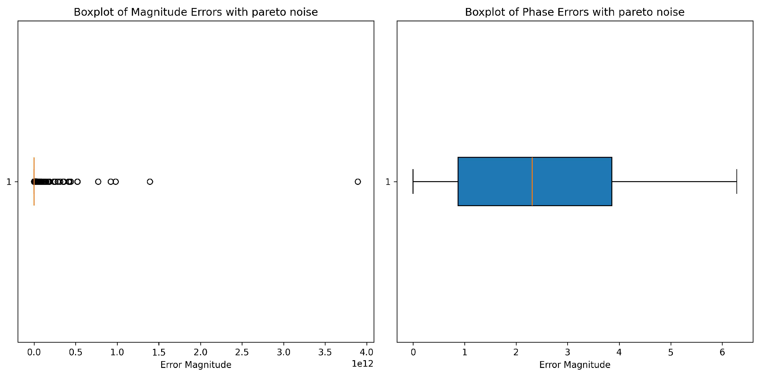
Figure 3.
The effects of impulsive noise on amplitude and phase errors.
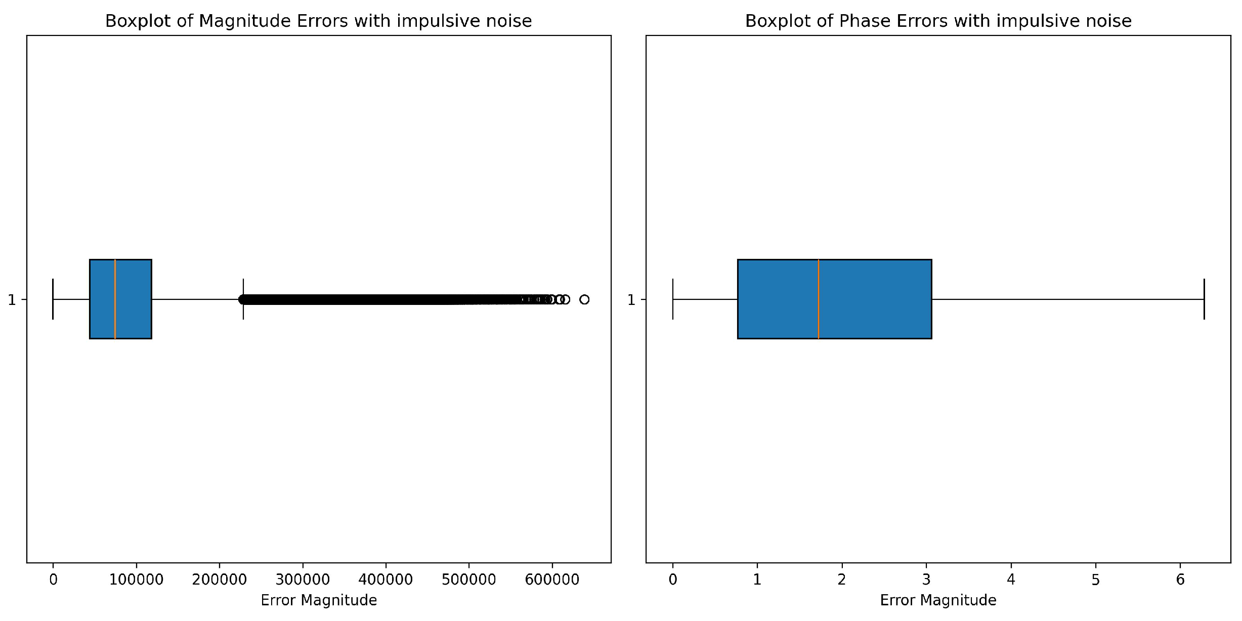
Figure 4.
Multipath interference introduces strong amplitude fluctuations.
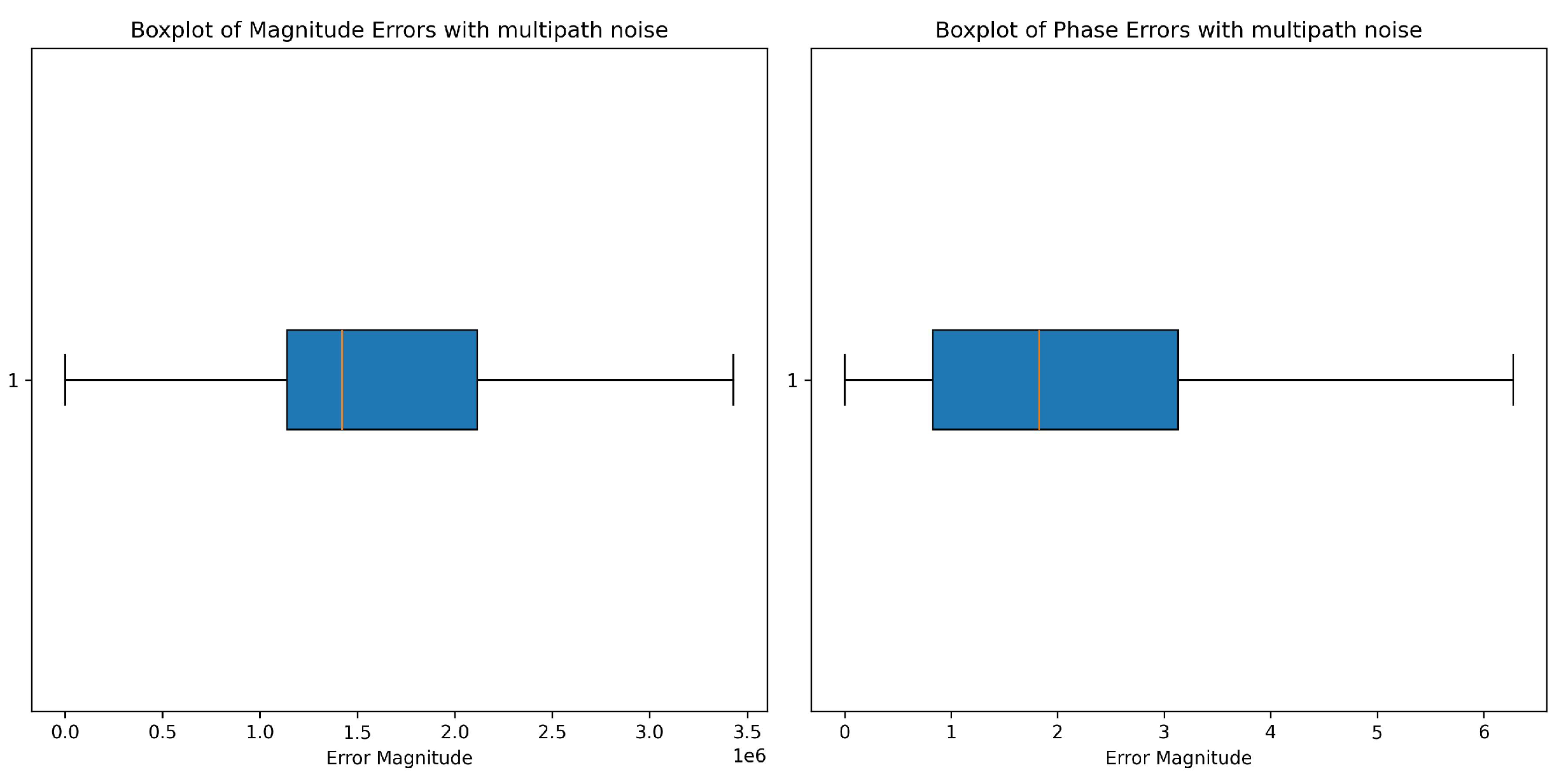
Figure 5.
Data distribution for the classification of bird, mavic drone, and P3P drone considering white noise conditions.
Figure 5.
Data distribution for the classification of bird, mavic drone, and P3P drone considering white noise conditions.
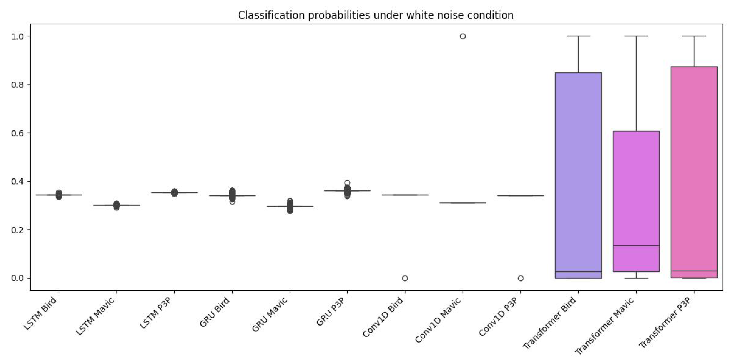
Figure 6.
ROC plots for the classification algorithms LSTM, GRU, CONV1D, and Transformer under scenarios with white noise.
Figure 6.
ROC plots for the classification algorithms LSTM, GRU, CONV1D, and Transformer under scenarios with white noise.
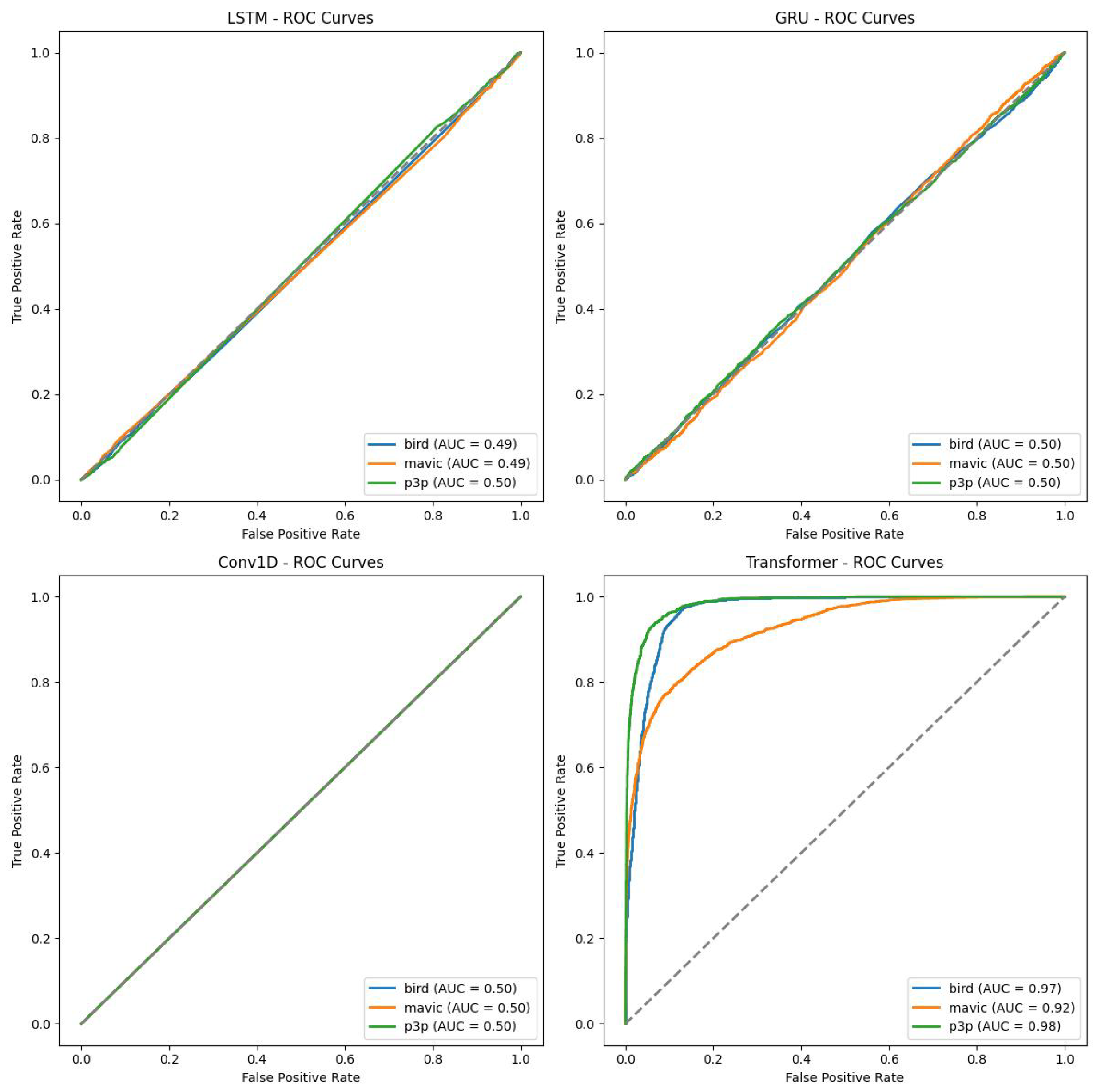
Figure 7.
Data distribution for the classification of bird, mavic drone, and P3P drone considering Pareto noise.
Figure 7.
Data distribution for the classification of bird, mavic drone, and P3P drone considering Pareto noise.
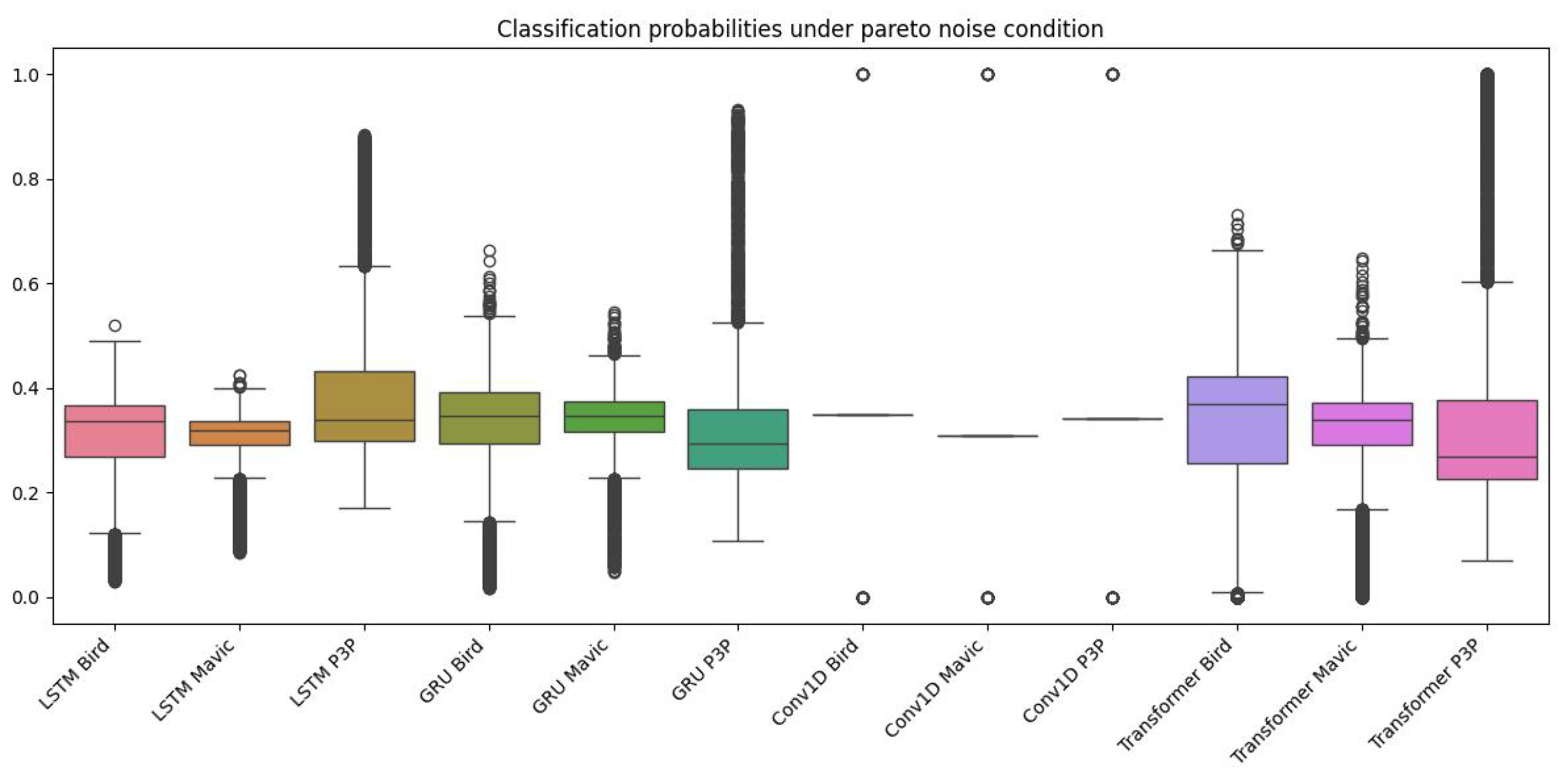
Figure 8.
ROC curves for LSTM, GRU, CONV1D, and Transformer under Pareto noise conditions.
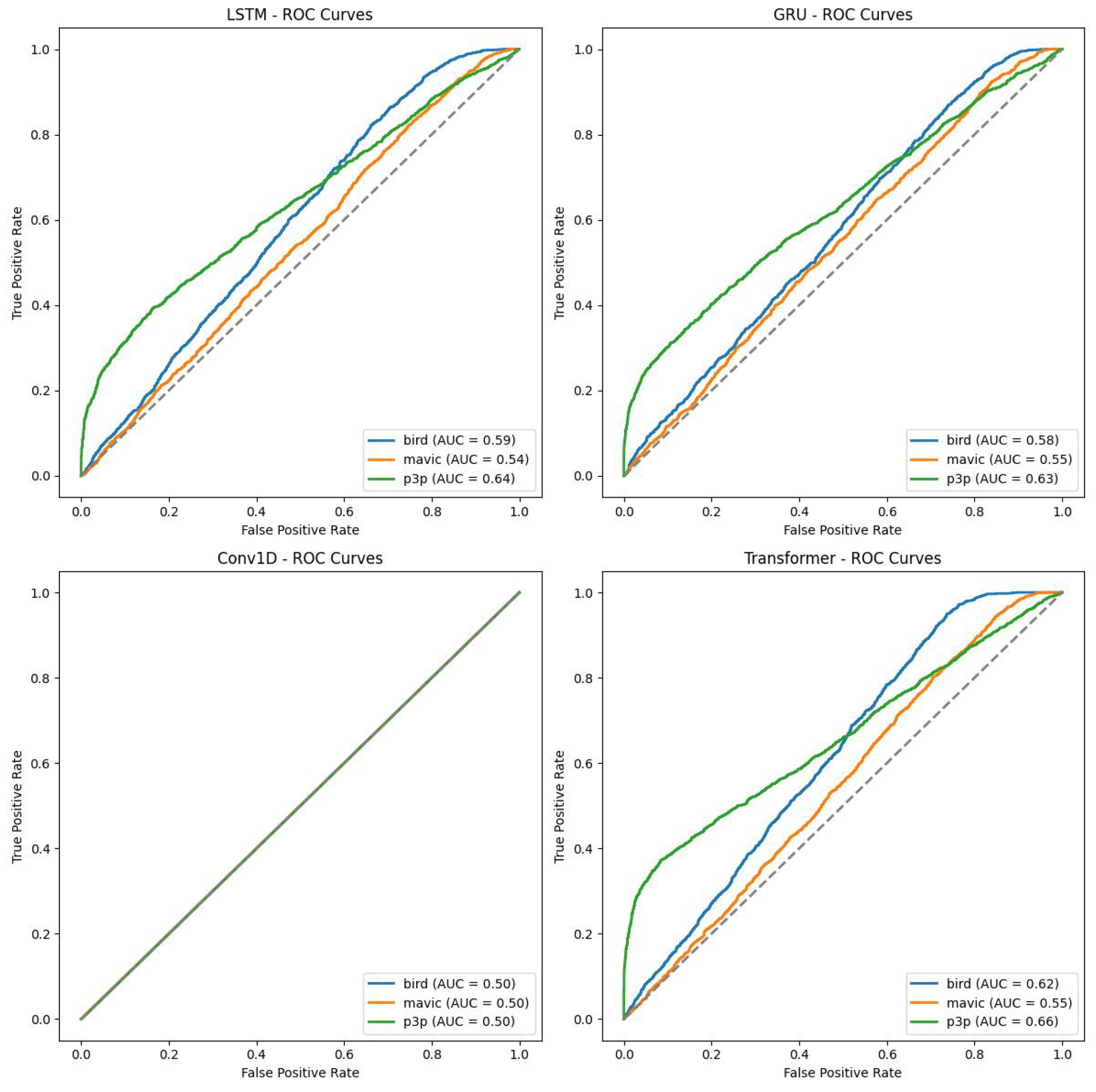
Figure 9.
Data distribution for the algorithms LSTM, GRU, CONV1D, and Transformer under impulsive noise conditions.
Figure 9.
Data distribution for the algorithms LSTM, GRU, CONV1D, and Transformer under impulsive noise conditions.
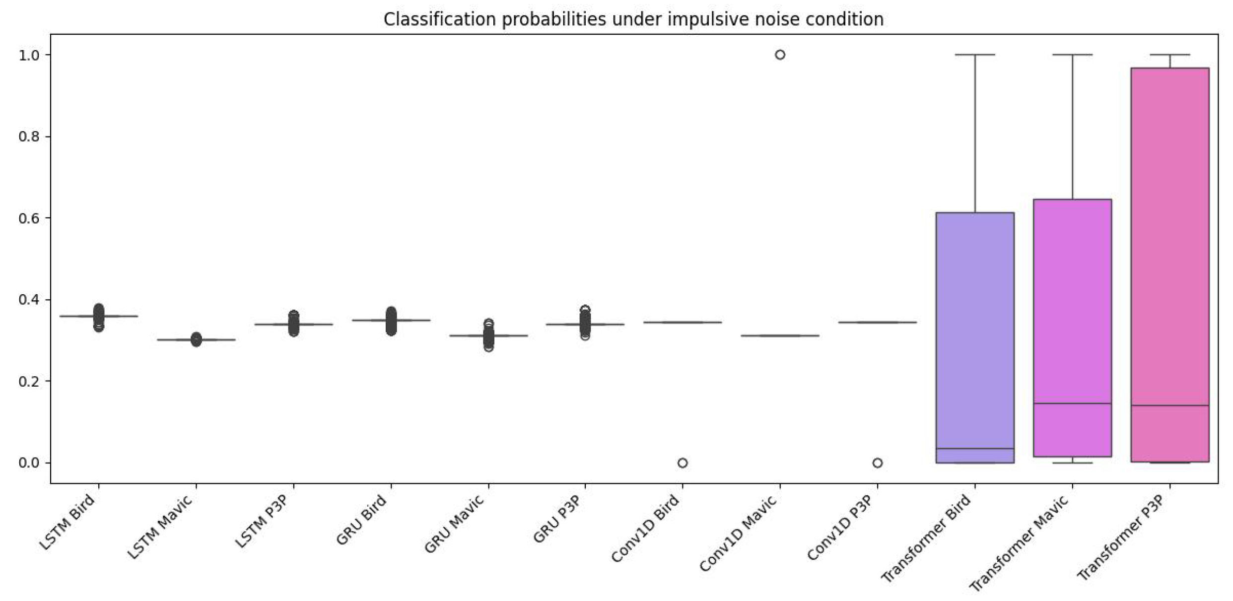
Figure 10.
ROC curves for LSTM, GRU, CONV1D, and Transformer under impulsive noise conditions.
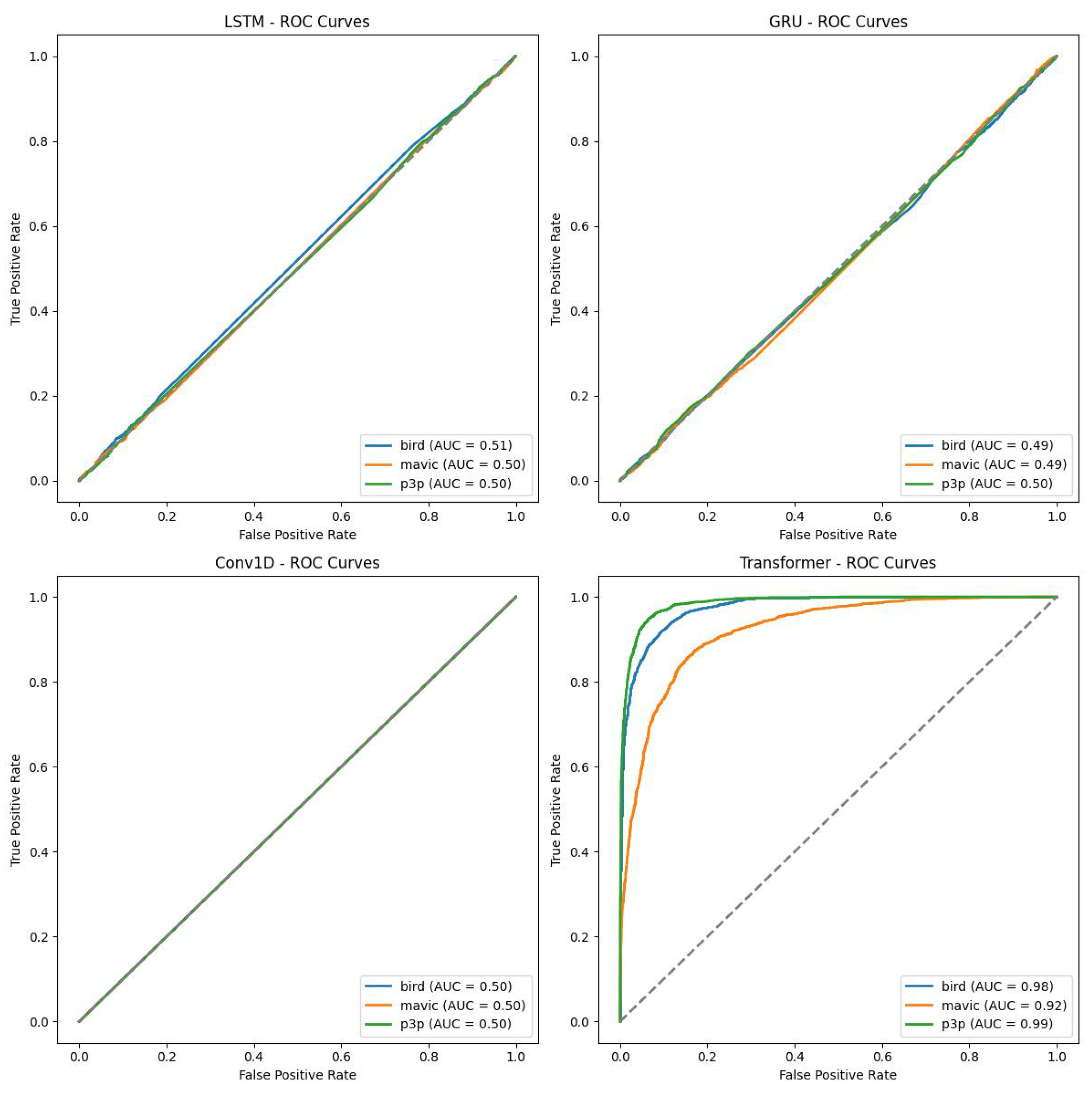
Figure 11.
Data distribution for the algorithms LSTM, GRU, CONV1D, and Transformer under multipath interference.
Figure 11.
Data distribution for the algorithms LSTM, GRU, CONV1D, and Transformer under multipath interference.
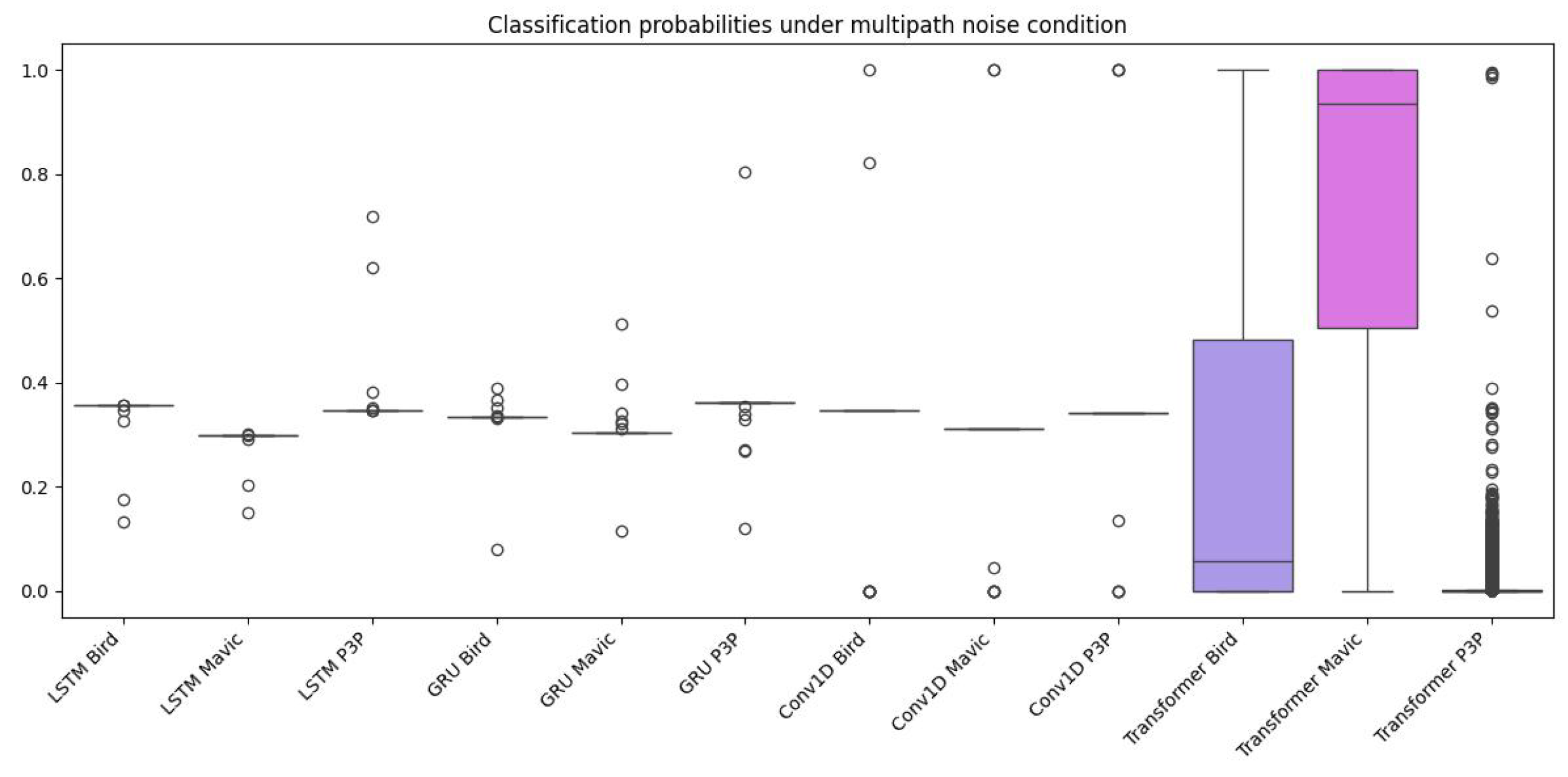
Figure 12.
ROC curves for LSTM, GRU, CONV1D, and Transformer under multipath conditions.
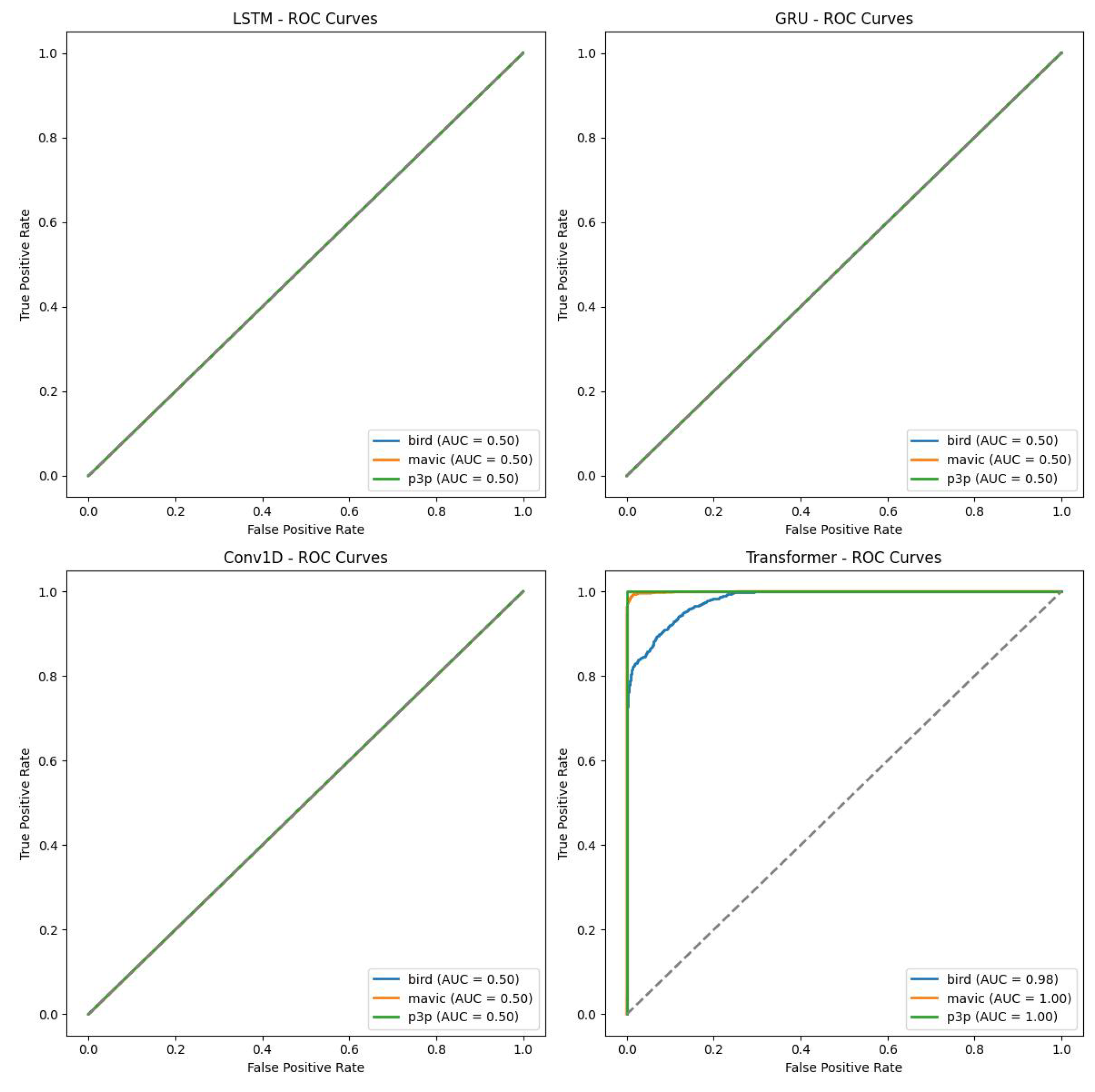
Figure 13.
Data distribution for the classification of bird, mavic drone, and P3P drone considering white noise for classification with Multimodal Transformer.
Figure 13.
Data distribution for the classification of bird, mavic drone, and P3P drone considering white noise for classification with Multimodal Transformer.
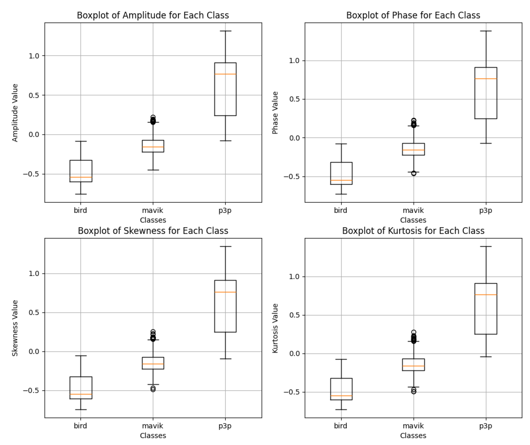
Figure 14.
ROC curves for the classification of bird, mavic drone, and P3P drone considering white noise with Multimodal Transformer.
Figure 14.
ROC curves for the classification of bird, mavic drone, and P3P drone considering white noise with Multimodal Transformer.
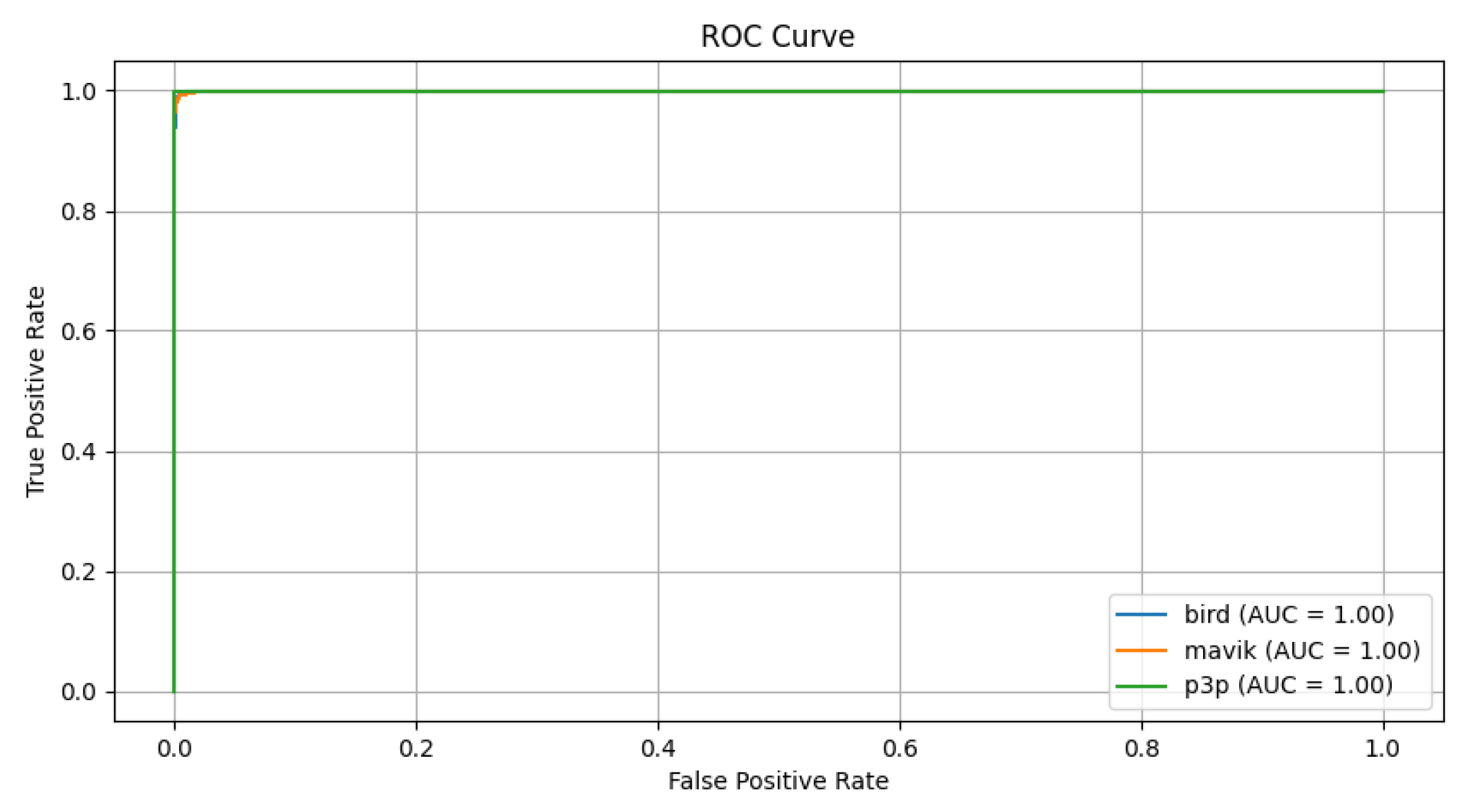
Figure 15.
Data distribution for the classification of bird, mavic drone, and P3P drone considering Pareto noise for classification with Multimodal Transformer.
Figure 15.
Data distribution for the classification of bird, mavic drone, and P3P drone considering Pareto noise for classification with Multimodal Transformer.
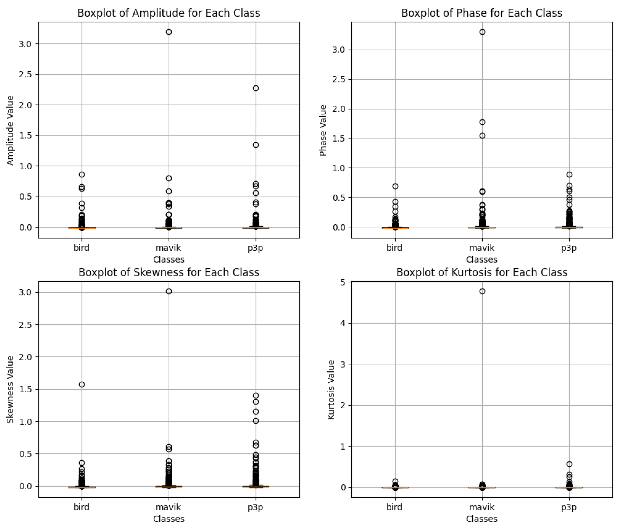
Figure 16.
ROC curves for the classification of bird, mavic drone, and P3P drone considering Pareto noise with Multimodal Transformer.
Figure 16.
ROC curves for the classification of bird, mavic drone, and P3P drone considering Pareto noise with Multimodal Transformer.
Disclaimer/Publisher’s Note: The statements, opinions and data contained in all publications are solely those of the individual author(s) and contributor(s) and not of MDPI and/or the editor(s). MDPI and/or the editor(s) disclaim responsibility for any injury to people or property resulting from any ideas, methods, instructions or products referred to in the content. |
© 2024 by the authors. Licensee MDPI, Basel, Switzerland. This article is an open access article distributed under the terms and conditions of the Creative Commons Attribution (CC BY) license (http://creativecommons.org/licenses/by/4.0/).
Copyright: This open access article is published under a Creative Commons CC BY 4.0 license, which permit the free download, distribution, and reuse, provided that the author and preprint are cited in any reuse.


