
Submitted:
31 July 2025
Posted:
01 August 2025
You are already at the latest version
Abstract
Coastal communities and marine ecosystems face increasing risks due to changing ocean conditions, yet effective wave monitoring remains limited in many low-resource regions. This study investigates the use of seismic data to predict significant wave height (SWH), offering a low-cost and scalable solution to support coastal conservation and safety. We developed a baseline machine learning (ML) model and improved it using a longest-stretch algorithm for seismic data selection and station-specific hyperparameter tuning. Models were trained and tested on consumer-grade hardware to ensure accessibility and availability. Applied to the Sicily-Malta region, the enhanced models achieved up to a 0.133 increase in R2 and a 0.026m reduction in mean absolute error compared to existing baselines. These results demonstrate that seismic signals, typically collected for geophysical purposes, can be repurposed to support ocean monitoring using accessible artificial intelligence (AI) tools. The approach may be integrated into conservation planning efforts such as early warning systems and ecosystem monitoring frameworks. Future work may focus on improving robustness in data-sparse areas through augmentation techniques and exploring broader applications of this method in marine and coastal sustainability contexts.
Keywords:
coastal conservation
; seismic data
; ocean monitoring
; wave prediction
; artificial intelligence
; low-resource technology
; marine sustainability
; environmental monitoring
1. Introduction
Marine and coastal ecosystems are central to the sustainability of over three billion people worldwide, impacting their livelihoods, food security, and safety [1]. These regions support rich biodiversity and serve as buffers against natural hazards, yet they are increasingly threatened by climate change, rising sea levels, and extreme weather events. Accurate and timely knowledge of sea conditions, particularly SWH, is essential for informed conservation planning, marine spatial governance, and coastal risk mitigation. However, real-time ocean monitoring systems remain limited, particularly in low-resource settings where high-cost instrumentation and data infrastructure are not viable.
Conventional wave monitoring approaches, such as ocean buoys and weather satellites face logistical, financial, and technical challenges. Devices deployed at sea are often dislodged and set adrift, contributing to marine pollution. This debris, including discarded mooring lines, poses a serious threat to marine life; for example, sea turtles can become entangled, leading to injury or death [2]. Moreover, buoys are susceptible to damage from marine life, vessel collisions, and extreme weather, while satellite-based methods are constrained by fuel limitations and the growing issue of orbital debris, or `space junk’. These limitations hinder the development of sustainable and scalable ocean observation systems.
Ocean waves, predominantly driven by weather systems, can induce ground motion when they reach coastlines. These motions generate continuous low-frequency seismic signals, known as microseisms. Despite being historically considered noise, microseisms are now a valuable data source for studying oceanographic and geophysical processes [4,5]. Microseisms mainly occur in two frequency bands: primary (0.05–0.1 Hz) and secondary (0.1–0.5 Hz) [6,7]. The lower-frequency microseisms result from direct pressure on the ocean floor, while secondary ones stem from wave-wave interactions. These signals correlate with ocean wave energy, typically measured through SWH, derived from spectral wave data [8].
Recent research has explored alternative proxies for wave monitoring including seismic signals generated by ocean wave activity [6,7,9,10]. These signals, particularly microseisms, are detectable by seismometers located on land. To this end, they offer a low-cost, low-maintenance solution for continuous data acquisition. While studies have confirmed a correlation between microseismic amplitude and SWH [6], few have systematically applied AI to model this relationship in a way that supports environmental monitoring and conservation outcomes. Moreover, existing AI-based approaches often rely on large, spatially diverse datasets that overlook local variability in seismic–oceanic interactions. Many also depend on extensive interpolation to address data gaps that sometimes span hundreds of days. The impact of such extensive gaps on model accuracy and ecological relevance remain unclear.
In response to these limitations, this study investigates whether seismic signals can reliably predict SWH using accessible, regionally tuned AI models. Focusing on the Sicily–Malta region, we developed a reproducible baseline and improved upon it using efficient algorithms and station-specific tuning strategies. Models were trained on consumer-grade hardware with minimal preprocessing, promoting equitable access to ocean monitoring tools. Our findings show that low-frequency seismic amplitude can serve as a dependable proxy for SWH, enabling the development of lightweight and cost-effective systems for real-time wave estimation. The study demonstrates the potential for scalable, AI-driven solutions in marine sensing, with implications for coastal conservation, risk assessment, and sustainable resource management.
1.1. Literature Review
This section will provide an overview of the current technologies used for estimating wave parameters, including both AI-based methods and other approaches. While surveying existing technologies for estimating wave parameters, areas for further improvement will also be identified.
1.1.1. Numerical Methods Approaches
Several traditional numerical approaches have been used to estimate wave parameters from seismic data, offering valuable insights and benchmarks. Ferretti et al. [6] investigated the relationship between the microseism and SWH during a major storm event in the Ligurian Sea. Their approach involved pre-processing seismic signals, converting them to the frequency domain using Fourier transforms, and establishing a statistical relationship between microseism power spectral density (PSD) and SWH. A Markov chain Monte Carlo (MCMC) method was used to estimate parameters in an empirical model. Their refined model achieved a high cross-correlation (93%) with observed wave heights, though errors up to 1.75m were noted in extreme cases. While not AI-based, their method demonstrates the feasibility of inferring wave parameters from land-based seismic data and offers valuable baseline metrics.
In a more recent study, Borzi et al. [7] examined seismic signatures during Medicane Helios, a 2023 Mediterranean cyclone. Using spectral and correlation analysis across over 100 seismic stations, they established links between microseism signal characteristics and wave field variations, supported by satellite and radar observations. Their spatial analysis confirmed that higher frequency seismic bands exhibited stronger correlations with SWH, consistent with Ferretti’s earlier findings.
These studies show that wave-seismic relationships can be reliably quantified using signal processing and statistical modelling. However, numerical methods can be complex, computationally intensive, and site-specific, motivating the exploration of more scalable, generalisable AI-based alternatives.
1.1.2. Artificial Intelligence Methods
Early research linking ocean microseisms to SWH laid the foundational groundwork for ML-based models in ocean state monitoring. Cannata et al. [9] were among the first to explore this relationship using a random forest (RF) regression model trained on the root mean square (RMS) amplitude of seismic signals, paired with hindcast SWH maps as targets. Their use of k-fold cross-validation ensured a measure of generalisability, and their results, particularly mean absolute error (MAE) values were as low as 0.1m along the Sicilian coast. This suggests strong local correlations between seismic activity and sea state.
Building upon this, Minio et al. [10] significantly extended the scope of AI-based ocean monitoring by training three supervised models: RF, k-nearest neighbours (KNN), and light gradient boosting (LGB). These models were trained on four years of seismic and oceanographic data (2018–2021). Unlike earlier efforts, their work aimed to construct a comprehensive and scalable solution, leveraging publicly available seismic data from the European Integrated Data Archive (EIDA) [11] and sea state data from Copernicus Marine Environment Monitoring Service (CMEMS) [12]. Notably, they incorporated an earthquake catalogue to exclude periods influenced by tectonic events, ensuring microseismic origins were predominantly oceanic.
Their seismic dataset comprised 14 coastal stations, each recording in three directions (vertical, north-south, east-west), resulting in a 588 features (14 stations × 14 frequency bands × 3 components). The region of interest is depicted in Figure 1. Pre-processing steps included linear interpolation for missing data, Box-Cox transformation for skewed distributions, and min-max normalisation, all aimed at enhancing model compatibility. While ensemble models such as RF and LGB are generally robust to skewed data, the application of the Box-Cox transformation may offer limited added value in this context and could introduce unnecessary computational overhead [13]. While the interpolation threshold applied by the authors helps maintain data continuity, literature suggests that gap-filling in seismic datasets is a complex task that often benefits from specialised methods [14,15].
Given the temporal autocorrelation in seismic signals, non-random splits can potentially lead to data leakage between training and testing sets. Minio et al. [10] addressed this by applying temporal chunking and random shuffling to reduce such risks. In this study, RF was found to perform the best (R = 0.89; MAE = 0.21 ± 0.23m). Such models are known to be resilient to noise, have a low sensitivity to hyperparameter tuning, and have the capability to model non-linear interactions. These likely contributed to its superior performance [17].
In a recent study, Baranbooei et al. [16] investigated the link between secondary microseisms and SWH near the Irish coast. Using data from a single buoy and five seismic stations, they applied a methodology similar to that of Minio et al. [10], including signal filtering, seismic event exclusion, and microseism amplitude computation.
One distinction in their approach was the reliance on a single buoy for sea state data. While this setup offers practical advantages, the spatial separation between the buoy and seismic stations may affect the reliability of the data, especially due to local variations in bathymetry and seismic wave propagation [18].
In particular, this study used approximately four years of valid data and trained artificial neural networks with five hidden layers, employing Bayesian regularisation to help mitigate overfitting. Two models, one using buoy-measured SWH and the other using wave model hindcast data, were assessed. Results indicated slightly better performance for the buoy-based model, especially for wave heights below 10m, though generalisation may still be influenced by region-specific geophysical factors.
Existing research has reported encouraging R² values above 0.8 and errors below 0.7m. However, some limitations remain. These include the absence of standardised benchmarks, varied preprocessing approaches, limited explanations for certain data transformations, and relatively little attention to spatial variability around seismic stations. Additionally, gap-filling methods are not always clearly described, and AI-based approaches, while promising, are still in early stages of development and assessment. These observations suggest an opportunity to further strengthen the field through more consistent methodologies and comprehensive evaluation frameworks.
1.2. Aims and Objectives
The aim of this study is to investigate the relationship between lower-frequency seismic amplitude and SWH, with a particular focus on the coastal regions of Sicily and Malta. The central objective is to establish a foundational baseline for future research in this domain. This study presents a baseline based on the work of Minio et al. [10], against which the performance of a set of models with an improved methodology is compared, offering evidence that complexity does not always equate to performance in this context, through a diverse set of evaluation metrics. Pipeline efficiency was improved through methodological clarity and the use of minimal synthetic data, foregoing more elaborate gap-filling techniques in favour of practical simplicity. Only seismic stations with sufficient data coverage – at least one full year of data – were included, ensuring the models were trained on data that captures seasonal variability. The following objectives have been addressed:
- Recreate and evaluate baseline models to establish the relationship between seismic RMS amplitude and SWH, using comprehensive evaluation metrics for fair comparison.
- Develop a cost-effective modelling approach, deployable on consumer-grade hardware, promoting accessibility in resource-constrained settings and supporting ethical AI practices.
- Design an efficient and deployable data pipeline that minimises preprocessing to ensure practical real-time inference with low system complexity.
- Apply location-specific hyperparameter tuning to optimise model performance across varying environmental and geographical conditions.
- Prioritise high-integrity, real-world data over interpolated or gap-filled datasets to improve model reliability and generalisability.
1.3. Contributions
This study contributes a reproducible baseline for predicting wave height from seismic data, supporting future research and applications. It shows that effective models can be trained on consumer-grade hardware, aiding deployment in low-resource settings. A novel algorithm selects long continuous data stretches, improving model reliability. Tailored tuning led to an improvement of up to 0.2566 in R² over baseline RF models. Analysis of certain stations highlighted data issues impacting performance, and the study highlights a dataset bias against extreme sea conditions, suggesting future improvements in data coverage.
2. Materials and Methods
Similarly to what was done by Minio et al. [10], seismic and sea state data from January 2018 to December 2021 were collected from the European Integrated Data Archive (EIDA) Seismic Network `IV’ [11] and the Copernicus Marine Environment Monitoring Service (CMEMS) MEDSEA_MULTIYEAR_WAV_006_012 [12], respectively. Additional seismic records for Malta’s WDD and MSDA stations obtained via the University of Malta. These Maltese stations were included to extend the geographical scope and contextual relevance of the study. Seismic data was sourced through the INGV network on EIDA [11], while sea state data came from the CMEMS [12]. Fourteen seismic stations in total were considered, spanning Sicily, Pantelleria, and Malta. The region of interest is depicted in Figure 2.
Preprocessing began with detrending each seismic signal via mean and linear trend removal, followed by bandpass filtering into 13 frequency bands based on Minio et al.’s implementation. The signals were scaled by station sensitivity and converted to hourly RMS using a more computationally efficient sliding window method in NumPy1, replacing the original ObsPy-based approach2. Sea state data were also optimised by expanding the region of interest, ensuring no relevant oceanic grid points were missed, particularly near Malta.
To avoid the information loss of using distant and poorly correlated sea state data, each seismic station was paired with its five nearest sea grid points. This pairing was established using distance calculations within a narrow radius of each station. To identify the longest continuous stretch of data for each station, a dynamic data selection algorithm was developed. The gap tolerance was incrementally adjusted to balance data continuity with informational value. Ultimately, gaps of up to eight hours were interpolated, enabling seven stations to meet the one-year data threshold.
This preprocessing strategy ensured a more spatially precise and computationally efficient dataset. As a result, seven stations (AIO, CAVT, CSLB, HAGA, MSDA, MUCR, and WDD, labelled in Figure 2), were retained for modelling, each with over a year of high-quality, minimally interpolated data. This approach improved upon the original study by enhancing both the geographical granularity and robustness of the input data.
2.1. Exploratory Data Analysis
This research explores how SWH can be inferred from coastal seismic signals more reliably using AI, based on the physical coupling between ocean waves and the Earth’s crust. Analysis began by comparing seismic stations to nearby sea state grid cells. While the stations in Malta showed strong correlations, others like HAGA, despite being closest to the coast, did not outperform more distant sites like MUCR, indicating that proximity alone does not determine predictive strength.
Temporal and statistical analyses followed. Spearman correlation peaked in the 0.2-0.5Hz bands, consistent with known ocean microseism activity. Autocorrelation showed faster decay at lower frequencies, suggesting sensitivity to sea state changes, while higher frequencies reflected more persistent signals which were likely anthropogenic. Seismic RMS distributions were skewed toward zero, supporting the use of ML models suited for non-normal data. These findings shaped the choice of training stations and informed feature engineering for modelling.
2.2. Model Selection
The model selection process was driven by both empirical observations and practical constraints. Exploratory analysis revealed high data skewness and low autocorrelation decay, especially in lower frequency bands, while higher frequencies were often contaminated by human activity. These properties made traditional linear or distance-based models unsuitable due to their sensitivity to skewed distributions and noise. Instead, tree-based models such as RF offered robustness to skewness, no reliance on distributional assumptions, and resilience against persistent anthropogenic signals. Furthermore, RF models are computationally efficient, requiring modest hardware for training and deployment, critical for real-world applicability. Given these advantages and the strong benchmark performance reported by Minio et al., this study adopted an RF regressor, using Scikit-learn (v1.5.2) as the core model3.
2.3. Creation of a Baseline
To evaluate model performance meaningfully, a reproducible baseline was established based on the methodology of Minio et al., with additional preprocessing steps for data refinement. The pipeline begins by extracting hourly seismic RMS from raw waveform data, then applying a noise threshold below which values were replaced with null values. Features with excessive null values (>5,000) were discarded, and remaining missing data were filled via linear interpolation. To address data skewness, features with skewness greater than 0.7 were transformed using the Box-Cox method. Additionally, data points affected by major seismic events (magnitude >5.5 in the Mediterranean or >7.0 globally) were removed, which required the integration of an earthquake catalogue4.
Target variables were constructed by identifying each station’s five nearest ocean grid cells and calculating both mean and median SWH values across them, resulting in seven targets per station. In total, each dataset comprised 39 input features (13 frequency bands × 3 channels). For training and testing, data were split into 40 non-consecutive chunks, with 70% randomly selected for training and 30% for testing. This chunking approach, adapted from Minio et al., preserved temporal variability. Each station’s RF model was trained using Minio et al.’s optimal hyperparameters (200 trees, maximum depth of 15, 40 max features), forming the baseline against which further experimentation was evaluated.
2.4. Experimental Setup and Hyperparameters
All experiments were conducted on consumer-grade equipment running Microsoft Windows 10, equipped with an Intel Core i5-8250U CPU (1.6 GHz), 8 GB of RAM, and integrated Intel UHD Graphics 620. This hardware setup aligns with the research objective to develop models that are practical and deployable without access to specialised high-performance computing resources. Notably, no discrete GPU was utilised during model training, emphasising the focus on computational efficiency and broad accessibility.
A hyperparameter grid search was performed to balance model complexity and predictive accuracy while preventing overfitting. Key hyperparameters included:
- Number of features considered when making a decision: This defines the feature subset to consider (50%, , or square root of total features) to decide how to split the data.
- Number of trees in the model: This refers to how many decision trees are combined to make predictions – 100, 200, or 300 trees.
- Maximum depth of each tree: Limits how many layers of decisions each tree can make, with common values being 10, 20, or 30 levels deep.
- Minimum number of data points at a final decision point: A tree will not make a decision (or `leaf’) unless it has at least 1, 3, or 5 data samples at that point.
- Minimum number of data points needed to split a branch: A decision within the tree requires at least 2, 5, or 10 samples to be considered.
These parameters were systematically varied to explore trade-offs between tree diversity, depth, and generalisation capability. Bootstrapping was used to enhance model robustness.
2.5. Evaluation Metrics and Performance Analysis
Model evaluation was carried out using a comprehensive suite of regression metrics to capture different aspects of predictive performance. These included MAE, mean squared error (MSE), root mean squared error (RMSE), and the coefficient of determination (R²). MAE and RMSE quantified average prediction errors, with RMSE placing greater emphasis on larger deviations, while R² assessed how well the model explained variance in the observed data. Using multiple metrics enabled a nuanced understanding of accuracy, error distribution, and model fit, thereby facilitating robust comparisons with existing benchmarks.
To ensure reliability and generalisability, k-fold cross-validation with was applied to the best-performing stations. Data were split into 40 temporal chunks and randomly shuffled with a fixed seed to avoid seasonal bias in training and testing folds. This procedure guaranteed that each fold contained diverse data from across the year, mitigating risks of overfitting to particular time periods. The validation framework provided a solid foundation for evaluating model effectiveness and identifying directions for further improvement.
The full source code and a sample of the data set used is publicly accessible at https://github.com/erikasbailey/seismowave/tree/main and can be run by setting the working directory to the main project folder.
3. Results
3.1. Baseline Model
To enable a meaningful comparison with previous work such as that by Minio et al. [10], their approach was implemented with slight modifications. Separate RF models were trained for each station using SWH data from the five closest grid cells. The original preprocessing steps were largely retained, including the Box-Cox transformation, removal of seismic event periods based on a global earthquake catalogue (30 events), and linear interpolation of missing RMS values. Stations with a high proportion of missing data (CAVT, PZIN, CLTA, HPAC, MSRU) were not included.
Linear interpolation was shown to introduce synthetic patterns inconsistent with real-world dynamics. For the baseline, RF models were configured using hyperparameters identical to those used by Minio et al.: 200 estimators, maximum depth of 15, and 40 features per split. These served as a baseline to evaluate improvements in preprocessing and tuning. Performance metrics across stations are summarised in Table 1.
3.2. Model Performance
To align with the study’s objectives, the modelling approach deviated from the reproduced baseline in several key ways: minimal preprocessing was applied, station-specific data segments with minimal interpolation were used, independent models were trained per station to enable deployment on low-resource hardware, and hyperparameters were optimised for each station. The specific stations included in the analysis differ slightly from the baseline model, since different preprocessing methods were applied, involving different feature selection techniques.
3.2.1. Hyperparameter Tuning
A grid search over five key hyperparameters produced 11,907 models. The hyperparameters selected and corresponding performance metrics are shown in Table 2. The variation in results between stations confirms the need for station-specific modelling and hyperparameter tuning, while also contributing to a stronger understanding of the relationship between the two variables.
3.2.2. K-Fold Cross Validation
Five-fold cross-validation was employed to assess the generalisability and robustness of the optimal RF models selected for each station, using hyperparameters derived from prior tuning. This procedure confirmed a strong predictive relationship between seismic RMS values and SWH, with varying degrees of success across stations. Figure 3 shows the predicted and actual time series of SWH at station MSDA at different time periods.
4. Discussion
Within the recreated baseline, the strongest result was achieved at CSLB (R² = 0.868, MAE = 0.137 m), shown in Table 1. These are comparable to Minio et al.’s best results (R² = 0.89, MAE = 0.21 m). Across all stations, mean R² was 0.697 and mean MAE 0.161m, indicating slightly lower peak performance but higher average accuracy. The average results were heavily impacted by substantially poorer performance at stations AIO and MMGO. The RMSE consistently exceeded MAE, indicating the presence of outliers.
These findings support the feasibility of using seismic RMS to estimate SWH, but also highlight limitations of a uniform model configuration. The need for improved preprocessing and station-specific adaptation motivated the enhanced pipeline introduced in this research.
The final models incorporated hyperparameter tuning at each station. This allowed for precise tuning and improved prediction accuracy. Performance was most sensitive to changes in maximum tree depth and the number of estimators, which considerably influenced R² and MAE values across stations. Other hyperparameters had minimal impact, indicating overall model stability.
Station AIO consistently underperformed, with only 3% of its models achieving R² > 0.6, suggesting potential data or instrument-related issues. Conversely, stations CAVT, WDD, MSDA, and CSLB achieved strong performance, with over 60% of models yielding R² > 0.8. Stations HAGA and MUCR exhibited moderate, but stable, model performance.
Optimal hyperparameters were selected based on the highest R², balancing goodness-of-fit with acceptable error levels. In cases where error metrics improved slightly at the expense of explanatory power, the configuration with stronger generalisability (higher R²) was prioritised. This consistent selection strategy across stations underscored the need for locally tuned models to achieve robust performance.
Further to the five-fold cross validation that was performed, station WDD emerged as the most reliable and high-performing model, demonstrating both high R² values and minimal error across folds. MSDA also performed exceptionally well, displaying remarkable consistency with the lowest variability among all stations. Similarly, CAVT and MUCR exhibited strong and stable predictive performance, reinforcing their reliability. Conversely, stations AIO, CSLB, and HAGA showed greater variability across folds, suggesting sensitivity to data partitioning and possible quality issues within the training data. Station AIO, in particular, remained the weakest model, characterised by both low average R² and significant prediction errors during abrupt shifts in SWH. CSLB and HAGA, while achieving mid-range average R² scores, were hindered by at least one poorly performing fold each, indicating occasional overfitting or external influences not captured in the model design.
A common challenge observed across stations was the underestimation of peak SWH during extreme sea conditions (as shown in Figure 3), potentially due to their underrepresentation in the training data. Despite these issues, the models consistently demonstrated reliable spatial and temporal performance, with low grid-cell-level errors and good seasonal generalisation. Collectively, the cross-validation results affirm the feasibility of seismic data as a viable source for ocean wave height estimation, while also highlighting the need for enhancements in capturing rare-event dynamics.
4.1. Comparison with Baseline Models
To assess model performance, results were compared to existing baselines reproduced by following the methodology of Minio et al. [10]. Previous studies reported MAE values of up to 0.68m, while the models developed in this study showed lower errors. The average MAE was 0.135m, with improvements also observed in RMSE and R² scores across all stations, indicating more consistent predictive performance.
These gains were attributed to methodological refinements. Unlike the replicated baseline, which applied linear interpolation to long gaps and used fixed hyperparameters, the final models limited interpolation to short gaps and optimised parameters per station. This station-specific tuning improved model fit while maintaining low computational cost.
Overall, the results confirm that even with minimal preprocessing, seismic data can be reliably mapped to sea state conditions. The models generalised well across locations, outperformed traditional approaches, and showed the feasibility of low-cost, onshore seismic-based monitoring of marine environments.
4.2. Summary of Key Findings
This research achieved all five core objectives. A reliable baseline model was recreated, with substantial performance improvements observed in the final models. These achieved a mean R² of 0.83 and a mean MAE of 0.14m across seven stations. These results were obtained using a cost-effective approach, with all models trained on consumer-grade hardware. The pipeline required minimal preprocessing and benefited from station-specific model training and hyperparameter tuning. The use of the `longest stretch’ algorithm also improved robustness by avoiding excessive interpolation and preserving the integrity of real-world data.
Additional insights revealed potential data quality issues at stations AIO and CSLB, where performance inconsistencies suggest either sensor calibration problems or localised anomalies. Furthermore, consistent underestimation of higher sea states highlighted a class imbalance in the dataset – only a small fraction of data captured significant wave heights above 2.5m. These findings, while not tied directly to core objectives, offer direction for future research and model refinement.
5. Conclusions
This research established a robust and cost-effective method for modelling the relationship between seismic RMS amplitude and SWH, improving prior work through station-specific models, tailored hyperparameter tuning, and careful preprocessing. The models showed enhanced accuracy and efficiency while remaining deployable on consumer-grade hardware. A key innovation was the `longest stretch’ algorithm, which prioritised continuous, high-quality data and reduced reliance on interpolation.
Despite limitations such as data quality issues at some stations and reduced performance during extreme wave events due to class imbalance, the study offers a replicable framework adaptable to broader environmental modelling tasks. Its focus on accessibility and regional specificity makes it especially relevant for resource-limited settings, contributing to sustainable marine monitoring and alternative wave measurement strategies.
Future work should explore advanced gap-filling and data augmentation to better handle extreme conditions. Overall, this study lays the foundation for scalable, accessible AI tools that support informed decision-making in coastal regions.
Author Contributions
Conceptualization: E.S.B., K.G., and A.G.; methodology: E.S.B. and K.G.; software: E.S.B.; validation: E.S.B., K.G., and A.G.; formal analysis: E.S.B.; investigation: E.S.B.; resources: E.S.B.; data curation: E.S.B. and A.G.; writing–original draft: E.S.B.; writing–review and editing: K.G. and A.G.; visualization: E.S.B.; supervision: K.G. and A.G.; project administration: K.G. All authors have read and agreed to the published version of the manuscript.
Funding
This research received no external funding.
Institutional Review Board Statement
Not applicable.
Informed Consent Statement
Not applicable.
Data Availability Statement
Restrictions apply to the availability of these data. Data were obtained from EIDA, CMEMS and University of Malta, Geosciences Department are available at https://www.orfeus-eu.org/data/eida/, https://data.marine.copernicus.eu/product/MEDSEA_MULTIYEAR_WAV_006_012/services and geo.sci@um.edu.mt respectively.
Acknowledgments
The authors thank the Malta Seismic Network (https://doi.org/10.7914/SN/ML) for providing the seismic data in relation to stations MSDA and WDD.
Conflicts of Interest
The authors declare no conflicts of interest.
Abbreviations
The following abbreviations are used in this manuscript:
| AI | Artificial intelligence |
| CMEMS | Copernicus Marine Environment Monitoring Service |
| EIDA | European Integrated Data Archive |
| KNN | k-nearest neighbours |
| LGB | Light gradient boosting |
| MAE | Mean absolute error |
| MARE | Mean average relative error |
| MCMC | Markov chain Monte Carlo |
| ML | Machine learning |
| MSE | Mean squared error |
| PSD | Power spectral density |
| RF | Random forest |
| RMS | Root mean square |
| RMSE | Root mean squared error |
| SWH | Significant wave height |
References
- United Nations Department of Economic and Social Affairs. United Nations Sustainable Development Goals. 2015. https://sdgs.un.org/goals (accessed on 25 April 2025).
- Orós, J.; Montesdeoca, N.; Camacho, M.; Arencibia, A.; Calabuig, P. Causes of stranding and mortality, and final disposition of loggerhead sea turtles (*Caretta caretta*) admitted to a wildlife rehabilitation center in Gran Canaria Island, Spain (1998–2014): A long-term retrospective study. PLoS One 2016, 11(2), e0149398. [CrossRef]
- IOC-UNESCO. Global Ocean Science Report 2020—Charting Capacity for Ocean Sustainability; Isensee, K., Ed.; UNESCO Publishing: Paris, France, 2020.
- Ardhuin, F., Gualtieri, L. and Stutzmann, E. (2015). How ocean waves rock the Earth: Two mechanisms explain microseisms with periods 3 to 300 s. Geophysical Research Letters, 42(3), 765–772.
- Besedina, A.N. and Tubanov, Ts A. (2023). Microseisms as a tool for geophysical research. A review. Journal of Volcanology and Seismology, 17(2), 83–101.
- Ferretti, G.; Zunino, A.; Scafidi, D.; Barani, S.; Spallarossa, D. On microseisms recorded near the Ligurian coast (Italy) and their relationship with sea wave height. Geophys. J. Int. 2013, 194, 524–533. [CrossRef]
- Borzì, A. M.; Minio, V.; De Plaen, R.; Lecocq, T.; Alparone, S.; Aronica, S.; Cannavò, F.; Capodici, F.; Ciraolo, G.; D’Amico, S.; et al. Integration of microseism, wavemeter buoy, HF radar and hindcast data to analyze the Mediterranean cyclone Helios. Ocean Sci. 2024, 20(1), 1–20. [CrossRef]
- Sverdrup, H. U.; Munk, W. H.; Scripps Institution of Oceanography; United States Hydrographic Office. Wind, Sea and Swell: Theory of Relations for Forecasting; Hydrographic Office, 1947. https://books.google.com.mt/books?id=DvPyLfd1xdAC.
- Cannata, A.; Cannavò, F.; Moschella, S.; Di Grazia, G.; Nardone, G.; Orasi, A.; Picone, M.; Ferla, M.; Gresta, S. Unravelling the relationship between microseisms and spatial distribution of sea wave height by statistical and machine learning approaches. Remote Sens. 2020, 12(5), 761. [CrossRef]
- Minio, V.; Borzì, A. M.; Saitta, S.; Alparone, S.; Cannata, A.; Ciraolo, G.; Contrafatto, D.; D’Amico, S.; Di Grazia, G.; Larocca, G.; Cannavò, F. Towards a monitoring system of the sea state based on microseism and machine learning. Environ. Model. Softw. 2023, 167, 105781. [CrossRef]
- Istituto Nazionale di Geofisica e Vulcanologia (INGV). Rete Sismica Nazionale (RSN) [Data set]; Istituto Nazionale di Geofisica e Vulcanologia (INGV): Rome, Italy, 2005. (accessed on 23 November 2024). [CrossRef]
- E.U. Copernicus Marine Service Information (CMEMS). Mediterranean Sea Waves Reanalysis [Data set]; Marine Data Store (MDS). (accessed on 31 March 2025). [CrossRef]
- Khan, A.A.; Chaudhari, O.; Chandra, R. A review of ensemble learning and data augmentation models for class imbalanced problems: Combination, implementation and evaluation. Expert Syst. Appl. 2024, 244, 122778. [CrossRef]
- Guo, Y.; Fu, L.; Li, H. Seismic data interpolation based on multi-scale transformer. IEEE Geosci. Remote Sens. Lett. 2023, 20, 1–5. [CrossRef]
- Kaur, H.; Pham, N.; Fomel, S. Seismic data interpolation using CycleGAN. In SEG Tech. Program Expanded Abstracts 2019, 2202–2206.
- Baranbooei, S.; Bean, C.J.; Rezaeifar, M.; Donne, S.E. Determining offshore ocean significant wave height (SWH) using continuous land-recorded seismic data: an example from the northeast Atlantic. J. Mar. Sci. Eng. 2025, 13(4), 807. https://www.mdpi.com/2077-1312/13/4/807.
- Breiman, L. Random forests. Mach. Learn. 2001, 45, 5–32. [CrossRef]
- Moni, A.; Craig, D.; Bean, C.J. Separation and location of microseism sources. Geophys. Res. Lett. 2013, 40(12), 3118–3122. [CrossRef]
| 1 | |
| 2 | |
| 3 | |
| 4 |
Figure 1.
The region of interest considered by Minio et al. [10].
Figure 1.
The region of interest considered by Minio et al. [10].
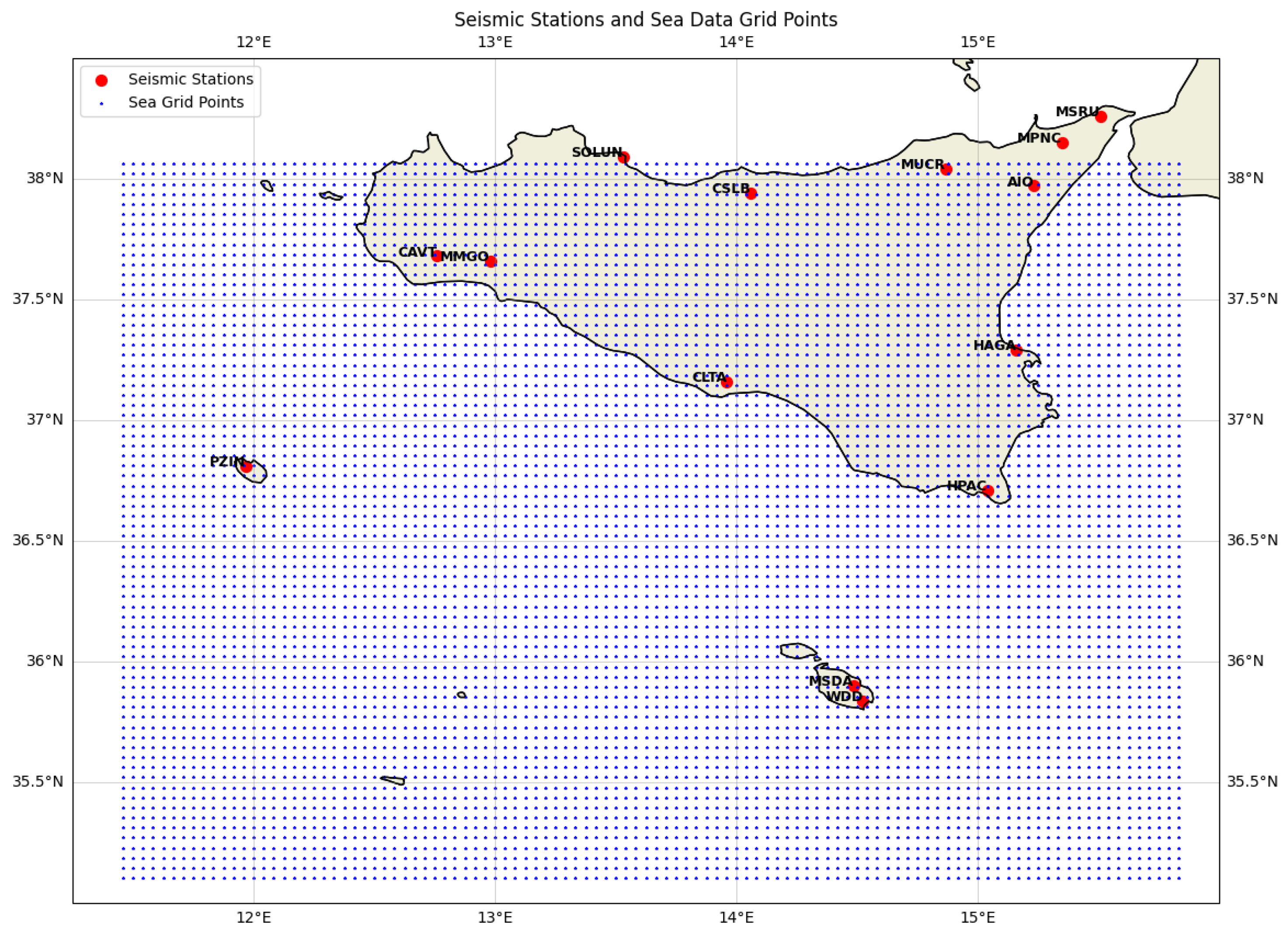
Figure 2.
The region of interest considered in this resesarch.
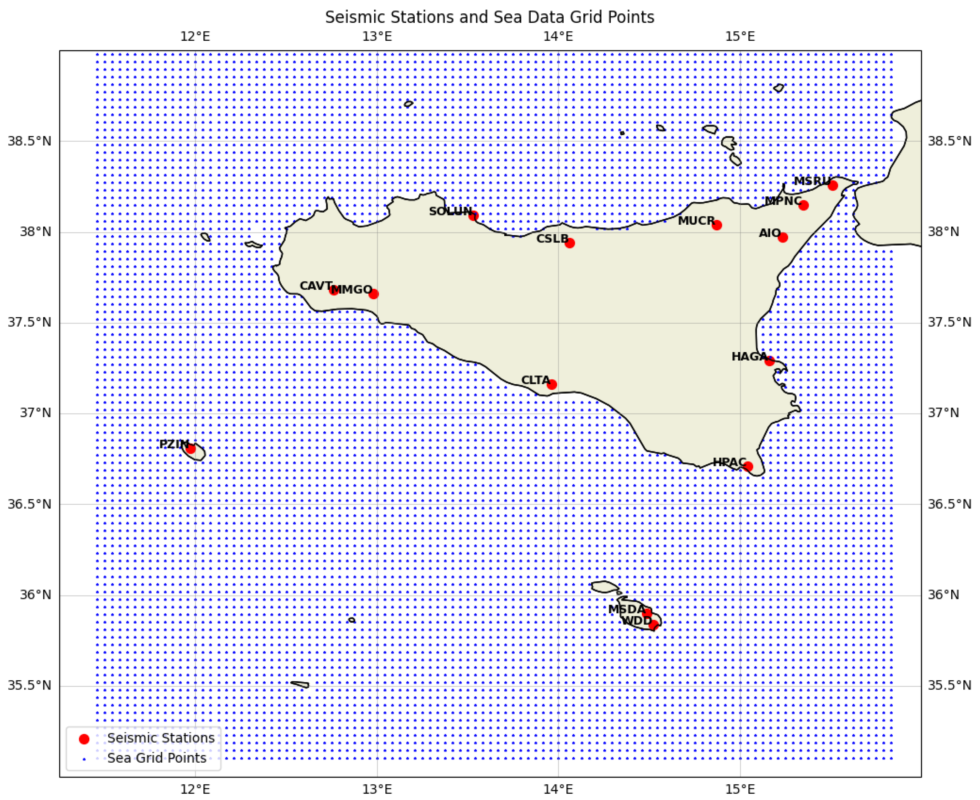
Figure 3.
Predicted and actual time series at station MSDA.
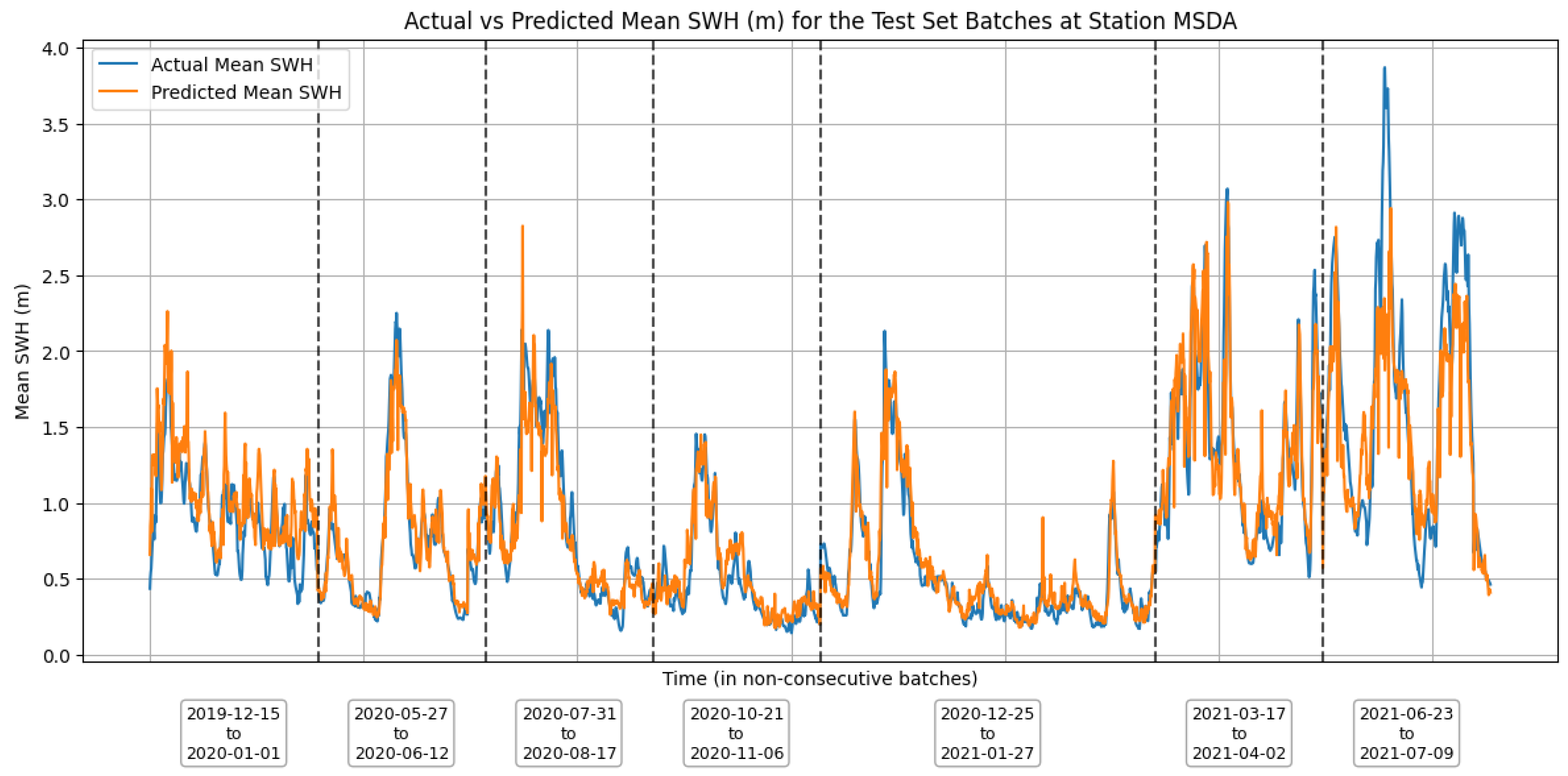

Table 1.
Baseline model performance and final model performance, where the target variable is the mean SWH of the five nearest grid cells.
Table 1.
Baseline model performance and final model performance, where the target variable is the mean SWH of the five nearest grid cells.
| Replicated Baseline Performance | Final Model Performance | |||||||
| Station | R² | MSE | MAE | RMSE | R² | MSE | MAE | RMSE |
| AIO | 0.350 | 0.089 | 0.209 | 0.298 | 0.607 | 0.071 | 0.182 | 0.267 |
| CAVT | - | - | - | - | 0.892 | 0.023 | 0.101 | 0.151 |
| CSLB | 0.868 | 0.044 | 0.137 | 0.210 | 0.881 | 0.055 | 0.143 | 0.235 |
| HAGA | 0.639 | 0.065 | 0.156 | 0.255 | 0.784 | 0.064 | 0.153 | 0.252 |
| MMGO | 0.330 | 0.252 | 0.243 | 0.502 | - | - | - | - |
| MPNC | 0.861 | 0.030 | 0.109 | 0.174 | - | - | - | - |
| MSDA | 0.843 | 0.056 | 0.147 | 0.237 | 0.862 | 0.033 | 0.122 | 0.182 |
| MUCR | 0.840 | 0.052 | 0.156 | 0.228 | 0.862 | 0.041 | 0.141 | 0.202 |
| SOLUN | 0.698 | 0.054 | 0.135 | 0.233 | - | - | - | - |
| WDD | 0.841 | 0.067 | 0.157 | 0.258 | 0.921 | 0.021 | 0.102 | 0.144 |
Table 2.
Optimal hyperparameters selected for each station and corresponding evaluation metrics.
| AIO | CAVT | CSLB | HAGA | MSDA | MUCR | WDD | |
| RF_max_depth | 30 | 30 | 10 | 20 | 30 | 30 | 10 |
| RF_n_estimators | 200 | 200 | 200 | 100 | 100 | 100 | 100 |
| RF_max_features | sqrt | sqrt | 0.5 | ||||
| RF_min_samples_split | 2 | 2 | 5 | 2 | 10 | 10 | 5 |
| RF_min_samples_leaf | 1 | 1 | 3 | 1 | 1 | 1 | 3 |
| MAE | 0.18243 | 0.10066 | 0.14298 | 0.15251 | 0.12207 | 0.14089 | 0.10175 |
| MSE | 0.07107 | 0.02291 | 0.05519 | 0.06361 | 0.03282 | 0.04067 | 0.02073 |
| RMSE | 0.26659 | 0.15137 | 0.23492 | 0.25221 | 0.18116 | 0.20166 | 0.14398 |
| R² | 0.60686 | 0.89238 | 0.88108 | 0.78357 | 0.86198 | 0.86200 | 0.92060 |
Disclaimer/Publisher’s Note: The statements, opinions and data contained in all publications are solely those of the individual author(s) and contributor(s) and not of MDPI and/or the editor(s). MDPI and/or the editor(s) disclaim responsibility for any injury to people or property resulting from any ideas, methods, instructions or products referred to in the content. |
© 2025 by the authors. Licensee MDPI, Basel, Switzerland. This article is an open access article distributed under the terms and conditions of the Creative Commons Attribution (CC BY) license (http://creativecommons.org/licenses/by/4.0/).
Copyright: This open access article is published under a Creative Commons CC BY 4.0 license, which permit the free download, distribution, and reuse, provided that the author and preprint are cited in any reuse.


