Submitted:
30 July 2025
Posted:
31 July 2025
You are already at the latest version
Abstract
A quantum-inspired machine learning framework based on the Heisenberg uncertainty principle is presented in this article. First, we will give the geometric interpretation of the Heisenberg uncertainty principle. Second, the derived uncertainty relation is used to construct a machine learning model, named Heisenberg Bases. The computational experiments demonstrate that the proposed model's performance is comparable to that of the conventional FNN, GRN, RNN, and Transformer, as shown in three case studies. Moreover, a neural-based cell automata created from the Heisenberg bases is introduced and demonstrated in two use cases.
Keywords:
Physics-informed Machine Learning
; Neural Networks
; Quantum Mechanics
; Mathematical Modeling
; Simulation
1. Introduction
Quantum Computing is a cutting-edge field that leverages the principles of quantum mechanics to perform computations far beyond the capabilities of classical computers. Quantum computers utilize qubits, which can exist in multiple states simultaneously (superposition) and are interconnected through quantum entanglement. This allows for parallel processing at an unprecedented scale, offering the potential to revolutionize fields like cryptography, optimization, and material science.
Physics-Informed Machine Learning (PIML) integrates physical laws and principles into machine learning models to enhance predictive capabilities and improve generalization. By incorporating constraints from fields like quantum mechanics, fluid dynamics, or thermodynamics, PIML ensures that models adhere to known physical phenomena, making them more robust and interpretable in applications such as scientific computing, engineering, and environmental modeling.
The rapidly evolving field of quantum machine intelligence can—somewhat humorously—be summarized into three major directions. The first involves implementing classical machine learning algorithms on quantum computers, aiming to harness quantum advantages such as parallelism and entanglement. The second focuses on hybrid approaches, where classical algorithms assist quantum processes. In my prior work, I developed a circuit architecture search algorithm called QES, which uses graphical representations to efficiently search for optimal quantum entangling layouts [1]. The third direction emphasizes the development of native quantum algorithms tailored for quantum systems. By exploiting the probabilistic nature of the quantum wavefunction, I proposed a Bayesian quantum neural network (BayesianQNN) for classification tasks [2], and later introduced a game-theoretic framework known as the Duality Game for modeling dynamical interactions [3]. This framework was further extended to address the problem of biomarker identification in medical applications. A key challenge in this area lies in data encoding for quantum systems, which led to further contributions focused on efficient quantum data representation [4,5].
The main theme of this article is Quantum-inspired machine learning (QIML), a paradigm where the physical laws of quantum mechanics constrain models. QIML differs from QML as the former is a classical neural network inspired by quantum mechanics, while the latter is a machine learning algorithm on quantum computers. PIML differs from classical NN since the model weights (degrees of freedom) are constrained to represent the physics of quantum systems.
Our contribution is three-fold:
- We will propose a new PIML framework that develops machine intelligence grounded in quantum physics;
- We will develop AI models inspired by the Heisenberg uncertainty principle, referred to as HeisenbergBases;
- The proposed model is powerful for representation learning, demonstrating superiority over classical neural network architectures, as numerically validated in three case studies.
The setting for numerical demonstration is designed for low-limited datasets, i.e., a small number of observations. The proposed model is generally compatible with or better than classical neural architectures such as FNN, GRN, RNN, and Transformer models.
This article is organized as follows:
- Section 2 introduces our proposed framework of QIML based on the Heisenberg uncertainty principle of quantum mechanics. We will start with the geometric interpretation of this uncertainty principle in Section 2.1. Then, we will give an implementation of AI models using our derivatives in Section 2.4.
- Section 3 reports the performance of our model compared with FNN, GRN, RNN, and Transformer models in three case studies: (1) quantum state learning, (2) estimation of temperature-solubility in and , (3) spectral classification of materials. We also introduce how to create a cell automaton from the Heisenberg basis model.
- Section 5 discusses the link of our derivation to the original Heisenberg picture. Then, we will emphasize how our proposed model differs from the classical NN. Finally, several future directions are discussed.
2. The Proposed Framework
2.1. Geometric Interpretation of the Heisenberg Uncertainty
Given a pyramid in coordinates with edge length . Imagine an observer moves along the side looking straight into the origin O, and their position on is a point T (Figure 1(A), top panel). The observation plane is . In this setting, the observer can measure the area of the two triangles
The perceived area by the observers changes due to the coordinate of T. For example in the bottom panel of Figure 1(A):
- , the observer fully see the plane and so the area of is fully measured. When the observer is at point A, they have a complete view of triangle , meaning that is fully measured while is not.
- , the observer fully see the plane and so the area of is fully measured. When the observer is at point B, they fully see triangle , meaning is fully measured, but is not.
- When T moving from A to B, the area of increases while that of decreases.
The observer cannot simultaneously fully measure and . As the observer moves from A to B, the measured area of increases while that of decreases, much like the uncertainty relationship: a more precise measurement of one triangle corresponds to a less precise measurement of the other. This mirrors the idea of uncertainty in quantum systems, where the precise measurement of one variable (e.g., position) leads to increased uncertainty in the measurement of its complementary variable (e.g., momentum). In the geometrical analogy, the observer’s inability to fully measure both areas simultaneously represents the inherent trade-off between precision in complementary measurements.
2.2. Derivation of Parameterized Uncertainty
Let be the manifold parameterized by denoted as . We consider to be linked with the Heisenberg uncertainty. We denote
- as a function obtained by project M onto .
- as a function obtained by project M onto .
The area under the curve and are the area of and ; respectively, measured by the observers (Figure 1(B)). We have
When , the upper bound of the integrals is the same, which implies . We can rewrite
Let
where is the multivariate distribution of . The conditional probability of x (position) and p (momentum) being measured are and , respectively. Plugging-in Eq. 3, we have
Here, we assume that and are random variables that change w.r.t time t. Besides, we set
and assume that x and p are random variables from and assumes t is from . If and are independent, their joint distribution is
Moreover, x and p are depend on t by relations and . Using the Bayesian rule, we obtain
or
We have
Simplifying the term and , we have
Since u is just the unit of (recalled that ), we can set and the term
Clearly, and are random variables, assumed that and from the same distribution ; then, the integral returns the expectation of and , says
As a result, we have
and
which directly implies
and
Applying the Cauchy-Schwarz inequality, we have
where
and
The normalization of is computed by
-
Compute the integral of over all x and p:This integral can be separated into two Gaussian integrals:Each integral is a Gaussian integral of the form:
-
Here, . Therefore:So, the total integral is:
-
To normalize , divide it by this integral:Simplify the fraction:
Of note, the multivariate probability is the density function due to the normalization, i.e., it is some joint distribution of . Thus, the integral can be given as
Geometric Relation Between and : The quantities and can be projected onto , say the projected point of and are and . Besides,
- and
- , where .
Therefore,
Given the expressions for and as:
We denoted the modified Heisenberg relation , given as
where:
- is a bounded function in ,
Figure 2.
The value of from our proposed probabilistic sampler
2.3. Our Postulation
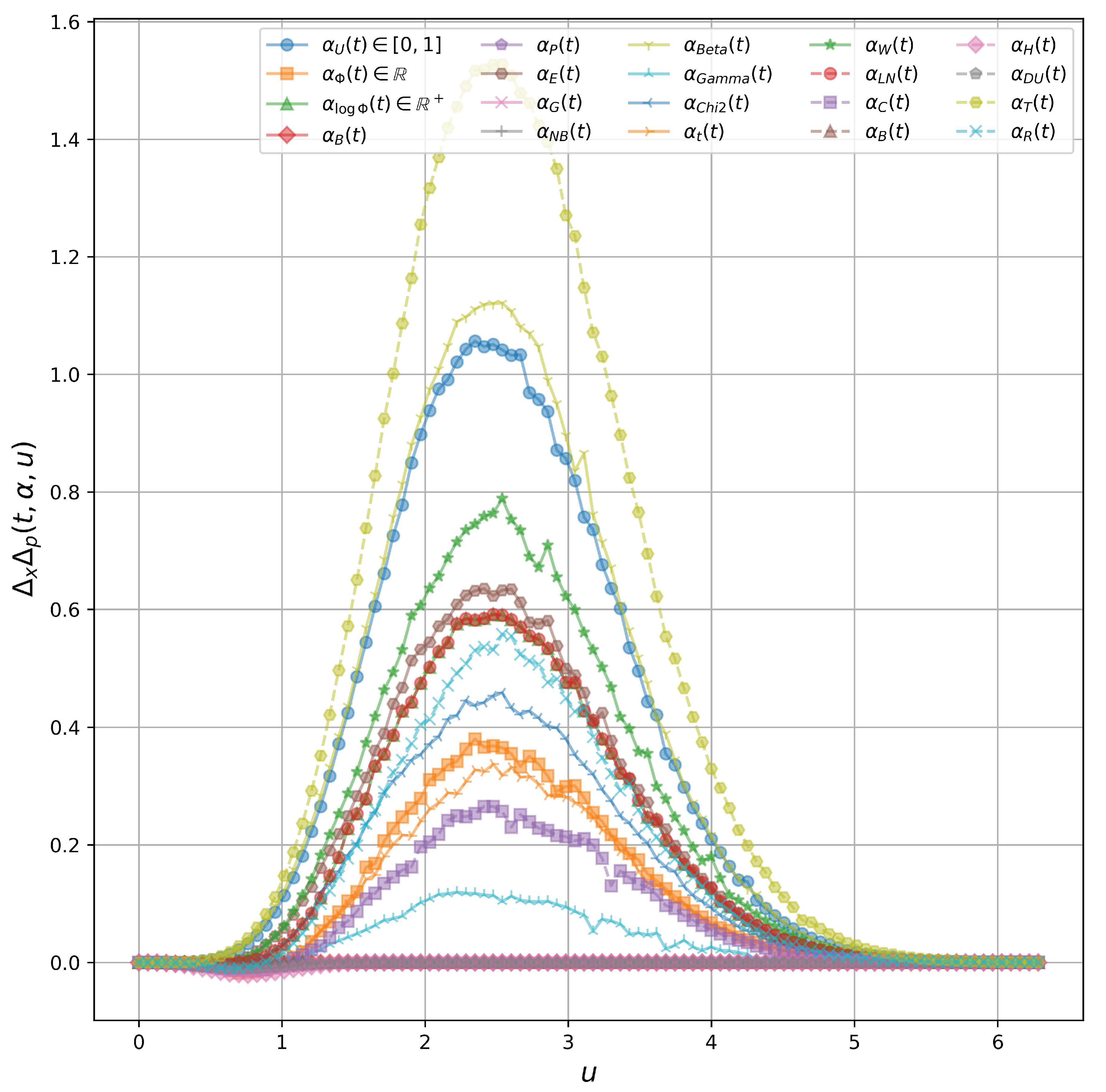
In the Heisenberg uncertainty, the product is a constant lower bound. Here, we postulate that this product is a function of time t, the time-dependent action bounded in , and unit of measurements u. We test seven bounded function for , given in Figure 3, including and (uniformly distributed). There are three main observations:
- Not all bounded function gives a physical sense. Specifically, using result in negative . In fact, and .
- There exist classes of functions with positive . Specifically, other functions (except ) satisfies the above physical constraint, so as scaled functions by a positive scalar.
- When in a random variable from the uniform distribution , we find that not only has lower bound as the Heisenberg uncertainty principle but also has the upper bound, showed as in Figure 3.
These findings contribute to understanding how bounded time-dependent actions influence the uncertainty product, showing that specific classes of functions for can maintain the physical constraints of the Heisenberg uncertainty principle while revealing the existence of an upper bound in certain cases.
2.4. The Proposed Model HeisenbergBases
This section will introduce a neural network model based on the class of functions . It is observed that the values of the function depend on the generating probability distribution for . We create the array
using the same values of t and u. The summary of all generating distribution functions is reported in Table 1.
Given an input matrix where N is the number of samples and D is the number of features, we compute the embedding
The classification layer is a common MLP , which gives the prediction . We name this neural network HeisenbergBases since it is based on our derived uncertainty constraint.
2.5. Quantum State Learning
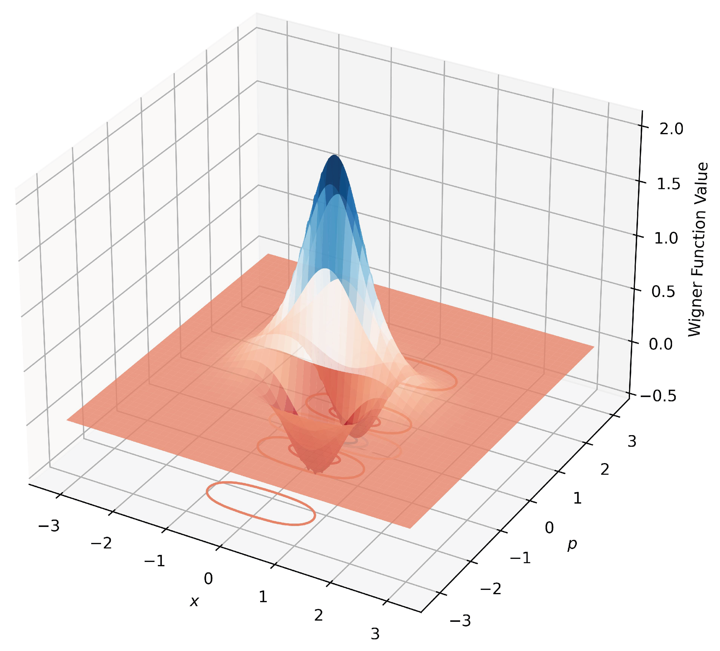
The Wigner function for a coherent state is given by:
The Wigner function for the superposition of two coherent states (Schrödinger’s cat state) is defined as:
We use for the synthesized data. The performance of different models is compared using hypothesis tests with the quantum cat state learning task, reported in Fig Figure 4.
For FNN vs. HeisenbergBases, the p-value is , which is higher than , indicating no significant difference in performance between these models. In the comparison of GRN vs. HeisenbergBases, the p-value is , again showing no significant difference. However, for RNN vs. HeisenbergBases, the p-value is , which is below the threshold, indicating that HeisenbergBases performs significantly better than the RNN model. Lastly, the Transformer vs. HeisenbergBases comparison yields a p-value of , indicating no significant difference in their performance. HeisenbergBases shows relatively competitive performance with FNN and GRN across several loss functions. HeisenbergBases exhibits low variability (low standard deviation) compared to all other models (Fig Figure 4(B)). It has a higher variance than GRN across most loss functions, while RNN and Transformer show lower variance than HeisenbergBases. In AppTable 2, we have enough statistical evidence to show that HeisenbergBases’s performance is better than RNN and Transformer, comparable to FNN and GRN.
2.6. Applications in Material Science
BigSolDB [7] contains solubility values, 830 unique molecules, and 138 individual solvents within the temperature range from to at atmospheric pressure. The dataset consists of six columns, which are explained as follows:
- SMILES — SMILES representation of a dissolved compound
- T,K — Temperature in Kelvin
- Solubility — Experimental solubility value (mole fraction)
- Solvent — Name of the solvent
- SMILES_Solvent — SMILES of the solvent
- Source — A data source for the given values
We use the temperature and solubility values for the model evaluation.
2.6.1. Estimation of Temperature-Solubility Relation
In Table 3, the performance of different models is compared using hypothesis tests on the BigSol dataset. For FNN vs. HeisenbergBases, the p-value is , indicating no significant difference in performance between these models. Similarly, the comparison of GRN vs. HeisenbergBases gives a p-value of , showing no significant difference. However, for the comparison of HeisenbergBases vs. RNN, the p-value is , which is below the threshold, indicating that the HeisenbergBases model significantly outperforms the RNN. For Transformer vs. HeisenbergBases, the p-value is , also indicating a significant difference, with the HeisenbergBases model performing better. Overall, HesenbergBases is the best model in this case study, significantly outperforming all others.
2.6.2. Spectral Classifications of Materials
Spectral data from aluminum, stainless steel, mild steel, copper, and wood were gathered using a spectrometer with advanced on-chip filtering [8]. This spectrometer, featuring a compact 9x9mm array of up to 8 wavelength-selective photodiodes, divides the spectrum into eight bands ranging from 400 to 1100 nm. The goal is to use ML/DL models to learn useful patterns for each material. This evaluation only considers 100 observations of - and -diode. HesenbergBases shows the strongest performance overall, while other models like FNN, GRN, and RNN show minimal performance differences.
In Table 4, the performance of different models is compared using hypothesis tests on the Al-diode dataset. For FNN vs. HeisenbergBases, the p-value is , showing no significant difference between the models. In the comparison of GRN vs. HeisenbergBases, the p-value is , indicating no significant difference. However, in comparisons where HeisenbergBases is the better model—against FNN, GRN, RNN, and Transformer—the p-values are all smaller than , signifying that the HeisenbergBases model significantly outperforms each of these models.
In Table 5, the performance of different models is compared using hypothesis tests on the Cu-diode dataset. HeisenbergBases is compared to FNN, GRN, RNN, and Transformer; the p-values are all very small, with values of , , , and , respectively, indicating that HeisenbergBases significantly outperforms all these models.
Overall, the HeisenbergBases model shows significantly better performance than the FNN, GRN, RNN, and Transformer models, as indicated by the very small p-values in these comparisons. Meanwhile, the FNN, GRN, RNN, and Transformer models show no statistically significant differences in performance when compared with each other.
2.7. Cell Automata
In this section, we will demonstrate that the derived Heisenberg bases can be used as the cell decay rate in cell automata. From Figure 2, we observe that the Heisenberg bases can represent the Black body radiation, which describes the electromagnetic radiation emitted by a perfect black body. It is an idealized physical object that absorbs all incident radiation and emits energy based on temperature. Specifically, associate u as the wavelength and as the spectral radiance. We find that the radiance decays as we increase the wavelength. We will generally use the Heisenberg bases as the decay rates for the cell’s viability.
2.7.1. Dynamical Simulation for Two Competitive Creatures
This model simulates the evolution of a grid-based, 2D system in which cells can be in one of three states: Healthy, Tumor, or Empty. The Simulation proceeds over a specified number of iterations, with each cell’s state updated based on its current state and the states of its neighboring cells. The model includes parameters to control the behavior of cell transitions, including decay and proliferation rates. The simulation begins with a square grid of size , where each cell can represent a healthy cell, a tumor cell, or a space. The system evolves over a specified number of iterations, iter, simulating dynamic changes in cell states. Although the total simulation time t is provided, it does not influence the current model behavior. At each time step, the grid is updated based on local interactions. The transition of each cell depends on its type and the state of its neighbors. Two key factors govern the changes: a decay factor , which controls how likely tumor cells decay into empty spaces, and a proliferation factor , which regulates the growth of healthy cells. Healthy cells remain stable unless a rare event (with 1% chance) causes them to become tumor cells if nearby tumors exist. Tumor cells can decay into space based on the decay factor or persist under certain neighborhood conditions. Empty spaces, in turn, may transform into tumor or healthy cells if surrounded by exactly three tumor or healthy neighbors, respectively, depending on random chance and the associated growth rates. This model captures the competitive spatial dynamics between tumor spread, healthy tissue resilience, and vacant space. As shown in Figure 5, the simulation typically trends toward a dominance of healthy cells, with space reaching a steady-state level by the end of the simulation.
3. Case Studies
4. Experiment Design
4.1. Experimental Environment
The input data is for each of the following experiments. First, we split the data into two independent train and test sets (with ratio ), with the statistics summarized in Table 6. The number of observations is small, similar to practical scenarios. We train a model to reach the minumum of six objective functions : (1) MSE, (2) L1 Loss, (3) smooth L1, (4,5,6): Huber Loss of . We evaluate how well these models can reconstruct the original signals. Specifically, we aim to solve
The smaller loss means the closer distance between the predicted vector and the input , so a good model is obtained. We build the model using torch, and the hyperparameter optimization is performed by optuna. Each neural architecture is trained using 50 epochs under 10 trials of hyperparameter optimization. We use AdamW [6] optimizer with a learning rate of . Random seeds are set for each run. All experiments were conducted with Python 3.7.0 using an Intel i9 processor (2.3 GHz, eight cores) and 16GB DDR4 RAM.
4.1.1. Simulation of Hydrogen’s Electron Orbit
We design an automata model for a 3D model, which simulates the electron’s position in the Hydrogen atom. First, we create a polar grid of coordinates. The cell is active when the electron is present; otherwise, it is inactive. We show the simulation result in Figure 6, colored by the value . The low values are in blue, and the high ones are in red. The update rule is given as if a random value < decay rate, newcells[i, j, k] = 1 - cells[i, j, k] (Flip state (0 to 1 or 1 to 0)). In Figure 6, the electron with high values of r is in the outer region, while the smaller values are closer to the proton. Besides, we can use vertical and horizontal surfaces to stratify the position by and .
Figure 7.
Generating Wigner functions of Quantified Quantum Coherent States
5. Discussion
5.1. The Link to the Heisenberg uncertainty
Since both and is assumed to be positive, we have
5.2. Future Works
5.2.1. Scalability of the model
Adding more generative functions results in more complex Heisenberg bases at the expense of higher computation time. This could lead to a better model as we provide a more general class of random functions. Parallel computing can reduce execution time and mitigate the increased computational cost.
5.2.2. Further Applications
The proposed models can be benchmarked in other learning tasks and datasets. Additionally, cellular automata can be applied to practical applications in biomedical science, physics, chemistry, and machine intelligence. Furthermore, the stochastic electron density models can be utilized for problems in atom and molecular dynamics or quantum chemistry.
5.2.3. Limitations
The proposed model’s universal approximation capability remains uncertain and warrants further investigation in future work. The simulation time for the cellular automata is notably high, necessitating methods to reduce computational costs. We view this work as a preliminary effort to bridge quantum theory with modern machine intelligence. Future research should focus on exploring more intriguing quantum phenomena, such as quantum tunneling and quantum entanglement.
6. Conclusion
To this point, we have introduced a framework to construct AI models based on the parameterized uncertainty (Section 2.4). The uncertainty function is derived from our geometric interpretation in Section 2.1. Three use cases of our proposed framework are demonstrated, which concern applications in quantum computing, material science, and cell automata modeling (Section 3). Some insights into the proposal and its future extensions are also discussed in the article.
Abbreviations
| FNN ∣ Feed-forward Neural Network(s) |
| GRN ∣ Gated Relation Networks(s) |
| ML ∣ Machine Learning |
| NN ∣ Neural Networks |
| PIML ∣ Physics-Informed Machine Learning |
| QIML ∣ Quantum-Informed Machine Learning |
| QML ∣ Quantum Machine Learning |
| RNN ∣ Recurrent Neural Networks(s) |
| Mathematical Notations |
| Oxyz ∣ 3D coordinate |
| u ∣ unit length |
| A, B, C,… ∣ point(s) |
| OA, OB, OC, AB,… ∣ Segment(s) |
| ∣ Manifold |
| S ∣ Area |
| ϕ, ψ, κ, ψ α, … ∣ function(s) |
| x, p, t,… ∣ Variable(s) |
| ∣ Expectation |
| μ ∣ mean |
| σ ∣ standard deviation |
| Λ ∣ Array of bases |
| h ∣ Latent embeddings |
| X, y ∣ Latent embeddings |
| Re, Im ∣ Real and imaginary part of comple number |
References
- Nguyen, N.; Chen, K.C. Quantum embedding search for quantum machine learning. IEEE Access 2022, 10, 41444–41456. [Google Scholar] [CrossRef]
- Nguyen, N.; Chen, K.C. Bayesian quantum neural networks. IEEE Access 2022, 10, 54110–54122. [Google Scholar] [CrossRef]
- Nguyen, P.N. The duality game: a quantum algorithm for body dynamics modeling. Quantum Information Processing 2024, 23, 21. [Google Scholar] [CrossRef]
- Nguyen, P.N. Quantum word embedding for machine learning. Physica Scripta 2024, 99, 086004. [Google Scholar] [CrossRef]
- Nguyen, P.N. Quantum DNA Encoder: A Case-Study in gRNA Analysis. In Proceedings of the 2024 IEEE 48th Annual Computers, Software, and Applications Conference (COMPSAC). IEEE, 2024; pp. 232–239. [Google Scholar]
- Loshchilov, I. Decoupled weight decay regularization. arXiv preprint arXiv:1711.05101, 2017. [Google Scholar]
- Krasnov, L.; Mikhaylov, S.; Fedorov, M.; Sosnin, S. BigSolDB: Solubility Dataset of Compounds in Organic Solvents and Water in a Wide Range of Temperatures 2023.
- Bhatt, T.; Soni, R.; Upadhyay, M.; Jayswal, H.; Chaudhari, J.; Dubey, N.; Patel, A.; Sharma, S.; Makwana, A. A Spectral Dataset of different materials for metal classification 2024.
Figure 1.
Geometric Interpretation of the Heisenberg Uncertainty
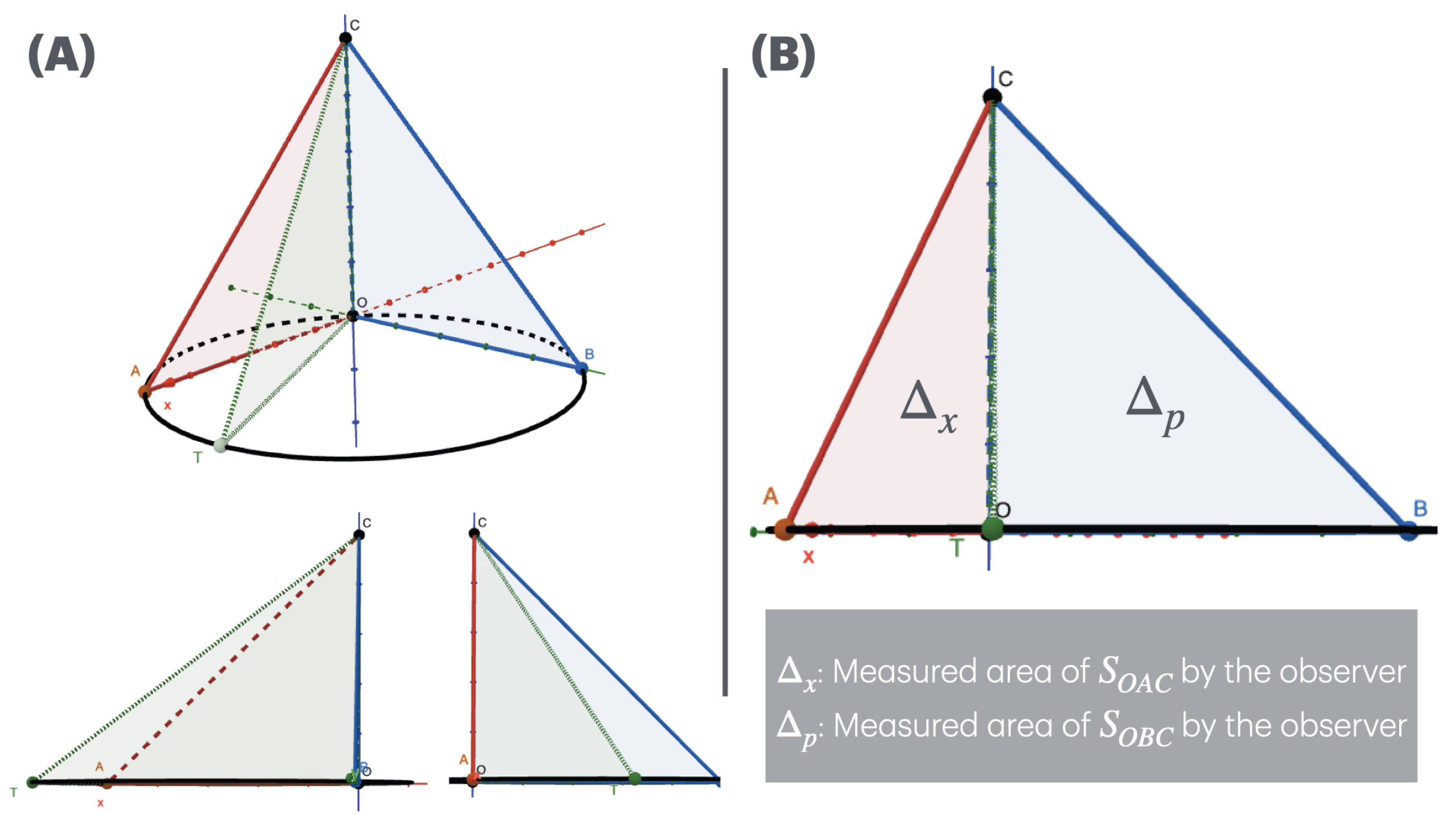
Figure 3.
The value of w.r.t unit of measurement , is a bounded function in and
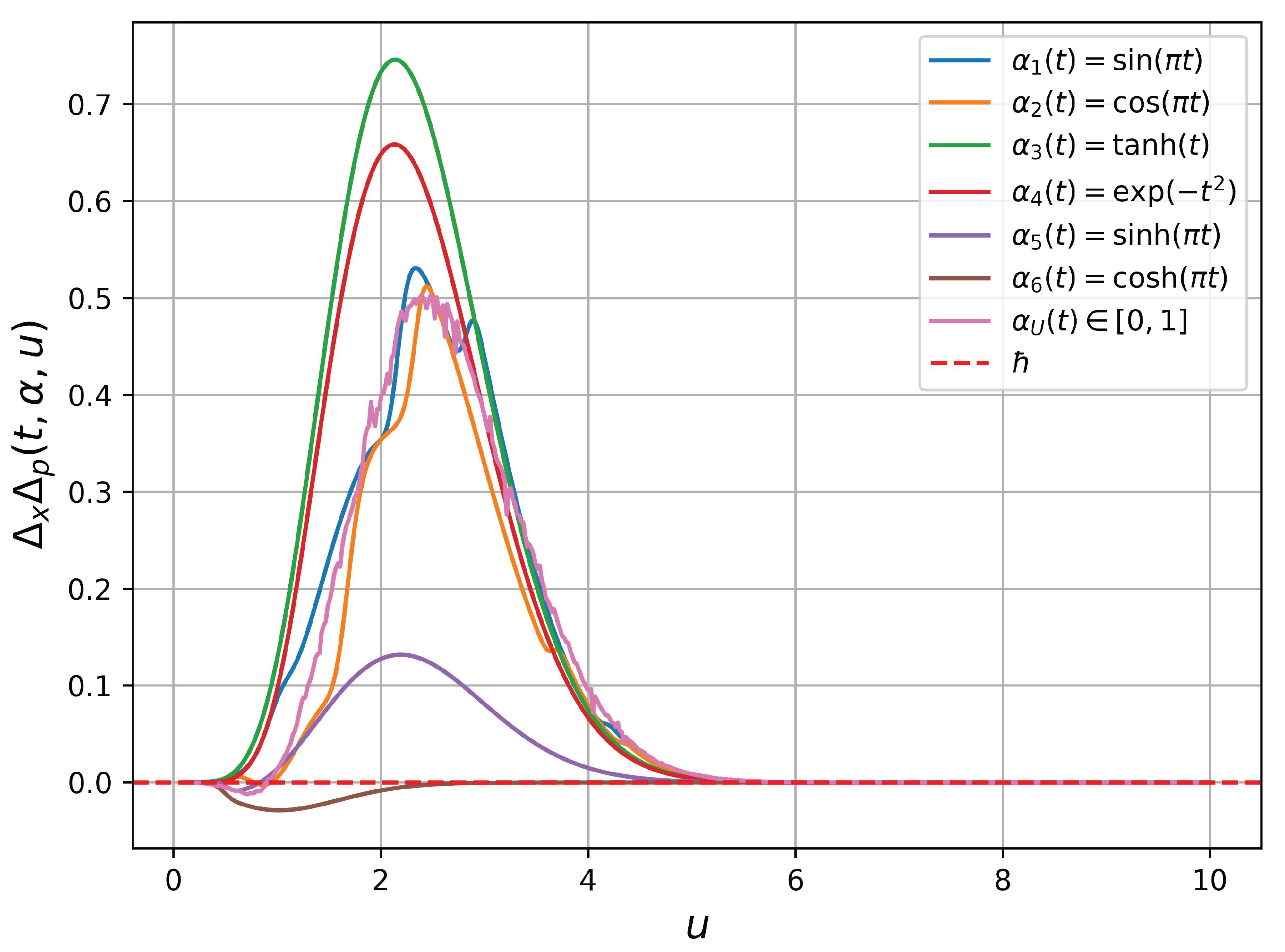
Figure 4.
Evaluation in quantum state learning task. (A) mean loss, (B) standard deviation of loss.
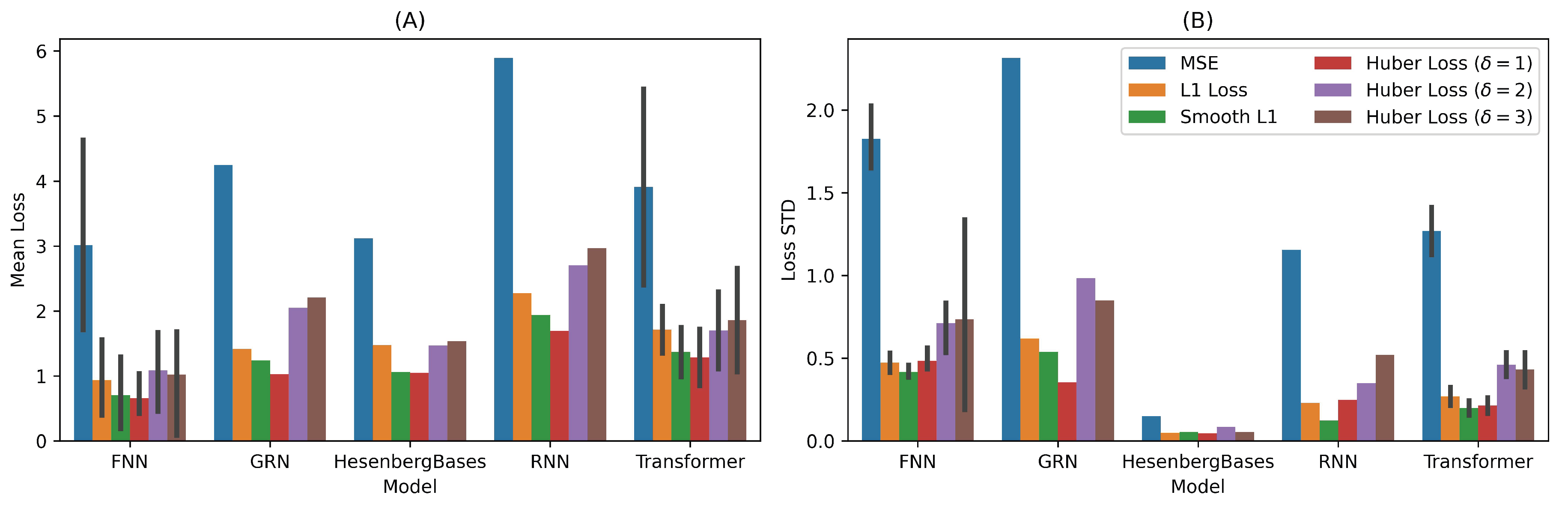
Figure 5.
Cell automata model of tumor-healthy cells competition. Left: spatial distribution of tumor (red), healthy (blue), and empty cells (white). Right: cell counts over time
Figure 5.
Cell automata model of tumor-healthy cells competition. Left: spatial distribution of tumor (red), healthy (blue), and empty cells (white). Right: cell counts over time
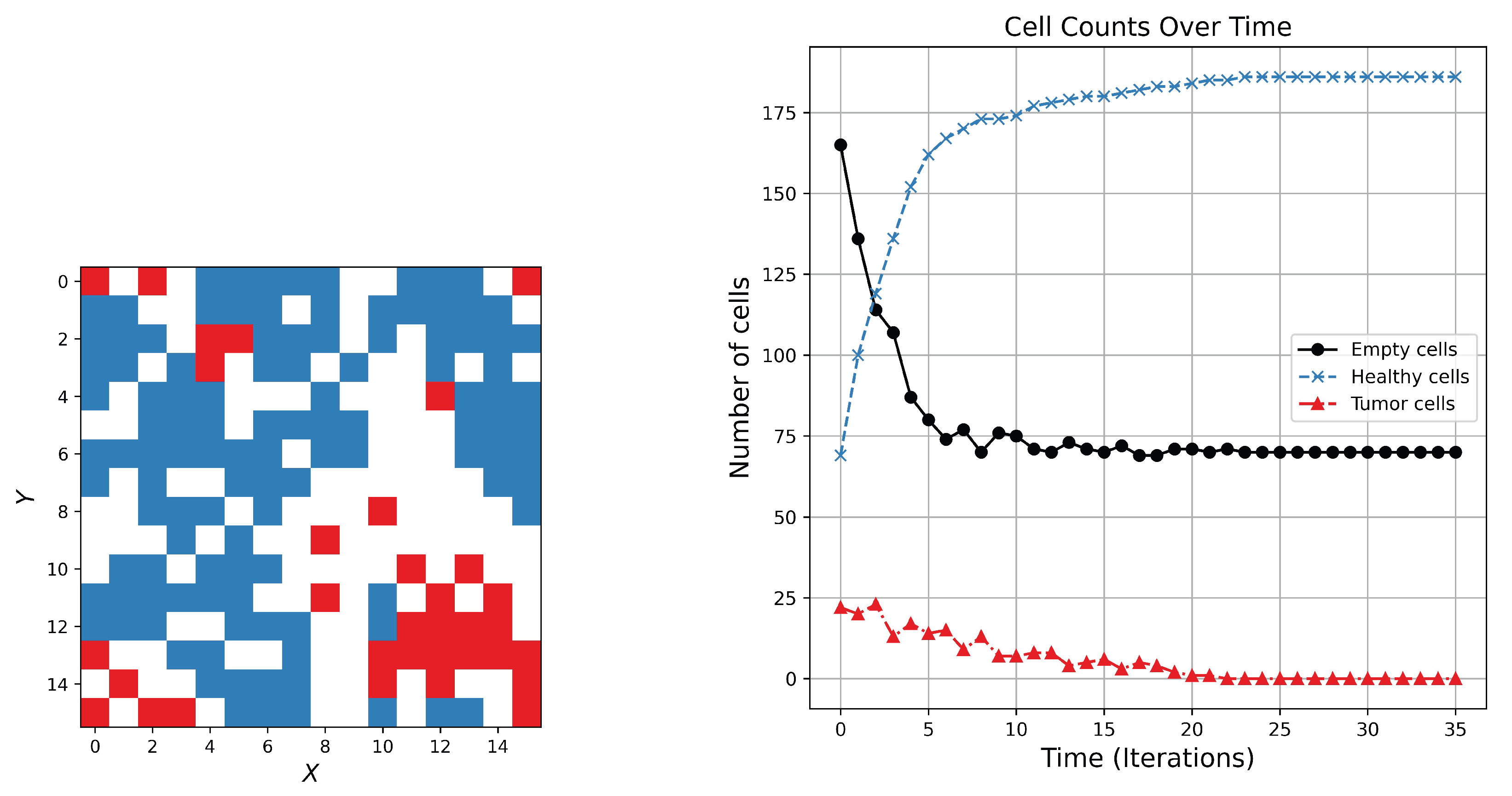
Figure 6.
Simulation of hydrogen’s electron orbit
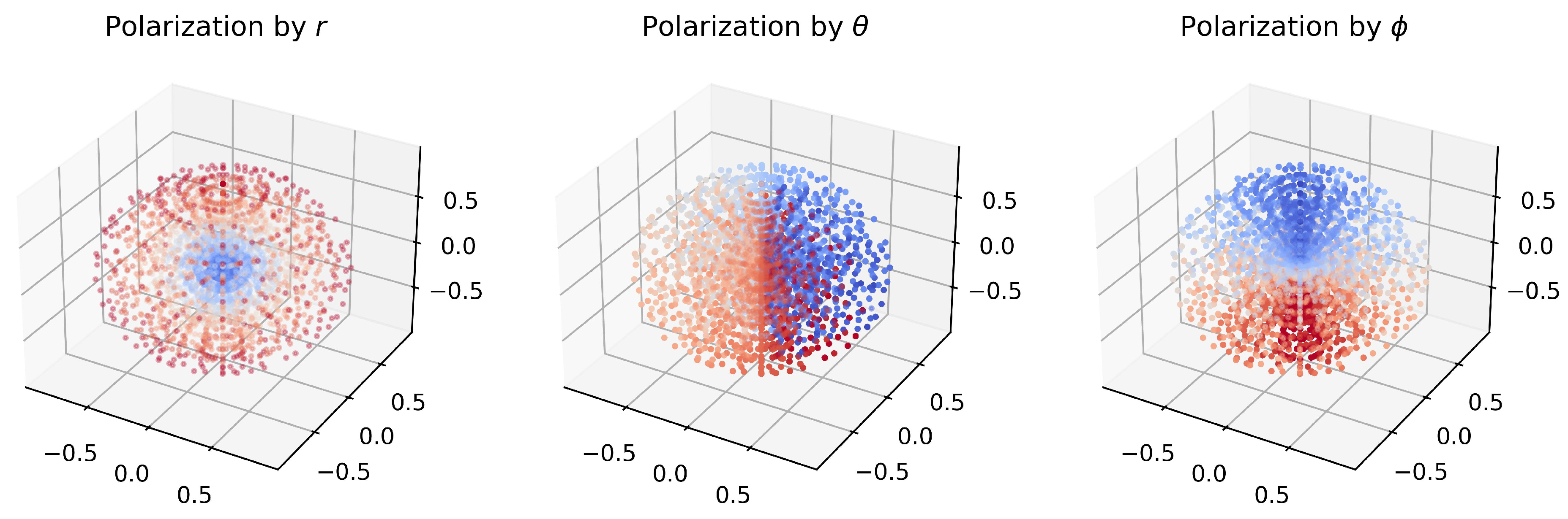

Table 1.
The generating distribution used in our HeisenbergBases
| Distribution Name | Mathematical Eqtion |
|---|---|
| Uniform | |
| Normal | |
| Binomial | |
| Poisson | |
| Exponential | |
| Geometric | |
| Negative Binomial | |
| Beta | |
| Gamma | |
| Chi-squared | |
| Student’s t | |
| Weibull | |
| Lognormal | |
| Cauchy | |
| Bernoulli | |
| Hypergeometric | |
| Discrete Uniform | |
| Triangular | |
| Rayleigh |
Table 2.
P-value of statistical test among model’s average performance in quantum cat state learning task
Table 2.
P-value of statistical test among model’s average performance in quantum cat state learning task
| Hypothesis Test | p-value |
|---|---|
| FNN < GRN | 0.0518 |
| FNN < HesenbergBases | 0.1398 |
| FNN < RNN | 0.0007* |
| FNN < Transformer | 0.0146* |
| GRN < FNN | 0.9552 |
| GRN < HesenbergBases | 0.6504 |
| GRN < RNN | 0.0898 |
| GRN < Transformer | 0.5542 |
| HesenbergBases < FNN | 0.8746 |
| HesenbergBases < GRN | 0.4091 |
| HesenbergBases < RNN | 0.0206* |
| HesenbergBases < Transformer | 0.3082 |
| RNN < FNN | 0.9995 |
| RNN < GRN | 0.9340 |
| RNN < HesenbergBases | 0.9870 |
| RNN < Transformer | 0.9585 |
| Transformer < FNN | 0.9869 |
| Transformer < GRN | 0.4818 |
| Transformer < HesenbergBases | 0.7234 |
| Transformer < RNN | 0.0512 |
Table 3.
P-value of statistical test among models’ average performance in BigSol dataset
| Hypothesis Test | p-value |
|---|---|
| FNN < GRN | 0.0232* |
| FNN < HesenbergBases | 0.9995 |
| FNN < RNN | 0.0043* |
| FNN < Transformer | 0.0160* |
| GRN < FNN | 0.9798 |
| GRN < HesenbergBases | 0.9999 |
| GRN < RNN | 0.0705 |
| GRN < Transformer | 0.1248 |
| HesenbergBases < FNN | 0.0007* |
| HesenbergBases < GRN | * |
| HesenbergBases < RNN | * |
| HesenbergBases < Transformer | 0.0004* |
| RNN < FNN | 0.9964 |
| RNN < GRN | 0.9370 |
| RNN < HesenbergBases | 0.9999 |
| RNN < Transformer | 0.8546 |
| Transformer < FNN | 0.9878 |
| Transformer < GRN | 0.8936 |
| Transformer < HesenbergBases | 0.9997 |
| Transformer < RNN | 0.1677 |
Table 4.
P-value of statistical test among models’ average performance in Al-diode dataset
| Hypothesis Test | p-value |
|---|---|
| FNN < GRN | 0.3916 |
| FNN < HesenbergBases | 1.0000 |
| FNN < RNN | 0.0328* |
| FNN < Transformer | 0.0328* |
| GRN < FNN | 0.6246 |
| GRN < HesenbergBases | 0.9999 |
| GRN < RNN | 0.0705 |
| GRN < Transformer | 0.0705 |
| HesenbergBases < FNN | * |
| HesenbergBases < GRN | * |
| HesenbergBases < RNN | * |
| HesenbergBases < Transformer | * |
| RNN < FNN | 0.9702 |
| RNN < GRN | 0.9370 |
| RNN < HesenbergBases | 0.9999 |
| RNN < Transformer | 0.9214 |
| Transformer < FNN | 0.9702 |
| Transformer < GRN | 0.9370 |
| Transformer < HesenbergBases | 0.9999 |
| Transformer < RNN | 0.0874 |
Table 5.
P-value of statistical test among models’ average performance in Cu-diode dataset
| Hypothesis Test | p-value |
|---|---|
| FNN < GRN | 0.1552 |
| FNN < HesenbergBases | 0.9999 |
| FNN < RNN | 0.0270* |
| FNN < Transformer | 0.0270* |
| GRN < FNN | 0.8602 |
| GRN < HesenbergBases | 0.9997 |
| GRN < RNN | 0.1454 |
| GRN < Transformer | 0.1454 |
| HesenbergBases < FNN | * |
| HesenbergBases < GRN | 0.0004* |
| HesenbergBases < RNN | * |
| HesenbergBases < Transformer | * |
| RNN < FNN | 0.9755 |
| RNN < GRN | 0.8752 |
| RNN < HesenbergBases | 0.99999 |
| RNN < Transformer | 0.9214 |
| Transformer < FNN | 0.9755 |
| Transformer < GRN | 0.8752 |
| Transformer < HesenbergBases | 0.99999 |
| Transformer < RNN | 0.0874 |
Table 6.
Case studies with training and test data sizes
| Index | Case Study | Ref. | ||
|---|---|---|---|---|
| 1 | Wigner function of Quantum Cat State | 80 | 20 | Simulated |
| 2 | Estimation of Temperature-Solubility Relation | 144 | 37 | BigSolBD [7] |
| 3 | Spectral Classifications of Materials (Al) | 80 | 20 | [8] |
| 4 | Spectral Classifications of Materials (Cu) | 80 | 20 | [8] |
Disclaimer/Publisher’s Note: The statements, opinions and data contained in all publications are solely those of the individual author(s) and contributor(s) and not of MDPI and/or the editor(s). MDPI and/or the editor(s) disclaim responsibility for any injury to people or property resulting from any ideas, methods, instructions or products referred to in the content. |
© 2025 by the authors. Licensee MDPI, Basel, Switzerland. This article is an open access article distributed under the terms and conditions of the Creative Commons Attribution (CC BY) license (http://creativecommons.org/licenses/by/4.0/).
Copyright: This open access article is published under a Creative Commons CC BY 4.0 license, which permit the free download, distribution, and reuse, provided that the author and preprint are cited in any reuse.


