
Submitted:
28 July 2025
Posted:
30 July 2025
You are already at the latest version
Abstract
Coniferous forests in Canada play a vital role in carbon sequestration, wildlife conservation, climate change mitigation, and long-term sustainability. Traditional methods for classifying and segmenting coniferous trees have primarily relied on the direct use of spectral or LiDAR-based data. In 2024, we introduced a novel data representation method, Pseudo Tree Crown (PTC), which provides a pseudo-3D pixel-value view that enhances the informational richness of images and significantly improves classification performance. While our original implementation was successfully tested on urban and deciduous trees, this study extends the application of PTC to Canadian conifer species, including Jack Pine, Douglas Fir, Spruce, and Aspen. We address key challenges such as snow-covered backgrounds and evaluate the impact of training dataset size on classification results. Classification was performed using Random Forest, PyTorch(ResNet50), and YOLO versions v10, v11, and v12. The results demonstrate that PTC can substantially improve individual tree classification accuracy by up to 13% reaching the high 90% range.
Keywords:
Pseudo tree crown (PTC)
; individual tree species (ITS) classification
; unmanned aerial vehicle (UAV)
; deep learning (DL)
; machine learning (ML)
1. Introduction
Forests play a crucial role in maintaining ecological balance, supporting biodiversity, and mitigating climate change [1,2]. In particular, North America’s boreal forests have the potential to serve as climate refugia under global warming conditions, helping to sustain biodiversity and ecosystem resilience [3].
Accurate and detailed tree classification, especially at the individual tree level, is critical for assessing biodiversity, forest health, and sustainable forest management [4,5]. Information on tree species can also provide insights into drought susceptibility and predict height growth trends, aiding in proactive forest conservation strategies [6].
Remote Sensing (RS) has been widely adopted for forest monitoring due to its flexibility, broad coverage, cost-effectiveness, and long-term sustainability [7]. Various RS platforms, including satellite-borne, airborne, unmanned aerial vehicles (UAVs), and ground-based sensors, offer diverse data sources, ranging from visible and multispectral to hyperspectral, high-spatial-resolution, and thermal imaging. Traditionally, RS-based forest analysis has relied on empirical indices and vegetation models across different scales. However, with advancements in machine learning (ML), particularly deep learning, image classification has become more intelligent and automated. Despite these improvements, classification accuracy is highly dependent on training data quality and susceptibility to noise [8,9].
A critical limitation of most RS techniques is their reliance on nadir (top-down) imagery, which lacks vertical structural information essential for forest analysis [10]. My research focuses on addressing this limitation by compensating for the missing vertical information in nadir-view RS imagery data. Over a decade of research and development [11,12] has led to the introduction of the Pseudo Tree Crown (PTC) data representation, a pseudo-3D (or 2.5D) model that strongly correlates with the True Tree Crown (TTC) structure. This paper is part of an ongoing series that applies PTC to contemporary ML approaches. We reported the successful application in deciduous trees [13,14]. This paper expands PTC to coniferous trees, demonstrating its potential to enhance tree classification and forest analysis for more species. The preliminary results of limited Canadian conifer tree studies were reported in [15].
In this study, we selected five ML image classifiers: 1) Random Forest (RF) as the traditional approach benchmark; 2) ResNet50 using the PyTorch framework, which is a widely adopted mainstream classifier; 3) You Only Look Once (YOLO) v10; 4) YOLOv11; and 5) YOLOv12. We are not only comparing the effectiveness of these ML classifiers, but rather examining if adopting PTC can improve the classification. We have achieved a 2 - 12% improvement across all classifiers.
The paper is organized as follows: We briefly review the recent related work in Section 2, focusing mainly on studies from late 2024 and 2025, as most of the earlier work was already covered in our Miao et al. (2024) [14] paper. Section 3 presents our dataset details and preprocessing steps. In Section 4, we report all comparison results and investigate the impacts of both snow background and dataset size. Section 5 provides a discussion of our findings, and we wrap up with a solid conclusion in Section 6.
2. Related Work
2.1. The classic Machine Learning (ML) Classification
The classic machine learning classifiers, such as Support Vector Machine (SVM) [16] and Random Forest (RF) [17], remain widely used in recent research. Their main advantages lie in their relatively low computational cost and simple architecture [18]. A common trend today is to use SVM and RF as benchmark models or integrate them into more complex machine learning frameworks. For example, Hu et al. (2025) [19] applied RF to multispectral airborne LiDAR data for urban tree species classification. Ke et al. (2025) [20] adopted a modified RF approach, MRMR-RF-CV, to classify wetlands using multi-source remote sensing imagery. El Kharki et al. (2024) [21] utilized SVM with Sentinel-2 data for argan tree classification, while Thapa et al. (2024) [22] compared SVM, RF, and neural networks (NN) for urban tree species identification. Wang and Jiang (2024) [23] combined SVM with a Convolutional Neural Network (CNN) to classify trees using hyperspectral imagery. Zhang et al. (2024) [24] employed RF, SVM, and gradient tree boosting (GTB) to explore classification performance differences between Sentinel-2 and Landsat-8 data in Northern and Southern China. Aziz et al. (2024) [25] compared the artificial neural network (ANN) classifier with RF and reported situational strengths for both. Manoharan et al. (2023) [26] proposed a hybrid fuzzy SVM model for coconut tree classification.
2.2. The Deep Learning Classification Progress
CNN was originally introduced by LeCun et al. (1998) [27], while Graph Neural Networks (GNNs) were first proposed by Scarselli et al. (2009) [28]. Krizhevsky et al. (2012) [29] introduced AlexNet, and Simonyan et al. (2014) [30] proposed the Visual Geometry Group (VGG) network, which increased depth by adding layers to improve accuracy. Ronneberger et al. (2015) [31] proposed U-Net, effective for small sample sizes and pixel-level segmentation. He et al. (2016) [32] introduced the revolutionary ResNet based on residual blocks, marking an important milestone for CNNs. He et al. (2017) [33] proposed Mask R-CNN for instance segmentation. Woo et al. (2018) [34] introduced the Convolutional Block Attention Module (CBAM), which enhances feature representation through attention mechanisms. Veličković et al. (2018) [35] proposed Graph Attention Networks (GAT), bringing attention mechanisms to graph classification. Tan et al. (2019) [36] introduced EfficientNet, which applied a compound scaling method to improve model efficiency. Dosovitskiy et al. (2020) [37] introduced the Vision Transformer (ViT), exploring the potential of transformers in image classification. Ren et al. (2021) [38] proposed Rotated Mask R-CNN for oriented object detection. Ding et al. (2022) [39] proposed RepLKNet, which uses large kernels to improve image classification performance.
With the rapid development of CNN models and their application to tree classification, explosive progress has been made. Hundreds of papers have been published, showcasing a wide range of methods and results. A comprehensive summary is available in Zhong et al. (2024) [9]. For example, Wang et al. (2025) [40] proposed TGF-Net, a fusion of Transformer and Gist CNN networks for multi-modal image classification. Chi et al. (2024) [41] introduced TCSNet, designed for individual tree crown classification using UAV imagery. Dersch et al. (2024) [42] applied Mask R-CNN for UAV RGB image classification.
2.3. The You Only Look Once (YOLO) Development
The You Only Look Once (YOLO) family has emerged as one of the most promising object detection frameworks, maintaining its popularity and active development since 2015 when it was first introduced by Redmon et al. [43]. New versions and improvements have been released every few months since 2020, reflecting the community’s commitment to innovation [44,45]. It is important to note that YOLO has been developed and contributed to by various researchers and teams, with version numbers indicating the release order rather than representing effectiveness or direct inheritance.
From the reviews of YOLO from YOLOv1 to YOLOv8 YOLOv5 [44,45], developed by Glenn Jocher and the Ultralytics team in 2020, was the first stable and widely adopted version. It was one of the compared classifiers for our previous research [14], demonstrating competitive performance. YOLOv5 is built upon a Cross Stage Partial (CSP) backbone and a Path Aggregation Network (PANet) for feature fusion. YOLOv8 (2023), also developed by Glenn Jocher and the Ultralytics team, introduced several improvements. It employs a refined CSP backbone and an anchor-free detection head, which enhances adaptability to objects with varying sizes and aspect ratios.
YOLOv10 (2024), proposed by researchers at Tsinghua University using the Ultralytics Python package [46], further refined the CSPNet backbone and introduced a dual-head design: a “one-to-many” head for training and a “one-to-one” head for inference. This version eliminated non-maximum suppression (NMS). As a result, this version significantly reduces inference latency and lowers computational costs [47].
Khanam and Hussain introduced YOLOv11 (late 2024) [48], which departs from earlier versions by adopting a Transformer-based backbone. Its dynamic detection head adjusts processing based on image complexity, enabling optimized use of computational resources.
The latest version, YOLOv12 (early 2025), proposed by Tian et al. [49], employs an attention-centric design. It incorporates an Area Attention module, which enhances detection in cluttered scenes by selectively focusing attention. Additionally, FlashAttention integration reduces memory access bottlenecks, further improving inference efficiency. As if now, the YOLOv13 had also been proposed, but the algorithm and codes are not stable and we did not include that in this study.
While YOLOv5, YOLOv8, and YOLOv10 have been widely used in research and practical applications, YOLOv11 and YOLOv12 are relatively new. Further in-depth studies are needed to fully explore and validate their potential.
3. Data and Preprocessing
3.1. Study Area, Instruments and Data Acquisition
The study area is located south of Kamloops, British Columbia (50°34’19.345"N, 120°27’1.209"W), and represents a typical North American boreal forest mix, as shown in Figure 1. Aerial imagery was captured on February 17, 2023, and uploaded by Arura UAV [50]. The dataset, licensed under Creative Commons (CC) 4.0, was designated as a public project on March 31, 2025.
The survey was conducted using a DJI Zenmuse P1 camera (Shenzhen, China) mounted on a DJI M300 RTK drone (Shenzhen, China) at an average flight altitude of approximately 128 meters. The camera has a 35 mm fixed focal length with a maximum aperture of f/2.8. The shutter speed was set to 1/500 second. All images were georeferenced using the WGS84 coordinate system and saved in JPEG format.
Sample overall image and individual trees from four species: Fir, Pine, Spruce, and Aspen, are illustrated in Figure 2.
4. Methodology
Simply speaking, our study has two steps: we used PTC as a novel input image format, replacing the standard nadir-view images. Then feed into different ML/DL classifers. This is an extension of our earlier work reported; more details of PTC can be found in Miao et al. [14]. The PTC generation workflow is illustrated in Figure 3.
PTC is our original contribution, developed over more than a decade. In this study, we focused on Conifer trees under winter conditions, which required an additional step of snow background removal. We compared classification results with and without this snow removal step, as discussed in Section 5.2. Some samples of individual trees with pre-processing snow background removal are shown in Figure 4.
In the snow background removal step, we filtered out the very high grey value pixels (above 220) and clipped closer to the tree crown. Then convert it to PTC. A sample is shown in Figure 5.
We evaluated the following ML/DL image classifiers: (1) Traditional ML RF as a baseline, illustrated in Figure 6. RF is a widely used ensemble method known for its robustness and interpretability, especially in cases with limited training data. (2) ResNet50, implemented in PyTorch, which previously yielded the best performance in our deciduous tree study (Figure 7). ResNet50 benefits from deep residual learning, making it effective for capturing complex features in tree crowns. The detailed parameter information is listed in Table 1 (3) YOLOv10, (4) YOLOv11, and (5) YOLOv12, the latest version we implmented. These YOLO models represent state-of-the-art object detection architectures, with increasing efficiency and accuracy across versions. The general workflow for YOLO-based models is shown in Figure 8.
While many other classifiers could be explored, we limited our scope to these five due to time constraints and paper length. We encourage researchers to experiment with PTC using their own datasets and preferred models.
5. Results
5.1. The Classification Results of Different Models
We used standard evaluation metrics, including the confusion matrix, Accuracy, Precision, Recall, F1 Score, and Intersection over Union (IoU). The corresponding formulas are shown in Equations (1) to (5), where TP denotes True Positives, TN is True Negatives, FP is False Positives, and FN is False Negatives.
The accuracy results are presented in Table 2 to provide an overall view. Detailed metrics: Precision, Recall, F1 Score, and IoU are shown in Table 3, Table 4, Table 5, Table 6, and Table 7 for RF, PyTorch, YOLOv10, v11, and v12, respectively. The corresponding confusion matrices are illustrated in Figure 9, Figure 10, Figure 11, Figure 12, and Figure 13.
5.2. Snow and Background Removal
Since YOLO can operate without any preprocessing, we tested it both with and without removing the snow background. The results show a significant impact, as presented in Table 8.
5.3. The Classification Results of Different Dataset Sizes
6. Discussion
6.1. General PTC Performance and Effectiveness
Overall, the PTC consistently outperformed the original RGB images across nearly all models we tested, which aligns with the findings from our previous study [14]. This reinforces the idea that the PTC image representation can be effectively incorporated with any ML and DL classifiers. The reasoning is straightforward: the pseudo-3D structure provides an additional information channel for classification. It’s generally easier to extract features from a “shape” than from pixel-level correlations alone. The accuracy improvements ranged from around 2% to as much as 11%, which is quite promising.
That said, we did observe that certain species, Aspen, for example (see Figure 4), were more sensitive to the snow background in winter when they lack foliage. This background interference led to a slight drop in classification robustness, particularly for species with finer structural features. Still, even under these more challenging conditions, the PTC held up reasonably well. This shows that if the background interferes with the PTC view, it can directly affect the classification result. Still, even under these more challenging conditions, the PTC held up reasonably well.
6.2. PTC with Different Models
When comparing model performance, a few interesting patterns showed up. RF surprisingly delivered the best results overall. It’s simple, but it works well with the PTC format. Among the DL models, YOLOv10 outperformed both YOLOv11 and YOLOv12. This isn’t entirely unexpected. Because in YOLO, a version number doesn’t reflect the performance. The higher version number does not mean much. The YOLO had been contributed by research groups, and the version is just the sequence of release order. In fact, YOLOv10 seems to be a much improved and more stable version of YOLOv5, which we previously used successfully in our Deciduous tree study [14]. The newer YOLOv11 and YOLOv12 models didn’t really offer additional advantages in this specific context, possibly due to how they were optimized or trained, which may not align well with PTC-style inputs. Another reason we did not go further on the latest YOLOv13, which just released while we are wrapping up this study.
6.3. PTC Performance: Deciduous vs. Conifer
We also found some clear differences between Deciduous and Conifer tree species classification performance. Deciduous trees, especially in summer, still have full foliage, which helps the model separate the trees from the background. But in this study, Conifer trees in winter posed more of a challenge. With fewer leaves and heavy snow coverage, the background started blending into the tree structure, especially for Trembling Aspen, where the contrast was minimal. In some cases, that snow really muddied the features. Table 8 shows that snow can cause an 8%–15% drop in performance. RGB images, which rely more on color and texture, were hit harder by this. PTC, which captures more structural shape features, was also negatively affected, but less so, with only around a performance drop 6% - 13%. So even in tough conditions, PTC showed some resilience.
6.4. Impact of Dataset Size
Another important factor was the size of the dataset. As expected, the number of training samples played a significant role. PTC generally performed well across all dataset sizes, but with smaller datasets, we observed a few unexpected results. To investigate further, we tested six dataset sizes: 170, 270, 370, 470, 570, and 852 samples, as shown in Table 9, Table 10, Table 11, Table 12, and Table 13. In every case, PTC still outperformed the original RGB format, though the degree of improvement varied.
In RF and PyTorch (ResNet50), increasing the dataset size led to a steady rise in classification accuracy. Interestingly, YOLO-based models showed more variations. For example, YOLOv12 dropped to just 66.8% accuracy at the smallest dataset size, which shows it’s less robust when data is limited. RF, on the other hand, held up much better, its accuracy only varied by about 2% across all sample sizes, which is quite stable. PyTorch (ResNet50) and the other YOLO versions showed 3%–7% variation, which is still decent but not as reliable as RF. These results suggest that if your dataset is on the smaller side, RF or a traditional ML approach may be a better starting point for working with PTC. The YOLO models seemed to hit a threshold around 570 samples, after which the accuracy either saturated or stopped improving. We suspect it may be related to the quality of the training data. This shows that even though PTC can help boost performance, its effectiveness still depends on both dataset size and data quality.
7. Conclusions
In this study, we expanded the use of PTC, a novel way of representing data that transforms traditional top-down (nadir) imagery into more informative pseudo-3D (2.5D) side-view perspectives of trees. This approach shows real potential for improving tree species classification accuracy and estimating 3D biometric parameters, which are critical for effective forest monitoring and management.
We pushed the PTC concept further by applying it beyond just deciduous trees in the summer (like we did in our earlier work) and into the more challenging context of conifers in winter. This lets us explore both the overlap and the differences between these scenarios, structurally and seasonally.
From all the experiments we ran with different ML and DL models, the results were consistent: PTC outperformed the original RGB inputs across the board. That said, we recognize that this is a relatively small-scale study, mostly due to time and space limitations. We’d be excited to see other research teams pick this up and try it out with models we haven’t tested yet, like YOLOv13 and any others.
Looking ahead, there’s lots of room to grow. We’re thinking of testing additional spectral bands, which we primary used the green band for PTC generation and integrating vegetation indices to create even more tailored versions of PTC for specific applications.
Another exciting direction is the correlation between PTC and TTC, which would build on PTC by integrating LiDAR data. We’re especially interested in exploring how PTC and TTC might be related. Our vector projection method from Zhang (2017) might offer a good foundation here. It is on our road map for the next phase of research.
Lastly, we explored recent advances in computer vision that aim to generate 3D models directly from 2D images. Trees, however, remain a tough challenge due to their complex structure. The information beneath the tree crown, which is what we ideally want to reconstruct, is essentially missing. What we’re doing is estimating and filling in that missing information. That’s why we believe a custom-built approach like TTC, built on the foundation of PTC, offers a more practical and reliable way to capture the vertical details of trees.
Author Contributions
Conceptualization, K.Z.; methodology, K. Z.; software, K.Z. and T.Z.; validation, K.Z. and T.Z.; formal analysis, K.Z. and T.Z.; investigation, K.Z. and T.Z.; resources, K.Z., J.L.; data curation, T.Z.; writing—original draft preparation, K.Z. and T.Z.; writing—review and editing, K.Z. and J.L.; visualization, K.Z. and T.Z.; supervision, K.Z.; project administration, K.Z. and J.L.; funding acquisition, K.Z. and J.L.. All authors have read and agreed to the published version of the manuscript.
Funding
This research is partially supported by the University of the Fraser Valley Faculty Publication fund and the University of Toronto.
Institutional Review Board Statement
Not applicable
Informed Consent Statement
Not applicable
Data Availability Statement
The data are publicly available under CC 4.0 license. You can access at: https://universe.roboflow.com/arura-uav/uav-tree-identification-new
Acknowledgments
The authors would like to thank Shengjie Miao, former Master of Science student of Dr. Zhang, for assisting in the training of Tianning Zhang and helping to resolve coding issues related to the new dataset, and Raghav Sharma, current research assistant of Dr. Zhang, for his contribution to preliminary dataset exploration and testing.
Conflicts of Interest
“The authors declare no conflicts of interest.”
Abbreviations
The following abbreviations are used in this manuscript (in appear order):
| PTC | Pseudo tree crown |
| ITS | Individual tree species |
| UAV | unmanned aerial vehicle |
| DL | deep learning |
| ML | machine learning |
| RS | Remote Sensing |
| YOLO | You Only Look Once |
| CNN | convolutional neural network |
| GTB | Gradient tree boosting |
| ANN | artificial neural network |
| CSP | Cross stage partial |
| PANet | Path aggregation network |
| NMS | Non-maximum suppression |
References
- Normile, D. Saving Forests to Save Biodiversity. Science 2010, 329, 5997. [Google Scholar] [CrossRef]
- Jacob, A.; Wilson, S.; Lewis, S. Forests are more than sticks of carbon. Nature 2014, 507, 306. [Google Scholar] [CrossRef] [PubMed]
- D’Orangeville, L.; Duchesne, L.; Houle, D.; Kneeshaw, D.; Cote, B.; Pederson, N. Northeastern North America as a potential refugium for boreal forests in a warming climate. Science 2016, 352, 6292. [Google Scholar] [CrossRef]
- Abdollahnejad, A.; Panagiotidis, D. Tree Species Classification and Health Status Assessment for a Mixed Broadleaf-Conifer Forest with UAS Multispectral Imaging. Remote Sens. 2020, 12(22), 3722. [Google Scholar] [CrossRef]
- Li, X.; Zhang, Z.; Xu, C.; Zhao, P.; Chen, J.; Wu, J.; Zhao, X.; Mu, X.; Zhao, D.; Zeng, Y. Individual tree-based forest species diversity estimation by classification and clustering methods using UAV data. Front. Ecol. Evol. 2023, 11, 1139458. [Google Scholar] [CrossRef]
- Lu, P.; Parker, W.; Colombo, S.; Skeates, D. Temperature-induced growing season drought threatens survival and height growth of white spruce in southern Ontario, Canada. For. Ecol. Manage. 2019, 448, 355–363. [Google Scholar] [CrossRef]
- Pandey, P. C.; Arellano, P. Advances in Remote Sensing for Forest Monitoring 2023, Wiley, Online ISBN:9781119788157. https://10.1002/9781119788157.
- Feng, Y.; Gong, H.; Li, H.; Qin, W.; Li, J.; Zhang, X. Tree Species Classification Based on Remote Sensing: A Review of Data, Methods, and Challenges. Remote Sens. 2022, 14(15), 3656. [CrossRef]
- Zhong, L.; Dai, Z.; Fang, P.; Cao, Y.; Wang, L. A Review: Tree Species Classification Based on Remote Sensing Data and Classic Deep Learning-Based Methods. Forests 2024, 15(5), 852. [CrossRef]
- Fourier, R.A.; Edwards, G.; Eldridge, N.R. A catalogue of potential spatial discriminators for high spatial resolution digital images of individual crowns. Can. J. Remote. Sens. 1995, 3, 285–298. [Google Scholar] [CrossRef]
- Zhang, K.; Hu, B. Classification of individual urban tree species using very high spatial resolution aerial multi-spectral imagery using longitudinal profiles Remote Sens. 2012, 4, 1741–1757. [CrossRef]
- Balkenhol, L.; Zhang, K. Identifying Individual Tree Species Structure with High-Resolution Hyperspectral Imagery Using a Linear Interpretation of the Spectral Signature. In Proceedings of the 38th Canadian Symposium on Remote Sensing, Montreal, QC, Canada, 20–22 June 2017. [Google Scholar]
- Miao, S.; Zhang, K.; Liu, J. An AI-based Tree Species Classification Using a 3D Tree Crown Model Derived From UAV Data. In Proceedings of the 44th Canadian Symposium on Remote Sensing, Yellowknife, NWT, Canada, 19–22 June 2023. [Google Scholar]
- Miao, S.; Zhang, K.; Zeng, H.; Liu, J. Improving Artificial-Intelligence-Based Individual Tree Species Classification Using Pseudo Tree Crown Derived from Unmanned Aerial Vehicle Imagery. Remote Sens. 2024, 16(11), 1849. [Google Scholar] [CrossRef]
- Zhang, T.; Zhang, K. F.; Miao, S.; Liu, J. Canadian conifer tree classification using the Pseudo Tree Crown (PTC) 2025 IEEE International Conference on Aerospace Electronics and Remote Sensing Technology (ICARES), 2024, Telkom University Surabaya, Indonesia, submitted.
- Cortes, C.; Vapnik, V. Support-vector networks. Mach Learn 20, 273–297, 1995. [CrossRef]
- Breiman, L. Random Forests. Machine Learning 45, 5–32, 2001. [CrossRef]
- Mboga, N.; Persello, C.; Bergado, J.R.; Stein, A. Detection of Informal Settlements from VHR Images Using Convolutional Neural Networks. Remote Sens. 2017, 9, 1106. [Google Scholar] [CrossRef]
- Hu, P.; Chen, Y.; Imangholiloo, M.; Holopainen, M.; Wang, Y.; HYYPPA, J. Urban tree species classification based on multispectral airborne LiDAR. J. Infrared Millim. Waves 2025, 44(2). [Google Scholar] [CrossRef]
- Ke, L.; Zhang, S.; Lu, Y.; Lei, N.; Yin, C.; Tan, Q.; Wang, Q. Classification of wetlands in the Liaohe Estuary based on MRMR-RF-CV feature preference of multi-source remote sensing images. IEEE Journal of Selected Topics in Applied Earth Observations and Remote Sensing 2025. [CrossRef]
- El Kharki, A.; Mechbouh, J.; Wahbi, M. et al. Optimizing SVM for argan tree classification using Sentinel-2 data: A case study in the Sous-Massa Region, Morocco. Revista de Teledeteccion 2024. [CrossRef]
- Thapa, B.; Darling, L.; Choi, D. H.; Ardohain, C. M.; Firoze, A.; Aliaga, D. G.; Hardiman, B. S.; Fei, S. Application of multi-temporal satellite imagery for urban tree species identification. Urban Forestry & Urban Greening 2024 98. [CrossRef]
- Wang, J.; Jiang, Y. A Hybrid convolution neural network for the classification of tree species using hyperspectral imagery. PLoS ONE 2024, 19(7), e0304469. [CrossRef] [PubMed]
- Zhang, J.; Li, H.; Wang, J.; Liang, Y.; Li, R.; Sun, X. Exploring the Differences in Tree Species Classification between Typical Forest Regions in Northern and Southern China. Forests 2024, 15, 929. [Google Scholar] [CrossRef]
- Aziz, G., Minallah, N., Saeed, A. et al. Remote sensing based forest cover classification using machine learning. Sci Rep 14, 69 2024. [CrossRef]
- Manohanran, S. K.; Megalingam, R. K.; Kota, A. H.; Tejaswi, P. V. K.; Sankardas, K. S. Hybrid fuzzy support vector machine approach for Coconut tree classification using image measurement, Engineering Applications of Artificial Intelligence 2023, 126-A. [CrossRef]
- LeCun, Y.; Bottou, L.; Bengio, Y.; Haffner, P. Gradient-based learning applied to document recognition. Proceedings of the IEEE, 86(11), 2278-2324. 1998.
- Scarselli, F.; Gori, M.; Tsoi, A.; Hagenbuchner, M.; Monfardini, G. The graph neural network model, IEEE Transactions on Neural Networks, 2009 vol. 20, no. 1, pp. 61-80. [CrossRef]
- Krizhevsky, A.; Sutskever, I.; Hinton, G. The graph neural network model, NIPS’12: Proceedings of the 26th International Conference on Neural Information Processing Systems - Volume 1 Pages 1097 - 1105, 2012.
- Simonyan, S.; Zisserman, A. Very Deep Convolutional Networks for Large-Scale Image Recognition, Computer Vision and Pattern Recognition, 2012. [CrossRef]
- Ronneberger, O.; Fischer, P.; Brox, T. U-Net: Convolutional Networks for Biomedical Image Segmentation, Computer Vision and Pattern Recognition, 2015. [CrossRef]
- He, K.; Zhang, X.; Ren, S.; Sun, J. Deep Residual Learning for Image Recognition. Proceedings of the IEEE Conference on Computer Vision and Pattern Recognition (CVPR), Las Vegas, NV, USA, 27–30 June 2016; pp. 770–778. [CrossRef]
- He, K.; Gkioxari, G.; Dollár, P.; Girshick, R. Mask R-CNN. Proceedings of the IEEE International Conference on Computer Vision (ICCV), Venice, Italy, 22–29 October 2017; pp. 2961–2969. [CrossRef]
- Woo, S.; Park, J.; Lee, J.-Y.; Kweon, I.S. CBAM: Convolutional Block Attention Module. Proceedings of the European Conference on Computer Vision (ECCV), Munich, Germany, 8–14 September 2018. Springer: Cham, Switzerland, 2018; Volume 11211, pp. 3–19. [Google Scholar]
- Veličković, P.; Cucurull, G.; Casanova, A.; Romero, A.; Lio, P.; Bengio, Y. Graph Attention Networks. International Conference on Learning Representations (ICLR), 2018. arXiv preprint arXiv:1710.10903.
- Tan, M.; Le, Q. EfficientNet: Rethinking Model Scaling for Convolutional Neural Networks. In Proceedings of the 36th International Conference on Machine Learning (ICML), Long Beach, CA, USA, 9–15 June 2019; PMLR: Proceedings of Machine Learning Research, Volume 97; pp. 6105–6114.
- Dosovitskiy, A.; Beyer, L.; Kolesnikov, A.; Weissenborn, D.; Zhai, X.; Unterthiner, T.; Dehghani, M.; Minderer, M.; Heigold, G.; Gelly, S.; Uszkoreit, J.; Houlsby, N. An Image Is Worth 16×16 Words: Transformers for Image Recognition at Scale. arXiv 2020, arXiv:2010.11929.
- Ren, W.; Wang, J.; Sun, Q.; Feng, J.; Liu, X. R-Mask R-CNN: Rotated Mask R-CNN for Oriented Object Detection. Remote Sens. 2021, 13, 3423. [Google Scholar] [CrossRef]
- Ding, X.; Zhang, X.; Han, J.; Ding, G. Scaling Up Your Kernels to 31×31: Revisiting Large Kernel Design in CNNs. In Proceedings of the IEEE/CVF Conference on Computer Vision and Pattern Recognition (CVPR), New Orleans, LA, USA, 18–24 June 2022; pp. 11963–11975. [Google Scholar]
- Wang, H.; Wang, H.; Wu, L. TGF-Net: Transformer and Gist CNN Fusion Network for Multi-Modal Remote Sensing Image Classification. PLoS ONE 2025, 20(2), e0316900. [Google Scholar] [CrossRef] [PubMed]
- Chi, Y.; Wang, C.; Chen, Z.; Xu, S. TCSNet: A New Individual Tree Crown Segmentation Network from Unmanned Aerial Vehicle Images. Forests 2024, 15(10), 1814. [Google Scholar] [CrossRef]
- Dersch, S.; Schöttl, A.; Krzystek, P.; Heurich, M. Semi-Supervised Multi-Class Tree Crown Delineation Using Aerial Multispectral Imagery and LiDAR Data. ISPRS Journal of Photogrammetry and Remote Sensing 2024, 216, 154–167. [Google Scholar] [CrossRef]
- Redmon, J.; Divvala, S.; Girshick, R.; Farhadi, A. You Only Look Once: Unified, Real-Time Object Detection. arXiv 2016. [Google Scholar] [CrossRef]
- Hussain, M. YOLO-v1 to YOLO-v8, the Rise of YOLO and Its Complementary Nature toward Digital Manufacturing and Industrial Defect Detection. Machines. 2023, 11(7), 677. [Google Scholar] [CrossRef]
- Terven, J.; Cordova-Esparza, D. A Comprehensive Review of YOLO Architectures in Computer Vision: From YOLOv1 to YOLOv8 and YOLO-NAS. arXiv 2023. [Google Scholar] [CrossRef]
- Wang, A.; Chen, H., Liu, L. et al. YOLOv10: Real-Time End-to-End Object Detection. arXiv preprint 2024, arXiv:2405.14458.
- Hussain, M. YOLOv5, YOLOv8 and YOLOv10: The Go-To Detectors for Real-time Vision. arXiv 2024. [Google Scholar] [CrossRef]
- Khanam, R.; Hussain, M. YOLOv11: An Overview of the Key Architectural Enhancements. arXiv 2024. [Google Scholar] [CrossRef]
- Tian, Y.; Ye, Q.; Doermann, D. YOLOv12: Attention-Centric Real-Time Object Detectors. arXiv 2025. [Google Scholar] [CrossRef]
- arura uav, uav-tree-identification-new_dataset, UAV Tree Identification - NEW Dataset, Open Source Dataset, https://universe.roboflow.com/arura-uav/uav-tree-identification-new, Roboflow Universe, Roboflow, 2023, March, visited on 2025-07-09.
Figure 1.
The site winter version on Google Map
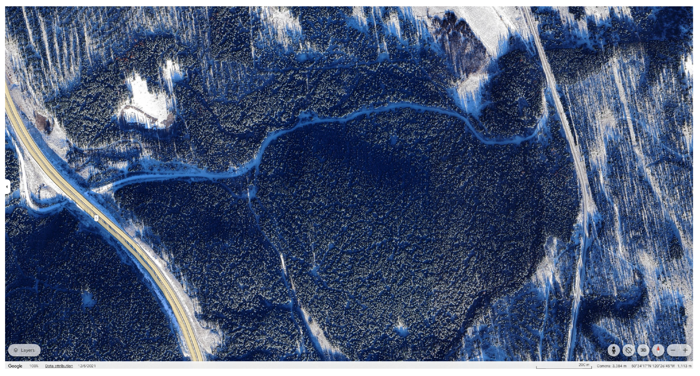
Figure 2.
The sample image view (top) and sample tree of Fir, Pine, Spruce, Aspen (bottom left to right).
Figure 2.
The sample image view (top) and sample tree of Fir, Pine, Spruce, Aspen (bottom left to right).
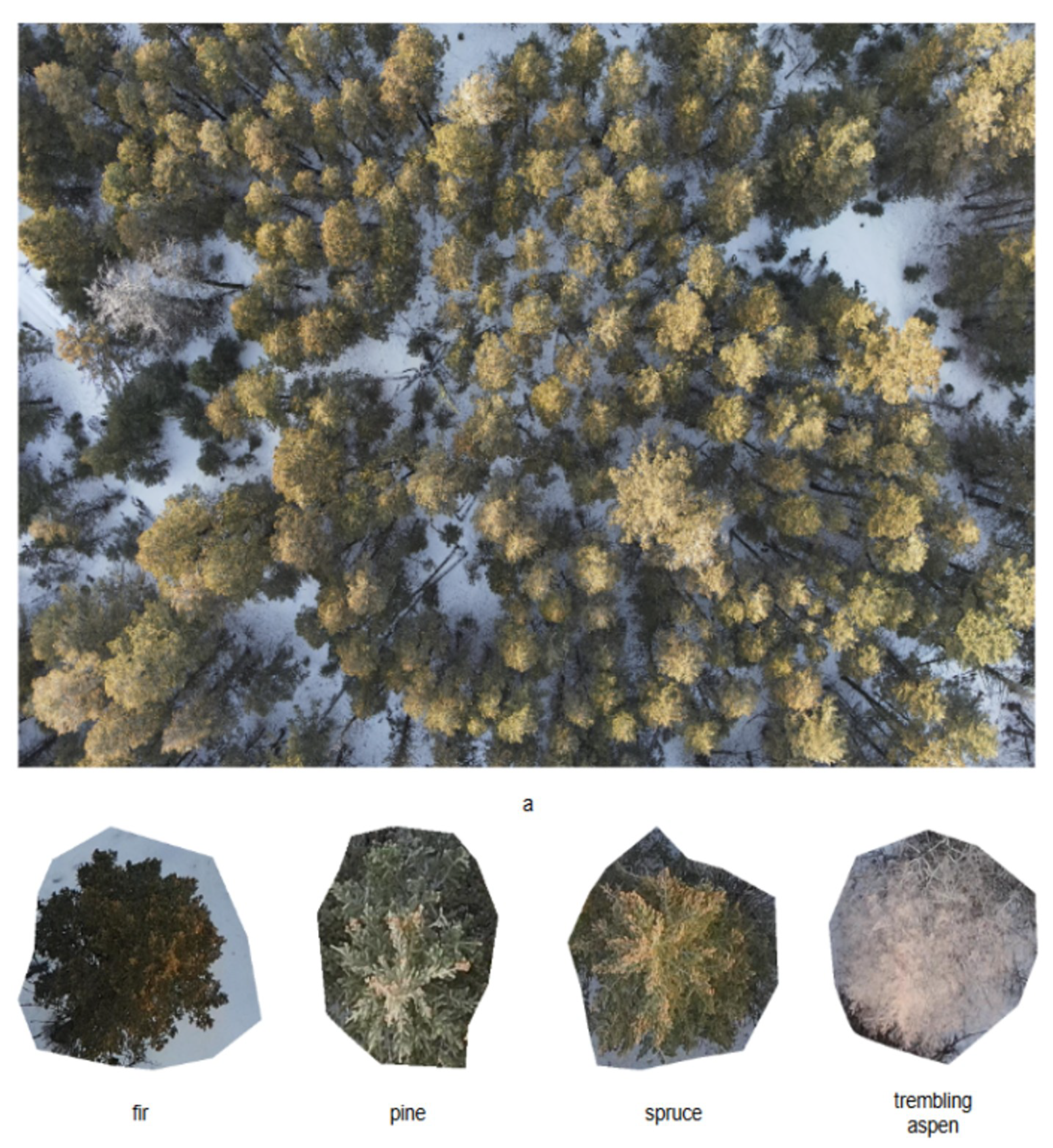
Figure 3.
The PTC generation workflow
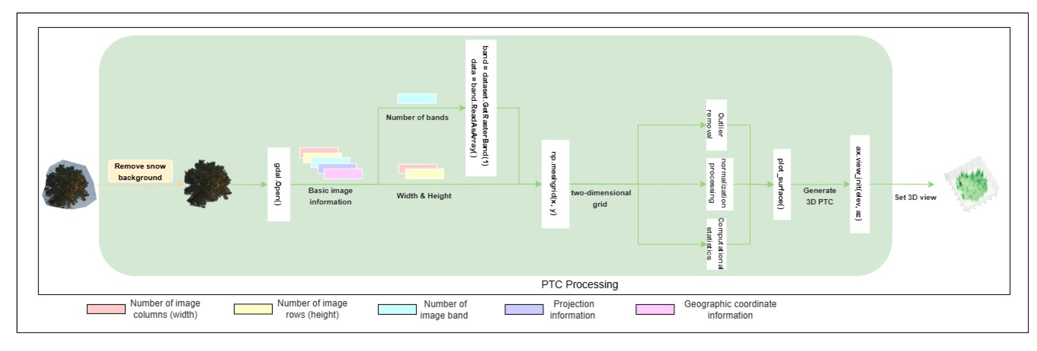
Figure 4.
The sample of pre-processing of background snow removal. (a) Fir (b) Pine (c) Spruce (d) Aspen
Figure 4.
The sample of pre-processing of background snow removal. (a) Fir (b) Pine (c) Spruce (d) Aspen
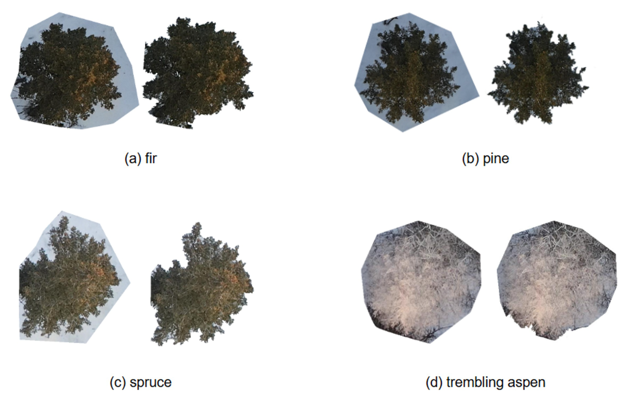
Figure 5.
The sample of PTC with snow background removed
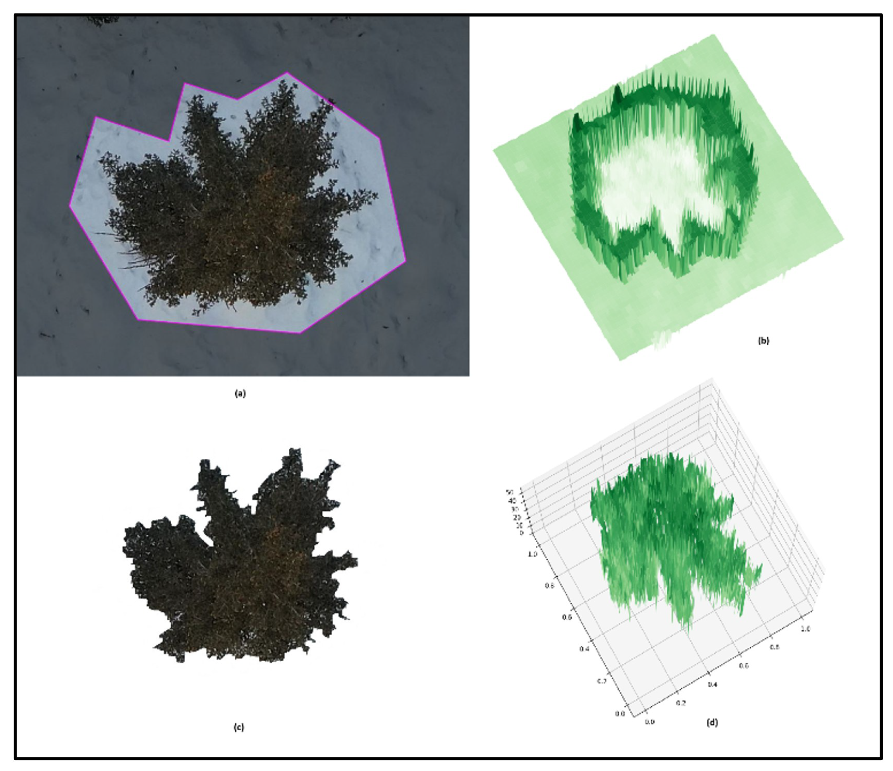
Figure 6.
The PTC in RF classifier workflow
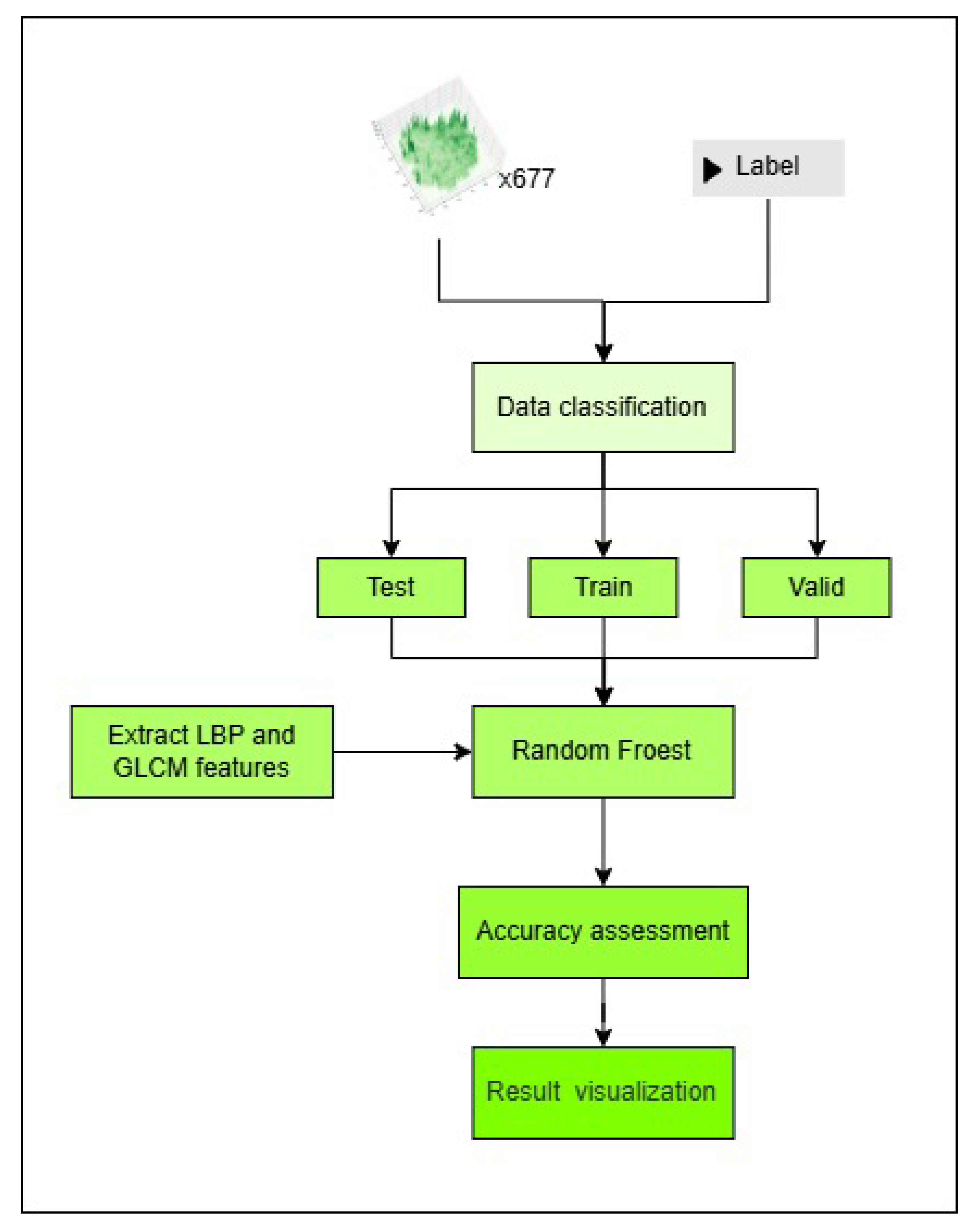
Figure 7.
The PTC in PyTorch (ResNet50) classifier workflow
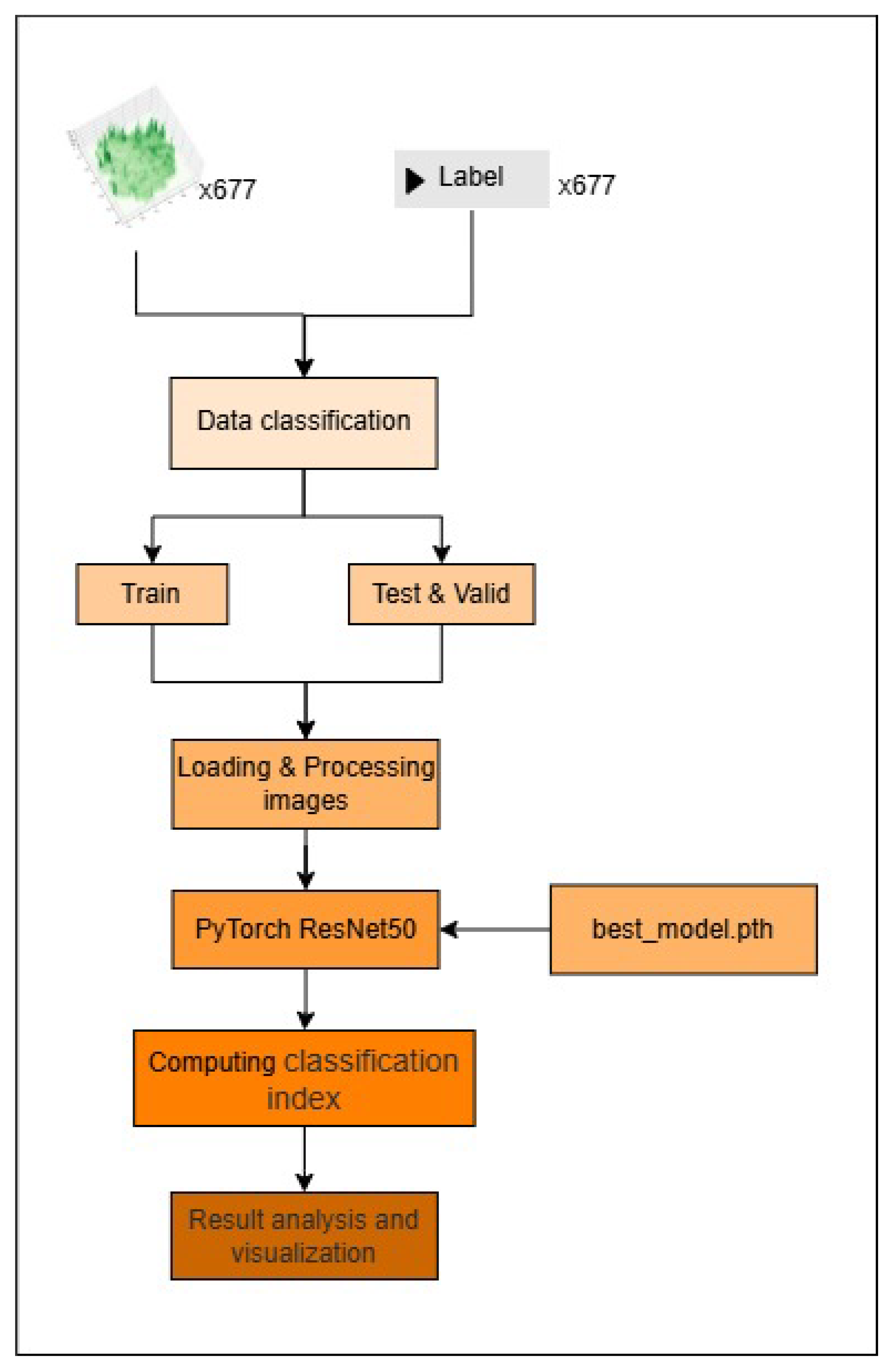
Figure 8.
The PTC in YOLO (v10, v11 and v12) classifier workflow
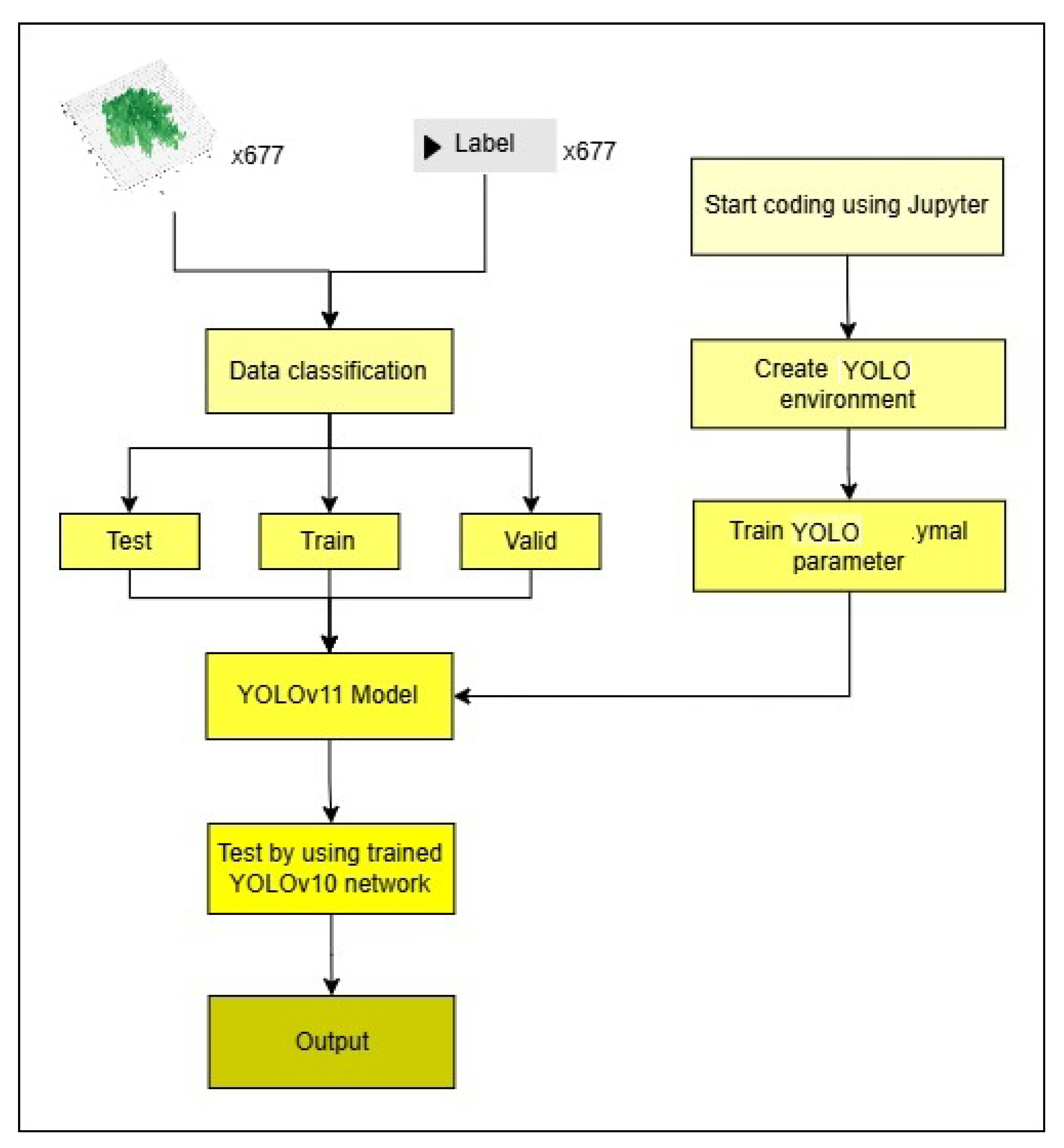
Figure 9.
The confusion matrix of RGB (left) and PTC (right) classification using RF
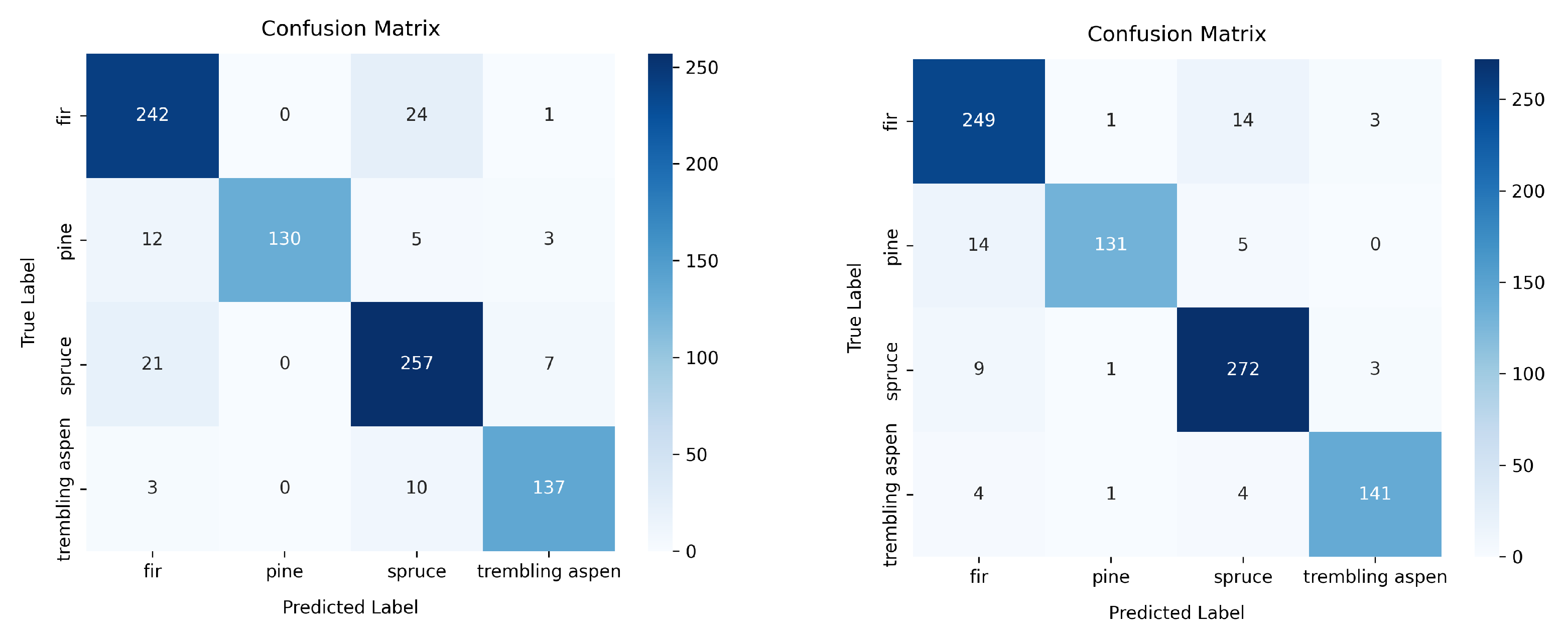
Figure 10.
The confusion matrix of RGB (left) and PTC (right) classification using PyTorch (ResNet50)
Figure 10.
The confusion matrix of RGB (left) and PTC (right) classification using PyTorch (ResNet50)
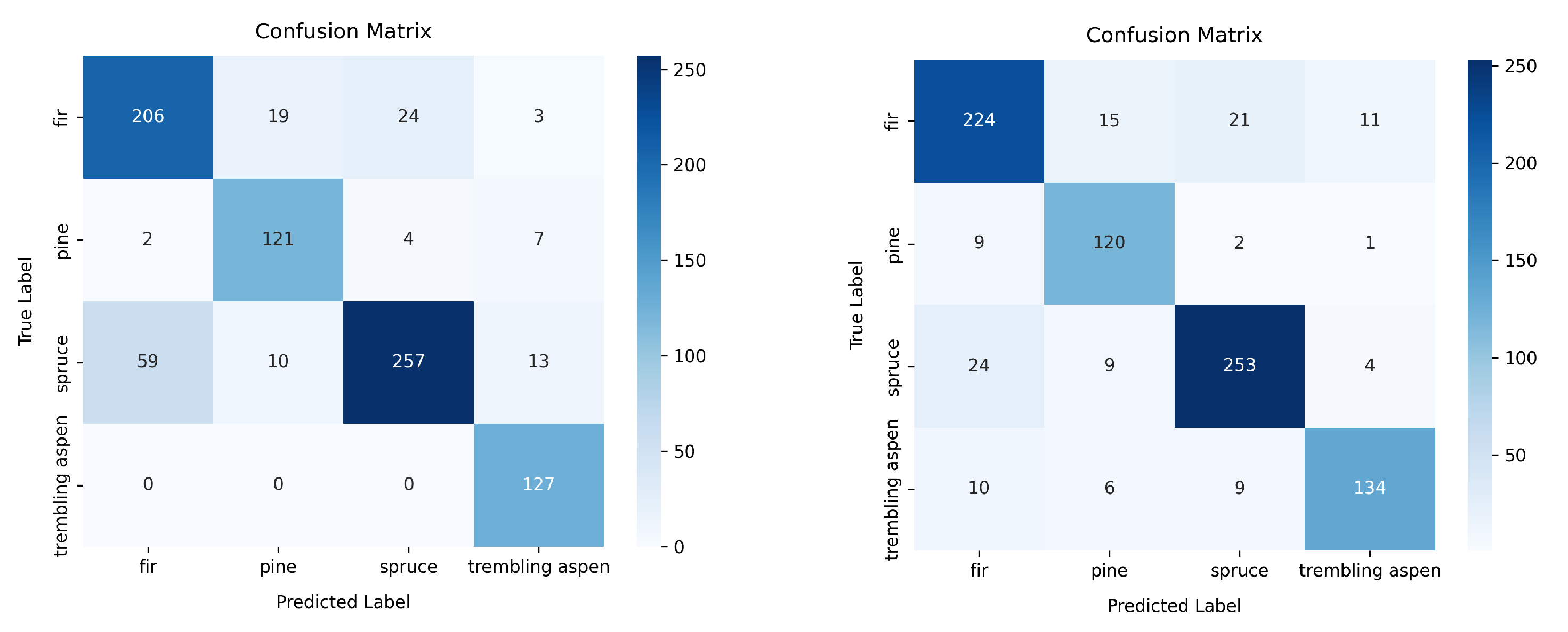
Figure 11.
The confusion matrix of RGB (left) and PTC (right) classification using YOLOv10
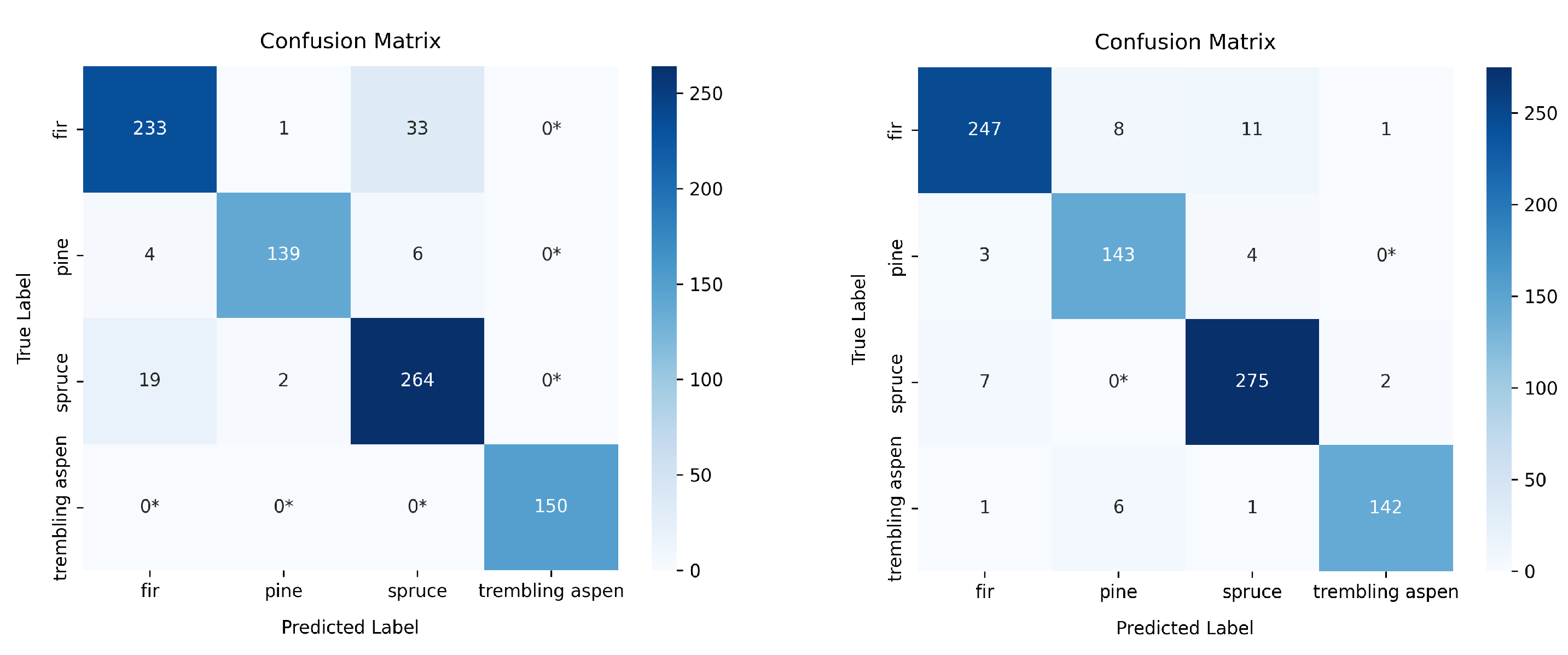
Figure 12.
The confusion matrix of RGB (left) and PTC (right) classification using YOLOv11
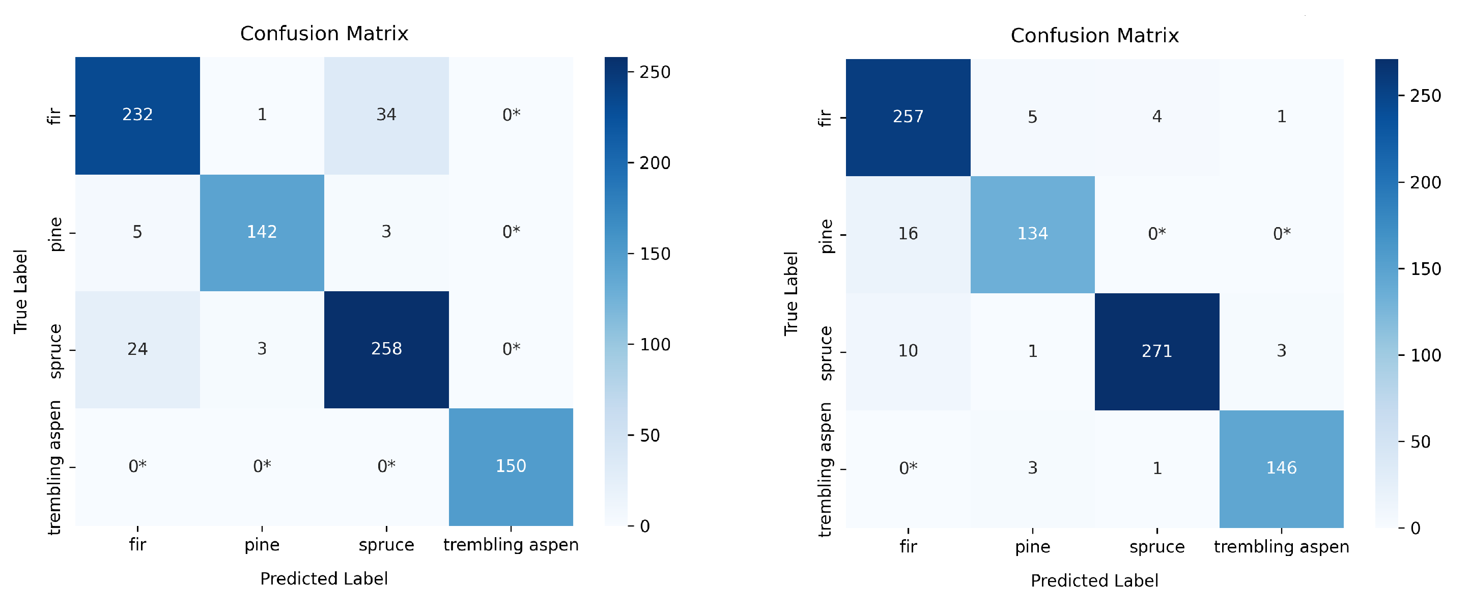
Figure 13.
The confusion matrix of RGB (left) and PTC (right) classification using YOLOv12
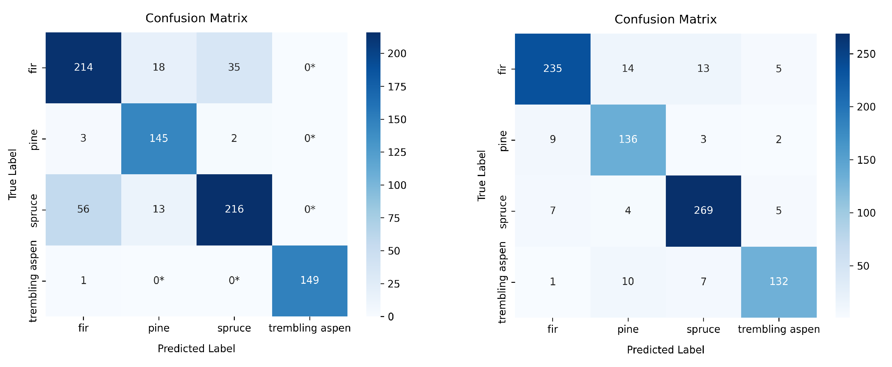

Table 1.
PyTorch (ResNet50) parameters
| Level | Layer Name | Input Channels | Output Channels | Kernel Size | Stride | Padding | Repetitions |
|---|---|---|---|---|---|---|---|
| Conv1 (Stage 0) | Conv | 3 | 64 | 7×7 | 2 | 3 | 1 |
| MaxPool1 | MaxPool | 64 | 64 | 3×3 | 2 | 1 | 1 |
| Stage1 | Bottleneck | 64 | 256 | 1×1 → 3×3 → 1×1 | (1,1,1) | (0,1,0) | 3 |
| Stage2 | Bottleneck | 256 | 512 | 1×1 → 3×3 → 1×1 | (2,1,1) | (0,1,0) | 4 |
| Stage3 | Bottleneck | 512 | 1024 | 1×1 → 3×3 → 1×1 | (2,1,1) | (0,1,0) | 6 |
| Stage4 | Bottleneck | 1024 | 2048 | 1×1 → 3×3 → 1×1 | (2,1,1) | (0,1,0) | 3 |
| AvgPool1 | AvgPool | 2048 | 2048 | – | – | – | 1 |
| FC Layer1 | Fully Connected | 2048 | 64 | – | – | – | 1 |
| FC Layer2 | Fully Connected | 64 | 4 | – | – | – | 1 |
Table 2.
The classification accuracy results with different models
| Model | RGB [%] | PTC [%] |
|---|---|---|
| RF | 89.9 | |
| PyTorch (ResNet50) | 83.4 | |
| YOLOv10 | 84.2 | |
| YOLOv11 | 83.3 | |
| YOLOv12 | 70.1 |
Table 3.
The classification results using Random Forest (RF)
| Data | Tree Species | Precision | Recall | F1-score | IoU |
|---|---|---|---|---|---|
| RGB | Fir | 0.8705 | 0.9064 | 0.8881 | 0.7987 |
| Pine | 1.0000 | 0.8667 | 0.9286 | 0.8667 | |
| Spruce | 0.8682 | 0.9018 | 0.8847 | 0.7932 | |
| Trembling aspen | 0.9257 | 0.9133 | 0.9195 | 0.8509 | |
| PTC | Fir | 0.9022 | 0.9326 | 0.9171 | 0.8469 |
| Pine | 0.9776 | 0.8733 | 0.9225 | 0.8562 | |
| Spruce | 0.9220 | 0.9544 | 0.9379 | 0.8831 | |
| Trembling aspen | 0.9592 | 0.9400 | 0.9495 | 0.9038 |
Table 4.
The classification results using PyTorch (ResNet50)
| Data | Tree Species | Precision | Recall | F1-score | IoU |
|---|---|---|---|---|---|
| RGB | Fir | 0.7715 | 0.8175 | 0.7938 | 0.6581 |
| Pine | 0.8067 | 0.9030 | 0.8521 | 0.7423 | |
| Spruce | 0.9018 | 0.7581 | 0.8237 | 0.7003 | |
| Trembling aspen | 0.8467 | 1.0000 | 0.9170 | 0.8467 | |
| PTC | Fir | 0.8390 | 0.8266 | 0.8327 | 0.7134 |
| Pine | 0.8000 | 0.9091 | 0.8511 | 0.7407 | |
| Spruce | 0.8877 | 0.8724 | 0.8800 | 0.7857 | |
| Trembling aspen | 0.8933 | 0.8428 | 0.8673 | 0.7657 |
Table 5.
The classification results using YOLOv10
| Data | Tree Species | Precision | Recall | F1-score | IoU |
|---|---|---|---|---|---|
| RGB | Fir | 0.9102 | 0.8727 | 0.8910 | 0.8034 |
| Pine | 0.9789 | 0.9329 | 0.9533 | 0.9145 | |
| Spruce | 0.8713 | 0.9263 | 0.8980 | 0.8148 | |
| Trembling aspen | 1.0000 | 1.0000 | 1.0000 | 1.0000 | |
| PTC | Fir | 0.9574 | 0.9251 | 0.9410 | 0.8885 |
| Pine | 0.9108 | 0.9533 | 0.9316 | 0.8720 | |
| Spruce | 0.9450 | 0.9683 | 0.9565 | 0.9167 | |
| Trembling aspen | 0.9793 | 0.9467 | 0.9627 | 0.9281 |
Table 6.
The classification results using YOLOv11
| Data | Tree Species | Precision | Recall | F1-score | IoU |
|---|---|---|---|---|---|
| RGB | Fir | 0.8889 | 0.8689 | 0.8788 | 0.7838 |
| Pine | 0.9726 | 0.9467 | 0.9595 | 0.9221 | |
| Spruce | 0.8746 | 0.9053 | 0.8897 | 0.8012 | |
| Trembling aspen | 1.0000 | 1.0000 | 1.0000 | 1.0000 | |
| PTC | Fir | 0.9081 | 0.9625 | 0.9345 | 0.8771 |
| Pine | 0.9371 | 0.8933 | 0.9147 | 0.8428 | |
| Spruce | 0.9819 | 0.9509 | 0.9661 | 0.9345 | |
| Trembling aspen | 0.9733 | 0.9733 | 0.9733 | 0.9481 |
Table 7.
The classification results using YOLOv12
| Data | Tree Species | Precision | Recall | F1-score | IoU |
|---|---|---|---|---|---|
| RGB | Fir | 0.7810 | 0.8015 | 0.7911 | 0.6544 |
| Pine | 0.8239 | 0.9667 | 0.8896 | 0.8011 | |
| Spruce | 0.8538 | 0.7579 | 0.8030 | 0.6708 | |
| Trembling aspen | 1.0000 | 0.9933 | 0.9967 | 0.9933 | |
| PTC | Fir | 0.9325 | 0.8801 | 0.9056 | 0.8275 |
| Pine | 0.8293 | 0.9067 | 0.8662 | 0.7640 | |
| Spruce | 0.9212 | 0.9439 | 0.9324 | 0.8734 | |
| Trembling aspen | 0.9167 | 0.8800 | 0.8980 | 0.8148 |
Table 8.
The classification results with and without snow background
| Data | YOLO | with | without |
|---|---|---|---|
| RGB | v10 | 0.8498 | 0.9236 |
| v11 | 0.8330 | 0.9178 | |
| v12 | 0.7010 | 0.8498 | |
| PTC | v10 | 0.9010 | 0.9483 |
| v11 | 0.8810 | 0.9484 | |
| v12 | 0.8310 | 0.9061 |
Table 9.
Comparison of RGB and PTC accuracy with different data set sizes: PyTorch (ResNet50)
| Dataset Size | RGB [%] | PTC [%] |
|---|---|---|
| 170 | 73.2 | 70.8 |
| 270 | 76.1 | 79.9 |
| 370 | 75.5 | 81.5 |
| 470 | 78.0 | 83.8 |
| 570 | 81.2 | 85.0 |
| 852 | 83.5 | 85.8 |
Table 10.
Comparison of RGB and PTC accuracy with different data set sizes: RF
| Dataset Size | RGB [%] | PTC [%] |
|---|---|---|
| 170 | 67.6 | 75.9 |
| 270 | 79.6 | 84.8 |
| 370 | 85.1 | 88.9 |
| 470 | 88.3 | 91.3 |
| 570 | 90.4 | 92.8 |
| 852 | 89.9 | 93.1 |
Table 11.
Comparison of RGB and PTC accuracy with different data set sizes: YOLOv10
| Dataset Size | RGB [%] | PTC [%] |
|---|---|---|
| 170 | 76.9 | 86.7 |
| 270 | 80.1 | 88.0 |
| 370 | 80.3 | 89.0 |
| 470 | 80.9 | 90.7 |
| 570 | 83.4 | 91.9 |
| 852 | 84.2 | 90.1 |
Table 12.
Comparison of RGB and PTC accuracy with different data set sizes: YOLOv11
| Dataset Size | RGB [%] | PTC [%] |
|---|---|---|
| 170 | 73.2 | 83.5 |
| 270 | 78.0 | 81.8 |
| 370 | 79.0 | 82.7 |
| 470 | 81.1 | 85.8 |
| 570 | 82.9 | 88.1 |
| 852 | 83.3 | 88.1 |
Table 13.
Comparison of RGB and PTC accuracy with different data set sizes: YOLOv12
| Dataset Size | RGB [%] | PTC [%] |
|---|---|---|
| 170 | 66.8 | 79.7 |
| 270 | 70.3 | 77.7 |
| 370 | 67.2 | 79.5 |
| 470 | 69.1 | 81.3 |
| 570 | 70.9 | 83.4 |
| 852 | 70.1 | 81.3 |
Disclaimer/Publisher’s Note: The statements, opinions and data contained in all publications are solely those of the individual author(s) and contributor(s) and not of MDPI and/or the editor(s). MDPI and/or the editor(s) disclaim responsibility for any injury to people or property resulting from any ideas, methods, instructions or products referred to in the content. |
© 2025 by the authors. Licensee MDPI, Basel, Switzerland. This article is an open access article distributed under the terms and conditions of the Creative Commons Attribution (CC BY) license (http://creativecommons.org/licenses/by/4.0/).
Copyright: This open access article is published under a Creative Commons CC BY 4.0 license, which permit the free download, distribution, and reuse, provided that the author and preprint are cited in any reuse.


