
Submitted:
28 July 2025
Posted:
29 July 2025
You are already at the latest version
Abstract
Process designs based on deterministic simulations without considering parameter uncertainty or variability have a high probability of not meeting specifications. Here, uncertainty and global sensitivity analysis are applied to a biogas upgrading membrane process implemented in the COCO process simulator for a controlled and a non-controlled scenario. This process required implementing a user model code to simulate gas separation membrane stages and performing a previous study of the membrane parameter uncertainty. A unit to generate combinations of uncertainty factors was developed to interact with the parametric tool of the simulator to evaluate the factor combinations. Morris' global sensitivity analysis was applied to the generated results to compare the importance of feed variability and membrane parameter uncertainty on the uncertainty of the product streams and process utilities. It was obtained that feed flow and composition variability greater than ±10% predominated over the membrane parameter uncertainty. Uncertainty analysis using the Montecarlo propagation method yielded the lower and upper tolerance limits of the main responses for a given probability content. The results showed substantial differences in the relative range tolerance for different responses and scenarios.
Keywords:
Uncertainty
; Global sensitivity
; Biogas upgrading
; Methane
; Carbon dioxide
; COCO simulator
; Simulatio
1. Introduction
1.1. Uncertainty and Global Sensitivity Analysis
In chemical engineering, modelling and simulation allow for studying process performance. Process simulators are helpful for process design because they can rapidly assess different process configurations and operating parameters.
It should be noted that process simulators provide a deterministic solution. However, in real processes, some parameters of the process units are not known with precision. Similarly, the feed characteristics and the influencing environment are subjected to variations. The uncertainty of these factors introduces, in turn, uncertainty in the process response, leading to a mismatch with the simulator results. Because numerical predictions are often the basis of engineering decisions, uncertainty quantification is a subject of concern [1]. Uncertainty analysis allows for quantifying the impact of the variability of factors on process outcomes, enabling the determination of potential limits for the process response. This allows for the robustness and confidence of the simulation results to be assessed. Many process simulators allow parametric sensitivity studies where one or several parameters can be modified to study their effect on critical process outcomes. However, a further step can be taken by applying global sensitivity analysis to know how the uncertainty in the output of a model can be apportioned to different sources of uncertainty in the model input [2]. Thus, this technique can answer which of the uncertain input factors are more critical in determining the uncertainty in the outputs of interest.
1.2. CAPE-OPEN Process Simulators
Process simulators combine physical properties databases, thermodynamic models, unit operation models, and numerical solvers with the capability to develop flowsheets in which model units are connected to form a process. As the best modelling options may come from different sources, many researchers point out the advantages of using CAPE-OPEN standards for their integration. These standards facilitate the implementation of new unit operations in different coding software. This can be crucial for particular unit operations like membrane stages. The simulator chosen for this study, the COCO simulator, offers excellent flexibility for this purpose. This simulator presents the advantages of being a free-of-charge CAPE-OPEN compliant steady-state simulation environment that demonstrates strong reliability in performing material and energy balances, with results closely aligned with those obtained from commercial process simulators [3]. The software allows interaction with user unit operations through add-ons developed by the COCO developer [4]. These units can be implemented in Excel, MATLAB, or free numerical software like Scilab and Python [5].
1.3. Scope of This Work
This work aims to demonstrate the applicability of global uncertainty and sensitivity analysis using the COCO simulator. For this purpose, a biogas upgrading process was chosen. The increasing interest in biomethane as a substitute for natural gas has led to the development of biogas upgrading techniques. Among these technologies, gas permeation based on membranes stands out. In recent years, the development efforts for these processes have focused on the design and analysis of stage configurations with the aim of energetic and economic optimization [6,7,8,9]. We have not found studies addressing the global sensitivity and uncertainty of this specific case. However, some studies deal with local sensitivity through parameter variation [10,11,12]. In these cases, the procedures used were aimed at optimization. In contrast, in our case, global sensitivity was applied to study the uncertainty and global sensitivity of the responses of an optimized system.
This work is structured in the following steps: i) A case definition based on an optimized CO2/CH4 separation process existing in the literature. ii) The development of the deterministic model of the process in the COCO simulator, adding a user unit to model gas membrane stages. iii) Identifying and characterizing the uncertainty factors through a bibliographic study. iv) Preparing the process model to accept uncertainty inputs and generating model results for specified input combinations. v) The subsequent uncertainty and global sensitivity analysis and their posterior interpretation.
2. Materials and Methods
2.1. Case Study
To demonstrate the application of uncertainty calculations using the COCO simulator to a biogas-upgrading process, we defined a case study based on the process configuration developed by Evonik [13]. This process was intended to obtain high gas purities using a three-membrane stage configuration with recirculation using a single compressor. Figure 1 shows the process flowsheet implemented in the simulator. In the process, two membrane stages are placed in series; the permeate of the first stage is sent to the third stage, and the permeate stream of the third stage, after decompression, is mixed with the permeate of the second stage to form a stream that is recirculated to be mixed with the process feed. Structural optimization for this process was performed in a thesis [14] for a biogas feed composed of 40% CO2 and 60% CH4 upgraded using a typical polyimide membrane with a CO2 permeance of 60 GPU, obtaining optimal stage areas and pressure for the permeate stream from stage 1 feeding stage 3 (Table 1).
For this study, we considered two operating scenarios for the same process configuration: (i) with active control of the compressor pressure to achieve a constant CH4 mole fraction of 0.96 in the biomethane product, and (ii) without pressure control. The mole fraction set point of the first scenario was chosen to be very close to the output obtained for the second scenario at the reference values. These scenarios were compared regarding their sensitivity to input uncertainties and process variability. The setpoint of composition for the scenario with regulation was chosen to be close to that obtained for the reference parameters in the unregulated system.
2.2. Deterministic Simulation of the Process in COCO
The deterministic simulation of the case study was performed before the uncertainty analysis, considering the parameters of Table 1 as deterministic. The process model was developed using the COCO simulator (version 3.9.0.1). The thermodynamic model for the whole process was based on the Peng-Robinson equation of state, which is commonly used in modelling membrane gas separation, and which handles non-ideal behavior of CO2 reasonably well [15].
Figure 1 shows the flow diagram of the case study implemented in the simulator’s flowsheet environment (COFE). The feed process (BG) is separated into an upgraded biomethane stream (BM) and an off-gas stream (OG), rich in carbon dioxide. The stage membranes (units MB1, MB2, and MB3) used the reference parameter values from Table 1. The compressor CP, placed after mixing the feed and recirculation, was assigned an isentropic efficiency of 72%. An aftercooler HX was set to reduce the temperature of the feed of the membrane stage MB1 to 40 ℃. The output pressure of the valve after the retentate of MB1 was set at the same pressure as the permeate of MB2 (1 bar).
The process simulator included some predefined units needed: compressor, heat exchanger, valve, and mixer units. Still, it does not include a membrane gas separation stage. The code for this unit operation was implemented in MATLAB and connected to the add-on “MATLAB unit operation” developed by Amsterchem [4] to define a user unit of a membrane gas separation stage able to communicate with the COCO environment. The equations used to create this user unit can be found in Appendix A. This subroutine was included as an additional user MATLAB unit operation file. The MATLAB unit operation also required an interface to receive the default stage parameters (stage area, component permeances, and permeate pressure). Ports were also added for the input and output streams of the stage. Additional ports for information were also included. These ports were a key component for the uncertainty analysis, as they allowed modifying the default parameters of the unit according to the information sent from an uncertainty generation unit.
Note that Figure 1 includes the control of the compressor output pressure to fix the methane product composition using the information streams xCH4 y Pout (not active in the unregulated scenario).
2.3. Application of Uncertainty and Sensitivity Methodology
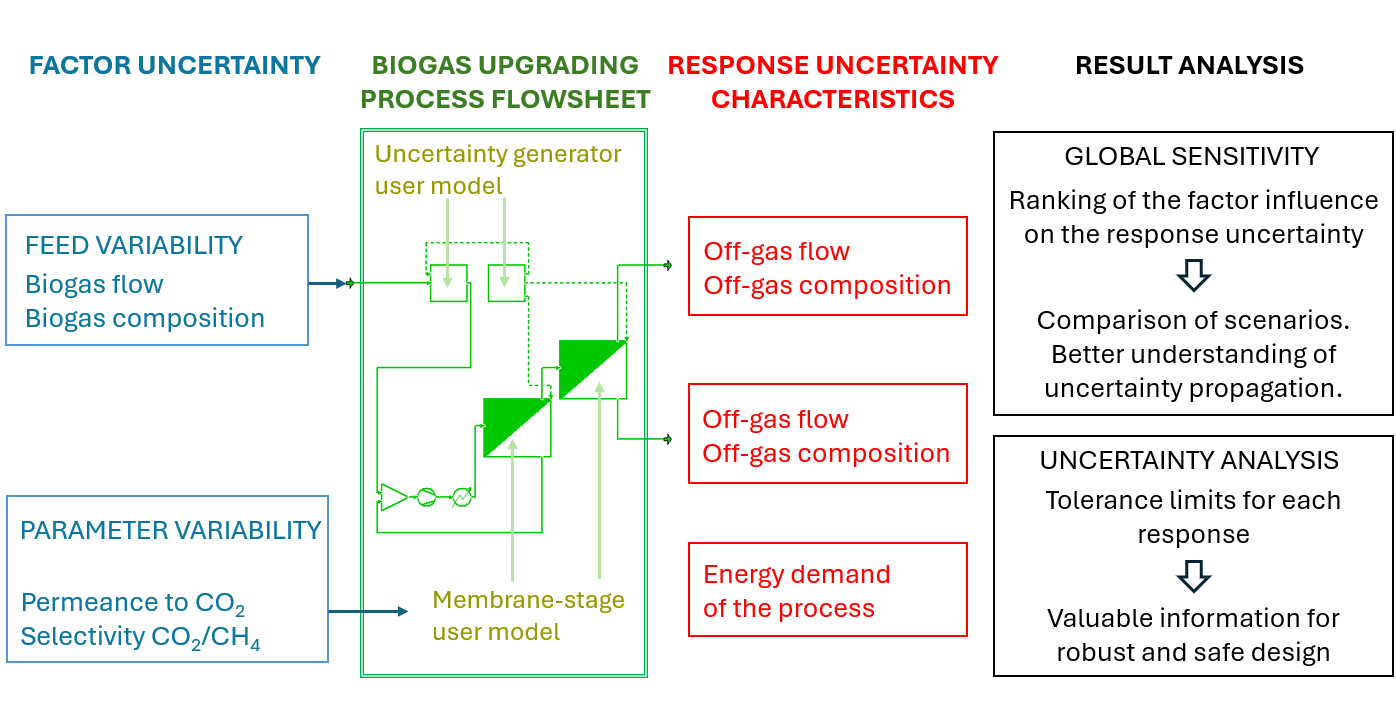
Uncertainty and sensitivity analyses require characterizing the uncertainty of the most essential uncontrollable factors in the process. Appropriate ranges of variation must be determined, and probability density distribution functions must be proposed, with statistical parameters to be fitted. The uncertainty distributions of the factors were used to perform a global sensitivity analysis with the Morris method to rank the importance of the factors. The uncertainty analysis was also applied to determine the uncertainty expected for the product flow and composition and the compression energy requirements.
2.3.1. Characterization of the Uncertainty Sources
Feed variability can be significant in terms of flow and composition. When periodical measurements are available, an empirical distribution can be obtained for the flow rate, but typically, global sensitivity methods use log-normal, normal (truncated to zero), or uniform distributions. The choice between these options depends on the approximate knowledge of the empirical distribution. However, for an exploratory sensitivity study, a uniform distribution can be appropriate when a range can be defined, if we want to avoid introducing unsupported assumptions. As we are interested in studying the effect of variability, we will use uncertainty ranges of flow at two levels of variation, ±5% and ±10%, with respect to the reference value of the study. In the real system, the magnitude of the fluctuations will depend on the size of the gas holder tank placed before the membrane upgrading system.
As regards the variability of composition, some general ranges can be found in the literature. Guerrero et al. found that in biogas obtained from anaerobic digestion of biomass, the methane range can be 35-85%, and the carbon dioxide range 10-65%, the rest of the components being much less significant [16]. The type and mixture of the feedstocks, operating conditions, and temporal fluctuations cause the variability observed [17,18]. Our reference feed values fall inside the mentioned ranges. However, to assume the wide ranges shown as uncertainty ranges in the plant design may not be realistic, as a plant is fed with a restricted class of organic sources. In our case, only the uncertainty range for CO2 molar fraction was used as a factor, as the analysis did not consider minor biogas components. Consequently, the CH4 molar fraction is entirely dependent. Like in the flow analysis, for the CO2 molar fraction, a uniform distribution will be used at two levels of variation, ±5% and ±10%, with respect to the reference value of the study, which falls inside the bounds previously commented.
Membrane performance is another great source of uncertainty in many processes. Permeability and selectivity of membranes for gas separation can be affected by compaction of the polymeric membrane due to pressure [19,20]. For example, CO2 permeability can be reduced by 10% to 20% with respect to its nominal value. Besides, variations in the performance of different batches of membrane fibers have been observed [21]. The same membrane design can vary significantly depending on the manufacturing scale or production batch. However, it must also be considered that in a membrane stage, there is more than one membrane module; this means that the uncertainty in the performance of the stage is smaller than that of a single module. Permeability of CO2 and CH4 generally increases with temperature, showing an Arrhenius behavior [22]. Permeability increases because the diffusion through the polymer increases as the temperature rises, and it dominates over the possible solubility decrease. However, for CH4, this effect is more critical than for CO2, resulting in a decline in CO2/CH4 selectivity. For example, for polyimide membrane samples, an increase in the operating temperature from 35 ℃ to 45 ℃ increased CO2 permeabilities between 7-12% but CO2/CH4 selectivity was reduced by 9-21% [23]. The temperature after the compressor plus cooling subsystem will have low variability, as a well-instrumented system can control the temperature of the stream between ±1 ℃. Therefore, the temperature variability of the membranes will be caused by the environment surrounding the membrane stages, and the magnitude of the variation will depend on the system’s insulation. Considering the ranges exposed for variability of CO2 permeability, either due to manufacturing or affected by temperature, we will use for this permeability a uniform distribution with a variation of ±10% with respect to the reference value of the study. Membrane permeability and selectivity are not independent variables, as there is a trade-off between them. Robeson found an upper limit with a potential relationship between the permeability of CO2 and the CO2/CH4 selectivity [24]. The fitting of this limit (Eq. 6) is a superior bound that relates both properties to the same material. We will use this expression to relate selectivity (SCO2/CH4) and permeability to CO2 (pmbCO2) using the study’s reference values, assuming a variability of ±5% with respect to the calculated selectivity value.
Based on this discussion, the uncertainty factors and their associated uncertainties used in the uncertainty and sensitivity study are summarized in Table 2. For the feed, the variability of the flow and composition will be studied jointly through two levels of variation (FV=±5% and FV= ±10%).
2.3.2. Response Variables Studied
The effects of the uncertainty were studied on the flow and composition of the biomethane product stream (BM) and off-gas (OG), as well as on the utilities of energy and heat duty of the compressor. Table 3 shows the response variables considered.
2.3.3. User Module for Uncertainties
Using the COCO simulator, it is possible to perform local sensitivity analysis in which one or more variables of the process (stream variables or unit parameters) can be modified to study the effect on product streams or the energy requirements of the process units. However, global sensitivity analysis requires performing calculations for combinations of variables following probability distributions. To address this issue, we created a MATLAB unit that transmits the combinations of factors with uncertainty to the simulator for calculation (unit UG of Figure 2). This unit uses the deterministic values of the problem as parameters when a case variable has a flag value equal to 0. A parametric study modifies the flag value from 1 to the number of executions required. When the flag value is 1, the values of all the factor combinations are loaded into the computer’s random-access memory from a comma-delimited file previously prepared in MATLAB using its statistical functions. The values for the subsequent factor combinations are sent through information streams to the process units. A MATLAB user unit was incorporated for the inlet stream to modify its flow and composition around the inlet stream reference values. Another MATLAB user unit was created to distribute the uncertain permselective parameters to the three process stages (information dividers ID1 and ID2).
2.3.4. Morris’ Analysis of Global Sensitivity
Morris’ global sensitivity analysis was applied to the two scenarios of the case study. This method can be used as a screening method to determine the relative importance of the factors by computing elementary effects from distinct perturbations.
Figure 3 shows the workflow diagram used to perform the analysis. The information on reference values and uncertainty ranges was processed by the subroutine “morris” of the package sensitivity (version 1.30.1) [25] of R (version 4.5.1) to generate a design matrix with the combinations of factors to be calculated. The COFE flowsheet of the process, including the MATLAB unit operations for uncertainty generation and distribution, permits COCO to perform a parametric study. The results of this parametric study were manually exported to a comma-delimited file. The file was processed with the design matrix, again calling the subroutine “morris” in R software to obtain the sensitivity analysis results.
The design was of type OAT (one-at-a-time) with r=30 trajectories to have a relatively dense sampling. The number of evaluations for the k=4 uncertainty factors was N=(r+1)×k=150, which was considered an acceptable computing cost. Using a grid jump of less than or equal to half of the number of levels is recommended, so we started with a typical number of 4 levels with a grid jump of 2. Still, after analysis of the design matrix, these values were increased to avoid repeated combinations.
It is important to note that the method was applied to normalized responses obtained by dividing each response by its reference value. The reference values of the responses were the deterministic values obtained for the reference values of the factors. This allows for better comparison of relative sensitivity across responses as sensitivity results are interpreted in terms of percent change of the response.
2.3.5. Uncertainty Analysis for Determination of Tolerance Limits
In addition to determining the importance of the uncertainty factors, assessing their effects on the probability distribution of the response variables is interesting. This information can be used to obtain tolerance values that capture a certain probability content. Specifically, we are interested in symmetric tolerance limits (two-sided limits) to cover a probability content of 95%, which is the usual standard when no safety issues are involved.
The Monte Carlo propagation method was used to estimate the probability distribution of the outputs. A design matrix was generated in MATLAB by combining factors with random values that follow a uniform distribution within the ranges of Table 2. These data were arranged in a comma-delimited file and processed similarly to the workflow shown in Figure 3, but using MATLAB as the analysis tool.
The number of computer evaluations to achieve a specific confidence level can be obtained using Wilks’ formula. Using rank 1 (tolerance limits placed in the first and last values of the ordered vector) is usually acceptable when the tolerance limits are not close to safety limits. However, according to Porter [26], a higher rank statistic gives a more accurate and precise answer, and the improvement obtained by increasing the rank from 1 to 2 is greater than that obtained by increasing from rank 2 to 3. Therefore, we used the formula considering rank 2, which means that the lower tolerance limit is defined by the value in the second position of the ordered vector of results, and the upper tolerance limit is the value in the last but one position. A confidence level of 99% requires performing 198 simulator evaluations (68 more than for rank 1).
3. Results
3.1. Deterministic Simulation Results
Table 4 shows the results obtained using the COCO simulator for the process configuration and the reference values in Table 1. Comparing the values of the flows of biomethane and off-gas for the non-controlled scenario with those obtained by Scholz [14], we observed differences of 0.12% and −0.16% for the same configuration and reference parameters. These minor differences are probably a consequence of the most elaborate model of the mentioned work in terms of the internal structure of the stage. However, compared with the variability posteriorly observed in the uncertainty study, they are small enough to validate the process model for capturing the uncertainty characteristics of the process.
3.2. Sensitivity Analysis
3.2.1. Refined Matrix Design
Using four levels with a grid jump of 2 yielded a design matrix with repeated combinations of factors. This is not desirable when evaluating a computer code, as redundant effects are obtained. Therefore, we increased to 8 levels and a grid jump of 4 for an experimental plan with no repetitions (Figure 4).
Using an Intel Core i9 at 3.50GHz, the computing time in the simulator for the 150 combinations to calculate was 5.91 min for the non-controlled scenario and 75.3 min for the controlled case.
3.2.2. Morris Sensitivity Analysis of the Flow and Composition of the Product Streams
The Morris sensitivity analysis provides three main indices: the mean of elementary effects (μ), the mean of the absolute values of the elementary effects (μ*), and the standard deviation of the elementary effects (σ). The μ* index is usually used over μ as it avoids the cancellation between positive and negative effects, and indicates, on average, how much the input changes the output. The σ index measures the nonlinearity, i.e., the interaction between effects; low σ values indicate that the effect is linear or additive, high σ values indicate interaction and nonlinearity. Parameters with low values of μ* and σ are unimportant. A diagonal (σ=μ*) is also included in the figures to identify if the effects tend to be predominantly linear (σ<<μ*) or nonlinear (σ>>μ*).
Figure 5 shows the analysis for the response of the biomethane product flow (FBM). Let us consider the non-controlled scenario at a feed variability FV = ±5. The effects of the membrane parameter uncertainty (given by factors PCO2 and S) are negligible because of their low μ* and σ values. The flow of biogas FBG is the dominant factor, strong and with a linear effect; the biogas composition xCO2BG is lower, but not negligible. Comparing this situation with that obtained at FV=±10%, we can see that μ* has almost doubled, and that σ has increased notably, which suggests non-linear effects and interaction with other variables. The situation is similar to that in the controlled scenario.
Figure 6 shows the analysis for the response of the off-gas product flow (FOG). Thanks to the normalization of this variable, we observed similar index values. The result of the analysis is very similar to that performed for the FBM variable, except that now the effect of the CO2 fraction in the feed becomes somewhat more important than the biogas flow.
Figure 7 shows the analysis for the response of the methane fraction in the biomethane product (xCH4BM) for a non-controlled scenario. This response was not analyzed in the controlled scenario because it is set to a fixed value. We can see that for low feed variability (FV=±5), the membrane parameter uncertainty predominates over the feed variability as the permeance factor PCO2 has the higher μ* value; however, the variability of the selectivity with respect to the value expected for each permeance is not significant. Nevertheless, for FV=±10, the effect of the flow of biogas becomes practically as important as that of the membrane permeance. The smaller μ* values currently observed in the analysis of the composition response compared to those observed for the flow responses do not imply less significant effects. Note now that they represent relative composition variations with respect to a composition fraction value close to unity.
Figure 8 shows the analysis for the response of the CO2 fraction in the off-gas (xCO2OG). The results for the non-controlled and controlled scenarios are very similar. Like in the case of the xCH4BM response, at FV= ±5% the effect of the CO2 membrane permeance is the most important. Similarly, at the higher feed variability of FV= ±10%, feed variability becomes as important as membrane permeance uncertainty.
3.2.3. Morris’ Analysis of the Process Utilities
Figure 9 shows the analysis for the EDC response. In all situations, the uncertainty of biogas flow is the most critical factor (higher μ*), doubling when the feed variability is doubled. For the controlled system, the non-linear effects are higher (higher σ).
An additional study was performed on the mechanical power ratio to the flow of processed biogas (EDC/FBG). In Figure 10, we can see that, compared with the EDC analysis, a large part of the effect of the variability due to FBG has been cancelled, and the μ* values are smaller. Now, we appreciate different behaviors for the non-controlled and the controlled scenarios. In the non-controlled scenario, the effects of all factors are similar; however, for the controlled scenario, the impact of the permeance of CO2 is higher than the effect of FBG at FV= ±5% but it takes on a comparable value at FV= ±10%.
Morris’ analysis results of the thermal load to be removed in the compressor (HDX and HDX/FBG) were virtually identical to those of the mechanical power (Supplementary Materials figures S1 and S2). This is logical since both variables depend almost exclusively on the flow through the compression system.
3.3. Determination of Tolerance Limits of the Responses
Table 5 shows the uncertainty analysis results to obtain the lower and upper tolerance limit values for a 95% probability content and a 99% confidence level (LTL and UTL). The approximate form of each distribution can be represented, but for the sake of concision, two coefficients, RLG and RUG, were created as the relative gaps between lower and upper tolerance limits and the mean value. The coefficient of variation (CV), defined as the ratio of the standard deviation to the mean, was also included.
The mean values obtained for all variables did not differ significantly from those obtained for the reference factors (Table 4). The coefficients RLG and RUG had similar values for most responses, implying high symmetry for most distributions. For these responses, we can see that CV is approximately half of the relative gap values because, for a normal distribution, twice the CV is approximately 95% of the probability content. The highest difference in RLG and RUG was found for the response xCH4BM under the non-controlled scenario, with RLG representing 59% of the total tolerance gap. A reason can be found in the fact that the values of this variable are near an upper physical bound, and the left tail of the distribution predominates. The values of relative tolerance gaps were much higher for the flows (FBM and FOG), and utility variables related to them through the recirculated flow (EDC and HDX). For these responses, doubling the feed variability approximately doubles the gap value. The tolerance gap and CV were smaller for the composition-related variables (xCH4BM and xCO2OG), and the impact on the tolerance gap of doubling the feed variability was smaller.
The controlled and non-controlled scenarios yield similar results for many variables, but differences were observed in some specific responses. The tolerance interval was null for the controlled variable xCH4BM, as it is a system property, but this fact did not substantially increase the tolerance gap for the response xCO2OG. However, the tolerance gaps for the ratios EDC/FBG and HDX/FBG are much higher for the controlled scenario because of the necessary regulation effort of the pressure to achieve the set point of methane composition in the biomethane product.
4. Discussion
This paper shows the feasibility of conducting sensitivity and uncertainty analysis of processes combining free tools such as the COCO simulator and R. However, it is still necessary to model some specific units using programming software like MATLAB or other free software. This analysis can be largely automated using parameterization and reading from bridge files.
Studies on uncertainty and sensitivity in areas related to our process, such as anaerobic digestion [27], or gas membrane plants [28,29], indicate the usefulness of Morris’ analysis as a screening method to rank the importance of the factors. In this way, factors with a low influence on the uncertainty of a response can be potentially fixed without affecting the prediction.
However, Morris’ analysis has limitations as it does not provide variance-based quantitative indices. Other global sensitivity methods, like Sobol or eFAST, are more robust and can be used in a second phase on a subset of the influential variables to get quantitative sensitivity indices and evaluate interactions. Nevertheless, it should be considered that these methods involve a high number of computing evaluations, and difficulties may arise when an evaluation fails in the calculation process.
In our case, we have seen that the effects of feed variability are most influential in the uncertainty of product flows and power and heat demand responses. However, for product composition, the parameter uncertainty of membrane permeance can be most influential when feed variability is under ±10%. The important effect observed of the flow and composition variability of the feed agrees with what has been determined using parameter variation in other studies in a biogas processing plant [11].
The uncertainty analysis yielded lower and upper tolerance limits to cover a probability content of 95%. A study about the life cycle assessment of a biomethane production recommends its use to test the robustness of the results [30]. According to [31], simplified models are likely to overpredict performance compared to experimental results; therefore, the uncertainty quantification can help quantify the estimates of uncertain designs. In conclusion, knowing the tolerance limits is beneficial information for process design. Let us suppose the obtained tolerance limits are bound to be unacceptable. In that case, we can modify the process (unit dimensions or structure) or the operating parameters and include additional control to ensure the correct functioning of the process. In our case, stream flow showed high variability, so the information of their probability distributions can be used to size the gas-holding tanks before the upgrading process. Seemingly, the lower tolerance limit of the power demand of the compressor could be used to specify its nominal power. For the composition of the product stream, smaller tolerance limits were obtained. However, modifications of the process, like increasing the membrane stage areas or system pressures, may be necessary if a tolerance limit is close to an undesirable value. One crucial observation must be considered when applying the uncertainty analysis procedure to a process. For simplicity, we have considered in the case study that the variability of feed flow rates is independent of the composition variability, which may not be the case in some real-life situations. As Porter [26] discussed, when there is a correlation between variables, the joint distribution should be propagated, since otherwise, the uncertainty is overpredicted.
For the case study, different uncertainty and sensitivity characteristics were obtained when comparing the controlled and non-controlled scenarios of the same system. Similar situations can happen for changes in the configuration or the relative size of the different process units. This encourages us to focus future studies on understanding how the process configuration influences the uncertainty of the outputs.
Supplementary Materials
The following supporting information can be downloaded at: Preprints.org, Figure S1: Morris’ results of the heat duty demand of the heat exchanger of the compressor system (HDX) for the non-controlled and controlled scenarios at two levels of feed variability (FV).; Figure S2: Morris’ results of the ratio of the heat duty demand of the heat exchanger to biogas flow (HDX/FBG) for the non-controlled and controlled scenarios at two levels of feed variability (FV).
Author Contributions
Conceptualization, J.M.G.Z.; methodology, J.M.G.Z. and A.S.M.; software, J.M.G.Z.; validation, J.M.G.Z. and A.S.M.; formal analysis, J.M.G.Z. and A.S.M..; investigation, J.M.G.Z.; resources, J.M.G.Z. and A.S.M.; data curation, J.M.G.Z. and A.S.M..; writing—original draft preparation, J.M.G.Z. and A.S.M..; writing—review and editing, J.M.G.Z and A.S.M.; visualization, J.M.G.Z.; supervision, J.M.G.Z.
Funding
This research received no external funding.
Data Availability Statement
The dataset used in the uncertainty analysis that was generated with the model can be accessed at https://doi.org/10.5281/zenodo.16084093
Acknowledgments
The authors gratefully acknowledge AmsterCHEM for providing access to the COCO simulator. Special thanks to Jasper van Baten and Richard Baur for their development and maintenance efforts that support ongoing educational and research applications. We also acknowledge the R Core Team for developing R for statistical analysis and the developers of the sensitivity R package (Ioss et al., 2024). While preparing this manuscript, the authors used Grammarly (v.1.2.176) to assist in proofreading and improving the manuscript’s clarity. The authors have reviewed and edited the output and take full responsibility for the content of this publication
Conflicts of Interest
The authors declare no conflicts of interest.
Abbreviations
The following abbreviations are used in this manuscript:
| CAPE | Computer Assisted Process Engineering |
| COCO | Cape-Open to Cape-Open compliant steady-state simulator environment |
| COFE | Cape-Open Flowsheet Environment |
| FV | Feed variability |
| LTL | Lower Tolerance Limit |
| ODE | Ordinary differential equation |
| RLG | Relative lower-bound gap |
| Sc. | Scenario |
| RUG | Relative upper-bound gap |
| UTL | Upper tolerance limit |
Appendix A
This appendix shows the equations and solution procedure to perform the model for the user unit used to model the membrane stages of the process.
Figure A1 represents a differential membrane element. According to it, the balance equation of a component i in the feed chamber is:
where Fi is the flow of component i in the feed chamber and Ji is the permeate flux.
Figure A1.
Component flows in a differential element of the gas separation membrane.
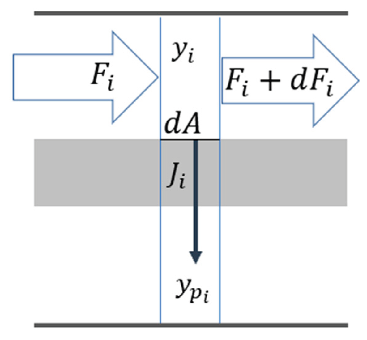
The permeate flux depends on the permeance of the component in the membrane, pmci, and the difference in partial pressure between the feed and permeate chambers.
The molar fraction in the feed of each component is related to the flows circulating in the feed chamber (Eq. A3). The permeate fraction of the component crossing the element of area is obtained from considering all permeate flows and neglecting mixing effects in the chamber (Eq. A4)
Equations (A3) and (A4), considered for all components, constitute equations that permit solving feed and permeate fractions. Using Eq. (A2), the component fluxes can be expressed as a function of the flows circulating along the feed chamber. Therefore, from Eq. (A1) and the knowledge of the permeate fluxes, the ODE set of Eq. (A5) can be integrated along the whole area of the module using the input feed composition as a contour condition.
References
- Soize, C. Uncertainty Quantification; 1st ed., Springer Cham, 2017; Vol. 23. [CrossRef]
- Saltelli, A.; Tarantola, S.; Campolongo, F.; Ratto, M. Global Sensitivity Analysis for Importance Assessment. In Sensitivity Analysis in Practice; Wiley, 2004; pp. 31–61. [CrossRef]
- Oyegoke, T. COCO, a Process Simulator: Methane Oxidation Simulation & Its Agreement with Commercial Simulator’s Predictions. 2023, 18, 995–1004. [CrossRef]
- Amsterchem COCO Cape Open to Cape Open Simulation Environment. https://www.amsterchem.com/coco.html. (accessed on 01/05/2025)2025.
- Alqaheem, Y.; Alobaid, M. Development of a Membrane Process in CAPE-OPEN to CAPE-OPEN (COCO) Simulator for Carbon Dioxide Separation. Results in Engineering 2024, 22. [Google Scholar] [CrossRef]
- Iarikov, D.D.; Ted Oyama, S. Review of CO2/CH4 Separation Membranes. Membrane Science and Technology 2011, 14, 91–115. [Google Scholar] [CrossRef]
- Tomczak, W.; Gryta, M.; Daniluk, M.; Żak, S. Biogas Upgrading Using a Single-Membrane System: A Review. Membranes (Basel) 2024, 14. [Google Scholar] [CrossRef]
- Janusz-Cygan, A.; Jaschik, J.; Tańczyk, M. Upgrading Biogas from Small Agricultural Sources into Biomethane by Membrane Separation. Membranes (Basel) 2021, 11. [Google Scholar] [CrossRef]
- Vrbová, V.; Ciahotný, K. Upgrading Biogas to Biomethane Using Membrane Separation. Energy & Fuels 2017, 31, 9393–9401. [Google Scholar] [CrossRef]
- Abejón, R.; Casado-Coterillo, C.; Garea, A. Techno-Economic Optimization of Multistage Membrane Processes with Innovative Hollow Fiber Modules for the Production of High-Purity CO2 and CH4 from Different Sources. Ind Eng Chem Res 2022, 61, 8149–8165. [Google Scholar] [CrossRef]
- Deng, L.; Hägg, M.B. Techno-Economic Evaluation of Biogas Upgrading Process Using CO2 Facilitated Transport Membrane. International Journal of Greenhouse Gas Control 2010, 4, 638–646. [Google Scholar] [CrossRef]
- Zito, P.F.; Brunetti, A.; Barbieri, G. Multi-Step Membrane Process for Biogas Upgrading. J Memb Sci 2022, 652, 120454. [Google Scholar] [CrossRef]
- Ungerank, M.; Baumgarten, G.; Priske, M.; Roegl, H. Process for Separation of Gases 2012. WO 2012/00727.
- Scholz, M. Membrane Based Biogas Upgrading Processes, Dissertation/. PhD Thesis, Aachen, Techn. Hochsch.: Aachen, 2013. [Google Scholar]
- Böttcher, N.; Taron, J.; Kolditz, O.; Liedl, R.; Park, C.-H. Comparison of Equations of State for Carbon Dioxide for Numerical Simulations. In Proceedings ModelCARE2011 held at Leipzig, Germany, in September 2011 (IAHS Publ, 2011; Vol. 355).
- Guerrero Piña, J.C.; Alpízar, D.; Murillo, P.; Carpio-Chaves, M.; Pereira-Reyes, R.; Vega-Baudrit, J.; Villarreal, C. Advances in Mixed-Matrix Membranes for Biorefining of Biogas from Anaerobic Digestion. Front Chem 2024, 12. [Google Scholar] [CrossRef] [PubMed]
- Weiland, P. Biogas Production: Current State and Perspectives. Appl Microbiol Biotechnol 2010, 85, 849–860. [Google Scholar] [CrossRef] [PubMed]
- Petersson, A.; Wellinger, A. Biogas Upgrading Technologies-Developments and Innovations. Technical report in IEA Bioenergy Task 37-Energy from Biogas and Landfill. https://task37.ieabioenergy.com/technical-reports/.
- Li, Y.; Chen, D.; He, X. Preparation and Characterization of Polyvinylalcohol/Polysulfone Composite Membranes for Enhanced CO2/N2 Separation. Polymers (Basel) 2023, 15. [Google Scholar] [CrossRef]
- Kadirkhan, F.; Sean, G.P.; Ismail, A.F.; Wan Mustapa, W.N.F.; Halim, M.H.M.; Kian, S.W.; Yean, Y.S. CO2 Plasticization Resistance Membrane for Natural Gas Sweetening Process: Defining Optimum Operating Conditions for Stable Operation. Polymers (Basel) 2022, 14. [Google Scholar] [CrossRef]
- Haider, S.; Lie, J.A.; Lindbråthen, A.; Hägg, M.B. Pilot–Scale Production of Carbon Hollow Fiber Membranes from Regenerated Cellulose Precursor-Part II: Carbonization Procedure. Membranes (Basel) 2018, 8. [Google Scholar] [CrossRef]
- Adewole, J.K.; Ahmad, A.L.; Ismail, S.; Leo, C.P. Current Challenges in Membrane Separation of CO2 from Natural Gas: A Review. International Journal of Greenhouse Gas Control 2013, 17, 46–65. [Google Scholar] [CrossRef]
- Ansaloni, L.; Minelli, M.; Baschetti, M.G.; Sarti, G.C. Effects of Thermal Treatment and Physical Aging on the Gas Transport Properties in Matrimid®. Oil and Gas Science and Technology - Rev. IFP Energies nouvelles 2015, 70, 367–379. [Google Scholar] [CrossRef]
- Robeson, L.M. The Upper Bound Revisited. J Memb Sci 2008, 320, 390–400. [Google Scholar] [CrossRef]
- Iooss, B.; Da Veiga, S.; Janon, A.; Pujol, G. Sensitivity: Global Sensitivity Analysis of Model Outputs and Importance Measures (R Package Version 1. 30.1). 2024. [Google Scholar] [CrossRef]
- Porter, N.W. Wilks’ Formula Applied to Computational Tools: A Practical Discussion and Verification. Ann Nucl Energy 2019, 133, 129–137. [Google Scholar] [CrossRef]
- Barahmand, Z.; Samarakoon, G. Sensitivity Analysis and Anaerobic Digestion Modeling: A Scoping Review. Fermentation 2022, 8. [Google Scholar] [CrossRef]
- Chu, Y.; He, X. Process Simulation and Cost Evaluation of Carbon Membranes for CO 2 Removal from High-Pressure Natural Gas. Membranes (Basel) 2018, 8. [Google Scholar] [CrossRef]
- Dehkordi, J.A.; Hosseini, S.S.; Kundu, P.K.; Tan, N.R. Mathematical Modeling of Natural Gas Separation Using Hollow Fiber Membrane Modules by Application of Finite Element Method through Statistical Analysis. 2016, 11, 11–15. [CrossRef]
- Florio, C.; Fiorentino, G.; Corcelli, F.; Ulgiati, S.; Dumontet, S.; Güsewell, J.; Eltrop, L. A Life Cycle Assessment of Biomethane Production from Waste Feedstock through Different Upgrading Technologies. Energies (Basel) 2019, 12. [Google Scholar] [CrossRef]
- Da Conceicao, M.; Nemetz, L.; Rivero, J.; Hornbostel, K.; Lipscomb, G. Gas Separation Membrane Module Modeling: A Comprehensive Review. Membranes (Basel) 2023, 13. [Google Scholar] [CrossRef] [PubMed]
Figure 1.
Flowsheet of the process created in COFE, the COCO simulator flowsheet environment.
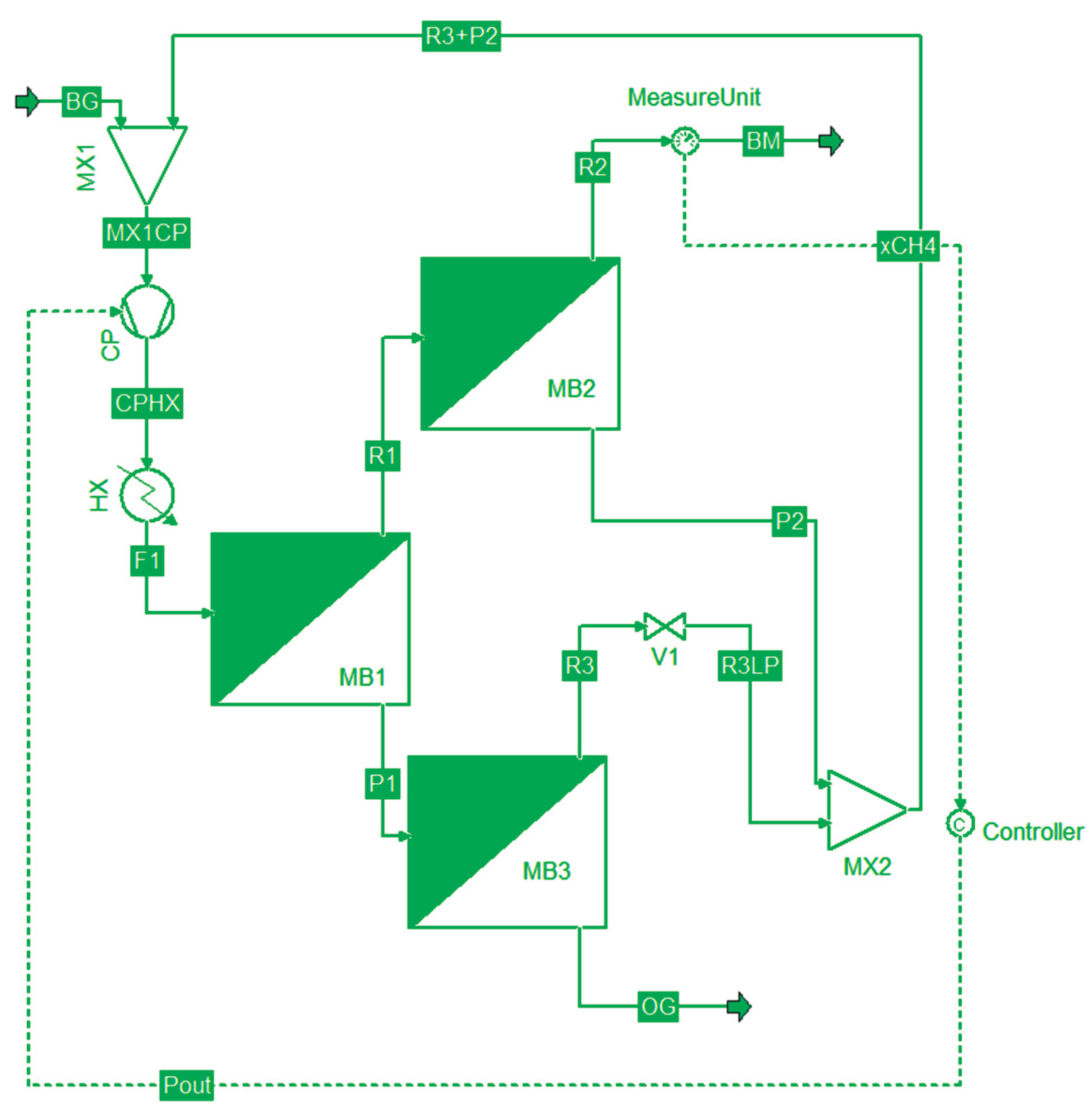
Figure 2.
COFE flowsheet including information streams for parameter perturbation.
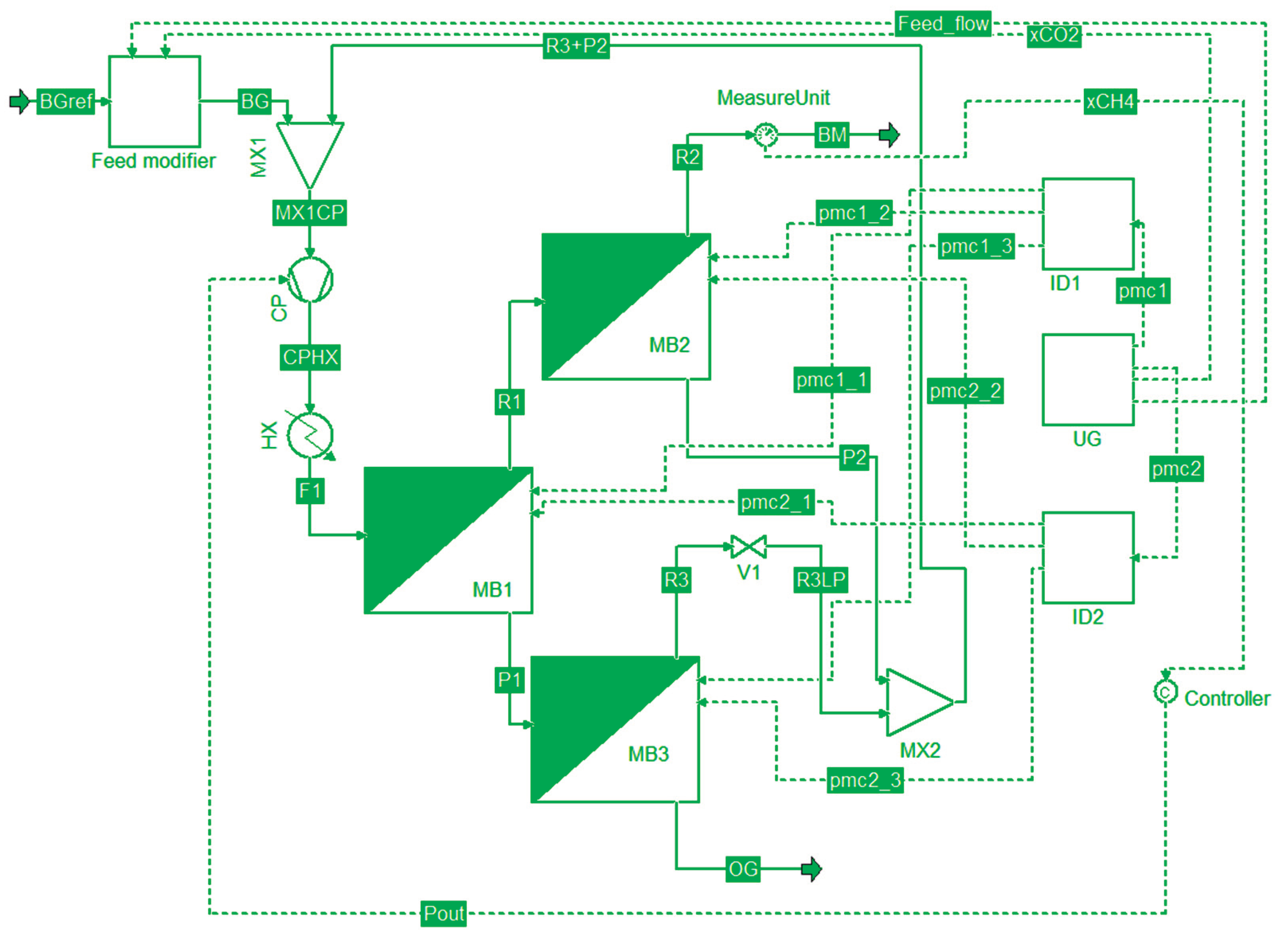
Figure 3.
Workflow diagram for sensitivity analysis using COCO simulator, MATLAB, and R environment.
Figure 3.
Workflow diagram for sensitivity analysis using COCO simulator, MATLAB, and R environment.
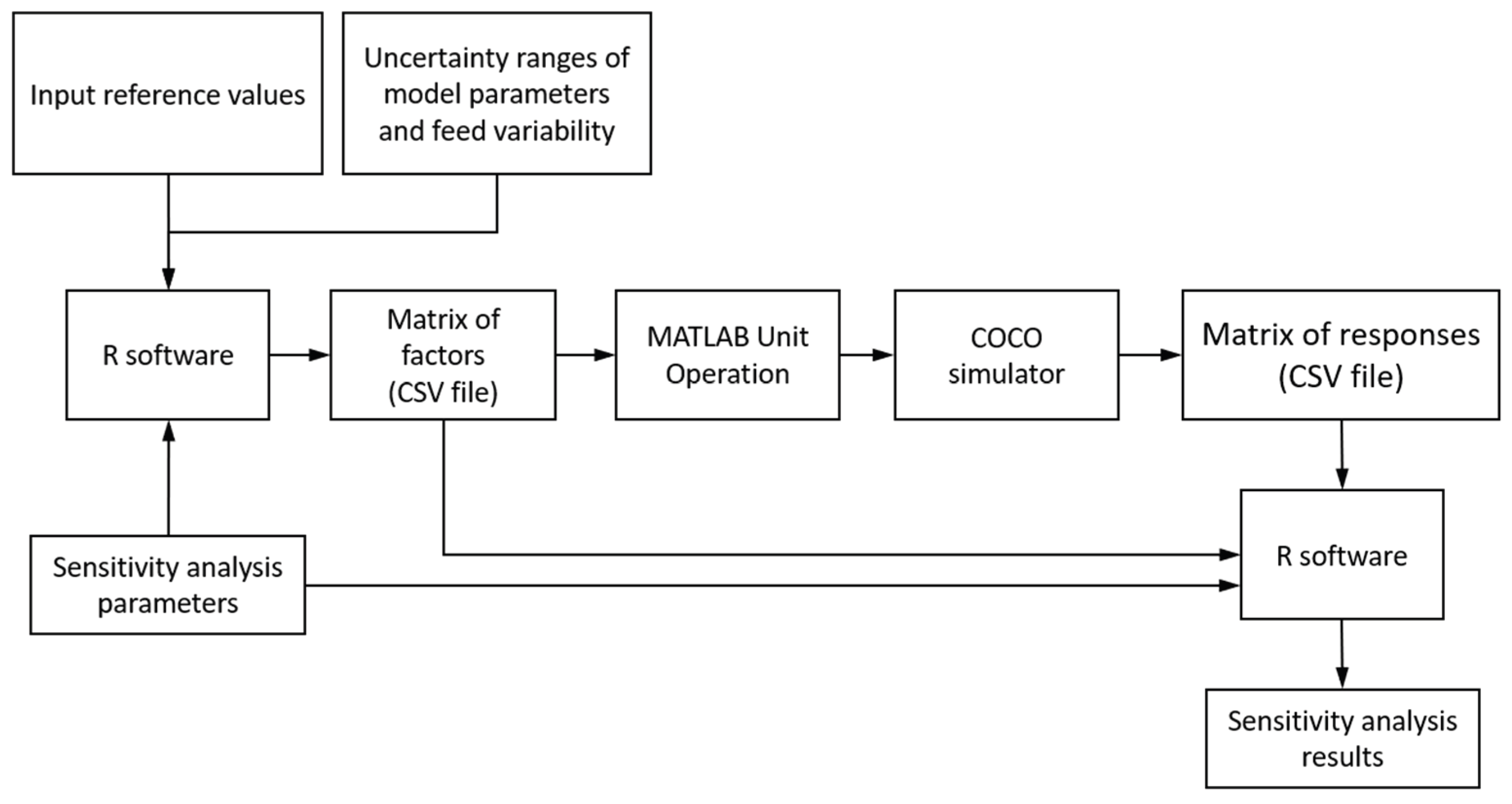
Figure 4.
Morris design with optimized trajectories obtained in R.
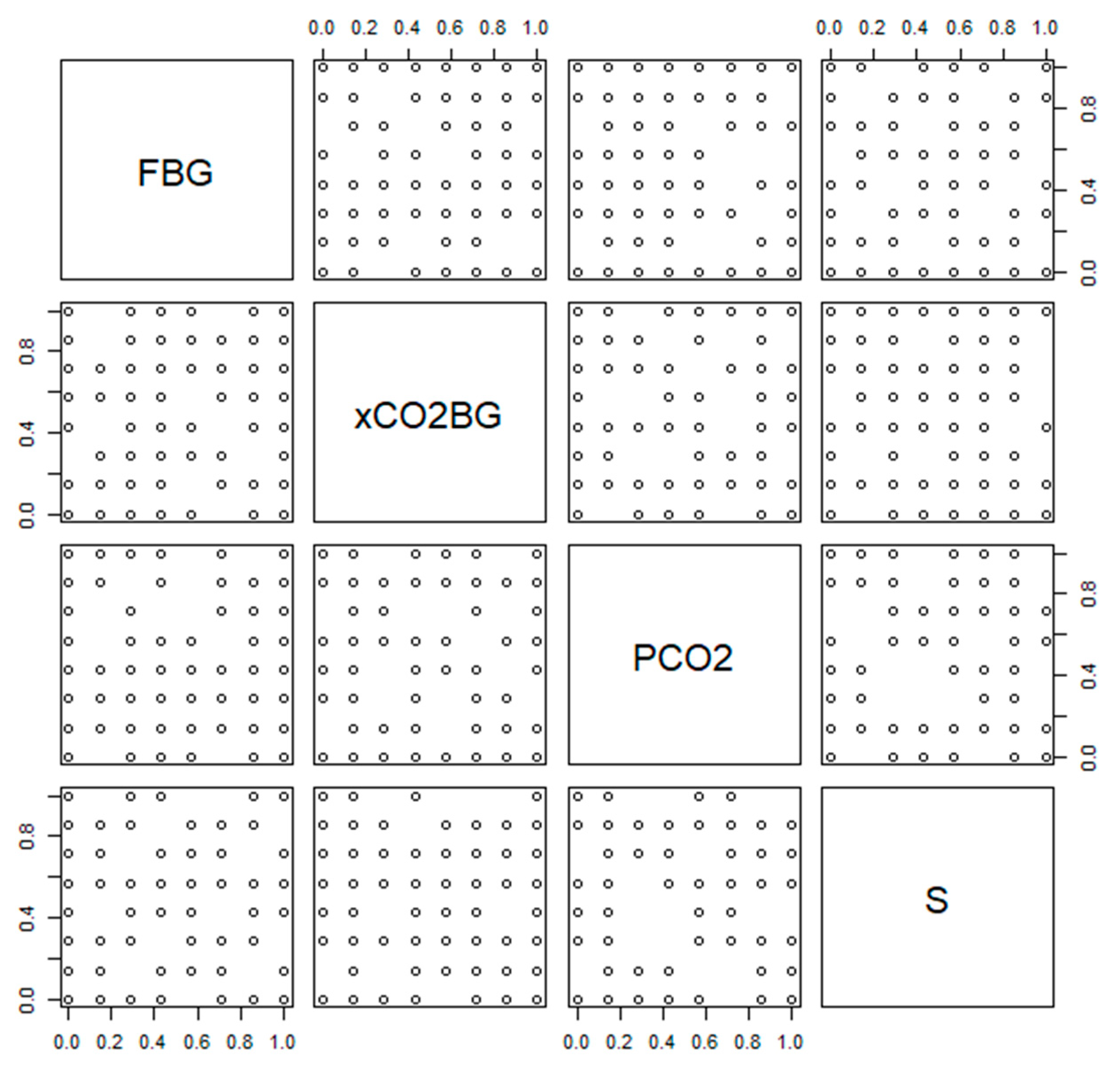
Figure 5.
Morris’ results of the normalized flow of the biomethane product (FBM) for the non-controlled and controlled scenarios at two levels of feed variability (FV).
Figure 5.
Morris’ results of the normalized flow of the biomethane product (FBM) for the non-controlled and controlled scenarios at two levels of feed variability (FV).
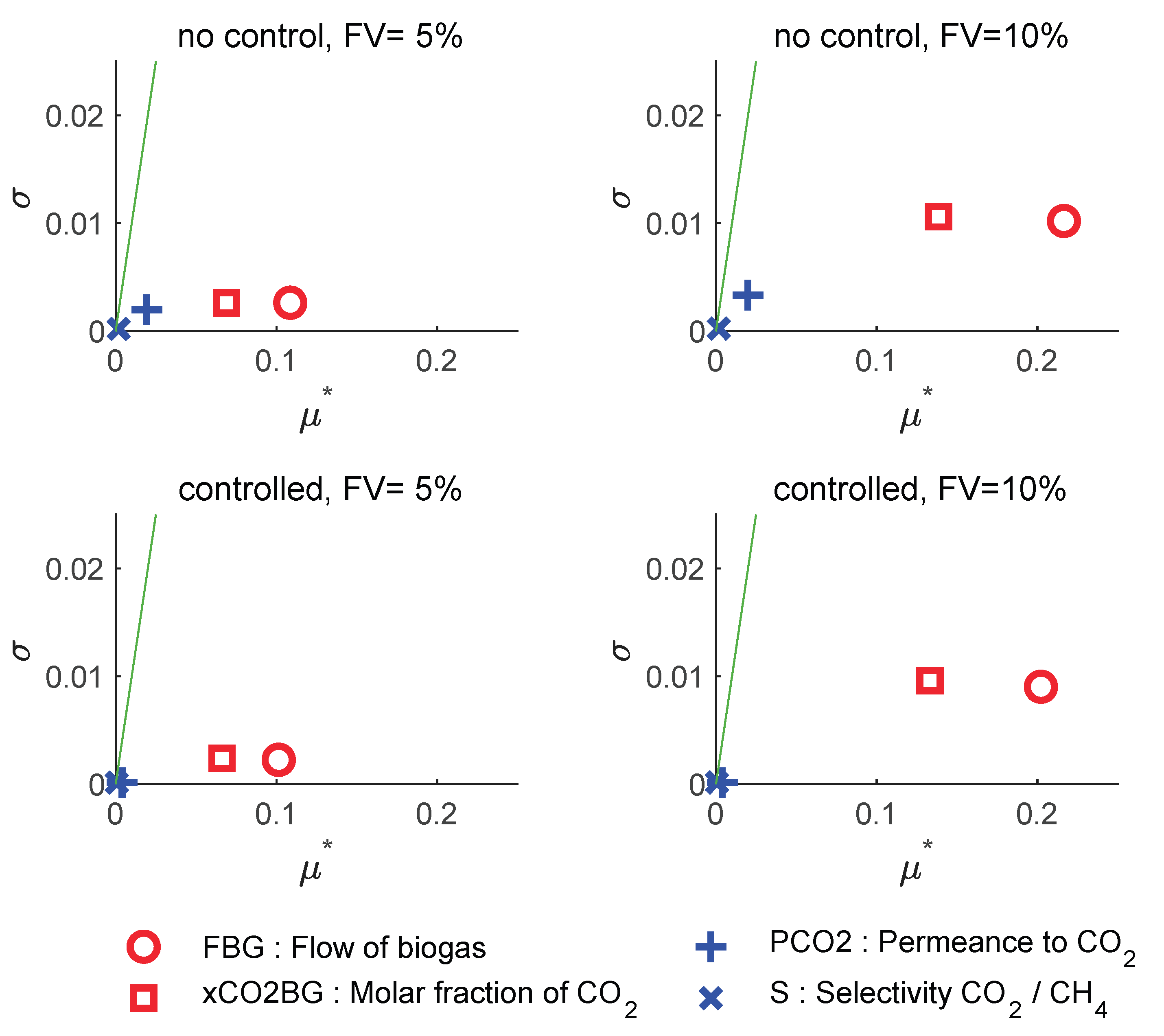
Figure 6.
Morris’ results of the normalized flow of the off-gas stream (FOG) for the non-controlled and controlled scenarios at two levels of feed variability (FV).
Figure 6.
Morris’ results of the normalized flow of the off-gas stream (FOG) for the non-controlled and controlled scenarios at two levels of feed variability (FV).
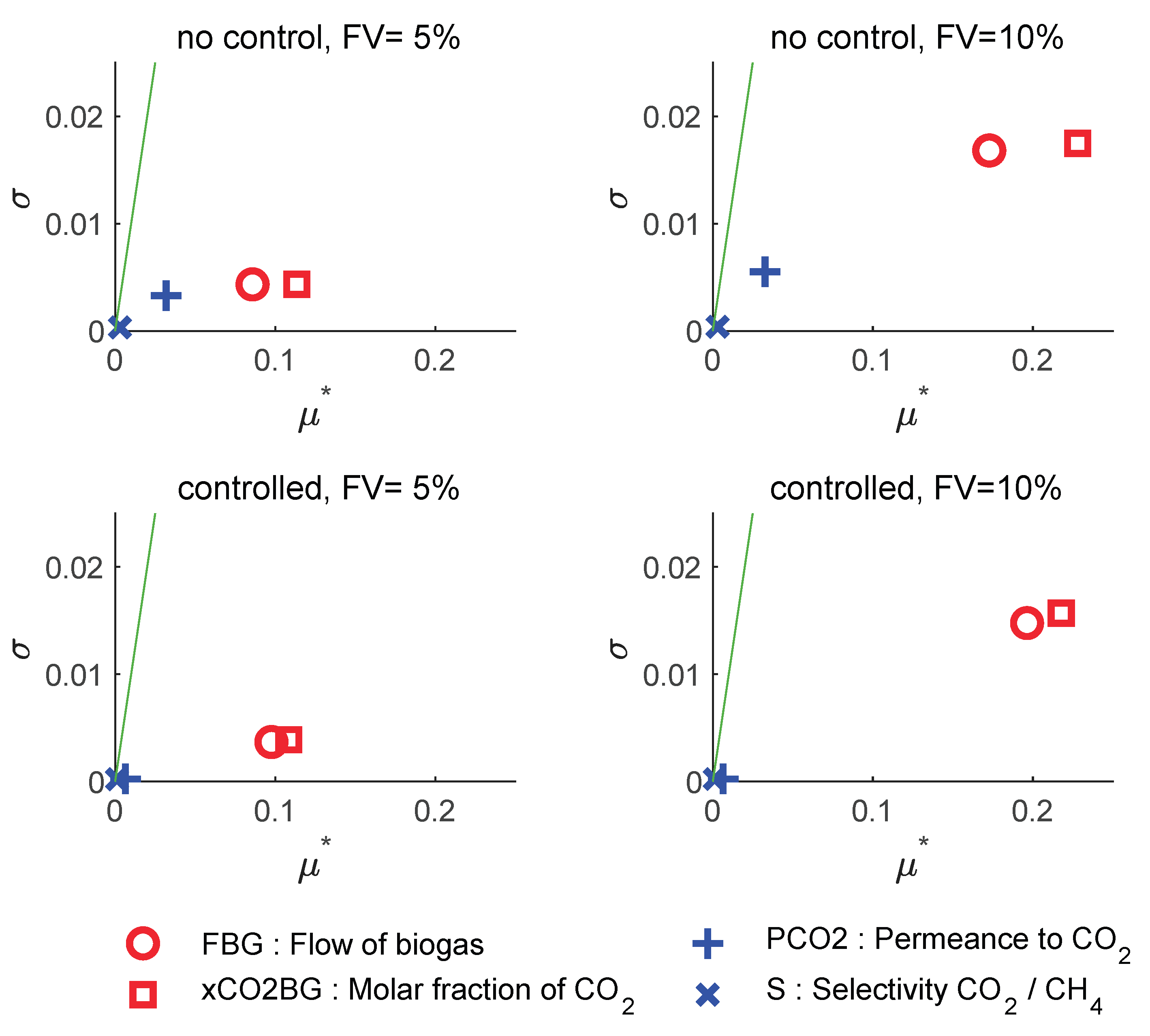
Figure 7.
Morris’ results of CH4 composition of the biomethane product (xCH4BM) for the non-controlled scenario at two feed variability (FV) levels.
Figure 7.
Morris’ results of CH4 composition of the biomethane product (xCH4BM) for the non-controlled scenario at two feed variability (FV) levels.
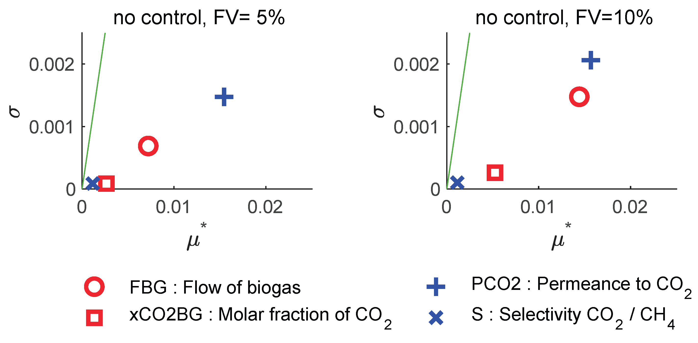
Figure 8.
Morris’ results of the CO2 composition of the off-gas (xCO2OG) for the non-controlled and controlled scenarios at two levels of feed variability (FV).
Figure 8.
Morris’ results of the CO2 composition of the off-gas (xCO2OG) for the non-controlled and controlled scenarios at two levels of feed variability (FV).
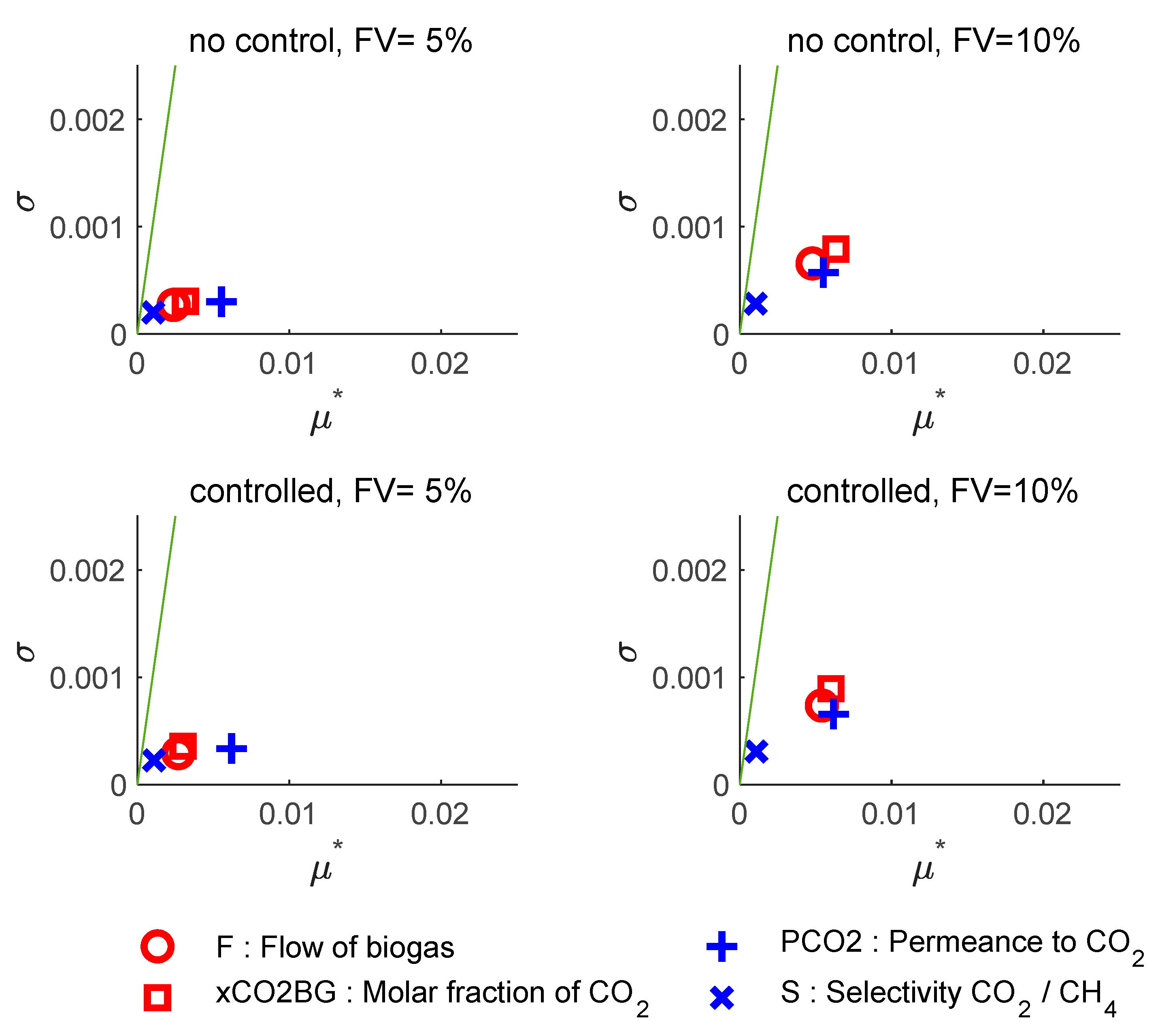
Figure 9.
Morris’ results of the energy demand of the compressor (EDC) for the non-controlled and controlled scenarios at two levels of feed variability (FV).
Figure 9.
Morris’ results of the energy demand of the compressor (EDC) for the non-controlled and controlled scenarios at two levels of feed variability (FV).
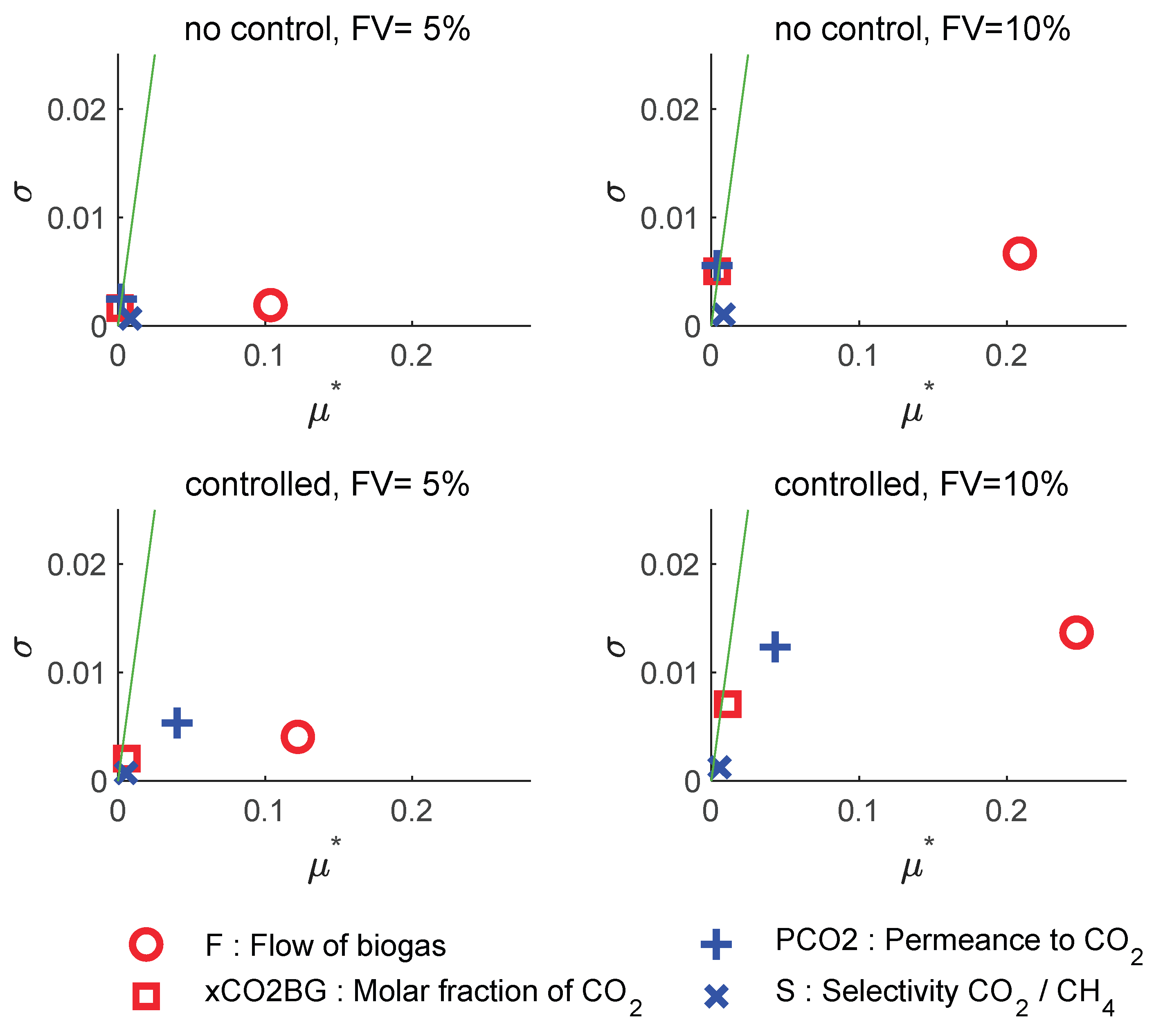
Figure 10.
Morris’ analysis results of the ratio of the energy demand of the compressor to biogas flow (EDC/FBG) for the non-controlled and controlled scenarios at two feed variability (FV) levels.
Figure 10.
Morris’ analysis results of the ratio of the energy demand of the compressor to biogas flow (EDC/FBG) for the non-controlled and controlled scenarios at two feed variability (FV) levels.
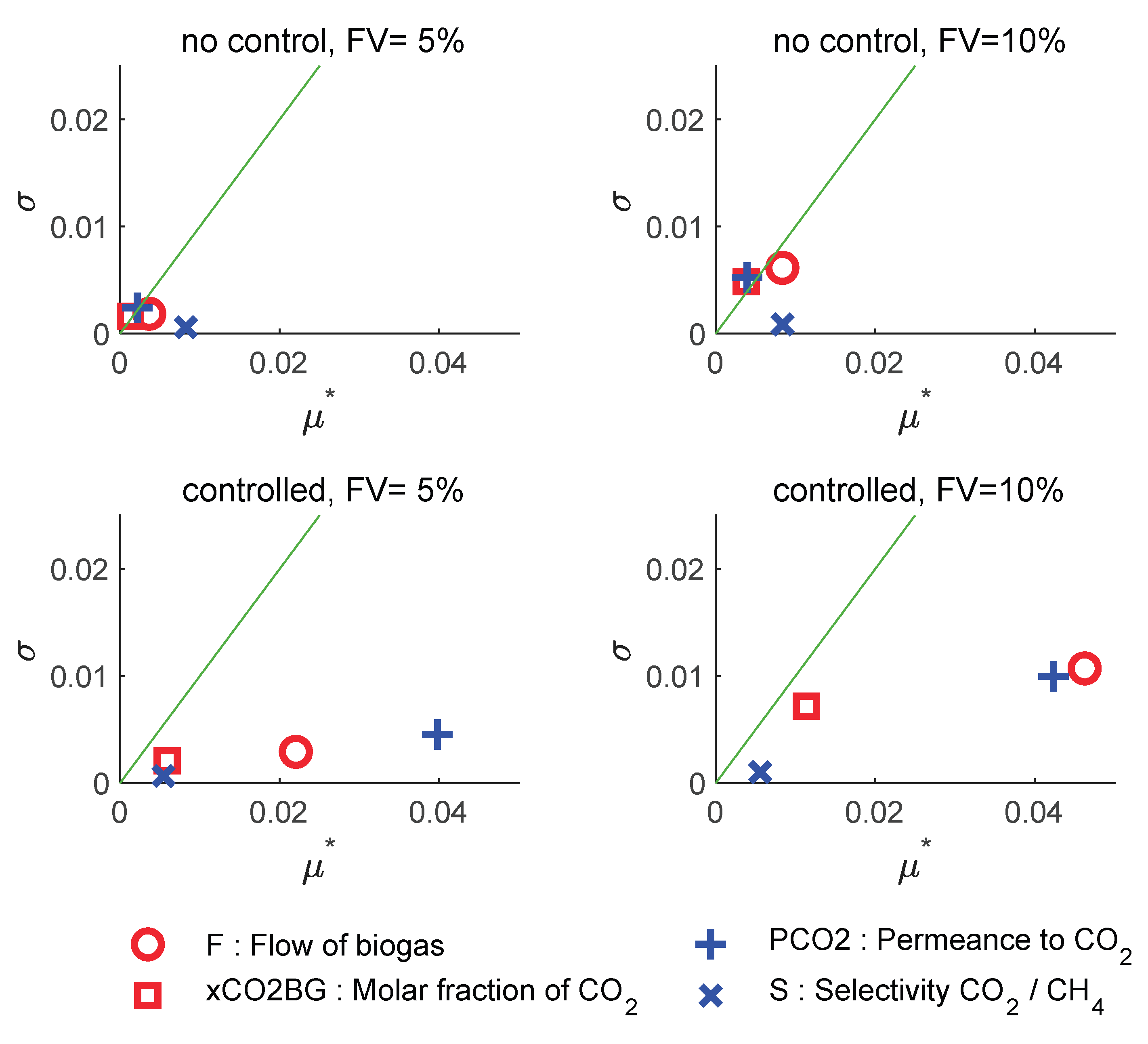

Table 1.
References values for case study [14].
Table 1.
References values for case study [14].
| Parameter Description | Nominal Value |
|---|---|
| Feed flow | 6692 mol/h |
| Mole fraction of CH4 in the feed | 0.6 |
| Mole fraction of CO2 in the feed | 0.4 |
| CO2/CH4 selectivity | 60 |
| CO2 permeance | 60 GPU |
| Retentate pressure (stage 2) | 16.0 bar |
| Permeate pressure (stage 1) | 3.3 bar |
| Permeate pressure (stages 2 and 3) | 1.0 bar |
| Area stage 1 | 167 m2 |
| Area stage 2 | 164 m2 |
| Area stage 3 | 254 m2 |
Table 2.
Uncertainty factors considered in this study.
| Parameter | Description | Reference Value | Variation |
|---|---|---|---|
| FBG | Flow of biogas | 6692 mol/h | ±5%, ±10% of reference |
| xCO2BG | CO2 molar fraction of biogas | 40% | ±5%, ±10% |
| PCO2 | CO2 membrane permeance | 60 GPU | ±10% |
| S | CO2/CO4 selectivity | Eq. 6 applied to 60 | ±5% |
Table 3.
Response variables studied.
| Response variable 1 | Definition |
|---|---|
| FBM | Molar flow of the upgraded biomethane (retentate of unit MB2) |
| xCH4BM | CH4 fraction of the upgraded biomethane |
| FOG | Molar flow of the off-gas stream (permeate of unit MB3) |
| xCO2OG | CO2 fraction of the off-gas stream |
| EDC | Energy demand of compressor CP |
| HDX | Heat duty of heat exchanger HX |
Table 4.
Response values for the two operating scenarios and the reference values of the case study.
Table 4.
Response values for the two operating scenarios and the reference values of the case study.
| Response | Non-Controlled Scenario | Controlled Scenario |
|---|---|---|
| FBM | 4163 mol/h | 4154 mol/h |
| FOG | 2529 mol/h | 2538 mol/h |
| xCH4BM | 0.9579 | 0.9600 |
| xCO2OG | 0.9890 | 0.9891 |
| EDC | 29.95 kW | 30.12 kW |
| HDX | -29.78 kW | -29.97 kW |
| EDC/FBG | 16.11 kJ/mol | 16.21 kJ/mol |
| HDX/FBG | -16.02 kJ/mol | -16.12 kJ/mol |
Table 5.
Properties of the probability distribution of the response variables for the controlled (C) and non-controlled (NC) scenarios at two levels of feed variability (FV). LTL and UTL are respectively the lower and upper tolerance limits of the interval that covers 95% probability content.
Table 5.
Properties of the probability distribution of the response variables for the controlled (C) and non-controlled (NC) scenarios at two levels of feed variability (FV). LTL and UTL are respectively the lower and upper tolerance limits of the interval that covers 95% probability content.
| Response | Units | Sc. | FV | Mean | LTL | UTL | RLG 1 | RUG 2 | CV 3 |
|---|---|---|---|---|---|---|---|---|---|
| FBM | mol/h | NC | ±5% | 4161 | 3829 | 4502 | 7.98% | 8.19% | 3.75% |
| NC | ±10% | 4159 | 3510 | 4812 | 15.61% | 15.70% | 7.45% | ||
| C | ±5% | 4151 | 3837 | 4438 | 7.57% | 6.93% | 3.50% | ||
| C | ±10% | 4148 | 3532 | 4731 | 14.86% | 14.06% | 7.01% | ||
| FOG | mol/h | NC | ±5% | 2525 | 2305 | 2753 | 8.72% | 9.03% | 4.20% |
| NC | ±10% | 2521 | 2116 | 2974 | 16.05% | 17.98% | 8.25% | ||
| C | ±5% | 2535 | 2325 | 2761 | 8.30% | 8.91% | 4.21% | ||
| C | ±10% | 2532 | 2119 | 2991 | 16.28% | 18.14% | 8.41% | ||
| xCH4BM | ‒ | NC | ±5% | 0.9577 | 0.9465 | 0.9657 | 1.17% | 0.84% | 0.45% |
| NC | ±10% | 0.9577 | 0.9426 | 0.9683 | 1.58% | 1.11% | 0.59% | ||
| xCO2OG | ‒ | NC | ±5% | 0.9889 | 0.9848 | 0.9930 | 0.41% | 0.41% | 0.19% |
| NC | ±10% | 0.9887 | 0.9823 | 0.9944 | 0.64% | 0.58% | 0.27% | ||
| C | ±5% | 0.9890 | 0.9846 | 0.9934 | 0.45% | 0.44% | 0.20% | ||
| C | ±10% | 0.9888 | 0.9821 | 0.9948 | 0.67% | 0.60% | 0.29% | ||
| EDC | kW | NC | ±5% | 29.94 | 28.39 | 31.47 | 5.19% | 5.12% | 3.04% |
| NC | ±10% | 29.92 | 26.91 | 32.97 | 10.09% | 10.16% | 6.08% | ||
| C | ±5% | 30.12 | 28.15 | 32.45 | 6.54% | 7.72% | 3.70% | ||
| C | ±10% | 30.11 | 26.63 | 34.27 | 11.57% | 13.80% | 7.22% | ||
| HDX | kW | NC | ±5% | 29.77 | 28.22 | 31.30 | 5.21% | 5.14% | 3.05% |
| NC | ±10% | 29.76 | 26.74 | 32.80 | 10.13% | 10.24% | 6.10% | ||
| C | ±5% | 29.97 | 27.95 | 32.35 | 6.72% | 7.94% | 3.77% | ||
| C | ±10% | 29.96 | 26.42 | 34.18 | 11.82% | 14.09% | 7.33% | ||
| EDC/FBG | kJ/mol | NC | ±5% | 16.12 | 16.03 | 16.21 | 0.56% | 0.53% | 0.27% |
| NC | ±10% | 16.13 | 16.00 | 16.26 | 0.78% | 0.85% | 0.35% | ||
| C | ±5% | 16.22 | 15.84 | 16.69 | 2.33% | 2.89% | 1.23% | ||
| C | ±10% | 16.22 | 15.65 | 16.88 | 3.49% | 4.06% | 1.70% | ||
| HDX/FBG | kJ/mol | NC | ±5% | 16.03 | 15.94 | 16.12 | 0.55% | 0.57% | 0.28% |
| NC | ±10% | 16.04 | 15.91 | 16.19 | 0.76% | 0.96% | 0.37% | ||
| C | ±5% | 16.13 | 15.73 | 16.63 | 2.49% | 3.10% | 1.32% | ||
| C | ±10% | 16.13 | 15.54 | 16.83 | 3.70% | 4.33% | 1.82% |
1 Relative lower-bound gap = (Mean − LTL)/Mean. 2 Relative upper-bound gap = (UTL − Mean)/Mean. 3 Coefficient of variation = Standard deviation / Mean
Disclaimer/Publisher’s Note: The statements, opinions and data contained in all publications are solely those of the individual author(s) and contributor(s) and not of MDPI and/or the editor(s). MDPI and/or the editor(s) disclaim responsibility for any injury to people or property resulting from any ideas, methods, instructions or products referred to in the content. |
© 2025 by the authors. Licensee MDPI, Basel, Switzerland. This article is an open access article distributed under the terms and conditions of the Creative Commons Attribution (CC BY) license (http://creativecommons.org/licenses/by/4.0/).
Copyright: This open access article is published under a Creative Commons CC BY 4.0 license, which permit the free download, distribution, and reuse, provided that the author and preprint are cited in any reuse.


