
Submitted:
25 July 2025
Posted:
29 July 2025
You are already at the latest version
Abstract
This paper proposes a novel pixel-level non-local similarity (PNS)-based reconstruction method for millimeter-wave interferometric synthetic aperture radiometer (InSAR) imaging. Unlike traditional compressed sensing (CS) methods, which rely on predefined sparse transforms and often introduce artifacts, our approach leverages structural redundancies in InSAR images through an enhanced sparse representation model with dynamically filtered coefficients. This design simultaneously preserves fine details and suppresses noise interference. Furthermore, an iterative refinement mechanism incorporates raw sampled data fidelity constraints, enhancing reconstruction accuracy. Simulation and physical experiments demonstrate that the proposed InSAR-PNS method significantly outperforms conventional techniques: it achieves a 1.93 dB average PSNR improvement over CS-based reconstruction while operating at reduced sampling ratios compared to Nyquist-rate FFT methods. The framework provides a practical and efficient solution for high-fidelity millimeter-wave InSAR imaging under sub-Nyquist sampling conditions.
Keywords:
millimeter-wave interferometric synthetic aperture radiometer
; sparse reconstruction
; compressed sensing
; pixel-level non-local similarity
; image reconstruction
1. Introduction
The interferometric synthetic aperture radiometer (InSAR) synthesizes an equivalent large aperture through an array of small-aperture antenna elements, overcoming the spatial resolution limitations inherent in traditional single large-aperture antenna designs and achieving high-resolution real-time imaging [1,2,3]. The ability of millimeter waves to penetrate natural obscurants, such as fog and clouds, enables millimeter-wave InSAR systems to operate in near-all-weather and day-night conditions [4,5]. Additionally, the system’s inherent low observability, stemming from its passive detection principle, coupled with high sensitivity to metallic objects, makes it critical for modern detection systems. As a passive imaging technique, millimeter-wave InSAR finds broad applications in remote sensing, environmental monitoring, and public safety [6,7,8,9].
The core principle of InSAR imaging involves acquiring samples of the visibility function (i.e., complex cross-correlations between antenna pairs) within the spatial-frequency domain, which constitute sampled spatial spectra. To form the final image, the brightness temperature (BT) distribution must be reconstructed by inversely transforming these sampled spatial spectra. This reconstruction achieves high angular resolution determined by the longest baseline, surpassing the diffraction limit of single-aperture systems and is critical to the overall imaging capability [10,11]. Consequently, BT image reconstruction constitutes a crucial step in the InSAR imaging process. Under ideal conditions, the visibility function corresponds to the spatial Fourier transform of the BT distribution. Due to this relationship, the Fast Fourier Transform (FFT) is established as the fundamental reconstruction method for millimeter-wave InSAR imaging [12].
However, practical system implementations face dual technical challenges: on the one hand, the limited number of antennas results in insufficient sampling in the spatial-frequency domain, failing to meet the Nyquist sampling criterion; on the other hand, phase errors and system noise can significantly amplify reconstruction artifacts [13,14]. These two key limitations severely constrain the performance of traditional reconstruction methods (e.g., FFT) under non-ideal conditions. To mitigate these issues, various strategies have been proposed in the literature. For instance, Anterrieu et al. [15] described an algorithm for performing discrete Fourier transform calculations on hexagonal grids and proposed an interpolation formula to resample data from such grids without introducing aliasing artifacts. In a separate approach, Zhou et al. [16] introduced an iterative method for BT image reconstruction from non-uniformly sampled visibility function data. This method combined the conjugate gradient algorithm with a min-max non-uniform FFT approach to enhance image quality. While these engineering solutions offer some mitigation of the aforementioned shortcomings, traditional reconstruction methods (including enhanced FFT and its variants) still suffer from significant image degradation under high-noise scenarios or conditions of severe undersampling.
Compressed sensing (CS) emerged to address undersampling by exploiting scene sparsity. Based on the inherent sparsity of InSAR images, CS technology has been successfully applied to InSAR imaging in recent years [6,17,18,19]. It enables effective recovery of BT images from insufficient visibility samples, reducing both receiver count and data requirements while maintaining high resolution compared to FFT [17,18]. However, conventional CS algorithms degrade performance by converting 2D images into 1D vectors for sparse recovery, neglecting the inherent high-dimensional characteristics and structural priors of InSAR data.
To better exploit these high-dimensional priors, non-local self-similarity (NSS) techniques have been introduced. NSS improves upon CS by aggregating similar image patches, leveraging image correlations to achieve lower reconstruction errors and superior visual quality under undersampling [20]. Nevertheless, NSS operates at the patch level, inherently limiting its ability to preserve fine details due to coarse granularity. Recognizing pixels as fundamental image constituents, Hou et al. developed a pixel-level NSS method for magnetic resonance imaging (MRI), employing row-matching similarity modeling to enhance reconstruction fidelity [21]. Notably, while pixel-level NSS has demonstrated cross-domain applicability in InSAR mixed noise suppression [22], its potential for direct InSAR image reconstruction from undersampled data remains unexplored. Building on this gap, we pioneer the integration of pixel-level non-local similarity (PNS) into a dedicated millimeter-wave InSAR reconstruction framework, establishing the novel InSAR-PNS method. The main contributions are summarized as follows:
- 1)
- Incorporation of PNS into millimeter-wave InSAR reconstruction framework, establishing a joint high-dimensional sparse representation model. This approach enhances structural feature extraction through pixel-level similarity mining, addressing detail-preservation limitations inherent in patch-based methods.
- 2)
- Development of an adaptive thresholding strategy for sparse coefficients, which dynamically adjusts parameters based on noise distribution during reconstruction stages. This design enhances robustness against complex noise interference while balancing detail preservation and noise suppression.
- 3)
- Implementation of an iteratively guided reconstruction algorithm that integrates high-dimensional feature learning from initial BT images with raw sampled data fidelity constraints, overcoming error accumulation limitations in conventional approaches.
- 4)
- Validation through simulations and physical experiments, confirming the method’s efficacy and applicability to complex environments in millimeter-wave InSAR imaging.
The rest of this article is organized as follows. Section 2 introduces the basic theoretical principles of millimeter-wave InSAR imaging. Section 3 presents the details of the proposed InSAR-PNS reconstruction method. The simulation and physical experiments are compared and discussed in Section 4. In addition, Section 5 provides the conclusions.
2. Theoretical Principles of Millimeter-Wave InSAR Imaging
Millimeter-wave InSAR imaging technology is based on the well-known Van Cittert-Zernike theorem, and its core component is a binary interferometer [23,24]. The InSAR imaging system utilizes a spatially separated antenna array to form a series of antenna pairs and measures millimeter-wave radiation within the target space and performs complex correlation operations on the collected signals to obtain the visibility function. Subsequently, high-resolution millimeter-wave BT distribution images are reconstructed from the visibility function using reconstruction algorithms such as the FFT method or G-matrix method [25]. The millimeter-wave InSAR imaging processing flow can be shown as Figure 1.
Assume that the radiation source S in the radiation scenario shown in Figure 1 is discretized into M point-source targets, denoted as . Let the distances between the radiation source and antennas and be and , respectively. According to [26,27], the visibility function of the antenna pair ( - ) can be expressed as
where is the BT distribution. is the normalized antenna pattern. is the fringe-washing function taking into account the spatial decorrelation effect of the receiver frequency response, which is approximately equal to 1 for the narrow bandwidth receiver. is the operating wavelength.
Defining the spatial-frequency coordinates and replacing the rectangular coordinates with polar coordinates , Equation (1) can be rewritten as
where .
According to Equation (2), when the requirement on imaging accuracy is not stringent, the most basic BT image reconstruction can be directly achieved by taking an inverse Fourier transform on . Considering the observation errors and InSAR receiving noise, the basic signal model for InSAR imaging can be expressed as
where represents the observation errors and receiving noise.
The reconstruction method that directly performs an inverse Fourier transform on often requires highly rigorous calibration. Otherwise, its performance will degrade due to the presence of observation errors and receiving noise . In order to minimize the interference of with InSAR imaging, an alternative reconstruction method is to use a generalized shock function operator, i.e., the G-matrix model instead of the Fourier transform relationship in Equation (3). The visibility function and BT are represented as vectors while taking into account the errors and noise [28]. Then the approximate discrete linear system of the InSAR image reconstruction model can be rewritten as
where denotes the BT image to be recovered. is the generalized shock function operator. is the actual undersampled visibility function data. is the error and receiver noise.
3. InSAR-PNS Reconstruction Method
This section outlines the theoretical foundations of PNS, introduces the proposed InSAR-PNS reconstruction framework, and specifies the implementation methodology.
3.1. Principle of PNS
Millimeter-wave BT images exhibit inherent low-rank characteristics [29]. From the perspective of prior knowledge, pixels within the image demonstrate strong spatial correlations. A single pixel existing independently lacks practical significance; instead, adjacent pixels collectively constitute textural or structural features. Such structures are extensively distributed across various regions of the image. For instance, regions exhibiting periodic repetition or texture characteristics contain substantial redundant structural information.
The NSS prior plays a pivotal role in fields such as texture synthesis [30,31], image denoising [32,33,34], super-resolution [35,36], and image reconstruction [21]. In denoising applications, the non-local means (NLM) algorithm pioneered NSS utilization, estimating true pixel values through weighted averaging of similar patches. This approach effectively preserves edges and textures while suppressing noise. Patch-level NSS was further advanced in the block-matching and 3D filtering (BM3D) algorithm [33] and subsequent studies [34]. While classical NLM and BM3D exploit patch-level self-similarity, they often disregard intra-patch pixel variations. Given that pixels constitute the fundamental units of images and exhibit intrinsic correlations within patches. Therefore, based on the utilization of the similarity prior at the patch-level, we can further locate and match similar pixels to more comprehensively utilize the similarity prior information, thus achieving pixel-level image processing.
The workflow for identifying non-local similar pixels is as follows: First, extract non-local similar patches and vectorize each patch into column vectors. Then, combine all the column vectors to construct a similar-patch matrix. For each row in the matrix, use the patch-level NSS prior to establish inherent correlations. Subsequently, compute Euclidean distances between matrix rows to locate non-local similar pixels. Figure 2 provides a schematic overview.
For an input image , the procedure for identifying non-locally similar pixels comprises four stages:
1) Non-local patch extraction
Decompose into L overlapping patches of size ()
where , and represents the patch extraction operator.
2) Patch matching
For a reference patch (yellow-framed in Figure 2), identify similar patches (purple-framed) within a search window (blue-framed) by minimizing the Euclidean distance:
Select the most similar patches. Vectorize each patch ( ) and concatenate them with the reference patch to form a patch-similarity matrix:
3) Row matching
For each row vector in the patch-similarity matrix (representing geometrically corresponding pixels across patches), compute Euclidean distances to other rows:
Select g rows with minimal distances to form a pixel-similarity submatrix:
where , .
4) Iteration
Repeat steps 2-3 for all reference patches.
3.2. InSAR-PNS Reconstruction Model
In InSAR imaging, although the FFT algorithm can achieve BT image reconstruction, it requires full visibility function sampling, necessitating a full populated antenna array. This constraint severely limits the practical application of millimeter-wave InSAR imaging. CS-based imaging algorithm can reconstruct images from undersampled visibility function, which can be measured with a smaller number of antennas. The CS reconstruction model is formulated as:
where represents the sparse vector of the BT image , which needs to be recovered from the sparse basis matrix . Additionally, is the observation matrix, representing the sampling operation on the BT image under various sampling modes. Moreover, denotes the actual undersampled data of the visibility function.
Traditional CS-based InSAR reconstruction techniques utilize the sparsity of millimeter-wave InSAR images. These methods employ predefined sparse transforms (e.g., wavelet, discrete cosine transform) to represent 2D InSAR images as vectors and complete the reconstruction in the 1D data space. The final outputs are reshaped to match original image dimensions. This means that CS-based reconstruction methods cannot utilize high-dimensional signal features and prior knowledge, often fail to provide sufficient sparse representations for the images to be reconstructed. From a Bayesian perspective, sparsity regularization is crucial importance in CS-InSAR imaging. To comprehensively capture high-dimensional priors in BT images, we design a PNS-based sparsifying operator and formulate the InSAR-PNS reconstruction model:
where is the regularization parameter, which is used to balance sparsity ( - norm) and data fidelity ( - norm).
The PNS-derived operator enforces structural sparsity constraints through pixel-level correlations. This model allows us to establish a general formula to balance the sparsity of these patches based on data consistency and provides the feasibility of integrating prior information learned from undersampled data, thus optimizing the sparse representation of the images to be reconstructed.
3.3. InSAR-PNS Reconstruction Algorithm
As Figure 3 shows, the PNS-based InSAR image reconstruction framework comprises two parts: pixel-level non-local sparsification optimization (PNSO) and iterative refinement (IR). Given undersampled measurement data , we first apply zero-padding to generate full-sized spatial-frequency domain data . Subsequently, by performing an inverse FFT on , we obtain a preliminarily reconstructed BT image .
However, this initial reconstruction typically suffers from aliasing artifacts and noise. Therefore, to improve reconstruction quality and exploit pixel-level self-similarity in the image, we introduce PNS before transformation. This allows construction of an adaptive sparsifying transform operator that facilitates pixel-level non-local coefficient updates, generating optimized images . This procedure can not only recover undersampled signals, suppress artifacts, but also maintain image sparsity. Next, FFT converts to spatial-frequency domain data . Crucially, during each iteration, we update the k-th reconstruction’s frequency components in the originally zero-padded positions of , ensuring data fidelity at sampled locations. The visibility function update during iteration k is formulated as:
PNS sparse optimization is primarily based on lifting Haar wavelet transform (LHWT) and performs adaptive double hard-thresholding on sparse coefficients of the pixel similarity matrix. For the initial InSAR BT image requiring optimization, this process follows the pixel similarity matrix search procedure detailed in Section 3.1. Non-local patches are first extracted. Subsequently, within a local search window, the most similar patches are identified to construct a patch similarity matrix . For each row in , g similar rows are selected to form a pixel similarity matrix , Then, the LHWT is applied to to generate sparse coefficients:
where represents the LHWT. Apply the first hard-thresholding on :
where , denote the row and column indices of ; represents the filtering coefficient; and is the threshold parameter. During iterations, decays logarithmically:
where denotes the natural logarithm, represents the noise variance estimation of the initial image , and k is the iteration index, thereby progressively reducing hard-thresholding intensity. Early iterations primarily suppress dominant artifacts, while later stages focus on eliminating residual noise and preserving textural details.
According to wavelet theory [37], the coefficients in the last two rows (excluding column 1) of the coefficient matrix correspond to high-frequency components dominated by artifacts and noise. Consequently, we apply a secondary hard-thresholding operation:
Subsequently, apply the inverse LHWT to :
where denotes the inverse LHWT operator.
4. Experimental Results and Discussion
This section validates the efficacy of the proposed InSAR-PNS reconstruction method through simulated and physical imaging systems. Comparative analysis includes the traditional modified fast Fourier transform (MFFT) and CS-based reconstruction. Experiments were conducted in MATLAB 2020a on a workstation with an Intel® Core™ i7-10750H CPU and 16 GB RAM.
4.1. Simulation Platform Experiments
An InSAR imaging simulation model was implemented to emulate the millimeter-wave propagation and data acquisition chain. As depicted in Figure 1, this model comprehensively simulates the entire imaging process, including target radiation, antenna array visibility sampling, cross-correlation computation between antenna pairs, visibility function generation, and BT image reconstruction.
The simulation process started with millimeter-wave radiation source modeling, where each discrete point source was derived from two ideal scenes, as shown in Figure 4(a) and Figure 5(a). The image dimension is 100×100 pixels, and the gray value of each pixel represents the intensity of the radiation emitted from a discrete point source. Subsequently, in-phase and quadrature(IQ) signals were acquired through coherent integration across the simulated scene. According to Equation (1), complex cross-correlation was applied to compute the visibility function V. Following phase compensation of the visibility data, the calibrated visibility function was generated. The BT image was ultimately reconstructed from using different inversion algorithms.
The system operates at 100 GHz () and employs a T-shaped antenna array configuration comprising 150 elements. The inter-element spacing was set to 12 mm (), yielding a equivalent synthetic aperture. The specific simulation parameters are shown in Table 3. The MFFT method reconstructs BT images using the full set of visibility function samples, as demonstrated in Figure 4(b) and Figure 5(b). In contrast, the CS and InSAR-PNS methods employ reduced sampling rates of 90% to 40%. Specifically, Figure 4(c) and Figure 5(c) present reconstruction results for both methods at 80% sampling rate, while Figure 4(d) and Figure 5(d) correspond to results at 50% sampling rate.
Comparative analysis of the reconstruction results in Figure 4 and Figure 5 demonstrates that the proposed InSAR-PNS method (Figure 4(d) and Figure 5(d)) outperforms both the MFFT (Figure 4(b) and Figure 5(b)) and CS (Figure 4(c) and Figure 5(c)) methods in terms of visual clarity, contour preservation, and target detail representation. The MFFT method exhibits performance degradation due to constraints from discrete and finite antenna array sampling, while the CS method, limited by fixed sparse basis, fails to learn high-dimensional features of BT images. Notably under 50% sampling, CS method shows a significant quality deterioration (Figure 5(c)), whereas the InSAR-PNS method maintains high-fidelity BT images with preserved fine details (Figure 5(d)) through its iterative adaptive learning mechanism.
During practical imaging, noise interference and measurement errors are inevitable, primarily caused by hardware inconsistencies, antenna position deviations, and system noise. To simulate complex imaging environments, we employ zero-mean Gaussian white noise with varying variances to characterize interference factors. To evaluate the robustness of the InSAR-PNS method, Gaussian white noise with varying intensities was added to the visibility function samples corresponding to the BT image shown in Figure 5(a), simulating actual noise-corrupted imaging processes. Figure 6(a)-(c) respectively display BT images reconstructed under low-intensity interference () using: (a) MFFT with full visibility function samples; (b) CS with 80% visibility samples; (c) InSAR-PNS with 80% visibility samples. Figure 6(d)-(f) respectively show BT images reconstructed under high-intensity interference () using: (d) MFFT with full visibility samples; (e) CS with 80% visibility samples; (f) InSAR-PNS with 80% visibility samples.
Analysis the reconstruction results in Figure 6 demonstrates that the MFFT output experiences severe noise degradation, nearly failing to preserve target contour information (Figure 6(d)) due to its lack of noise suppression capability and susceptibility to the Gibbs phenomenon. Conversely, both CS and InSAR-PNS reconstructions exhibit superior visual performance. Specifically, the InSAR-PNS method retains target contours and provides rich detail while suppressing noise contamination under strong interference conditions ().
In addition, Figure 7 summarizes the peak signal-to-noise ratio (PSNR) values of MFFT, CS, and InSAR-PNS under varying sampling rates and noise levels. The data indicate that as the sampling rate decreases, InSAR-PNS demonstrates superior performance compared to CS. Concurrently, the PSNR values of all three algorithms decline with increasing noise intensity, reflecting a degradation in algorithmic performance. This deterioration is primarily attributed to the increasing dominance of noise components. Although heightened noise intensity poses greater challenges for reconstruction tasks, the proposed method (InSAR-PNS) consistently outperforms the other algorithms in terms of performance.
4.2. Physical Imaging System Experiments
In millimeter-wave InSAR imaging research, discrepancies persist between simulation environments and actual physical systems. Practical systems are frequently subject to non-ideal constraints such as hardware mismatches and environmental noise, leading to deviations in imaging outcomes from simulation predictions. Consequently, experimental validation using physical platforms becomes imperative.
Leveraging the principles of millimeter-wave InSAR imaging, a two-element interferometer enables 2D imaging through baseline scanning when imaging speed is not the primary concern. Owing to its minimalist architecture and cost-effective design, this configuration constitutes a standard testbed for algorithm verification in millimeter-wave InSAR studies. This work utilizes a T-shaped mechanically-scanned millimeter-wave InSAR system equipped with a two-element interferometer to assess the reconstruction performance of the proposed algorithm. Key system parameters are detailed in Table 4.
The physical implementation of the system is presented in Figure 8. Full spatial baseline sampling within the observation airspace is achieved through independent displacement of two array elements along orthogonal horizontal and vertical axes. The correlator receiver integrates two identical 3-mm wavelength radiometers, each consisting of a receiving antenna, front-end module, intermediate-frequency (IF) module, and local oscillator (LO) module.
The antenna unit employs two small-aperture conical horn antennas to capture radiation from the observed scene. The front-end module amplifies received signals and suppresses image band interference through bandpass filtering. Signals are then downconverted to the IF band by mixing with a 16.7 GHz LO reference. Within the IF stage, the analog signals are subjected to quadrature demodulation to generate IQ components, which are forwarded to the digital processing unit. Following Analog-to-Digital Conversion, the digitized I/Q signals undergo cross-correlation to generate visibility function samples. These samples are transferred to a host computer for storage, processing, and rendering the reconstructed images using the BT reconstruction algorithm.
Subsequently, the effectiveness of the proposed InSAR reconstruction algorithm was validated using the scanning imaging system designed in this study. The test configurations are illustrated in Figure 8(c) and (d): Figure 8(c) depicts the imaging scenario for a vehicle at 6 m under clear-weather and weak interference conditions, while Figure 8(d) shows the imaging scenario for a human subject carrying a metallic disc at 3.3 m under cloudy conditions with textile occlusion.
Figure 9 and Figure 10 comparably demonstrate the reconstruction characteristics of different methods: (a) displays the optical reference images of the targets, and (b) to (d) respectively show the reconstruction results of MFFT full sampling, CS, and InSAR-PNS 70% sparse sampling.
Experimental results indicate that, under both strong and weak interference environments, InSAR-PNS can achieve superior reconstruction fidelity compared to both MFFT and CS methods. The method generates smooth-textured images that preserve essential features of BT images, exhibiting well-defined boundaries with suppressed background noise. This demonstrates that the proposed InSAR-PNS method has strong adaptability to complex environments, validating its efficacy and practical utility in physical millimeter-wave InSAR applications.
5. Conclusions
In this study, we propose a novel InSAR reconstruction method based on pixel-level non-local similarity (InSAR-PNS), with its reconstruction performance validated through simulations and practical millimeter-wave InSAR systems. Building upon millimeter-wave InSAR imaging principles, we introduce pixel-level non-local similarity matching mechanism to construct an enhanced sparse representation model. This model leverages high-dimensional prior information from non-local similarity and dynamically optimizes threshold coefficients to effectively preserve image details while suppressing noise interference. Through iterative refinement design, the algorithm simultaneously retains raw sampled data to enhance reconstruction accuracy.
Experimental results demonstrate that, compared to traditional FFT methods requiring full sampling without calibration strategies, InSAR-PNS achieves an average PSNR gain of 5.88 dB across varying noise variances, with advantages amplifying under intensified interference. When benchmarked against CS reconstruction using fixed sparse dictionaries, InSAR-PNS exhibits an average PSNR improvement of 1.93 dB across different sampling rates. Both visual evaluation and quantitative analysis confirm that the proposed InSAR-PNS reconstruction method exhibits superior performance in improving reconstruction quality and noise suppression, providing a robust solution for millimeter-wave InSAR imaging in complex environments.
Author Contributions
Conceptualization, J.Y., Q.L. and Y.L.; methodology, J.Y., Z.C. Q.L. and Y.L.; software, Y.J. and Z.C.; validation, Y.J; formal analysis, J.Y., Z.C. Q.L. and Y.L.; investigation, Y.J; resources, J.Y., Q.L. and Y.L.; data curation, J.Y.; writing—original draft preparation, J.Y.; writing—review and editing,J.Y., Z.C. Q.L. and Y.L.; visualization, J.Y.; supervision, Q.L. and Y.L.; project administration, J.Y., Z.C. Q.L. and Y.L.; funding acquisition, Q.L. All authors have read and agreed to the published version of the manuscript.
Funding
This work was supported in part by the Natural Science Research of Jiangsu Higher Education Institutions of China under Grant 22KJA510001 and in part by the Open Project of the State Key Laboratory of Millimeter Waves under Grant K202406.
Data Availability Statement
No new data were created.
Acknowledgments
The authors acknowledge the Section Managing Editor and anonymous reviewers for their insightful feedback and valuable recommendations.
Conflicts of Interest
The authors declare no conflicts of interest.
References
- Fu, P.; Zhu, D.; Hu, F.; Xu, Y.; Xia, H. A Near-Field Imaging Algorithm Based on Angular Spectrum Theory for Synthetic Aperture Interferometric Radiometer. IEEE Transactions on Microwave Theory and Techniques 2022, 70, 3606–3616. [Google Scholar] [CrossRef]
- Zhu, T.; Yang, X.; Yan, J.; Wu, L.; Jiang, M.; Wei, B. A MAP Approach With Huber-MRF for Synthetic Aperture Interferometric Radiometer. IEEE Geoscience and Remote Sensing Letters 2024, 21, 1–5. [Google Scholar] [CrossRef]
- He, M.; Yin, X.; Li, Y.; Liu, H.; Zhang, H.; Ren, J.; Wang, S.; Zhou, W. An Improved Reconstruction Technique for Resolution Enhancing of Spaceborne 1-D Interferometric Microwave Radiometer. IEEE Transactions on Geoscience and Remote Sensing 2025, 63, 1–13. [Google Scholar] [CrossRef]
- Sun, X.; Salmon, N.A.; Miao, J. Performance Analysis of a Walk-Through Portal Array for Passive Millimeter-Wave 3-D Imaging. IEEE Transactions on Instrumentation and Measurement 2024, 73, 1–15. [Google Scholar] [CrossRef]
- Fang, B.; Zhu, D.; Hu, F.; Xu, Y.; Hao, Y.; Chen, X.; Tao, J.; Min, J.; Zheng, B. Target Detection Based on Regional Feature Difference in Synthetic Aperture Interferometric Radiometer. IIEEE Transactions on Geoscience and Remote Sensing 2025, 63, 1–12. [Google Scholar] [CrossRef]
- Wu, C.; Wei, Z.; Bi, H.; Zhang, B.; Lin, Y.; Hong, W. InSAR imaging based on L1 regularisation joint reconstruction via complex approximated message passing. Electronics Letters. 2018, 54, 237–239. [Google Scholar] [CrossRef]
- Lyu, J.; Bi, D.; Li, X.; Xie, Y.; Xie, X. Super-resolution image reconstruction of compressive 2D near-field millimetre-wave. Electronics Letters. 2020, 56, 978–980. [Google Scholar] [CrossRef]
- Khazâal, A.; Faucheron, R.; Rodríguez-Fernández, N.J.; Anterrieu, E. Deep-Learning-Based Approach in Imaging Radiometry by Aperture Synthesis: Application to Real SMOS Data. IEEE Journal of Selected Topics in Applied Earth Observations and Remote Sensing 2025, 18, 9321–9332. [Google Scholar] [CrossRef]
- Zhao, Y.; Si, W.; Hu, A.; Miao, J. A Novel Antenna Array Design Method Based on Antenna Grouping for Near-Field Passive Millimeter-Wave Imaging. IEEE Antennas and Wireless Propagation Letters 2024, 23, 399–403. [Google Scholar] [CrossRef]
- Xu, Y.; Zhu, D.; Hu, F.; Fang, B.; Gao, T. A Principal Component Analysis Perspective for RFI Mitigation in Synthetic Aperture Interferometric Radiometer. IEEE Transactions on Geoscience and Remote Sensing 2024, 62, 1–12. [Google Scholar] [CrossRef]
- Yang, X.; Lu, C.; Yan, J.; Wu, L.; Liu, F.; Jiang, M. Iterative Regularization Using an Acceleration Technique for Synthetic Aperture Interferometric Radiometer. IEEE Journal of Selected Topics in Applied Earth Observations and Remote Sensing 2023, 16, 4649–4657. [Google Scholar] [CrossRef]
- Ruf, C.S.; Swift, C.T.; Tanner, A.B.; Le Vine, D.M. Interferometric synthetic aperture microwave radiometry for the remote sensing of the Earth. IEEE Transactions on Geoscience and Remote Sensing. 1988, 26, 597–611. [Google Scholar] [CrossRef]
- Zhang, Y.; Li, Y.; Chen, J.; Shahir, S.; Safavi-Naeini, S. Sparse millimeter-wave InSAR imaging approach based on MC. IEEE Geoscience and Remote Sensing Letters. 2018, 15, 714–718. [Google Scholar] [CrossRef]
- Zhang, Y.; Ren, Y.; Miao, W.; Lin, Z.; Gao, H.; Shi, S. Microwave SAIR Imaging Approach Based on Deep Convolutional Neural Network. IEEE Transactions on Geoscience and Remote Sensing 2019, 57, 10376–10389. [Google Scholar] [CrossRef]
- Anterrieu, E.; Waldteufel, P.; Lannes, A. Apodization functions for 2-D hexagonally sampled synthetic aperture imaging radiometers. IEEE Transactions on Geoscience and Remote Sensing. 2002, 40, 2531–2542. [Google Scholar] [CrossRef]
- Zhou, X.; Sun, H.; He, J.; Lu, X. NUFFT-Based Iterative Reconstruction Algorithm for Synthetic Aperture Imaging Radiometers. IEEE Geoscience and Remote Sensing Letters. 2009, 6, 273–276. [Google Scholar] [CrossRef]
- Chen, J.; Li, Y. . The CS-Based imaging algorithm for near-Field synthetic aperture imaging radiometer. IEICE Transactions on Electronics. 2014, 97, 911–914. [Google Scholar] [CrossRef]
- Wang, J.; Gao, Z.; Gu, J.; Li, S.; Zhang, X.; Dong, Z.; et al. A New Passive Imaging Technique Based on Compressed Sensing for Synthetic Aperture Interferometric Radiometer. IEEE Geoscience and Remote Sensing Letters 2020, 17, 1938–1942. [Google Scholar] [CrossRef]
- Xu, Y.; Zhu, D.; Hu, F.; Fang, B.; Fu, P. Target Imaging Using Compressed Sampling in Synthetic Aperture Interferometric Radiometer. IEEE Transactions on Geoscience and Remote Sensing 2023, 61, 1–15. [Google Scholar] [CrossRef]
- Qu, X.; Hou, Y.; Lam, F.; Guo, D.; Zhong, J.; Chen, Z. Magnetic resonance image reconstruction from undersampled measurements using a patch-based nonlocal operator. Medical image analysis. 2014, 18, 843–856. [Google Scholar] [CrossRef]
- Hou, H.; Shao, Y.; Geng, Y.; Hou, Y.; Ding, P.; Wei, B. PNCS: Pixel-level non-local method based compressed sensing undersampled MRI image reconstruction. IEEE Access. 2023, 11, 42389–42402. [Google Scholar] [CrossRef]
- Yang, J.; Li, Y. A Novel Passive Millimeter Wave Image Noise Suppression Method Based on Pixel Non-local Self-similarity. Progress In Electromagnetics Research M. 2023, 120, 55–67. [Google Scholar] [CrossRef]
- Chen, J.; Ruan, Y.; Yu, J.; Zhang, C.; Zheng, Z.; Zhu, S.; Liu, L. Enhancing Synthetic Aperture Interferometric Radiometer Performance Through Imaging Quality-Centric Array Optimization. IEEE Transactions on Geoscience and Remote Sensing 2025, 63, 1–12. [Google Scholar] [CrossRef]
- Chen, J.; Yu, J.; Ruan, Y.; Zhang, C.; Zheng, Z.; Cai, F.; Zhu, S.; Liu, L. Super-Resolution Imaging Method for Synthetic Aperture Interferometric Radiometer Based on Spectral Extrapolation. IEEE Geoscience and Remote Sensing Letters 2025, 22, 1–5. [Google Scholar] [CrossRef]
- Chen, J.; Zhou, J.; Peng, R. Distance Adaptive Imaging Algorithm for Synthetic Aperture Interferometric Radiometer in Near-Field. IEEE Geoscience and Remote Sensing Letters 2023, 20, 1–5. [Google Scholar] [CrossRef]
- Corbella, I.; Duffo, N.; Vall-llossera, M.; Camps, A.; Torres, F. The Visibility Function in Interferometric Aperture Synthesis Radiometry. IEEE Transactions on Geoscience and Remote Sensing 2004, 42, 1677–1682. [Google Scholar] [CrossRef]
- Shi, T.; Jin, R.; Ren, J.; Chen, K.; Huang, Q.; Li, Q. An Improved Method of Multiple RFI Intensity Estimation for Synthetic Aperture Interferometric Radiometer. IEEE Transactions on Geoscience and Remote Sensing 2024, 62, 1–12. [Google Scholar] [CrossRef]
- Anterrieu, E. A resolving matrix approach for synthetic aperture imaging radiometers. IEEE Transactions on Geoscience and Remote Sensing 2004, 42, 1649–1656. [Google Scholar] [CrossRef]
- Tao, J.; Zhu, D.; Fang, B.; Su, J.; Hu, F. Target Localization via Improved Matrix Recovery with ℓ0-Norm Minimization in Microwave Interferometric Radiometry. IEEE Transactions on Aerospace and Electronic Systems 2025, 1, 1–16. [Google Scholar] [CrossRef]
- Efros, A.A.; Leung, T.K. Texture synthesis by non-parametric sampling. In Proceedings of the Seventh IEEE International Conference on Computer Vision; 1999; pp. 1033–1038. [Google Scholar]
- Xu, J.; Liu, Z.-A.; Hou, Y.-K.; Zhen, X.-T.; Shao, L.; Cheng, M.-M. Pixel-Level Non-local Image Smoothing With Objective Evaluation. IEEE Transactions on Multimedia. 2021, 23, 4065–4078. [Google Scholar] [CrossRef]
- Buades, A.; Coll, B.; Morel, J.-M. A non-local algorithm for image denoising. In 2005 IEEE Computer Society Conference on Computer Vision and Pattern Recognition (CVPR’05); 2005; pp. 60–65.
- Dabov, K.; Foi, A.; Katkovnik, V.; Egiazarian, K. Image Denoising by Sparse 3-D Transform-Domain Collaborative Filtering. IEEE Transactions on Image Processing. 2007, 16, 2080–2095. [Google Scholar] [CrossRef] [PubMed]
- Xu, J.; Zhang, L.; Zhang, D. A Trilateral Weighted Sparse Coding Scheme for Real-World Image Denoising. In Proceedings of the European Conference on Computer Vision (ECCV); 2018.
- Li, W.; Tao, X.; Guo, T.; Qi, L.; Lu, J.; Jia, J. MuCAN: Multi-correspondence Aggregation Network for Video Super-Resolution. In Computer Vision – ECCV 2020; Springer: Cham, 2020; pp. 335–351. [Google Scholar]
- Chang, K.; Ding, P.L.K.; Li, B. Single image super-resolution using collaborative representation and non-local self-similarity. Signal Processing. 2018, 149, 49–61. [Google Scholar] [CrossRef]
- Sweldens, W. The lifting scheme: A custom-design construction of biorthogonal wavelets. Applied and computational harmonic analysis. 1996, 3, 186–200. [Google Scholar] [CrossRef]
Figure 1.
Schematic of millimeter-wave InSAR imaging.
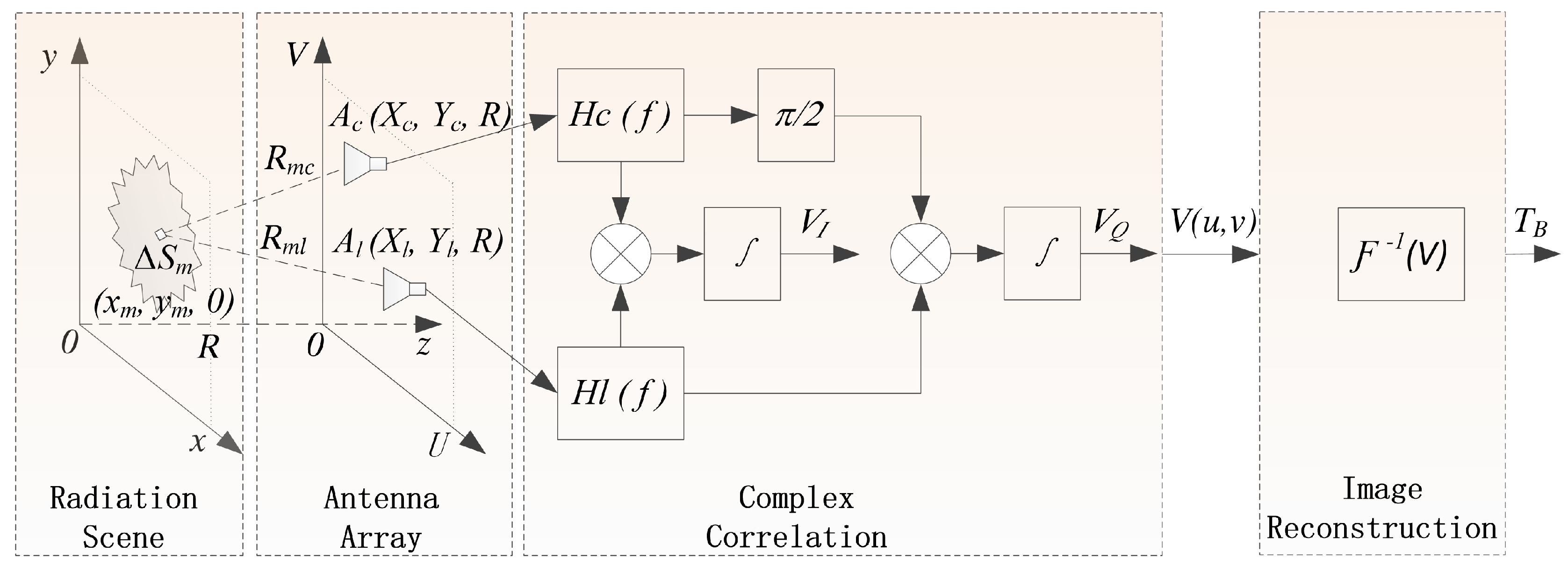
Figure 2.
Schematic diagram and illustration of non-local similar pixel grouping.
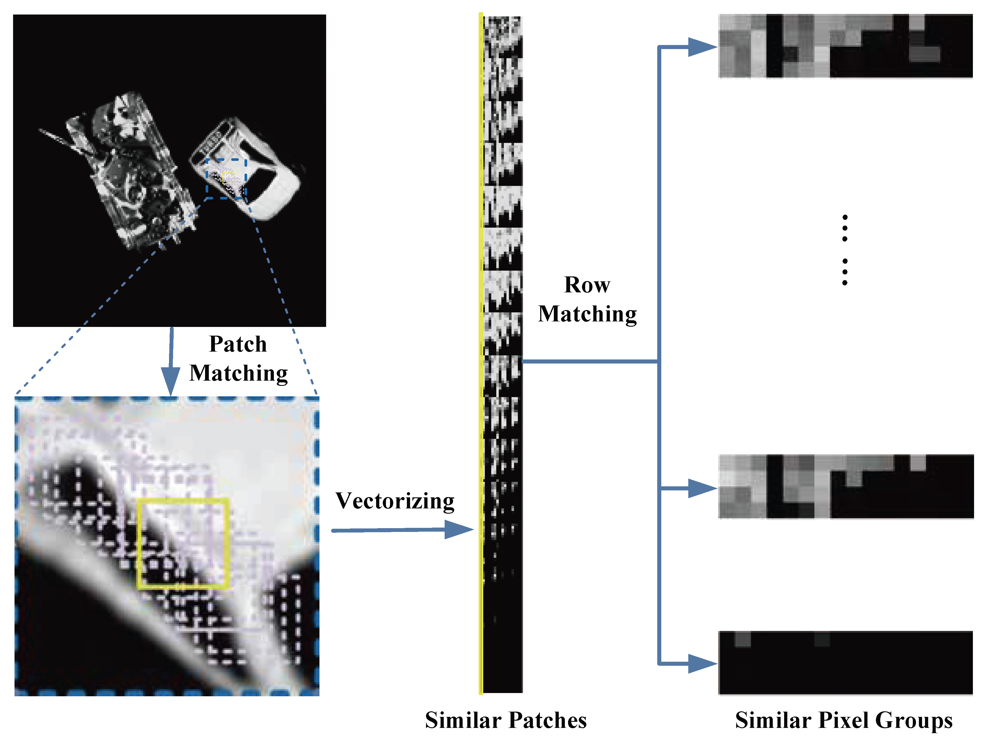
Figure 3.
Workflow of the InSAR-PNS reconstruction framework.
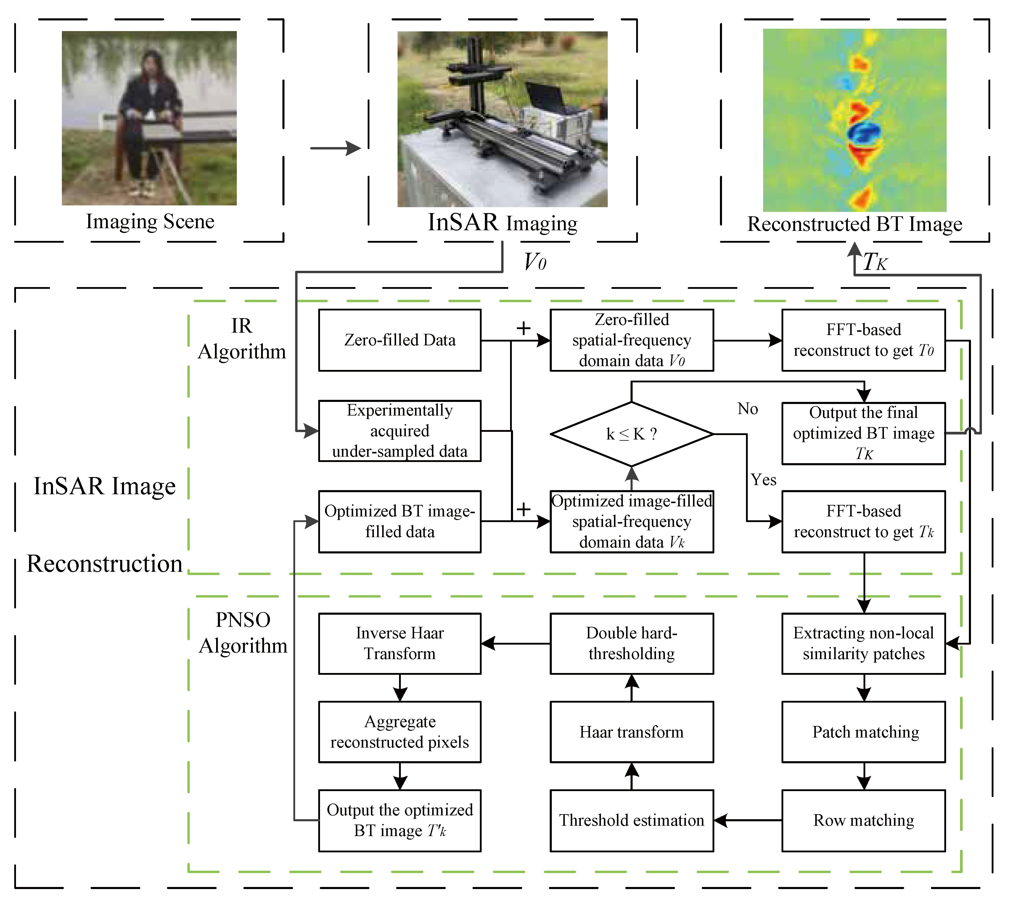
Figure 4.
Comparative reconstruction performance on simulated data: (a) Original simulated BT image; (b) MFFT reconstruction with full sampling; (c) CS reconstruction with 80% sampling; (d) Proposed InSAR-PNS reconstruction with 80% sampling.
Figure 4.
Comparative reconstruction performance on simulated data: (a) Original simulated BT image; (b) MFFT reconstruction with full sampling; (c) CS reconstruction with 80% sampling; (d) Proposed InSAR-PNS reconstruction with 80% sampling.
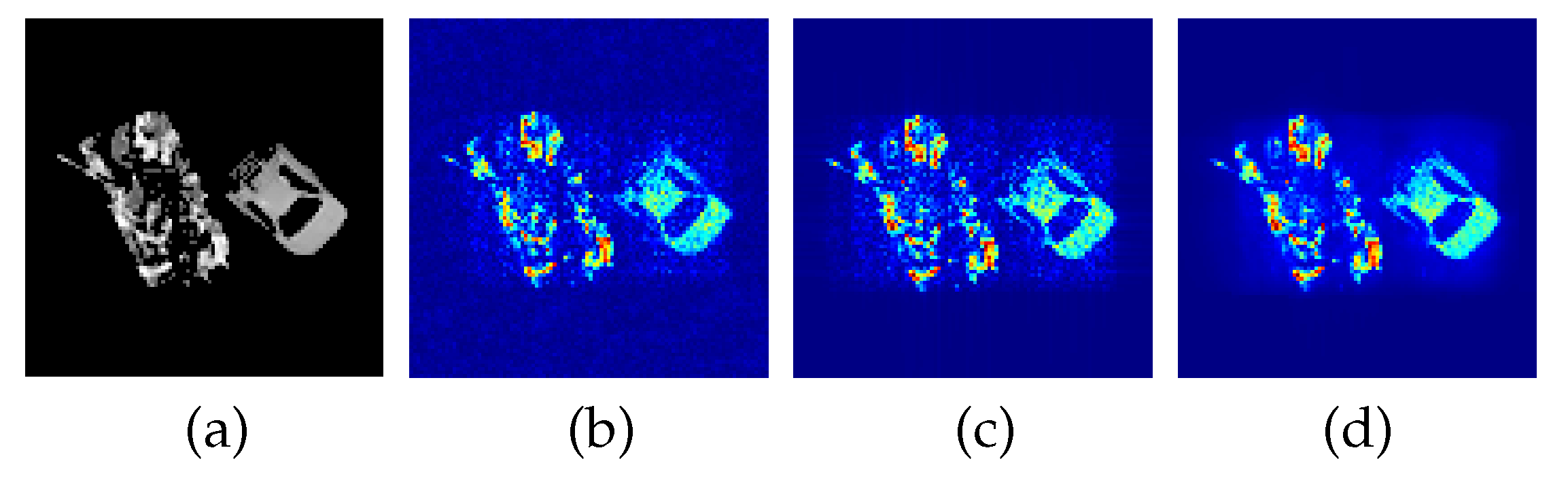
Figure 5.
Comparative reconstruction performance on simulated data: (a) Original simulated BT image; (b) MFFT reconstruction with full sampling; (c) CS reconstruction with 50% sampling; (d) Proposed InSAR-PNS reconstruction with 50% sampling.
Figure 5.
Comparative reconstruction performance on simulated data: (a) Original simulated BT image; (b) MFFT reconstruction with full sampling; (c) CS reconstruction with 50% sampling; (d) Proposed InSAR-PNS reconstruction with 50% sampling.
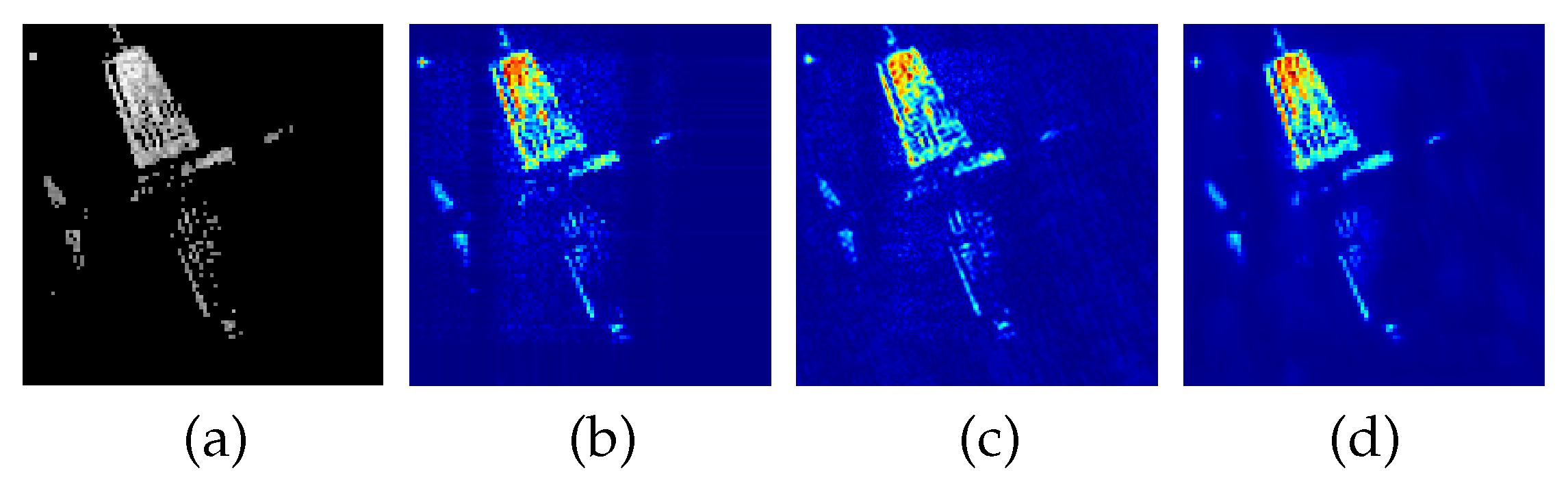
Figure 6.
Comparative reconstruction performance under simulated interference conditions: (a) MFFT, (b) CS, and (c) proposed InSAR-PNS with low-intensity interference; (d) MFFT, (e) CS, and (f) proposed InSAR-PNS with high-intensity interference.
Figure 6.
Comparative reconstruction performance under simulated interference conditions: (a) MFFT, (b) CS, and (c) proposed InSAR-PNS with low-intensity interference; (d) MFFT, (e) CS, and (f) proposed InSAR-PNS with high-intensity interference.
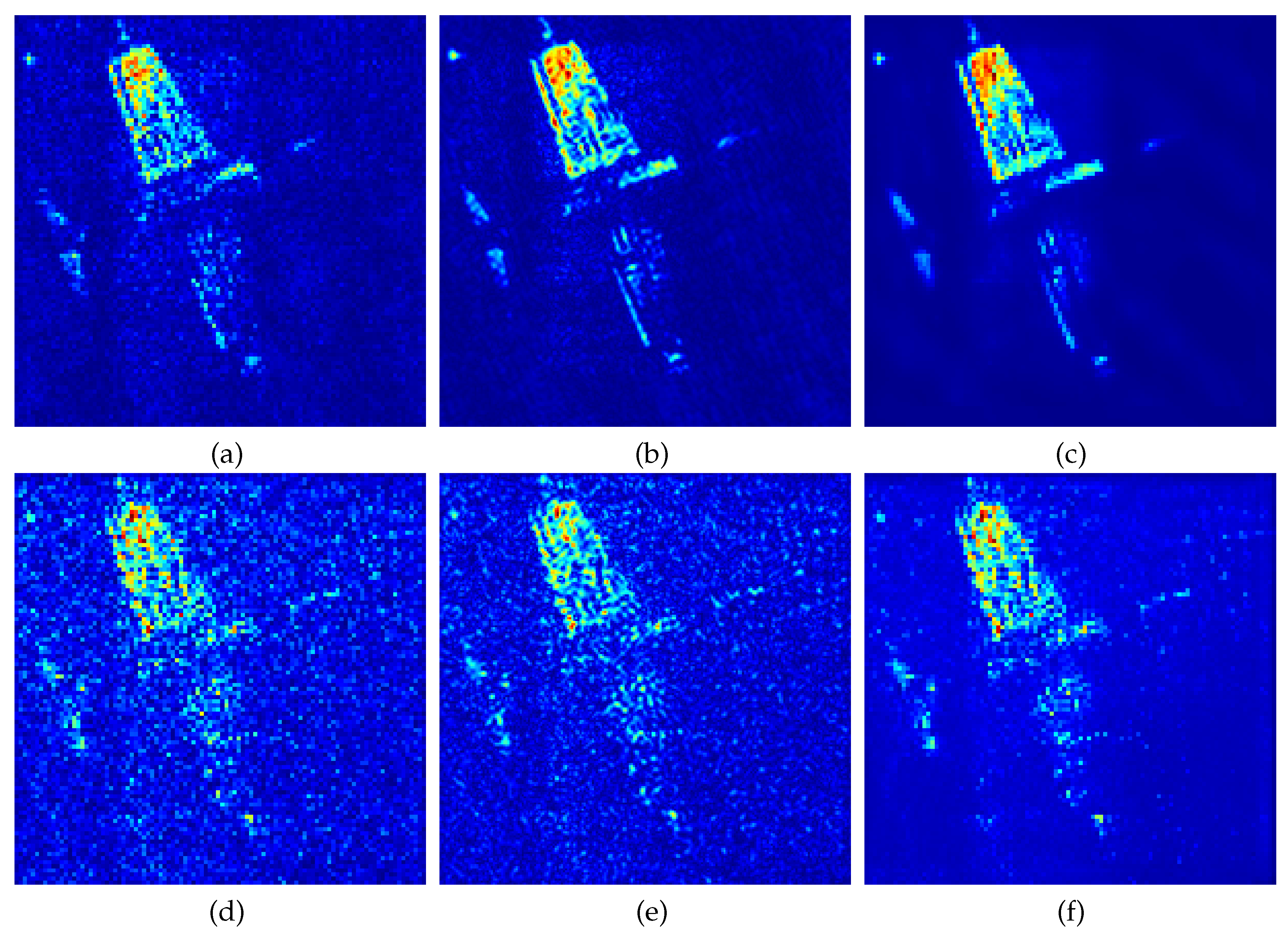
Figure 7.
Quantitative results (PSNR) of a comparative study on the simulation system. (a) PSNR performance of CS and InSAR-PNS with different sampling rate. (b) PSNR performance of MFFT, CS, and InSAR-PNS with different intensity levels of noise.
Figure 7.
Quantitative results (PSNR) of a comparative study on the simulation system. (a) PSNR performance of CS and InSAR-PNS with different sampling rate. (b) PSNR performance of MFFT, CS, and InSAR-PNS with different intensity levels of noise.
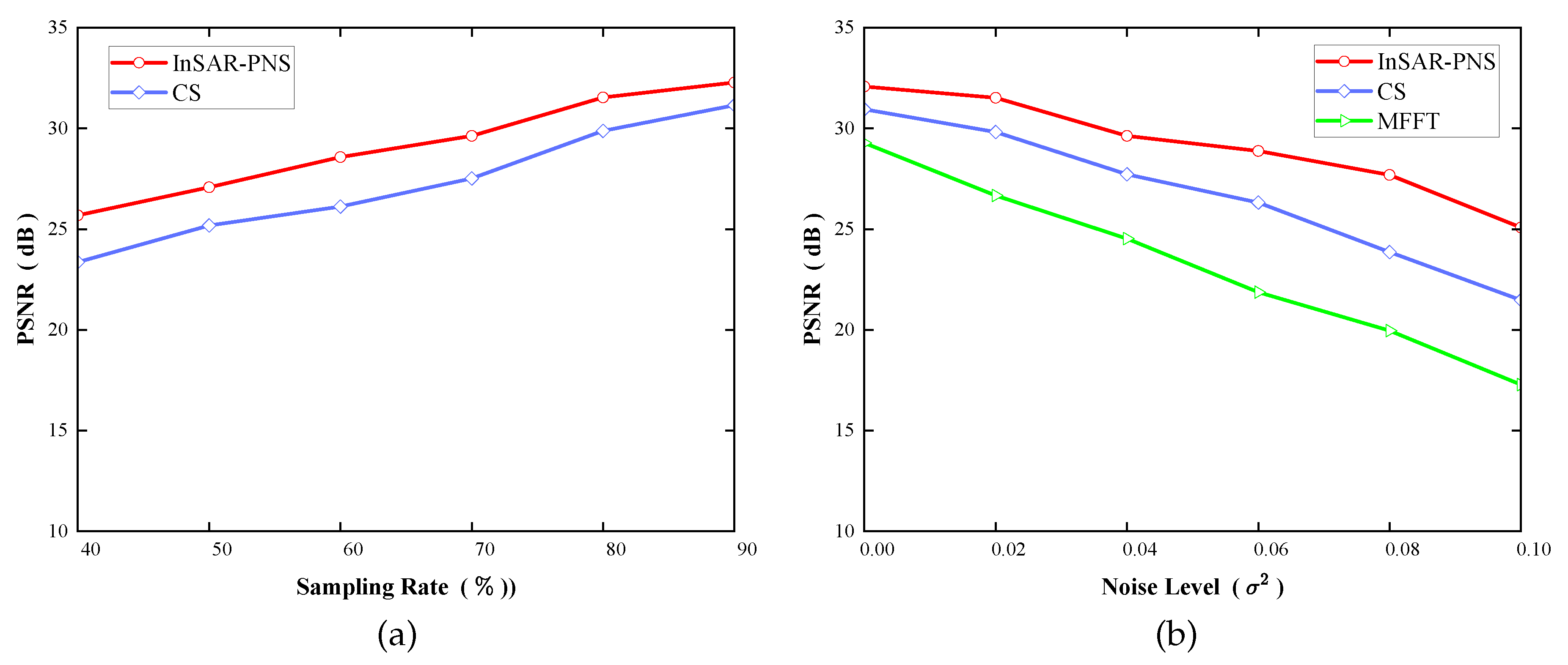
Figure 8.
100 GHz millimeter-wave InSAR imaging system. (a) Front view: T-shaped antenna array (b) Rear view: digital control units and host computer (c) Scene 1: vehicle target at 6 m (d) Scene 2: human carrying semi-concealed metal disk at 3.3 m
Figure 8.
100 GHz millimeter-wave InSAR imaging system. (a) Front view: T-shaped antenna array (b) Rear view: digital control units and host computer (c) Scene 1: vehicle target at 6 m (d) Scene 2: human carrying semi-concealed metal disk at 3.3 m
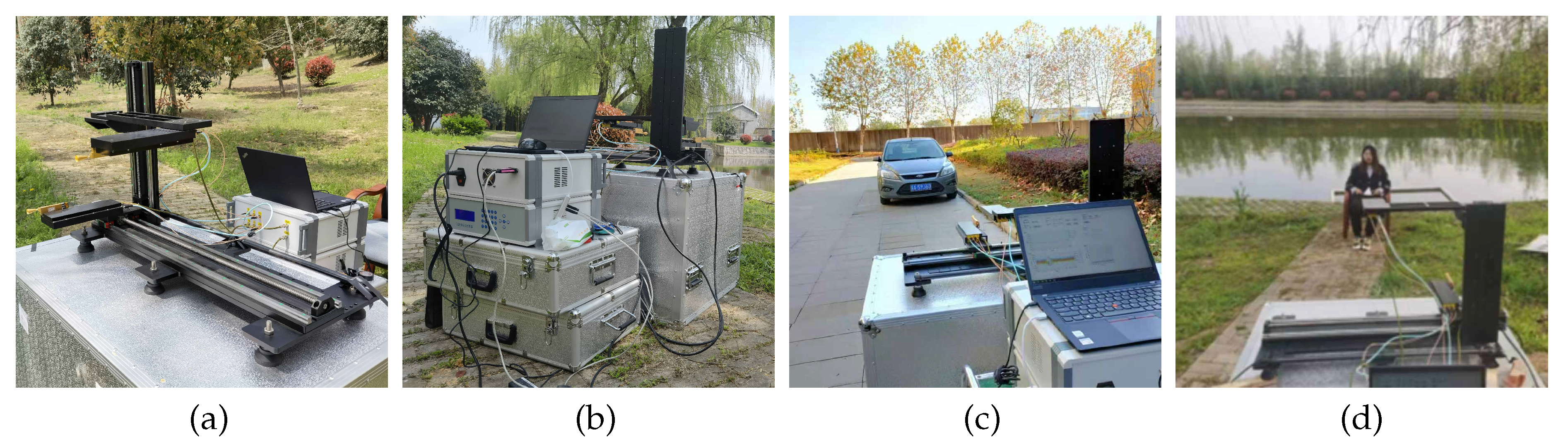
Figure 9.
Reconstruction performance under clear-sky conditions: (a) Reference optical image; (b) FFT reconstruction; (c) CS reconstruction; (d) Proposed InSAR-PNS reconstruction.
Figure 9.
Reconstruction performance under clear-sky conditions: (a) Reference optical image; (b) FFT reconstruction; (c) CS reconstruction; (d) Proposed InSAR-PNS reconstruction.
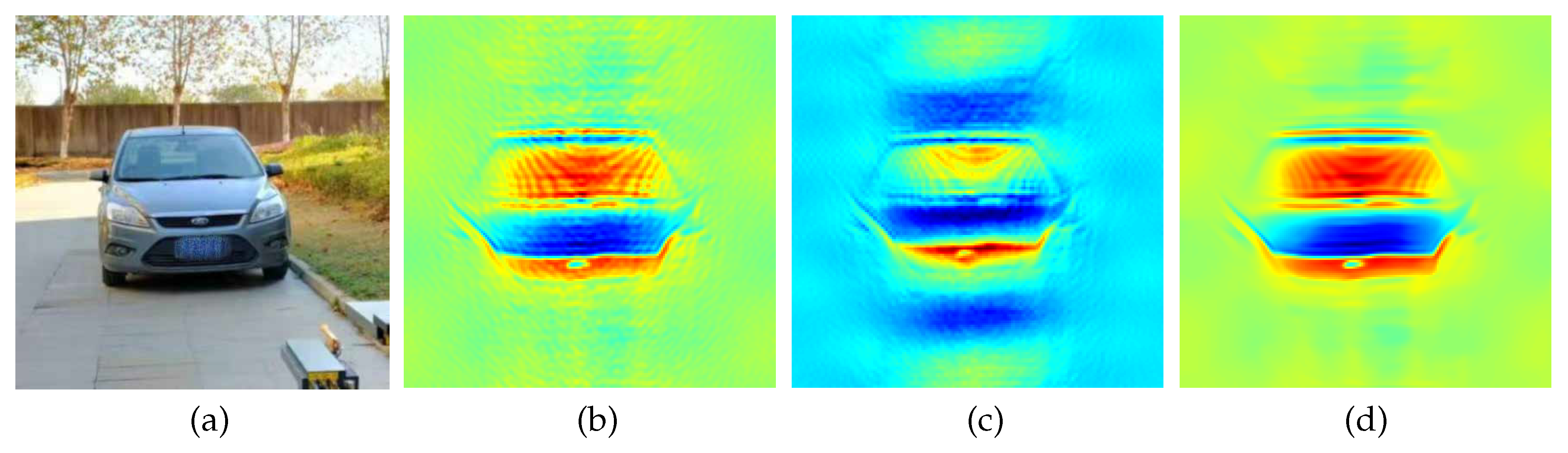
Figure 10.
Reconstruction performance under partly cloudy conditions with textile occlusion: (a) Reference optical image; (b) FFT reconstruction; (c) CS reconstruction; (d) Proposed InSAR-PNS reconstruction.
Figure 10.
Reconstruction performance under partly cloudy conditions with textile occlusion: (a) Reference optical image; (b) FFT reconstruction; (c) CS reconstruction; (d) Proposed InSAR-PNS reconstruction.
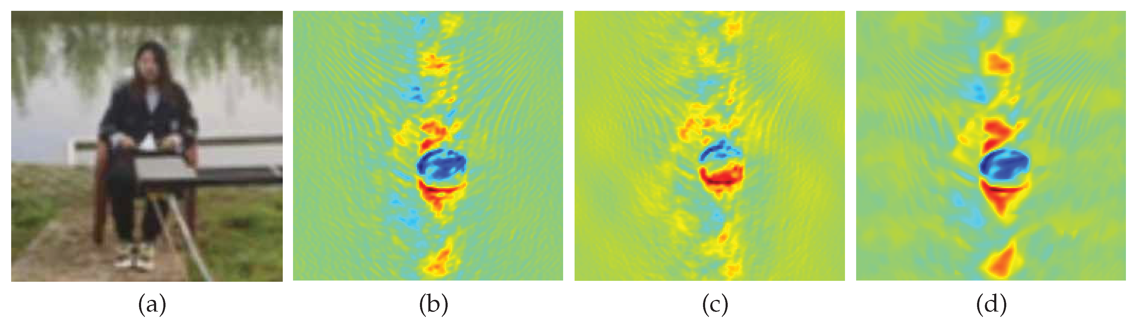

Table 1.
PNSO algorithm workflow.
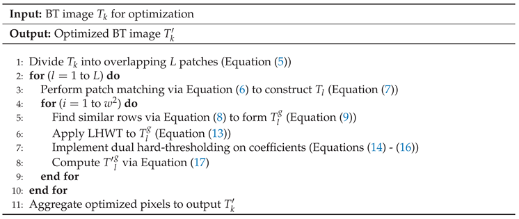 |
Table 2.
IR algorithm workflow.
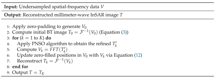 |
Table 3.
Parameter configuration of InSAR imaging simulation system.
| Simulation Parameters | FFT Reconstruction | CS and InSAR-PNS Reconstruction |
|---|---|---|
| Center frequency | 100GHz | 100GHz |
| Antenna array size | 100 x 100 | (90-40) x (90-40) |
| Receiver number | 150 | 135-60 |
| Inter-element spacing | 12mm | 12mm |
| Image distance | 6m | 6m |
| Image pixel size | 100 x 100 | 100 x 100 |
| image gray | 0-255 | 0-255 |
Table 4.
Main Parameters of the two-Element InSAR imaging system.
| System Parameter | Value |
|---|---|
| Operating Frequency | 100 GHz |
| Bandwidth | 1 GHz |
| Number of Antenna Elements | 2 |
| Field of View (FOV) | 20 ° |
| Angular Resolution | 0.3 ° |
| Temperature Sensitivity | 2K |
Disclaimer/Publisher’s Note: The statements, opinions and data contained in all publications are solely those of the individual author(s) and contributor(s) and not of MDPI and/or the editor(s). MDPI and/or the editor(s) disclaim responsibility for any injury to people or property resulting from any ideas, methods, instructions or products referred to in the content. |
© 2025 by the authors. Licensee MDPI, Basel, Switzerland. This article is an open access article distributed under the terms and conditions of the Creative Commons Attribution (CC BY) license (http://creativecommons.org/licenses/by/4.0/).
Copyright: This open access article is published under a Creative Commons CC BY 4.0 license, which permit the free download, distribution, and reuse, provided that the author and preprint are cited in any reuse.


