Submitted:
25 July 2025
Posted:
25 July 2025
You are already at the latest version
Abstract
Bandgap resonance is the significant structural response caused by the dynamic loads within the bandgap of a metamaterial. This phenomenon is undesirable because it undermines the vibration isolation performance of the metamaterial. The sufficient condition to avoid bandgap resonance is derived for stretch-dominated metamaterials, which are modelled as pin-jointed bar structures. Specifically, the metamaterials should exhibit spatial inversion symmetry and be subjected to certain boundary conditions. For metamaterials that satisfy this sufficient condition, the expected bandgaps can be obtained by adjusting the node coordinates and the element cross-sectional areas of the unit cell under symmetry constraint. A two-dimensional example is presented to validate the proposed sufficient condition and the corresponding design method.
Keywords:
stretch-dominated metamaterial
; mechanical metamaterial
; bandgap
; bandgap resonance
; structure design
1. Introduction
Owing to the ability to isolate mechanical waves within specific frequency ranges, bandgap mechanical metamaterials are broadly applicable in engineering vibration and sound insulation. Vasconcelos et al. [1] proposed a metamaterial-based interface to attenuate pressure waves induced by the impact hammer acting on the top of an offshore monopile. Zuo et al. [2] applied a star-shaped metamaterial to the shell of an underwater vehicle to reduce engine noise emission. A lattice-structured metamaterial capable of both sound insulation and ventilation was developed by Li et al. [3], and can be used as a roadside noise barrier. Seismic metamaterials composed of periodically arranged building foundations have been validated for shielding seismic waves and train-induced vibrations [4]. Replacing conventional aggregates with local resonant masses [5] enables concrete structural members to function as metamaterials capable of dissipating elastic waves induced by dynamic loads.
Dynamic loads within the bandgap may still induce significant structural responses in the metamaterials, which is known as bandgap resonance [6]. For example, Zhang et al. [7] designed a negative stiffness metamaterial that exhibits a peak in its frequency response curve within the bandgap range. Jiang et al. [8] designed negative stiffness metamaterials whose frequency response curves do not exactly match their bandgaps. The chiral and hexagonal lattices proposed by Li et al. [9,10] also experience large frequency responses within the bandgap ranges. Bandgap resonance can similarly be observed in the frequency response curves of the metamaterials studied in Ref. [11,12,13,14]. The presence of bandgap resonance suggests that certain eigenfrequencies of the metamaterial lie within the bandgap range, thereby compromising its vibration isolation performance. Therefore, it is necessary to prevent this phenomenon in the engineering design of bandgap metamaterials.
Bandgap resonance attracted early attention in the field of solid-state physics. In calculating the specific heat capacity of crystals, periodically arranged atoms are modelled as vibrating one-dimensional atomic chains. Thus, some early studies focused on the correspondence between the eigenfrequency spectra and the dispersion functions of finite atomic chains. Born [15] studied two types of one-dimensional atomic chains and concluded that the spectrum of a finite atomic chain with free ends is consistent with its dispersion function. Wallis [16], however, identified an eigenfrequency within the bandgap while analyzing the spectrum of a finite diatomic chain. Since then, similar phenomena have been widely observed in elastomers [17,18,19,20].
Calculating the dispersion function via Bloch’s theorem assumes that the metamaterials exhibit translational symmetry [21], necessitating that they be either infinitely extended or subjected to periodic boundary conditions [22]. However, finite metamaterials in engineering possess non-periodic boundaries, so their spectra deviate from the dispersion functions. This suggests that the existence of bandgap resonance is determined by the boundary conditions. Bastawrous et al. [6] introduced boundary conditions as perturbations to the dynamic stiffness matrix and analytically derived a closed-form condition for the existence of bandgap resonance in finite diatomic chains. Guo et al. [23] and Sugino et al. [24] solved dynamic differential equations with boundary conditions substituted to obtain the spectra of finite two-phase plates. Jin et al. [25] incorporated boundary conditions in the form of a Fourier series into the dynamic stiffness matrix and solved the spectrum of a two-phase metamaterial plate. By comparing the obtained spectra with the dispersion functions of the metamaterials, the existence of bandgap resonance can be identified.
Analytical calculations of the spectra of metamaterials require explicit expressions for the eigenfrequencies, which poses a substantial mathematical challenge. As a result, existing studies have primarily focused on simple systems, such as two-phase plates or diatomic chains [6,23,24,25]. However, metamaterials designed for specific bandgaps are usually complex, making it difficult to analytically solve their spectra. Therefore, to ensure the vibration isolation performance of a designed metamaterial, bandgap resonance should preferably be avoided without solving the spectrum.
This paper proposes a design method for stretch-dominated metamaterials that achieve expected bandgaps while avoiding bandgap resonance. The paper is organized as follows: Section 2 derives the sufficient condition for avoiding the bandgap resonance in stretch-dominated metamaterials. Section 3 presents the equations for designing the unit cell parameters under symmetry constraint. A design example is illustrated in Section 4, which is used to validate both the sufficient condition and the corresponding design method. Finally, Section 5 draws some conclusions.
2. Sufficient Condition for Avoiding Bandgap Resonance
A two-dimensional stretch-dominated metamaterial is used as an example to demonstrate the derivation of the sufficient condition for avoiding bandgap resonance. As shown in Figure 1, a 3×3 metamaterial, denoted by m, is modelled as a pin-jointed bar structure and subjected to a boundary condition that can be practically realized in engineering. Figure 2a and Figure 3a show the distributions of modal forces and displacements on the boundaries corresponding to any eigenfrequency ωj of m. Except for the corner nodes, the horizontal components of the node forces are zero on the top and bottom edges, while the vertical components are zero on the left and right edges. Similarly, the vertical components of the node displacements are zero on the top and bottom edges, and the horizontal components are zero on the left and right edges. Thus, it can be derived that
where dt/b and ft/b are the displacement and force vectors of the nodes on the top or bottom edge; dl/r and fl/r are the displacement and force vectors of the nodes on the left or right edge; and (u=1, …, nt/b) are the x and y components of the displacement of the u-th node on the top or bottom edge, respectively, and (u=1, …, nt/b) are the corresponding force components; and (u=1, …, nl/r) are the x and y components of the displacement of the u-th node on the left or right edge, and (u=1, …, nl/r) are the corresponding force components; nt/b is the number of nodes on the top or bottom edge, and nl/r is that on the left or right edge; the superscript T denotes the transpose of a vector or matrix.
Spatial inversion of m in the x-direction (i.e., mirroring across the y-axis) yields the metamaterial mx. The distributions of modal forces and displacements on the boundaries are shown in Figure 2b and Figure 3b, and the corresponding frequency remains constant at ωj. According to Figure 2b and Figure 3b, the boundary node displacement and force vectors of mx can be written as
Spatial inversion of m in the y-direction (i.e., mirroring across the x-axis) yields the metamaterial my. The distributions of modal forces and displacements on the boundaries are shown inFigure 2c and Figure 3c, and the corresponding frequency remains constant at ωj. According to Figure 2c and Figure 3c, the boundary node displacement and force vectors of my can be written as
Spatial inversion of mx in the y-direction yields the metamaterial mxy. The distributions of modal forces and displacements on the boundaries are shown in Figure 2d and Figure 3d, and the corresponding frequency remains constant at ωj. According to Figure 2d and Figure 3d, the boundary node displacement and force vectors of mxy can be written as
As can be seen from Figure 2 and Eqs. (1), (2), (5), (6), (9), (10), (13) and (14), the boundary node displacement vectors satisfy
Moreover, Figure 3 and Eqs. (3), (4), (7), (8), (11), (12), (15) and (16) indicate that the boundary node force vectors satisfy the following relationships except for corner nodes:
Let nodes 1, 2, 3 and 4 denote the lower right corner node of m, the lower left corner node of mx, the upper right corner node of my, and the upper left corner node of mxy, respectively. Then, their node forces satisfy
Eqs. (17)– (19) indicate that the corresponding nodes on the bottom edge of m and the top edge of my have identical displacements, and their node forces are in equilibrium. The same relationship holds between the right edge of m and the left edge of mx, the top edge of mxy and the bottom edge of mx, and the right edge of my and the left edge of mxy. This suggests that m, mx, my, and mxy can be merged into a new structure M. Figure 4a and Figure 4b show the distributions of its modal forces and displacements on the boundaries, and the corresponding frequency is still ωj.
The boundary node displacement and force vectors of M can be written as
According to Eqs. (20)– (27), the node displacements and forces on the boundaries of M satisfy the periodic boundary condition [26]. However, M may not be a translationally symmetric metamaterial because m is not necessarily identical to mx, my and mxy. Conversely, if m remains unchanged after the spatial inversions in both the x- and y-directions, M is a metamaterial satisfying the periodic boundary condition. This requires that the unit cell of m exhibits spatial inversion symmetry along x- and y-axes. In this case, the spectrum of M must coincide with the dispersion function obtained via Bloch’s theorem, indicating that none of the eigenfrequencies of M, including ωj, lie within the bandgap. Since any eigenfrequency ωj of m lies outside the bandgap, the metamaterial m can avoid bandgap resonance.
The above derivation can be generalized to three-dimensional metamaterials and some other boundary conditions. For two- and three-dimensional cases, the applicable boundary conditions are listed in Table 1 and Table 2, respectively.
In Table 1 and Table 2, x, y and z represent nodes on the boundaries normal to the x-, y- and z-directions, respectively; c1, c2 and c3 represent constraints applied in the x-, y- and z- directions, respectively.
In summary, the sufficient condition for avoiding bandgap resonance can be express as
3. Perturbation of Bandgap
The following generalized characteristic equation [26,27,28,29] can be used to solve the dispersion function of the metamaterial consisting of unit cells with spatial inversion symmetry:
where ; and are the d·n×d·n stiffness and mass matrices of the unit cell, respectively, and their explicit forms can be found in Ref. [29]; n is the number of nodes in the unit cell; the superscript H denotes the Hermite transpose; is the d·n×d·r reduction matrix introducing Bloch’s theorem [29], and r is the number of inequivalent nodes [29]; ω(k) is the circular frequency, and k is the d×1 wave vector [30]. Once k is given, the generalized eigenvalues ωj(k)2 (j=1, 2, …, d·r) and their corresponding eigenvectors (d·r×1) can be solved via Eq. (28). Thus, the dispersion function of the metamaterial, i.e., the k‒ω relation, is established with a total of d·r branches of k‒ωj.
According to matrix perturbation theory [28,29], the perturbation of branch j caused by the increments of unit cell parameters, including node coordinates and element cross-sectional areas, can be calculated by
where is the (b+d·n)×1 incremental unit cell parameter vector; b is the number of elements in the unit cell; Ai (i=1,…, b) is the cross-sectional area of the i-th element; ( p=1, …, n, k=1, .., d) is the k-th coordinate of the p-th node. Oj(k) is a 1×(b+d·n) row vector whose v-th component is
where v=b+d·(p-1)+k for the second term; is the eigenvector normalized by ; , . The explicit forms of ,, and are given in Ref. [29].
An illustrative bandgap between the lower branch ωl(k) and the upper branch ωu(k) is shown in Figure 5. The range of the bandgap is [ωl(kl), ωu(ku)], where kl and ku are the wave vectors corresponding to the maximum value of ωl(k) and the minimum value of ωu(k), respectively. Substituting kl and ku into Eq. (29), the perturbation of ωl(kl) and ωu(ku) can be expressed as
The difference between the expected bandgap [ωl, ωu] shown in Figure 5 and the current bandgap is Δωt={ωu-ωu(ku), ωl-ωl(kl)}T. By substituting Δωt into Eq. (31), Δε for adjusting unit cell parameters and tuning bandgap can be solved. However, Δε must satisfy spatial inversion symmetry, or it will break the symmetry of the unit cell. Figure 6 shows a unit cell with 8 nodes and 12 elements. An increment vector adjusting the coordinates of nodes 5, 6, 7 and 8 with , , and satisfies spatial inversion symmetry, and is denoted as Δεg. Similarly, ΔA5=1, ΔA6=1, ΔA7=1 and ΔA8=1 can be assembled into another Δεg satisfying spatial inversion symmetry. If there are at most τ linearly independent Δεg, then any incremental unit cell parameter vector satisfying spatial inversion symmetry can be expressed as
where Δκ is an arbitrary τ×1 coefficient vector.
Substituting Eq. (32) and Δωt into Eq. (31), it can be obtained that
The least squares solution [31] of Eq. (33) is
By substituting Eq. (34) into Eq. (32), the resulting Δεsym can be used to adjust the unit cell parameters and tune the bandgap under the constraint of spatial inversion symmetry.
The unit cell parameters should be modified in small steps due to the strong nonlinearity in their relationship with the dispersion function. Thus, Δεsym is scaled by
where s is a specified scaling factor; ||•|| denotes the 2-norm of the vector. The expected bandgap can be obtained by iteratively adjusting the unit cell parameters with Δεs until ||Δωt|| falls below a specified tolerance c.
4. Example
Figure 7a shows a square unit cell with a side length of 10 mm that exhibits spatial inversion symmetry along the x- and y-axes. The origin of the coordinate system is at the center of the unit cell with the axes shown in Figure 7a. The node coordinates are listed in Table 3. All the elements of the unit cell have a circular cross-section with a radius of 0.3 mm (area A=0.283 mm2) and are made of plastic with a Young’s modulus of E=1.2 GPa and a density of ρ=0.9 g/cm3.
For this unit cell, the dispersion function obtained using Eq. (28) consists of 52 branches, whose significant overlap makes it difficult to depict their surfaces on a plane. To illustrate the band structure, a frequency distribution function for branch j can be constructed as follows:
where Π denotes the first Brillouin zone [30]; dA=dkxdky is the area of the infinitesimal element of Π; and kx and ky are the x and y components of k, respectively. According to Eq. (36), Dj(ω) represents the total area of the infinitesimal elements for which ωj=ω. If Dj(ω)≠0, there must exist a wave vector k such that ωj(k)=ω. Therefore, ωj(k) lies within the frequency domain with nonzero Dj(ω). The frequency distribution of the dispersion function can be visualized by plotting Dj(ω) for all branches, with ω as the horizontal axis and area as the vertical axis. Figure 7b shows 27 lower-frequency branches distributed between 0 and 3100 Hz.
This example aims to achieve a bandgap of 600–1000 Hz by designing the coordinates of nodes 5–29 and the cross-sectional areas of all elements. According to Figure 7b, the expected bandgap is most likely generated between branches 3 and 4. The unit cell parameters are iteratively adjusted using Eqs. (31)– (35) with a tolerance of c=2. The resulting unit cell is shown in Fib. 8a, whose element cross-sectional areas and node coordinates are listed in Table 4 and Table 5, respectively. The frequency distribution of the updated dispersion function is shown in Figure 8b, where a bandgap of 600.0–998.6 Hz can be found.
A metamaterial consisting of 4×4 designed unit cells is shown in Figure 9a. The metamaterial is denoted as PBC, FBC or SBC when the periodic, free, or specific boundary condition is imposed. The specific boundary condition is illustrated in Figure 9b and corresponds to case 3 in Table 1. In addition, the symmetry of the designed unit cell can be slightly broken by adjusting the coordinate of node 15 to (-4.03, 1.00), resulting in a bandgap of 601.0–904.7 Hz. The 4×4 metamaterial, consisting of this asymmetric unit cell and subjected to the specific boundary condition, is denoted as SBCA.
The eigenfrequencies and frequency-response curves of PBC, FBC, SBC, and SBCA are shown in Figure 10, Figure 11, Figure 12 and Figure 13. The frequency-response function is defined as
where ||din(ω)|| is the displacement amplitude at input node 1, and ||dout(ω)|| is that at output node 2 or 3. These nodes are labeled in Figure 9a. With a modal damping of 0.02, ||din(ω)|| and ||dout(ω)|| are calculated using the modal superposition method (MS) [32] and the finite element software ANSYS, respectively. The MS is implemented in MATLAB, and the procedure includes the following steps: (1) Set up the dynamic equation for the metamaterial consisting of 4×4 unit cells. (2) Calculate the eigenfrequencies and eigenmodes of the metamaterial. (3) Calculate the displacements at the input and output nodes, i.e., din and dout, under a simple harmonic load using the displacement equation [32] of the modal superposition method. The metamaterials are also modelled in ANSYS. All the elements are simulated by Link180. A harmonic response analysis is conducted to obtain the displacements din and dout, with the solution method [33] set to FULL.
As illustrated in Figure 10, the eigenfrequencies and frequency-response curves of PBC are consistent with the bandgap, confirming that the metamaterial with expected bandgap has been successfully designed. However, when the metamaterial is subjected to the free boundary condition, eigenfrequencies emerge within the bandgap, as illustrated in Figure 11. Figure 12 shows that the bandgap resonances in SBC are effectively suppressed by imposing the specific boundary condition, thereby validating the second condition of Theorem 1. For the asymmetric metamaterial, even when the specific boundary condition is imposed, bandgap resonances still emerge in the frequency-response curves of Figure 13. This validates the first condition of Theorem 1.
5. Conclusions
This paper proposes a design method for stretch-dominated metamaterials that achieve expected bandgaps while avoiding bandgap resonance. The conclusions are summarized as follows:
(1) A d-dimensional metamaterial can avoid bandgap resonance if both of the following conditions are satisfied: 1. The unit cell exhibits spatial inversion symmetry along all d coordinate axes; 2. One of the boundary conditions listed in Table 1 and Table 2is imposed.
(2) The perturbation expression of the bandgap is derived. By introducing symmetry constraint, the incremental unit cell parameter vector can be solved via this perturbation expression. This vector is then used to adjust the node coordinates and element cross-sectional areas to tune the bandgap.
(3) A two-dimensional metamaterial example is used to validate the proposed sufficient condition and design method. The designed metamaterial, which satisfies spatial inversion symmetry and the boundary condition in Table 1, achieves the expected bandgap and avoids bandgap resonance, thus validating the proposed design method. However, bandgap resonances emerge once either of these two conditions is not satisfied. This validates the sufficient condition for avoiding bandgap resonance.
Author Contributions
Conceptualization, Methodology, Software, Validation, Formal Analysis, Investigation, Resources, Data Curation, Writing – Original Draft Preparation, Writing – Review & Editing, Visualization, Supervision: Zijian Wang
Funding
This research received no external funding.
Data Availability Statement
The raw data supporting the conclusions of this article will be made available by the authors on request.
Acknowledgments
Sincere thanks to Professor Deng Hua for the guidance on my research during my graduate studies.
Conflicts of Interest
The author declares no conflicts of interest.
References
- Azevedo Vasconcelos, A.C.; Valiya Valappil, S.; Schott, D.; Jovanova, J.; Aragón, A.M. A Metamaterial-Based Interface for the Structural Resonance Shielding of Impact-Driven Offshore Monopiles. Eng. Struct. 2024, 300, 117261. [Google Scholar] [CrossRef]
- Zuo, Y.; Yang, D.; Zhuang, Y. Broadband Transient Vibro-Acoustic Prediction and Control for the Underwater Vehicle Power Cabin with Metamaterial Components. Ocean. Eng. 2024, 298, 117121. [Google Scholar] [CrossRef]
- Li, X.; Zhao, M.; Yu, X.; Wei Chua, J.; Yang, Y.; Lim, K.M.; Zhai, W. Multifunctional and Customizable Lattice Structures for Simultaneous Sound Insulation and Structural Applications. Mater. Design. 2023, 234, 112354. [Google Scholar] [CrossRef]
- Zheng, H.; Miao, L.; Xiao, P.; Lei, K.; Wang, Q. Novel Metamaterial Foundation with Multi Low-Frequency Bandgaps for Isolating Earthquakes and Train Vibrations. Structures. 2024, 61, 106070. [Google Scholar] [CrossRef]
- Mitchell, S.J.; Pandolfi, A.; Ortiz, M. Metaconcrete: Designed Aggregates to Enhance Dynamic Performance. J. Mech. Phys. Solids. 2014, 65, 69–81. [Google Scholar] [CrossRef]
- Bastawrous, M.V.; Hussein, M.I. Closed-Form Existence Conditions for Bandgap Resonances in a Finite Periodic Chain under General Boundary Conditions. J. Acoust. Soc. Am. 2022, 151, 286–298. [Google Scholar] [CrossRef]
- Zhang, K.; Qi, L.; Zhao, P.; Zhao, C.; Deng, Z. Buckling Induced Negative Stiffness Mechanical Metamaterial for Bandgap Tuning. Compos. Struct. 2023, 304, 116421. [Google Scholar] [CrossRef]
- Jiang, T.; Han, Q.; Li, C. Design and Compression-Induced Bandgap Evolution of Novel Polygonal Negative Stiffness Metamaterials. Int. J. Mech. Sci. 2024, 261, 108658. [Google Scholar] [CrossRef]
- Li, X.; Cheng, S.; Wang, R.; Yan, Q.; Wang, B.; Sun, Y.; Yan, H.; Zhao, Q.; Xin, Y. Design of Novel Two-Dimensional Single-Phase Chiral Phononic Crystal Assembly Structures and Study of Bandgap Mechanism. Results. Phys. 2023, 48, 106431. [Google Scholar] [CrossRef]
- Li, X.; Cheng, S.; Yang, H.; Yan, Q.; Wang, B.; Xin, Y.; Sun, Y.; Ding, Q.; Yan, H.; Li, Y.; Zhao, Q. Integrated Analysis of Bandgap Optimization Regulation and Wave Propagation Mechanism of Hexagonal Multi-Ligament Derived Structures. Eur. J. Mech. A-Solid. 2023, 99, 104952. [Google Scholar] [CrossRef]
- Yang, H.; Cheng, S.; Li, X.; Yan, Q.; Wang, B.; Xin, Y.; Sun, Y.; Ding, Q.; Yan, H.; Zhao, Q. Propagation Mechanism of Low-Frequency Elastic Waves and Vibrations in a New Tetragonal Hybrid Metamaterial. Int. J. Solids. Struct. 2023, 285, 112536. [Google Scholar] [CrossRef]
- Cheng, S.; Yang, H.; Yan, Q.; Wang, B.; Sun, Y.; Xin, Y.; Ding, Q.; Yan, H.; Wang, L. Study on the Band Gap and Directional Wave Propagation Mechanism of Novel Single-Phase Metamaterials. Physica. B. 2023, 650, 414545. [Google Scholar] [CrossRef]
- Yao, D.; Xiong, M.; Luo, J.; Yao, L. Flexural Wave Mitigation in Metamaterial Cylindrical Curved Shells with Periodic Graded Arrays of Multi-Resonator. Mech. Syst. Signal. Pr. 2022, 168, 108721. [Google Scholar] [CrossRef]
- Ruan, H.; Hou, J.; Li, D. Wave Propagation Characterization of 2D Composite Chiral Lattice Structures with Circular Plate Inclusions. Eng. Struct. 2022, 264, 114466. [Google Scholar] [CrossRef]
- Born, M. Lattice Dynamics and X-Ray Scattering. Proc. Phys. Soc. 1942, 54, 362. [Google Scholar] [CrossRef]
- Wallis, R.F. Effect of Free Ends on the Vibration Frequencies of One-Dimensional Lattices. Phys. Rev. 1957, 105, 540. [Google Scholar] [CrossRef]
- Hladky-Hennion, A.-C.; Allan, G.; de Billy, M. Localized Modes in a One-Dimensional Diatomic Chain of Coupled Spheres. J. Appl. Phys. 2005, 98. [Google Scholar] [CrossRef]
- Hladky-Hennion, A.-C.; Billy, M. de Experimental Validation of Band Gaps and Localization in a One-Dimensional Diatomic Phononic Crystal. J. Acoust. Soc. Am. 2007, 122, 2594–2600. [Google Scholar] [CrossRef]
- Hvatov, A.; Sorokin, S. Free Vibrations of Finite Periodic Structures in Pass- and Stop-Bands of the Counterpart Infinite Waveguides. J. Sound. Vib. 2015, 347, 200–217. [Google Scholar] [CrossRef]
- Al Ba’ba’a, H.; Nouh, M.; Singh, T. Pole Distribution in Finite Phononic Crystals: Understanding Bragg-Effects through Closed-Form System Dynamics. J. Acoust. Soc. Am. 2017, 142, 1399–1412. [Google Scholar] [CrossRef] [PubMed]
- Huang, K. Solid State Physics; Higher Education Press: Beijing, China, 1988. [Google Scholar]
- Hussein, M.I.; Leamy, M.J.; Ruzzene, M. Dynamics of Phononic Materials and Structures: Historical Origins, Recent Progress, and Future Outlook. Appl. Mech. Rev. 2014, 66. [Google Scholar] [CrossRef]
- Guo, Z.; Sheng, M.; Pan, J. Effect of Boundary Conditions on the Band-Gap Properties of Flexural Waves in a Periodic Compound Plate. J. Sound. Vib. 2017, 395, 102–126. [Google Scholar] [CrossRef]
- Sugino, C.; Ruzzene, M.; Erturk, A. An Analytical Framework for Locally Resonant Piezoelectric Metamaterial Plates. Int. J. Solids. Struct. [CrossRef]
- Jin, G.; Zhang, C.; Ye, T.; Zhou, J. Band Gap Property Analysis of Periodic Plate Structures under General Boundary Conditions Using Spectral-Dynamic Stiffness Method. Appl. Acoust. 2017, 121, 1–13. [Google Scholar] [CrossRef]
- Phani, A.S.; Woodhouse, J.; Fleck, N.A. Wave Propagation in Two-Dimensional Periodic Lattices. J. Acoust. Soc. Am. 2006, 119, 1995–2005. [Google Scholar] [CrossRef]
- Messner, M.C.; Barham, M.I.; Kumar, M.; Barton, N.R. Wave Propagation in Equivalent Continuums Representing Truss Lattice Materials. Int. J. Solids. Struct. 74. [CrossRef]
- Chen, S. Matrix Perturbation Theory in Structural Dynamic Design, Science Press: Beijing, China, 1999.
- Wang, Z.; Deng, H.; Liu, H. A Matrix Method for Designing Bandgap of Stretch-Dominated Mechanical Metamaterials. J. Sound. Vib. 2025, 617, 119257. [Google Scholar] [CrossRef]
- Grosso, G.; Parravicini, G.P. Solid State Physics; Elsevier: Amsterdam, Netherlands, 2000. [Google Scholar]
- Ben-Israel, A.; Greville, T.N.E. Generalized Inverses: Theory and Applications; Springer Science & Business Media, 2003; ISBN 978-0-387-00293-4.
- Chopra, A.K. Dynamics of Structures; Pearson Education: London, UK, 2007. [Google Scholar]
- 16.1.11.1. Coupled Field Harmonic, Harmonic Acoustics, and Harmonic Response Options Available online:. Available online: https://ansyshelp.ansys.com/public/account/secured?returnurl=/Views/Secured/corp/v242/en/wb_sim/ds_options_harmonic.html?q=hropt (accessed on 8 March 2025).
Figure 1.
A 3×3 metamaterial with specific boundary condition.
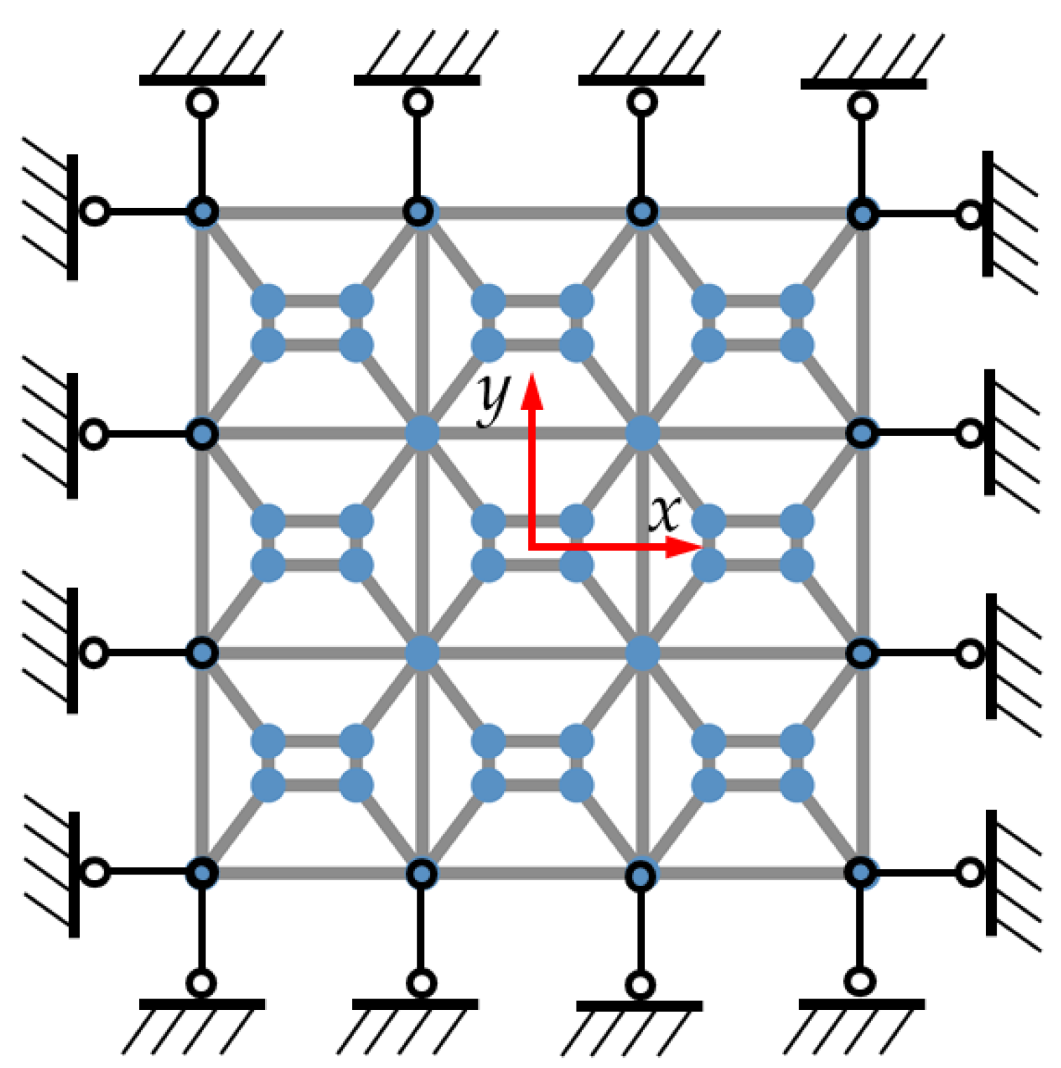
Figure 2.
Distributions of modal forces on the boundaries of 3×3 metamaterials: (a) m; (b) mx; (c) my; (d) mxy;.
Figure 2.
Distributions of modal forces on the boundaries of 3×3 metamaterials: (a) m; (b) mx; (c) my; (d) mxy;.
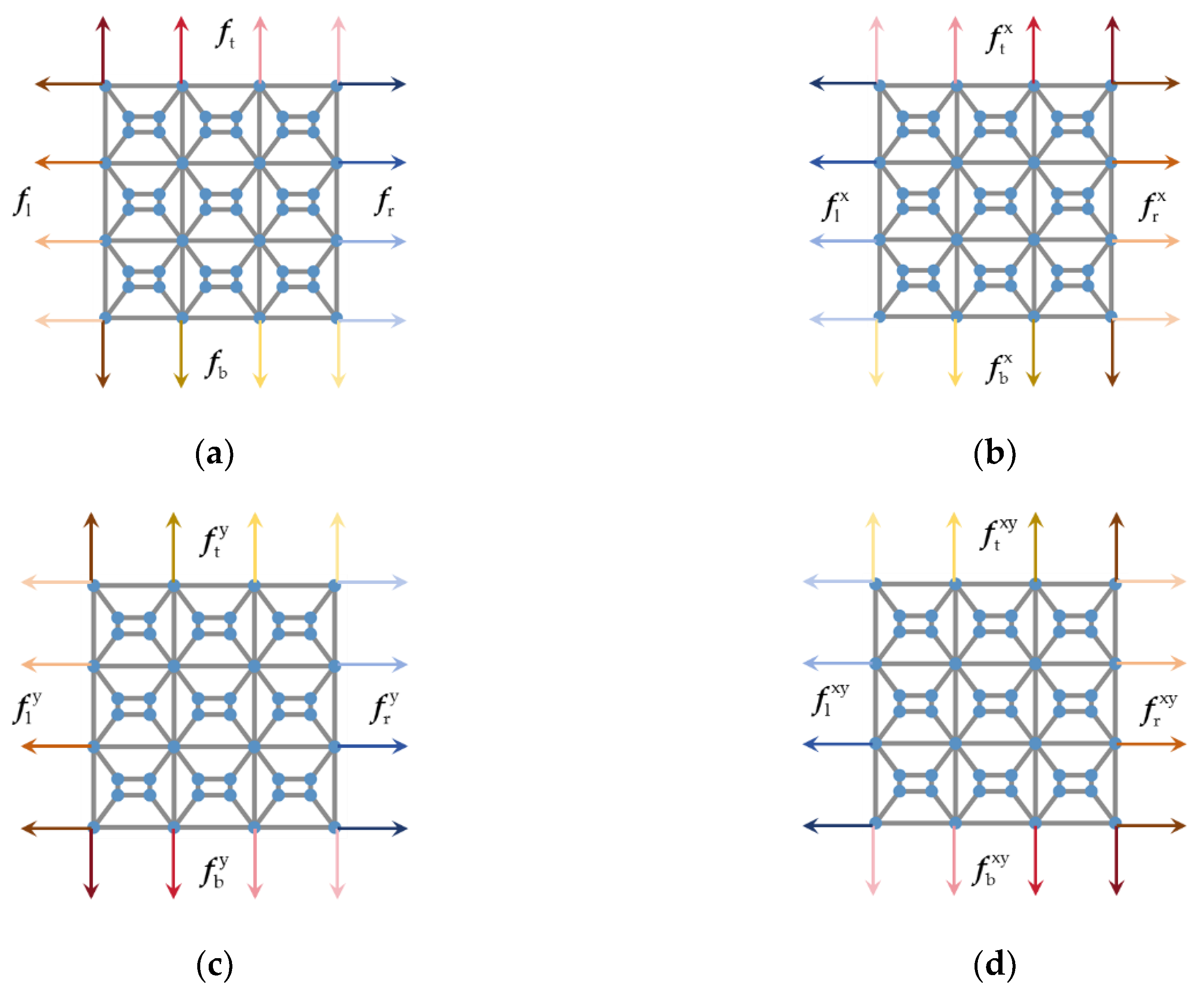
Figure 3.
Distributions of modal displacements on the boundaries of 3×3 metamaterials: (a) m; (b) mx; (c) my; (d) mxy;.
Figure 3.
Distributions of modal displacements on the boundaries of 3×3 metamaterials: (a) m; (b) mx; (c) my; (d) mxy;.
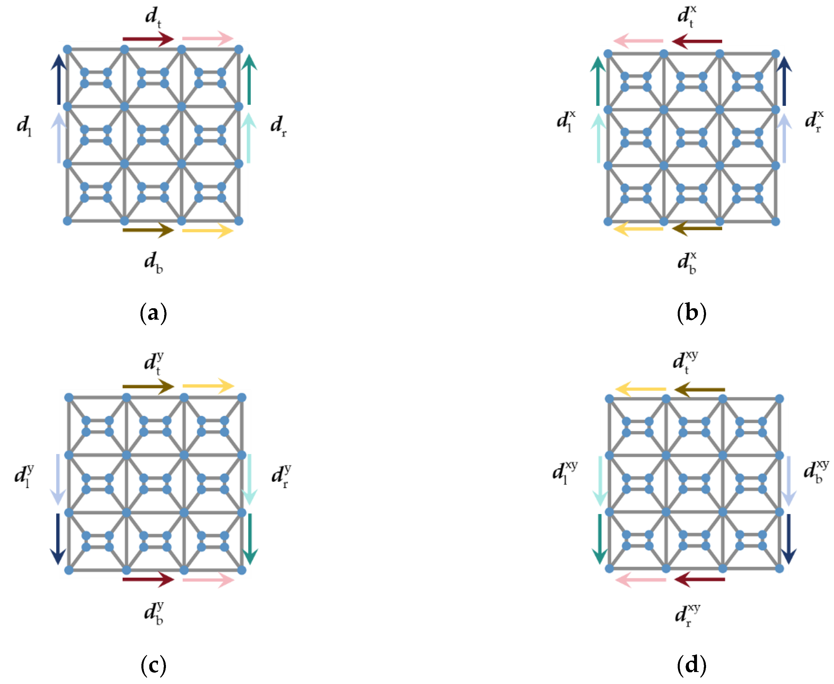
Figure 4.
Distributions of modal forces and displacements on the boundaries of M: (a) Forces; (b) Displacements.
Figure 4.
Distributions of modal forces and displacements on the boundaries of M: (a) Forces; (b) Displacements.
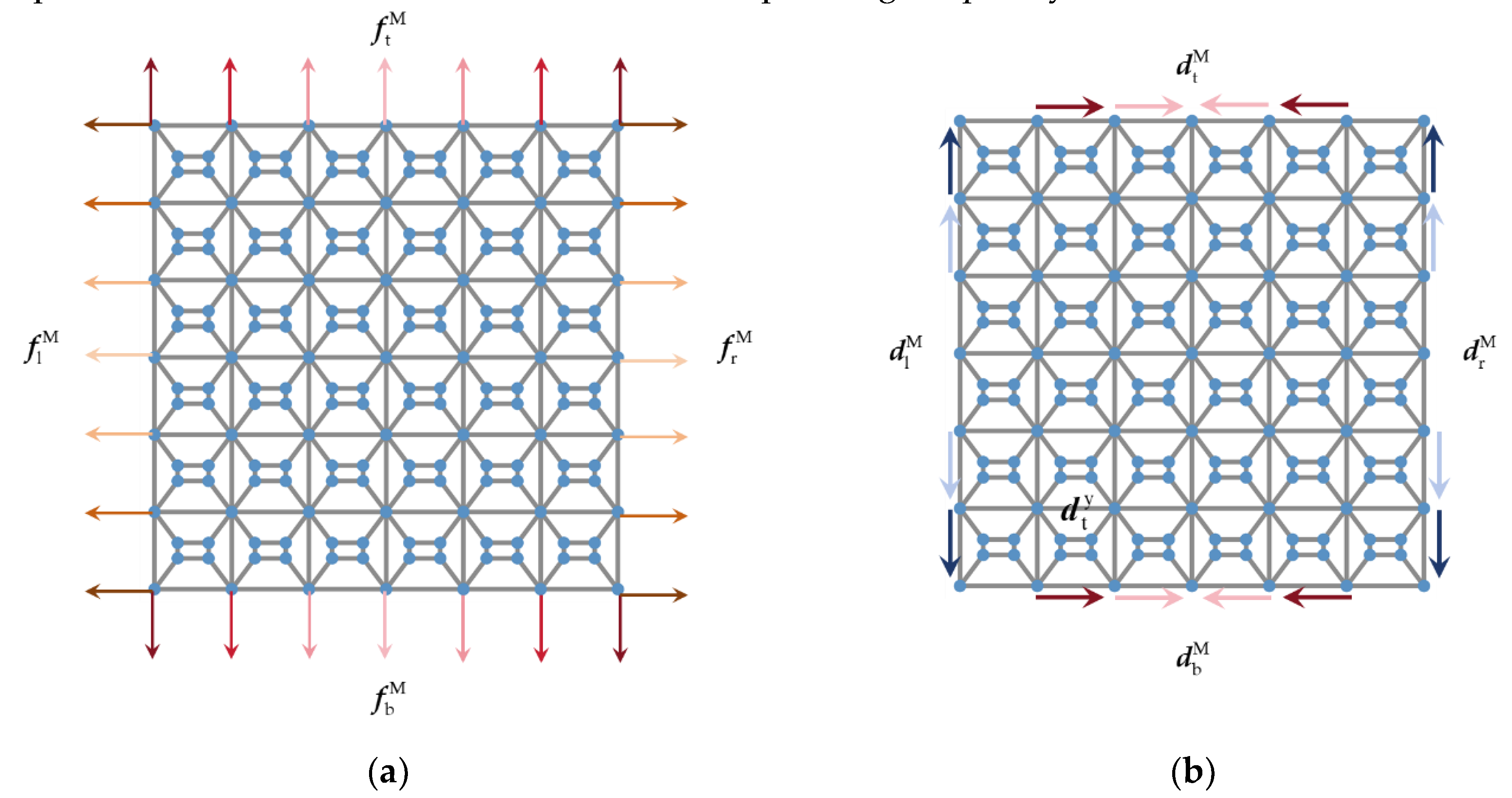
Figure 5.
An Illustrative bandgap.
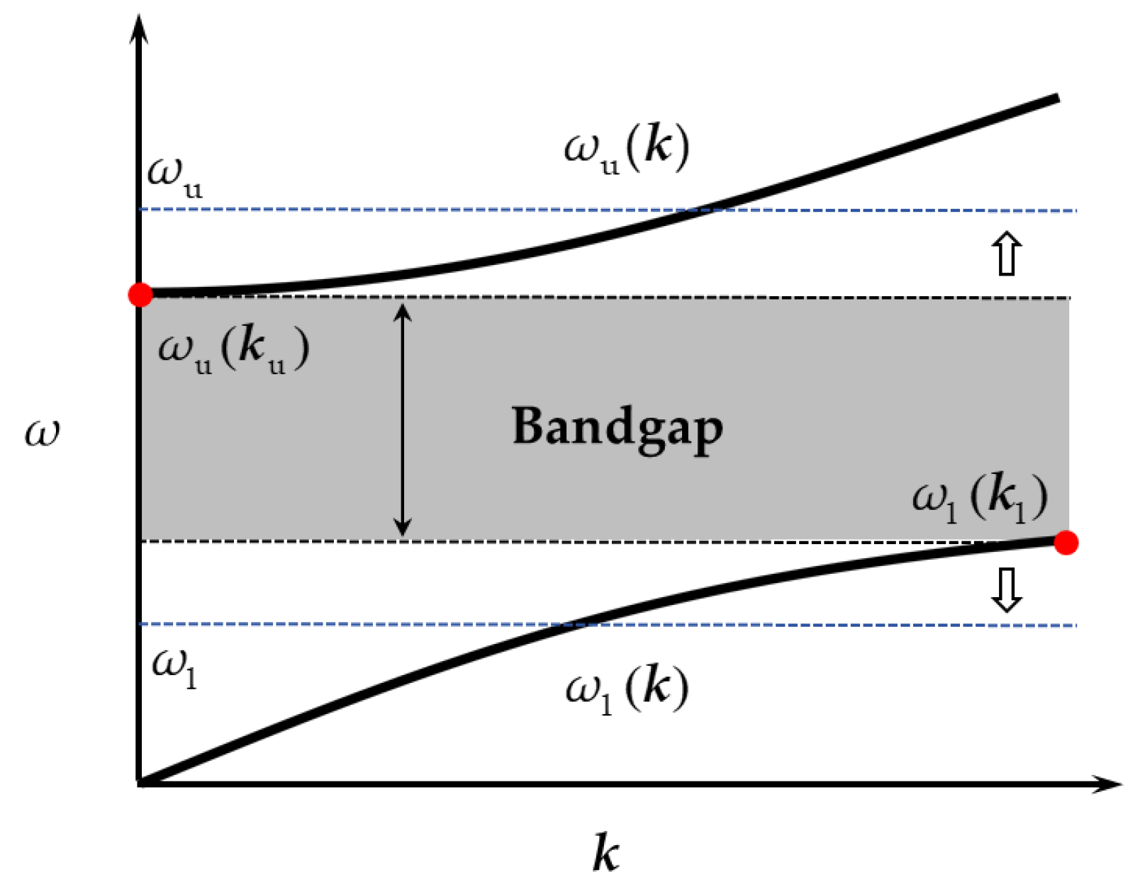
Figure 6.
A unit cell.
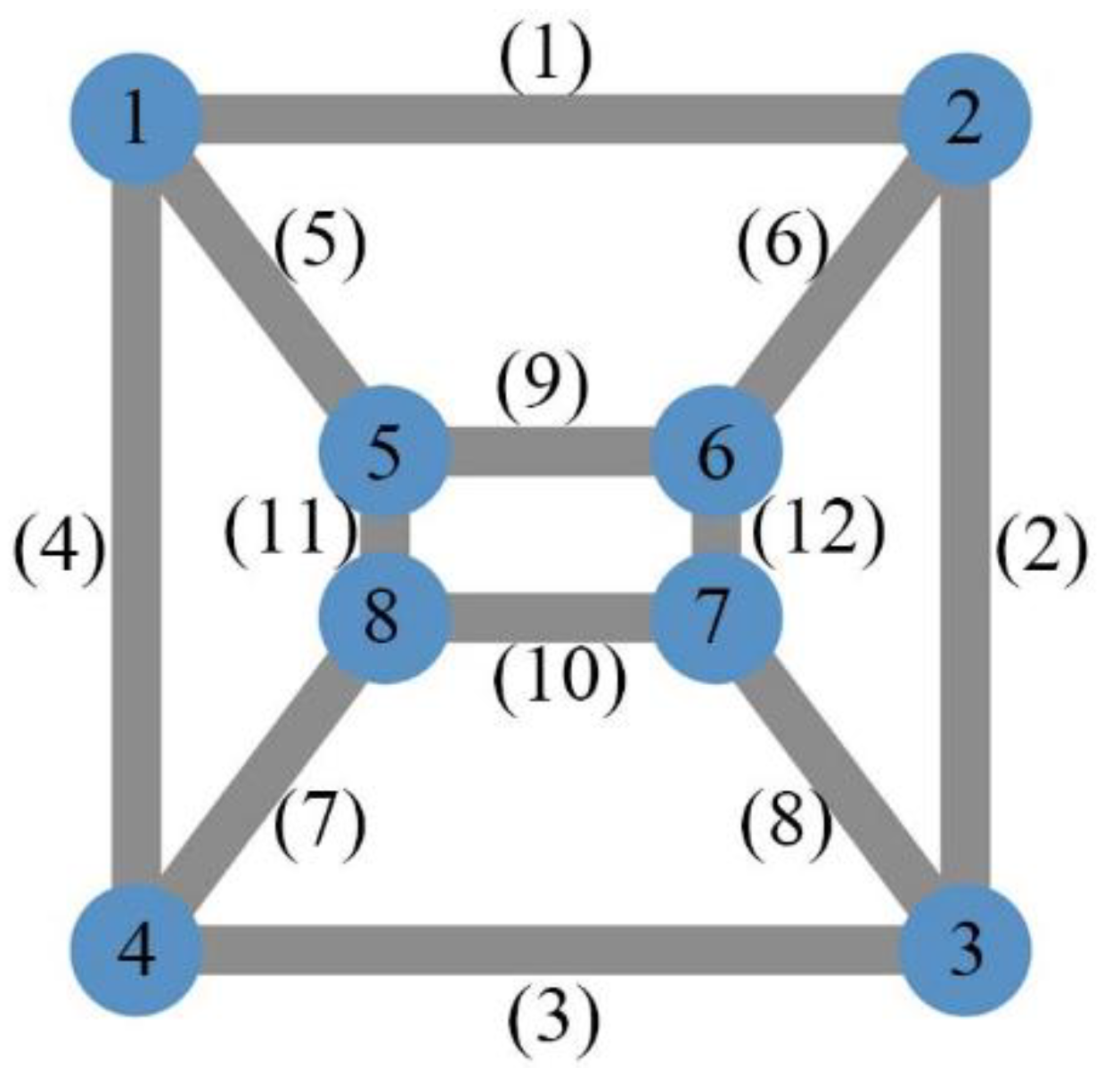
Figure 7.
Initial unit cell and corresponding frequency distribution of dispersion function: (a) Initial unit cell; (b) Frequency distribution of dispersion function.
Figure 7.
Initial unit cell and corresponding frequency distribution of dispersion function: (a) Initial unit cell; (b) Frequency distribution of dispersion function.
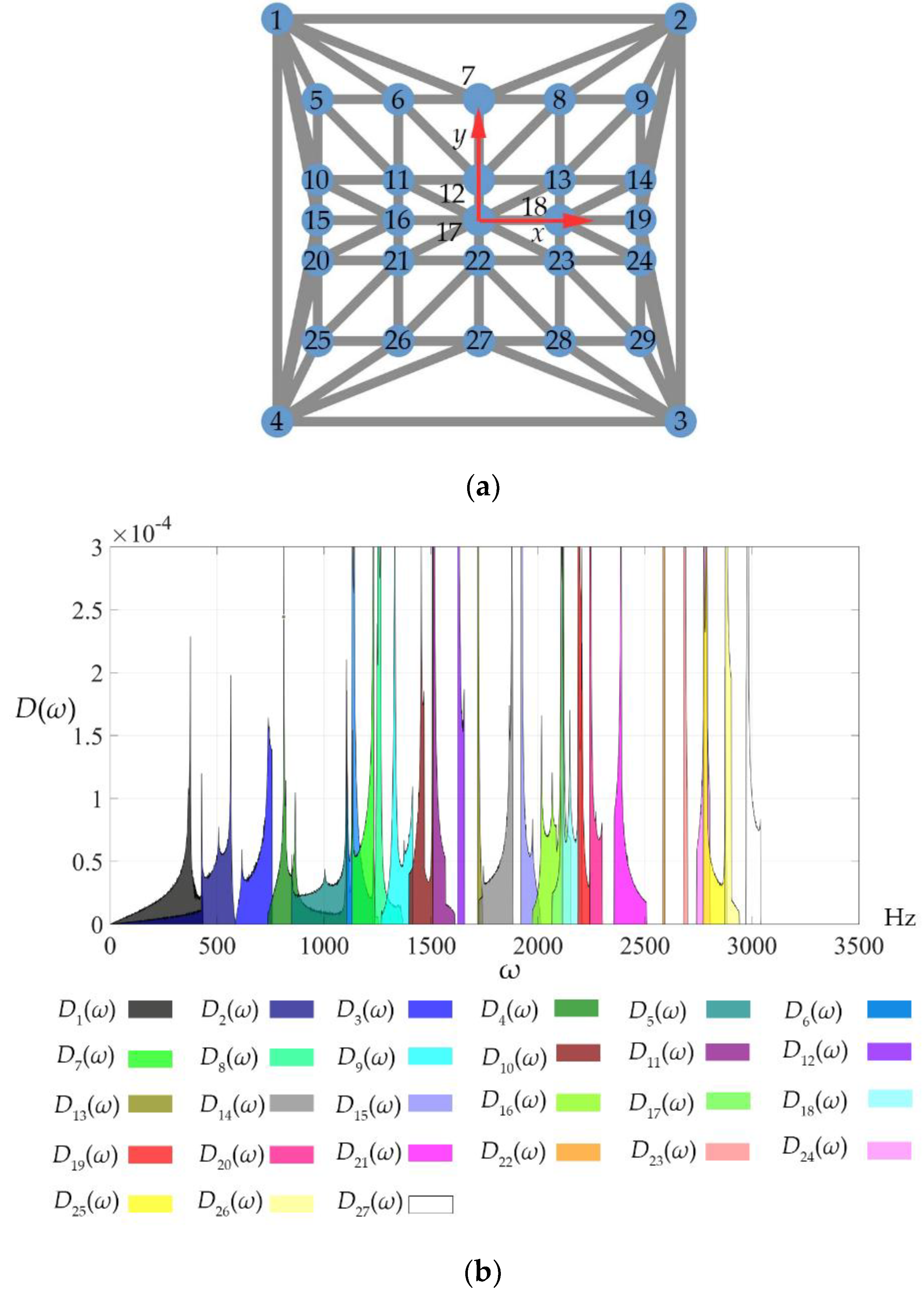
Figure 8.
Unit cell satisfying expected bandgap and corresponding frequency distribution of dispersion function: (a) Unit cell satisfying expected bandgap; (b) Frequency distribution of dispersion function.
Figure 8.
Unit cell satisfying expected bandgap and corresponding frequency distribution of dispersion function: (a) Unit cell satisfying expected bandgap; (b) Frequency distribution of dispersion function.
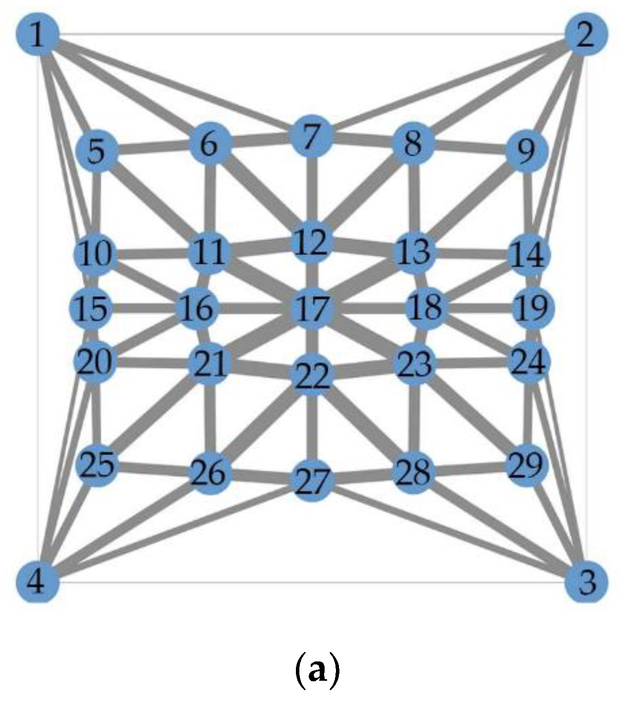
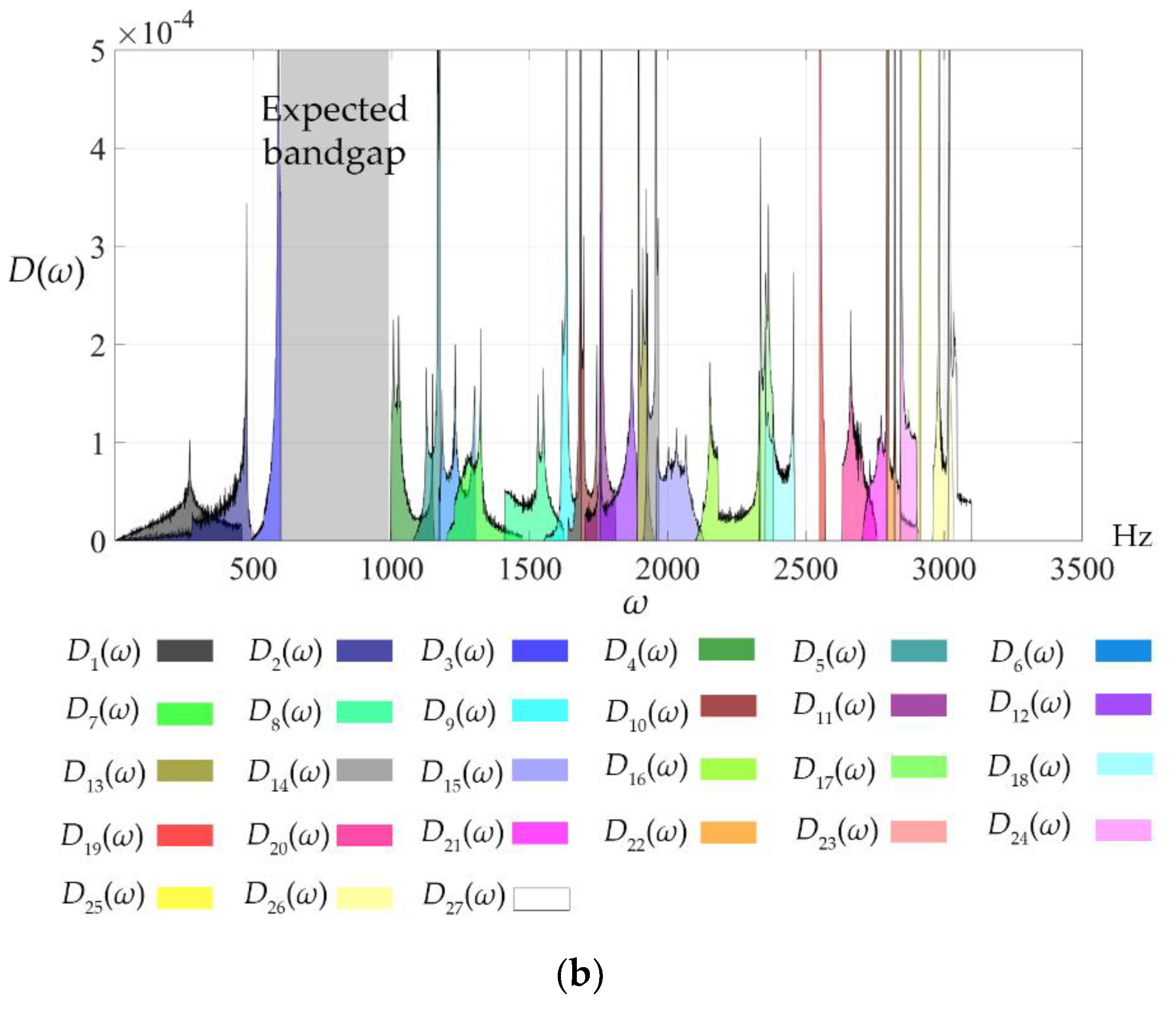
Figure 9.
Metamaterial consisting of designed unit cell and a boundary condition satisfying Table 1: (a) 4×4 metamaterial; (b) Boundary condition satisfying Table 1.
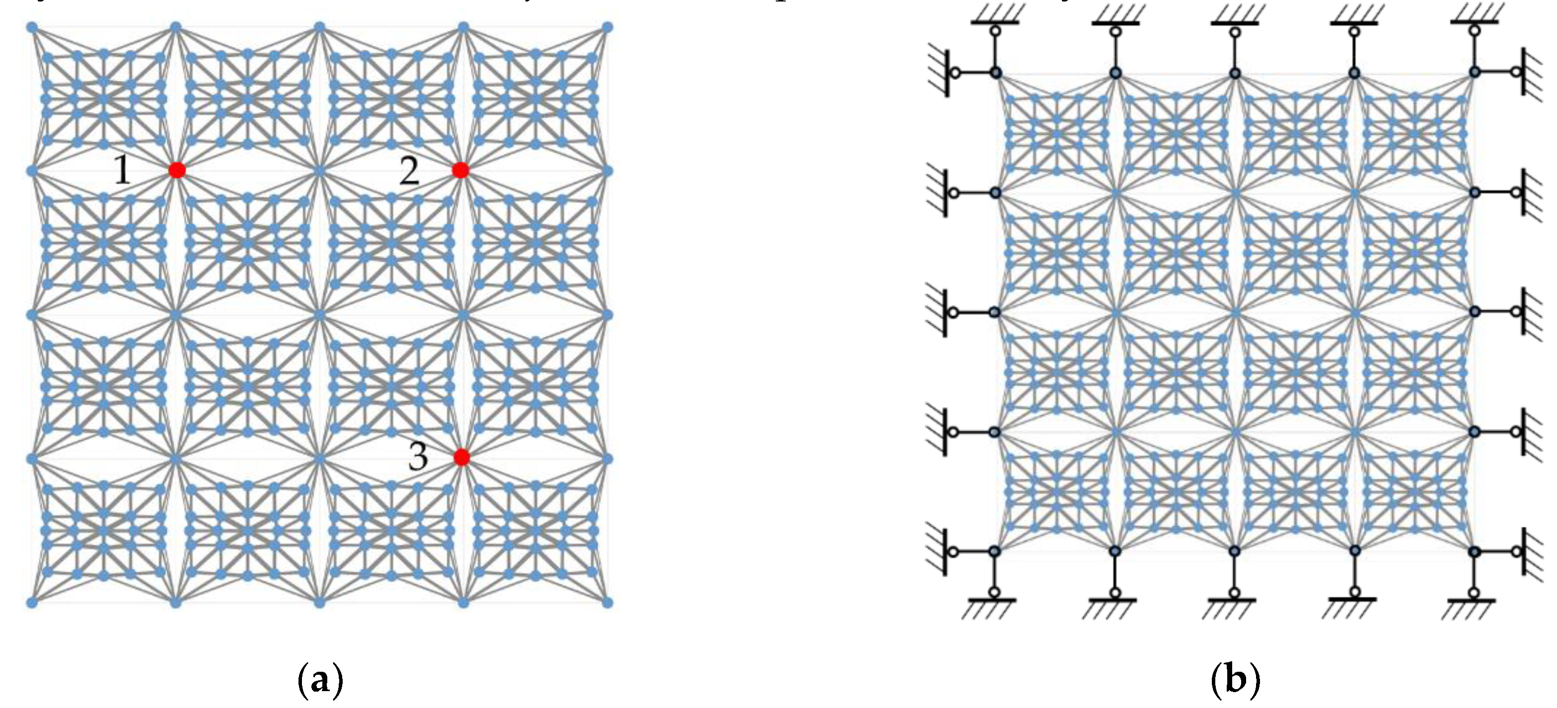
Figure 10.
Frequency-response curves and eigenfrequencies of PBC.
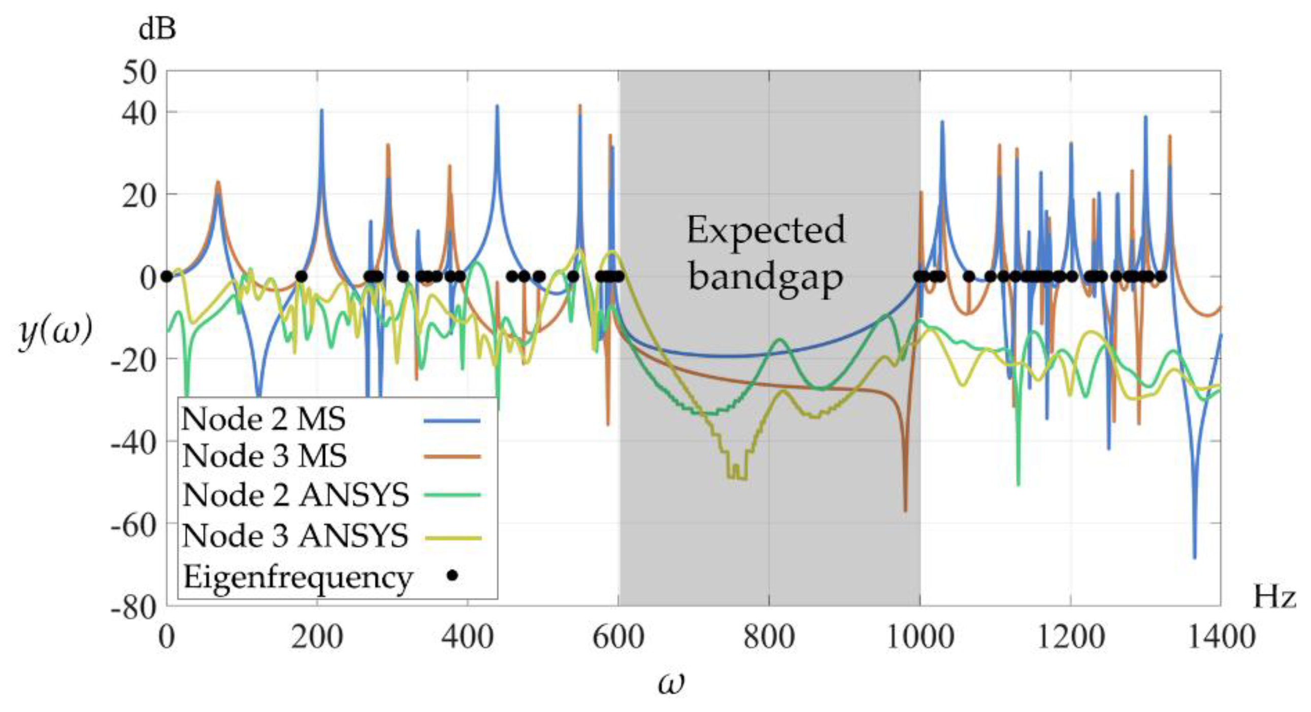
Figure 11.
Frequency-response curves and eigenfrequencies of FBC.
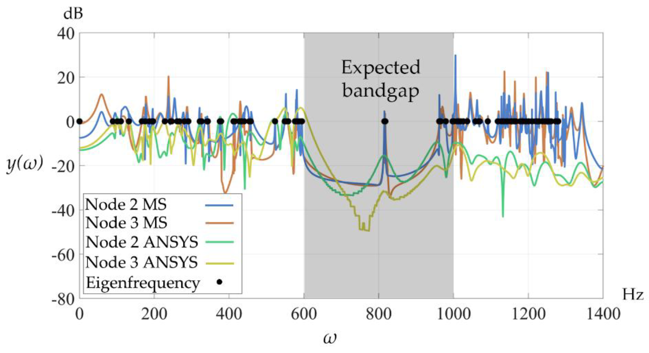
Figure 12.
Frequency-response curves and eigenfrequencies of SBC.
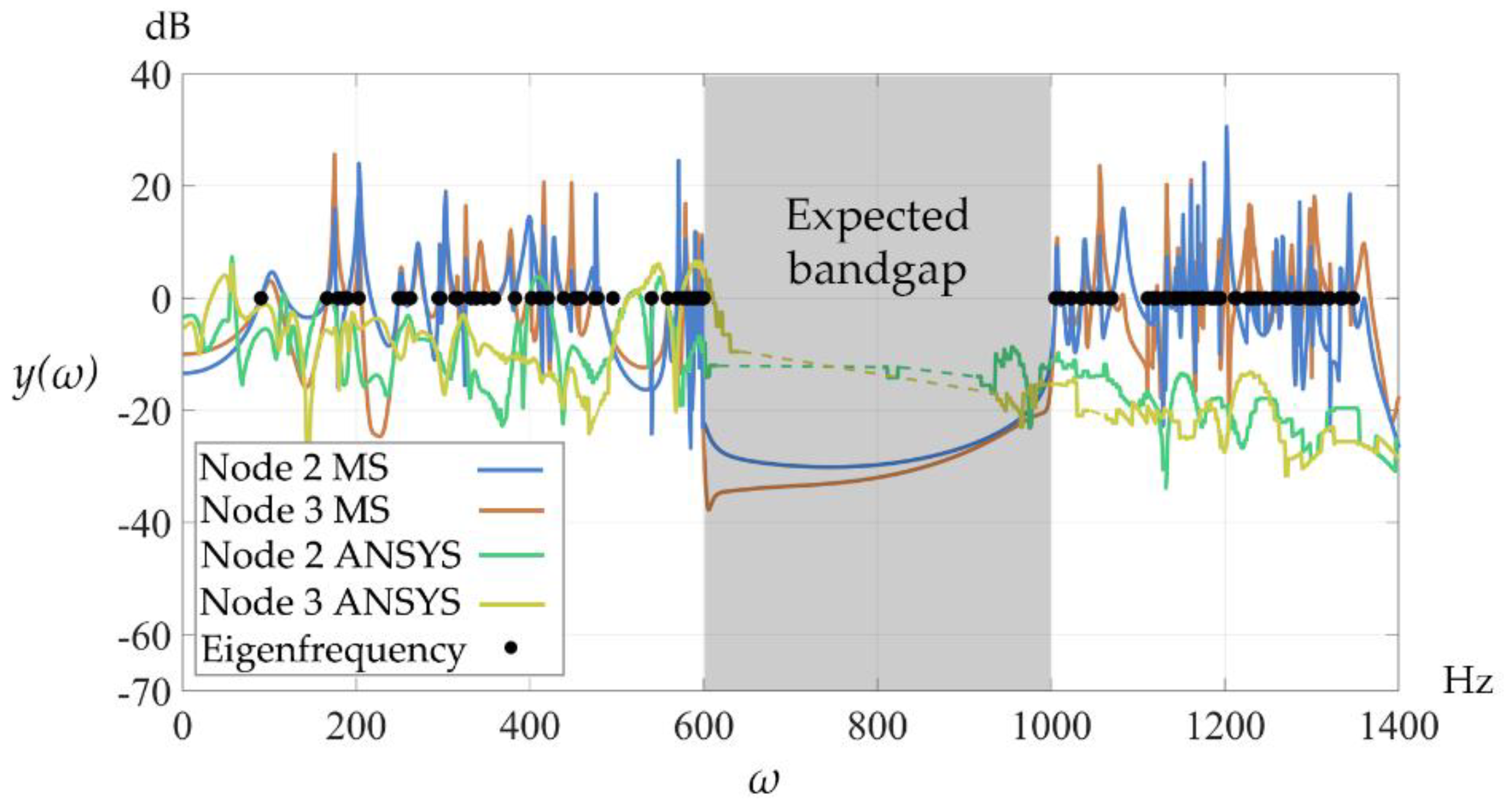
Figure 13.
Frequency-response curves and eigenfrequencies of SBCA.
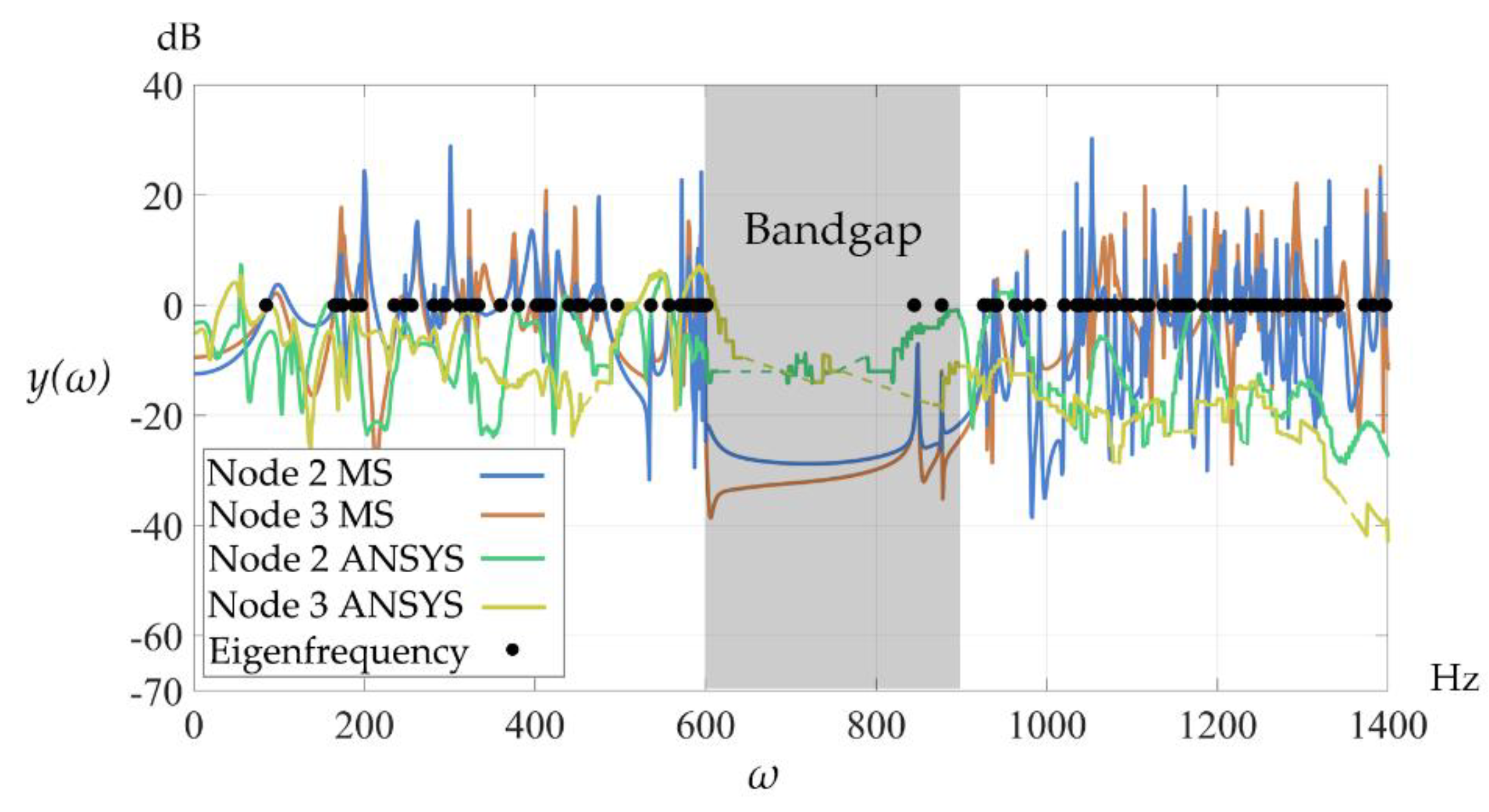

Table 1.
Boundary conditions of two-dimensional metamaterials for avoiding bandgap resonance.
| Case | Boundary condition | |
| x | y | |
| 1 | c1 | c1 |
| 2 | c2 | c1 |
| 3 | c1 | c2 |
| 4 | c2 | c2 |
Table 2.
Boundary conditions of three-dimensional metamaterials for avoiding bandgap resonance.
| Case | Boundary condition | ||
| x | y | z | |
| 1 | c2, c3 | c1, c3 | c1, c2 |
| 2 | c1 | c1, c3 | c1, c2 |
| 3 | c2, c3 | c2 | c1, c2 |
| 4 | c1 | c2 | c1, c2 |
| 5 | c2, c3 | c1, c3 | c3 |
| 6 | c1 | c1, c3 | c3 |
| 7 | c2, c3 | c2 | c3 |
| 8 | c1 | c2 | c3 |
Table 3.
Node coordinates of initial unit cell (mm).
| Node | Coordinate | Node | Coordinate | Node | Coordinate | |||
|---|---|---|---|---|---|---|---|---|
| x- | y- | x- | y- | x- | y- | |||
| 1 | -5.00 | 5.00 | 11 | -2.00 | 1.00 | 21 | -2.00 | -1.00 |
| 2 | 5.00 | 5.00 | 12 | -0.00 | 1.00 | 22 | 0.00 | -1.00 |
| 3 | 5.00 | -5.00 | 13 | 2.00 | 1.00 | 23 | 2.00 | -1.00 |
| 4 | -5.00 | -5.00 | 14 | 4.00 | 1.00 | 24 | 4.00 | -1.00 |
| 5 | -4.00 | 3.00 | 15 | -4.00 | 0.00 | 25 | -4.00 | -3.00 |
| 6 | -2.00 | 3.00 | 16 | -2.00 | 0.00 | 26 | -2.00 | -3.00 |
| 7 | 0.00 | 3.00 | 17 | 0.00 | 0.00 | 27 | 0.00 | -3.00 |
| 8 | 2.00 | 3.00 | 18 | 2.00 | 0.00 | 28 | 2.00 | -3.00 |
| 9 | 4.00 | 3.00 | 19 | 4.00 | 0.00 | 29 | 4.00 | -3.00 |
| 10 | -4.00 | 1.00 | 20 | -4.00 | -1.00 | |||
Table 4.
Element cross-sectional areas of the unit cell satisfying expected bandgap (mm2).
| Element | Area | Element | Area | Element | Area | Element | Area |
|---|---|---|---|---|---|---|---|
| 1-7 | 0.107 | 1-2 | 0.001 | 13-14 | 0.220 | 23-18 | 0.276 |
| 1-6 | 0.229 | 3-4 | 0.001 | 10-15 | 0.233 | 24-18 | 0.229 |
| 1-5 | 0.159 | 2-3 | 0.000 | 10-16 | 0.229 | 24-19 | 0.233 |
| 1-10 | 0.105 | 1-4 | 0.000 | 11-16 | 0.276 | 20-21 | 0.220 |
| 1-15 | 0.038 | 5-6 | 0.231 | 11-17 | 0.622 | 21-22 | 0.458 |
| 2-7 | 0.107 | 6-7 | 0.305 | 12-17 | 0.321 | 22-23 | 0.458 |
| 2-8 | 0.229 | 7-8 | 0.305 | 13-17 | 0.622 | 23-24 | 0.220 |
| 2-9 | 0.159 | 8-9 | 0.231 | 13-18 | 0.276 | 25-20 | 0.157 |
| 2-14 | 0.105 | 5-10 | 0.157 | 14-18 | 0.229 | 25-21 | 0.387 |
| 2-19 | 0.038 | 5-11 | 0.387 | 14-19 | 0.233 | 26-21 | 0.250 |
| 3-27 | 0.107 | 6-11 | 0.250 | 15-16 | 0.202 | 26-22 | 0.509 |
| 3-28 | 0.229 | 6-12 | 0.509 | 16-17 | 0.261 | 27-22 | 0.246 |
| 3-29 | 0.159 | 7-12 | 0.246 | 17-18 | 0.261 | 28-22 | 0.509 |
| 3-24 | 0.105 | 8-12 | 0.509 | 18-19 | 0.202 | 28-23 | 0.250 |
| 3-19 | 0.038 | 8-13 | 0.250 | 20-15 | 0.233 | 29-23 | 0.387 |
| 4-27 | 0.107 | 9-13 | 0.387 | 20-16 | 0.229 | 29-24 | 0.157 |
| 4-26 | 0.229 | 9-14 | 0.157 | 21-16 | 0.276 | 25-26 | 0.231 |
| 4-25 | 0.159 | 10-11 | 0.220 | 21-17 | 0.622 | 26-27 | 0.305 |
| 4-20 | 0.105 | 11-12 | 0.458 | 22-17 | 0.321 | 27-28 | 0.305 |
| 4-15 | 0.038 | 12-13 | 0.458 | 23-17 | 0.622 | 28-29 | 0.231 |
Table 5.
Node coordinates of the unit cell satisfying expected bandgap (mm).
| Node | Coordinate | Node | Coordinate | Node | Coordinate | |||
|---|---|---|---|---|---|---|---|---|
| x- | y- | x- | y- | x- | y- | |||
| 1 | -5.00 | 5.00 | 11 | -1.87 | 1.01 | 21 | -1.87 | -1.01 |
| 2 | 5.00 | 5.00 | 12 | 0.00 | 1.21 | 22 | 0.00 | -1.21 |
| 3 | 5.00 | -5.00 | 13 | 1.87 | 1.01 | 23 | 1.87 | -1.01 |
| 4 | -5.00 | -5.00 | 14 | 3.95 | 0.98 | 24 | 3.95 | -0.98 |
| 5 | -3.92 | 2.87 | 15 | -4.03 | 0.00 | 25 | -3.92 | -2.87 |
| 6 | -1.85 | 3.01 | 16 | -2.09 | 0.00 | 26 | -1.85 | -3.01 |
| 7 | 0.00 | 3.14 | 17 | 0.00 | 0.00 | 27 | 0.00 | -3.14 |
| 8 | 1.85 | 3.01 | 18 | 2.09 | 0.00 | 28 | 1.85 | -2.99 |
| 9 | 3.92 | 2.87 | 19 | 4.03 | 0.00 | 29 | 3.92 | -2.87 |
| 10 | -3.95 | 0.98 | 20 | -3.95 | -0.98 | |||
Disclaimer/Publisher’s Note: The statements, opinions and data contained in all publications are solely those of the individual author(s) and contributor(s) and not of MDPI and/or the editor(s). MDPI and/or the editor(s) disclaim responsibility for any injury to people or property resulting from any ideas, methods, instructions or products referred to in the content. |
© 2025 by the authors. Licensee MDPI, Basel, Switzerland. This article is an open access article distributed under the terms and conditions of the Creative Commons Attribution (CC BY) license (http://creativecommons.org/licenses/by/4.0/).
Copyright: This open access article is published under a Creative Commons CC BY 4.0 license, which permit the free download, distribution, and reuse, provided that the author and preprint are cited in any reuse.


