Submitted:
24 July 2025
Posted:
25 July 2025
Read the latest preprint version here
Abstract
Previous studies have shown that hazard ratios between treatment groups estimated with the Cox model are uninterpretable because the indefinite baseline hazard of the model fails to identify temporal change in the risk set composition due to treatment assignment and unobserved factors among multiple, contradictory scenarios. To alleviate this problem, especially in studies based on observational data with uncontrolled dynamic treatment and real-time measurement of many covariates, we propose abandoning the baseline hazard and using machine learning to explicitly model the change in the risk set with or without latent variables. For this framework, we clarify the context in which hazard ratios can be causally interpreted, and then develop a method based on Neyman orthogonality to compute debiased maximum-likelihood estimators of hazard ratios. Computing the constructed estimators is more efficient than computing those based on weighted regression with marginal structural Cox models. Numerical simulations confirm that the proposed method identifies the ground truth with minimal bias. These results lay the foundation for developing a useful, alternative method for causal inference with uncontrolled, observational data in modern epidemiology.
Keywords:
survival analysis
; hazard ratio
; machine learning
; causal inference
; kernel method
1. Introduction
The use of hazard ratios to measure the causal effect of treatment has recently come under debate. Although it has been standard practice in epidemiological studies to examine hazard ratios using the Cox proportional model and its modified versions [1,2], several studies [3,4,5] have noted that hazard ratios are uninterpretable with regard to causation (see Martinussen (2022) [6] for a review). In particular, Martinussen et al. (2020) [5] provided concrete examples of data-generating processes in which the Cox model is correctly specified, but estimated hazard ratios are difficult to interpret. The main difficulty is that time courses of different study populations with different treatment effects are described by the same Cox model with the same set of parameter values. Although a few authors have rebutted the uninterpretability of hazard ratios in the Cox model [7,8,9], the issue concerning the unidentifiability with multiple, contradictory scenarios as posed by Martinussen et al. (2020) [5] remains unresolved.
To address this issue, researchers have sought alternative measures of causal treatment effect, such as differences between counterfactual survival functions or restricted mean survival time [10,11,12]. Methods for applying machine learning to estimate these measures have also been developed [13,14,15]. However, these measures are only applicable to simple, well-controlled settings, such as randomized clinical trials or observational studies of several covariate-adjusted groups with different baseline treatments, despite such studies making few assumptions about data-generating processes in other respects, as suggested by semiparametric theories for causal inference (see, e.g., Ref.[16]). Modern epidemiology increasingly requires methods for analyzing large quantities of observational data acquired in a more uncontrolled, dynamic manner, in which many covariates are measured in real-time. Examples of such data are electronic medical or health records and data acquired by electronic devices for health promotion [17]. The marginal structural Cox model potentially used for this purpose [18] suffers from the uninterpretability problem described above, and thus, development of an alternative method is required.
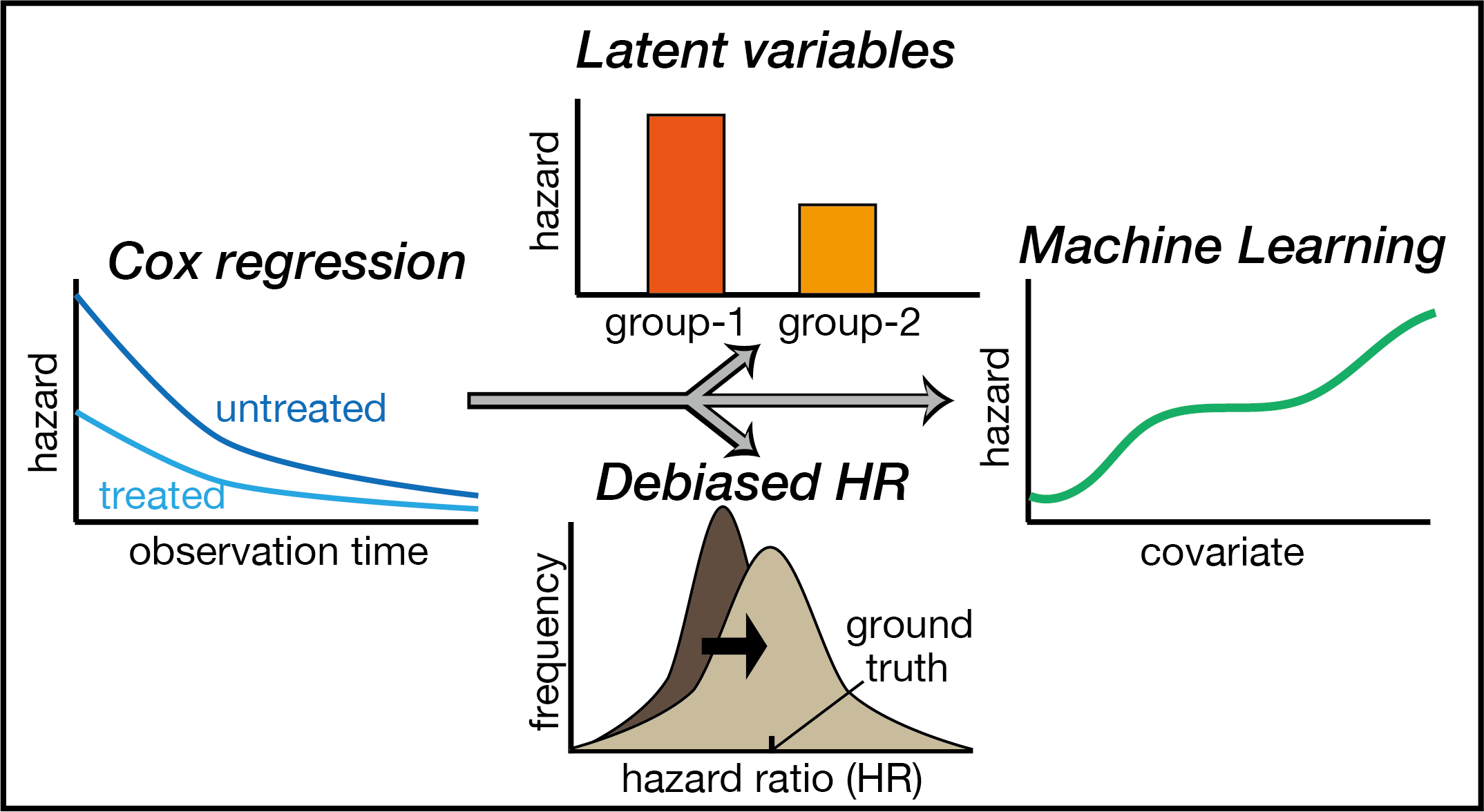
The present study proposes a strategy to model heterogeneous risk groups in a study population by using an exponential hazard model based on time-dependent treatment variables and covariates, but with no indefinite baseline hazard. Although Martinussen et al. (2020) did not explicitly describe the role of the baseline hazard in the problem about interpretability, it was the indefinite baseline hazard that allows the Cox model to be correctly specified for arbitrary temporal change in the risk set, namely, what they call “selection”. Thus, we abandon the semiparametric nature of the Cox models, and instead exploit the descriptive power of machine learning to capture how the risk set changes over time. This approach can now be implemented due to recent advances in incorporating machine learning into rigorous statistical analysis with effect estimation [19,20]. Prior to this development, machine learning could be used for only outcome prediction in epidemiology, because estimation with machine learning was biased. We thus develop an algorithm that debiases maximum-likelihood (ML) estimators of hazard ratios in the model, using the framework of doubly robust, debiased machine learning (DML) based on Neyman orthogonality (see Ref.[21] for an introductory review). Under mostly testable assumptions, the estimated hazard ratios can be interpreted as a measure of causal treatment effect. We show that this approach can be systematically extended to settings with latent variables. In simulation studies with clinically plausible settings, the results confirm that the proposed method identifies the ground truth with minimal bias. In these results, we also show that the proposed ML approach has multiple advantages over Cox’s maximum-partial-likelihood (MPL) approach.
2. Theories and Methods
2.1. Exponential Parametric Hazard Model Combined with Machine Learning
We consider observational studies in which the occurrence or absence of an event of interest in subjects randomly sampled from a large population and indexed by is longitudinally observed over time (indexed by t) during a noninformatively right-censored period, . With a set of time-dependent covariates, collectively denoted by , we strive to identify the effect of time-dependent treatment described by a collection of binary variables ). For clarity of presentation, we assume that at most a single treatment variable can take a value of unity, and the remaining variables must be zero. Consider an exponential hazard model whose conditional hazard is given by
where is a set of parameters corresponding to the natural logarithm of the hazard ratio of the untreated samples to samples treated to different extents, and the function f describes the risk variation due to the given set of covariates, which we adjust using a machine learning model (i.e., a set of functions in which f lies). In addition, hereinafter, denotes the transposition of vectors and matrices. Note that the above model lacks the baseline hazard as a function of t (the time elapsed after enrollment). The covariate can include temporal information, such as date and durations of suffered disorders, but not t itself.
Suppose that a subset of subjects (indexed by i) experiences an event of interest at time in the observation period, and the other subjects experience no such event. The full log-likelihood for this observation is then given by
(see, e.g., Ref.[22]), where is the indicator function that returns unity for and zero otherwise. To see the meaning of Eq.(2), we consider how the hazard model describes the occurrence of an event in a small interval . Assuming for the moment that (i) is continuous with respect to s and (ii) over , the likelihoods of occurrence and non-occurrence of an event in this period conditioned on event-free survival at time t are and , respectively, up to the first order in . Simple computations show that the log-likelihood for this binary observation is
2.2. Causal Inference and ML Estimation
This section clarifies the causal interpretation of the estimation results in the model described in the previous section and discusses the necessary assumptions that support this interpretation. First, we make the conventional assumptions of consistency, no unmeasured confounder (ignorability), and positivity.
Assumption 1 (consistency).
For any counterfactual treatment schedule a, we have, and .
Assumption 2 (no unmeasured confounder):
For some , we have, for any t and any counterfactual treatment schedule a,
Assumption 3 (positivity):
For any and any , we have .
Here, the set subscript, such as , denotes the collection of all variables with subscripts included in the set. Throughout the paper, P denotes the ground-truth (conditional) probability of the argument variables. We have used variables for for a technical reason that and must be determined on the basis of the past information. This may be replaced by some finite interval before the enrollment at for which the information about treatment and covariate is available.
Next, in addition to the above, we make the following assumption about the regularity of hazard.
Assumption 4 (regularity of hazard):
holds almost surely.
Remark 1:
Assumption 2 essentially implies that the treatment at time t does not affect the time evolution of covariate X for a subsequent period as seen through the following argument. First, we have
holds, where the first and second equalities are due to no unmeasured confounder and consistency, respectively. If the time evolution of covariates is immediately affected by the treatment schedule, and if outcome is immediately affected by the covariates, then under the conditioning on , depends on the value of A, and hence, depends on A, which contradicts the assumption. A similar assumption is conventionally made in the analysis of observational data with a marginal structural Cox model [18].
In addition to Assumptions 1–4, we assume that the model in Eq.(1) is correctly specified. More precisely, we make the following four assumptions:
Assumption 5 (hazard conditionally independent of past treatment and covariate).
For any , , and , we almost surely have,
Assumption 6 (homogeneous treatment effect).
For any and any , the hazard contrast,
takes a constant value regardless of the value of x.
Assumption 7 (time-homogeneous hazard):
The hazard is independent of its timing during the observation period. Mathematically, for any , and any fixed and ,
Assumption 8 (correctly specified machine-learning model):
There exist unique and that satisfy
where is the set of Borel-measurable functions.
Remark 2:
Assumptions 5–7 can be validated by extending the model to incorporate the effect of past treatment and covariates, inhomogeneous treatment effect, and time inhomogeneity, respectively. The original and extended models can then be compared in terms of, for example, Bayesian model evidence (BME) (see, e.g., Chapter 3 of Ref.[23]). If Assumption 5 is violated, the definition of the treatment variables and covariates may be extended so that the current value retains past information. This is the same strategy as employed for designing variables in a marginal structural Cox model [18]. If Assumption 6 is violated, the model may be extended by incorporating covariate-dependent heterogeneous treatment effect. Violation of Assumption 7 indicates that variations in covariate values do not account for the temporal change in the risk set. In this case, additional covariates or extending the model with latent variables (as described below) may be considered. Finally, Assumption 8 is an a priori assumption that stems from the fact in statistical learning that inference in the function space requires a regularity assumption.
Proposition 1.
Let the maximizer of the expected likelihood be
Under Assumptions 1–8, suppose two possible treatment schedules such that holds, and that and (or ) holds for for some . Then, we have, for any sample path for covariate,
Proof.
We have,
The first and second equalities are due to no unmeasured confounder and consistency (Assumptions 2 and 1), respectively. The last equality is due to Assumptions 4 and 5. Identifying the last line with the ML estimator is straightforward as follows. Using Assumptions 4 and 5 and Eq.(3), the expected likelihood is represented as
Here, terms independent of and f have been regarded as constants, and the integration with respect to the ground-truth probability measure has been denoted by . Differentiating this representation gives
With Assumptions 6 and 7, it is seen that these derivatives vanish if and only if
hold almost everywhere in with respect to , and the concavity of the expected log-likelihood ensures that this solution is the maximizer. □
Remark 3-1.
Suppose that Assumption 2 holds for arbitrary . Then, for arbitrary , we obtain
with the aid of Assumptions 1–5 in the same manner as we have done for Eqs.(6) and (13). If we can assume with probability one at some , the above equation implies that the counterfactual survival function is given by
Although measures of causal effects can be calculated from this relation, doing so requires an unbiased estimation of , which is possible, only if a simple model can be used to estimate f without modeling error.
Remark 3-2.
The quantity in Eq.(12) is a covariate-adjusted hazard contrast for two counterfactual treatments that branch at time t, so it can be interpreted as a measure of causal effect. In the setting discussed in Ref.[18], this corresponds to the treatment effect measured in the next month (for which covariates at each month can be regarded as baseline covariates [24]).
Remark 3-3.
As discussed in Martinussen et al. (2022) [6], of more interest is the quantity
for two arbitrary counterfactual treatment schedules that branch before t. A stronger untestable assumption is required for this to be related to the hazard ratios. For example,
for any t and any counterfactual treatment schedules . This condition is satisfied if no unmeasured factors affect the outcome, as described by the causal graph in Figure 1(A). If unmeasured factors affect the outcome, as described by the causal graph in Figure 1(B), the above conditions are not satisfied. Although the assumption of time-homogeneity (Assumption 7) is strong and does not allow temporal change in the heterogeneity of risk to be left unmodeled, it does not completely exclude the existence of unmeasured factors affecting outcome. For example, suppose that the survival of subjects for an arbitrary counterfactual treatment schedule a is described by
where is the so called “shot noise” described by Dirac delta functions centered at time points determined by a homogeneous Poisson point process . The subject-wise random effect of shared between and then violates Eq.(21), whereas at different time points are independent and do not influence the time-homogeneity.
2.3. Debiasing ML Estimators
Next, we assume that we have consistent estimators for and f that are the maximizers of the empirical log-likelihood in Eq.(2) in the presence of a suitable regularizer. Although a large body of the machine-learning literature presents such consistent estimators, they are biased in the sense that we cannot expect for the number of subjects . This situation prohibits making a decision on the significance of estimated results. However, we can apply to this problem debiased machine learning based on Neyman orthogonality and developed by Chernozhukov et al. (2018) [20]. Chernozhukov et al. (2018) describe how to systematically debias ML estimators and other M-estimators. Applying their idea to our problem setting yields debiased estimators of .
Definition 1 (Neyman orthogonal scores).Suppose that an estimator of quantities of interest is given as a zero of the empirical average of score functions for i.i.d. data :
where the third argument in the summands is a (possibly infinite-dimensional) nuisance parameter and an estimator of an optimal value is used. Then, ϕ is said to be “Neyman orthogonal,” if it satisfies
where, in the second line, denotes the Gateaux derivative operator [25].
Given a few conditions on the regularity of score functions and the convergence of nuisance parameters, Chernozhukov et al. [20] proved . In the following, we construct such orthogonal scores from the log-likelihood in Eq.(2).
Proposition 2 (Neyman orthogonal scores derived from log-likelihood).
Assume that the positive Borel measures () defined as
() are absolutely continuous to each other and have Radon-Nykodym derivatives
for which denotes such that , and is a measurable function on . Then, the score functions for estimating θ,
, are Neyman orthogonal. Here, D denotes .
Proof.
Consider the following hazard model that includes the heterogeneous treatment effect:
Because we assumed the homogeneity of the treatment effect (Assumption 6), we have, for arbitrary ,
Let the first line on the right-hand side of Eq.(28) be and the second line be . Note that with and coincides with the above equation with . Similarly, for arbitrary , we have
Subtracting the sum of Eq.(30) for all k from Eq.(31) for , we obtain . Hence, has been proven.
Next, we examine the Gateaux derivatives of the expected scores with respect to the nuisance parameters . First, the derivative of with respect to at and is
The combination of Eqs.(30) and (31) again proves the last equality. The derivative with respect to f at , and is given by
Eq.(27) shows that the expected values of the two integrands in the second line cancel out, which proves the last equality. □
Remark 4-1.
In the above proof, Assumption 8 assures that the argument of the Gateaux derivative does not need to belong to . As one might notice, the crux of the construction lies in balancing the second and third terms of Eq.(28) by . Roughly speaking, for each value of covariates, weights the integrand with the inverse-treatment-probability for and . Here, note that this treatment probability is marginalized with respect to time.
Remark 4-2.
Chernozhukov et al. (2018) [20] present a systematic method to derive orthogonal scores from likelihood [see Eq.(2.29) of Ref.[20]. The straightforward application of their method results in more complex scores, each of which contains all of . As we see in this fact, multiple methods for orthogonalization are available. Prioritizing the simple explanation, we propose using the above.
2.4. Estimation Algorithm
- In this section, we describe a concrete procedure for computing the debiased estimators for the hazard ratios for treatment.
- Step 1: Estimation of f and .
- Plug-in estimators for f and are used to debias the estimation of , following a procedure called “cross-fitting”. To debias , the estimation errors in f and must be independent of the data in the argument of score functions. Thus, the entire dataset D are first partitioned into M groups of approximately equal size (. Using , and , is estimated as the maximizer of the log-likelihood of with a suitable regularizer. Similarly, is estimated as a regularized solution for the following logistic regression:To determine the regularization parameters for estimating f, we use BME averaged over the M folds. Because the logarithmic loss in Eq.(34) may underestimate the error due to large and in the score functions, we suggest computing the following cross-validation error in Eq.(33) which is targeting:The above error design exploits the fact that, for ,Here, the trivial solution also minimizes and should be avoided by checking BME as well.
- Step 2: Validation of hypotheses. The assumptions for Proposition 1 should be validated. Validating Assumptions 5–7 can be done by carrying out the ML estimation with replacement of by , by , by and by , respectively, and comparing the resultant BME (i.e., the posterior probabilities of the null and alternative hypotheses).
- Step 3: Debiased estimation of and its standard error.
- The estimator of is obtained as the zero of the following:The asymptotic standard error of the estimator is given by withThus, in the simulation study described below, the square roots of the diagonal elements of serve to scale the errors from the ground truth to obtain the t-statistics.
2.5. Extension to Models with Latent Variables
Suppose that the Assumption 7 is violated due to the presence of unobserved factors affecting the outcome, and covariates cannot adjust the resultant temporal change in the risk set. In this case, as we see in the simulation study below, the inclusion of the time elapsed after enrollment in the set of covariates may improve the description of event occurrence in terms of BME. For such cases, if additional data about the unobserved factors cannot be acquired, the only alternative is to explicitly model the unobserved factors as latent variables.
To simplify the argument and notation, let us assume that the unobserved factor (denoted by ) is a single time-independent binary variable (e.g., a variable indicating the presence or absence of a genetic risk factor). Suppose that we attempt to explicitly model W with a latent variable and define the distribution of Z and its influence on the outcome as and with parameters and , respectively. For example, in the simulation study described below, we use a logistic model that determines the distribution of the latent variable based on baseline covariate values:
and we extend the hazard model as
The same argument for Proposition 1 applies to this model. Suppose that the ground truth is described by
and
regardless of the values of x, a and t. Then, replacing X with the combination or in Assumptions 1–8 and assuming that the model is identifiable, one obtains the same result as in Proposition 1.
Then, one can also derive Neyman-orthogonal scores for this model as well. The logarithm of marginal likelihood of outcome is given by
with the aid of variational distributions . Hereafter, we use the variable without time subscripts, such as , which denotes the collection of variables throughout the observation period and can be understood from the context. Although optimal values for depend on and f, variable can also be regarded as an independent nuisance parameter. Naive non-orthogonal scores for ML estimation are obtained by simply differentiating the marginal likelihood with respect to as
These score functions can be orthogonalized in the same manner as for the model without latent variables.
Proposition 3 (Neyman orthogonal scores with a binary latent variable)
Assume that the positive Borel measures () defined as
() are absolutely continuous to each other with Radon-Nykodym derivatives
for which denotes such that , and is a measurable function on . Here, we have used random variable
Then, score functions for estimating
are Neyman orthogonal scores that can be used to debias the maximizer of the marginal log-likelihood in Eq.(44).
Proof.
The outline of the proof is the same as that for Proposition 2, and so is omitted here. □
2.6. Inference with Multiple-Kernel Models
In the simulation study described below, we use multiple-kernel models for the estimation of f and [26]. Statistical properties of estimation with multiple-kernel models under a 1-norm, 2-norm or mixed-norm regularization have been extensively studied [27,28,29,30]. We employ the 2-norm-regularized version for which calculation of BME is tractable. Regularised ML estimation of (or g) with discretized timesteps under a 2-norm regularization is formulated as
where the Gram matrix, relates f and via
, and
denotes the timestep-wise likelihood function. Concretely, we use linear or 1–3 dimensional Gaussian kernels, such as and . See the Results section for concrete designs of kernels. Since has large dimensions, we use incomplete Cholesky decomposition [31] to approximate Gram matrix with matrix as for . We then have with and . We solved this maximization problem, by applying limited-memory BFGS algorithm [32] with backtracking and line search stopped by the Armijo condition. The optimization was stopped, if the -norm of the gradient gets smaller than . For ML estimation, one can approximate the BME by using the Laplace approximation. Assigning the Hessian of the log-likelihood with the regularization term to and regarding the regularization term as the log-likelihood of a Gaussian process prior [33], we calculate BME (see, e.g., Chapter 3 of Ref.[23]) using Gaussian integrals as follows:
In the above approximation, the space of functions perpendicular to the range of does not contribute to (the representer theorem [34]). Therefore, the contributions of the prior and posterior cancel out. Similarly, the space perpendicular to the range of , but not to that of , makes negligible contributions to relative to their variations in the prior process.
The above procedure can also be used to obtain , where
replaces for and f in the above.
In the simulation with latent-variable Z, we applied the EM algorithm for optimization (see, e.g., Chapter 9 of Ref.[23]). Since the latent variable model has indefiniteness with respect to permutation of the range of Z as do most other models with discrete latent variables, we started optimization from values close to . Repeating sequences of updating with Eq.(48), optimization of and a gradient-ascent step in , we maximized the marginal log-likelihood in Eq.(44). Nuisance parameter was obtained by performing logistic regression with . In this case, we estimated with .
In the numerical analysis, all covariate values are normalized to have a zero mean and a unit variance. For and , we performed a grid search, examining values with intervals of approximately on the logarithmic scale (e.g. ). In this grid search, we use the same values of and for all d-dimensional Gaussian kernels and use for linear kernels. The goodness of fit was measured in terms of the average of BME for and the error defined in Eq.(35).
3. Results of Numerical Simulations
3.1. Simulation Result 1: Adjustment for Observed Confounders
This section presents a simulation study designed to demonstrate that, in a clinically plausible setting, the proposed method estimates hazard ratios for treatment with minimal bias. Suppose we randomly sample subjects from an electronic medical record that contains the medical history of a large local population. Suppose further that 2,000 subjects aged 50–75 years enrolled at uniformly random times between 2000 and 2005. The chosen subjects are followed up for years, with timely recording of the onset of comorbidities, the administration of drugs and the occurrence of a disorder defined as an outcome event.
To simulate a typical setting in which confounders bias the estimation of the treatment effect, suppose that subjects are newly diagnosed with condition 1 at a constant rate (2.5%/month), which may be a prodrome for the outcome event. A drug that is suspected to be a risk factor for an outcome event may be used to treat this condition. In the simulation, the probability per month of initiating this drug is with a covariate [year] indicating the duration of suffering condition 1 before time t, and the probability per month of discontinuing the drug is 0.01. Use of this drug increases the risk of developing condition 2. The probability per month of developing condition 2 at time t is , where takes a value of 1 if the subject is a current user of the drug at time s, or it takes a value of 0 otherwise. The above integral including the Heaviside step function describes a short-term delayed increase in the risk of developing condition 2 subsequent to the drug use.
Finally, suppose that the occurrence of the outcome event depends on both treatment and conditions 1 and 2, and its ground-truth risk per month is , with and , where we define two treatment variables and , which take a value of 1 if and only if the subject used the drug for a period and months before time t, respectively. in the equation is a parameter for which we use different values. The covariates , and (duration of suffering condition 2) are measured in years.
For this dataset, we performed debiased ML estimation using multiple-kernel models for f and . Concretely, we used the following model:
with , , and , where and b are a reproducing-kernel Hilbert space (RKHS) associated with kernel k and a bias parameter, respectively. To correctly specify the model, we chose to be a linear kernel and , and to be one-dimensional Gaussian kernels [e.g. ] with bandwidth hyperparameter, . Although we can a priori identify the set of necessary kernels, one can find the appropriate set of kernels by trial and error, using BME as a criterion. In this step, we can also validate the model assumptions (Assumption 5–7) by examining whether the introduction of an additional kernel improves BME. We briefly illustrate the idea through an example.
First, as we know from the model construction, covariate is necessary for describing the onset of outcome events. This can be seen by comparing BME values for the correctly specified model and a misspecified model built by removing and from it (Fig.2(A)). The question naturally arising here is how one can see that there is a room for improvement when they have the misspecified model at hand. We propose to examine the assumption of time homogeneity (Assumption 7) as an indicator. In our example, comparison of BME values for the second, misspecified model with or without inclusion of the time elapsed after enrollment as a covariate shows the violation of the assumption, depending on the value of (Fig.2(B)), although the sensitivity is not high. The risk variation due to the time elapsed after enrollment indicates a temporal change in the risk set that covariates at hand do not account for, and therefore the model is missing some necessary factors. For a correctly specified model, such violation of the assumption is not detected (Fig.2(C)). The violation of the time-homogeneity assumption is observed for models misspecified in different manners (which we omit to avoid redundancy).
The nuisance parameter can also be similarly modeled as
with , , and , where all RKHSs are associated with a one-dimensional Gaussian kernel. In practice, on top of the kernels described above, we additionally included two-dimensional Gaussian kernels such as and examined whether the inclusion of these additional kernels improves BME. In the present case, the two-dimensional kernels did not improve BME. In the tuning of hyperparameter values, we observe that BME and identify different optimal values (Fig.2(D) and (E)). We show debiased estimates of based on estimated with each of these optimal hyperparameter values and in Fig.2(F). To measure the bias in the estimator, we obtained estimates with 500 datasets generated from the identical process described above with different seeds for the random-number generator. The t-statistics () in Fig.2(F) showed that the debiased estimator actually identified the ground truth with minimal bias, in contrast with the naive ML estimator. In Fig.2(F), we also observe that tuned with debias the estimator more effectively than tuned with BME.
3.2. Simulation Result 2: Estimation of Treatment Effect in Population with Heterogeneous Risk
Suppose that most of the simulation settings are the same as the previous one, but the enrolled subjects are divided into two distinct risk groups denoted by , and this is reflected in a baseline covariate value. More precisely, the number of subjects, their age, enrollment date, censoring, onset probabilities of conditions 1 and 2 and treatment assignment are the same as the previous one. Suppose, however, that blood-test results at baseline () are available (), and the risk group to which the subject belongs is probabilistically related to as
with and . With variable W, the risk of outcome event per month is given by with , , and .
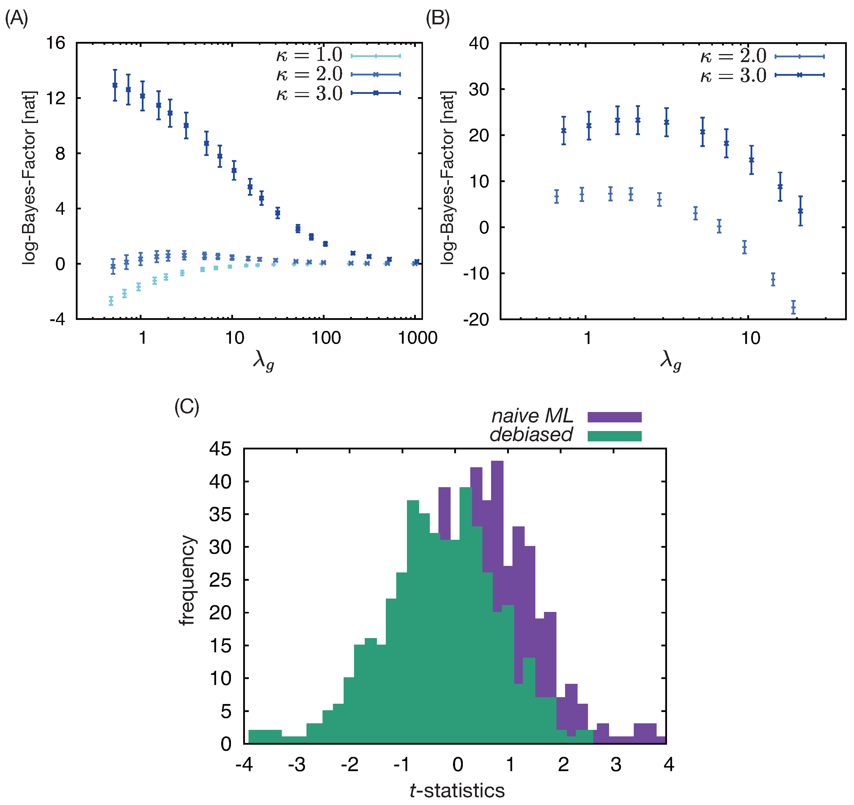
We first performed analysis with only observed covariates , not using latent variables. Here, we assumed . In the validation of assumptions, the inclusion of the time elapsed after enrollment in the set of covariates improved BME (Figure 3(A)), suggesting that the enrolled subjects are heterogeneous, presumably due to an unobserved factor. Then, we analyzed the dataset with a latent variable, maximizing the marginal log-likelihood with EM algorithm (see e.g., Chapter 9 of Ref.[23]), which led to further improvement of BME (Figure 3(B)). In this calculation, we observed that the optimization becomes numerically unstable for small presumably because of the singularity of the model. We examined the estimated values of with 500 datasets generated by the identical process with different seeds for its random-number generator, and the results confirmed that the suggested debiased estimators identify the ground truth with minimal bias, in contrast with the naive ML estimator (Figure 3(C)).
4. Discussion
Preceding studies [3,4,5] showed that the Cox model allows multiple, contradictory interpretations. In the present study, we therefore proposed to estimate hazard ratios of treatment options in an exponential hazard model with or without latent variables that lacks baseline hazard as a function of time elapsed after enrollment. We assumed that conditional hazard should not depend on a specific time during the observation, and measured the degree of its violation as an indicator of the necessity to seek additional covariates or latent variables. Given this and several other testable assumptions as well as conventional assumptions for causal inference in observational studies, we clarified the context in which the estimated hazard ratios are causally interpreted. Then, we proposed methods to debias ML estimators of hazard ratios in cases with and without latent variables, simultaneously validating the model assumptions by calculating BME. Numerical simulations confirm that the proposed method allows us to systematically identify necessary variables and estimate the treatment effect with minimal bias.
Epidemiologists and statisticians might find it psychologically difficult to abandon the Cox models with baseline hazard because of its established role as a default model. The popularity of the Cox model is due to its semiparametric nature. Leaving the aspects of data difficult to model as a blackbox is an attractive idea. Furthermore, the Cox’s MPL estimator [35] for log-hazard ratios of treatment groups is asymptotically efficient [36,37], which is a natural consequence of obviating the estimation of the baseline hazard (thanks to the cancellation in the representation of partial likelihood). Because of this asymptotic efficiency, all other estimators, including the ML estimator, have essentially been reduced to theoretical subjects, while a relatively small number of studies have suggested the advantage of using the others (e.g. [22,38]). The present results suggest the need to reconsider this situation by reevaluating the tradeoff between the efficiency and uninterpretability due to the indefinite baseline hazard. The disadvantage of using MPL is not only the uninterpretability. First of all, the indefinite baseline hazard is impossible to interpret from the physical and biological points of view. No physical process depends on the time elapsed after the enrollment. Thus, its use is solely justified by convenience. However, from a technical point of view, comparing the estimation of in the present study and the inverse-probability-of-treatment weight for marginal structural Cox models used for a similar purpose [18], one can see that the former is a marginal estimand in terms of time and hence usually easier to estimate. The standard method for the latter, that is, estimating the transition probability of treatment and censoring for each value of covariates and each time t, possibly works better in a simple model setting, such as analysis involving only a few–several discrete variables. However, carrying this out under the nonlinear effect of a high-dimensional covariate is prohibitive. In fact, the recently proposed application of doubly robust estimation to marginal structural Cox models are still limited to simple model settings to which machine learning cannot be incorporated [39]. This is why we could not directly compare the results with our method and the conventional method based on the marginal structural Cox model. Another negative factor for MPL approach is that the combination of Bayes theorem and partial likelihood is only approximately justifiable, so extending Cox regression to Bayesian settings is not straightforward, although efforts in this direction have been made for Cox models as well [40]. Considering these negative factors for the MPL approach, we conclude that the debiased ML approach should be reconsidered in causal inference for observational studies with uncontrolled dynamic treatment and real-time measurement of a large number of covariates.
In technical aspects, for the sake of clear exposition, we restricted our study to a relatively simple setting, in which only non-informative right censoring is considered, only a single binary treatment variable can take the value of one, and only a single time-independent latent variable is allowed. For the first condition, the advantage of ML estimation has been demonstrated in the context of informative censoring [41]. Therefore, extending our framework in this direction seems promising. Second, the use of multiple independently changing treatment variables is straightforward, but requires cumbersome modifications, where finding the root of scores amounts to solving multivariate algebraic equations of degrees greater than one. To apply our framework to models with continuous treatment variables, the conditional distribution of treatment assignment for each value of covariates must be identified in a manner similar to what is done with propensity scores for continuous treatment [42]. There is still a technical challenge in this step, because machine learning of the conditional distribution of continuous variables remains in the phase of theoretical argument (see e.g., Refs.[43,44]), not practical use. The extension of our framework to models with multiple (possibly continuous, time-dependent) latent variables would face the identifiability problem. Although progress has been made in both theoretical analysis of identifiability [45,46,47,48] and numerical examination of identifiability in the context of biological modeling [49], there is still a technical challenge. Related to this topic, using a singular model can lead to effective breakdown of asymptotic normality of estimators [50]. In this case, the framework of debiased machine learning would itself need modifications, and the Laplace approximation of BME also fails and needs to be replaced by Monte-Carlo integration [51] (or information criteria for singular parametric models [52,53]). The above difficulties being mentioned, use of rich classes of latent-variable models for which inference methods have been extensively developed in machine learning (especially those for time-series data [54,55]) is yet an attractive, worthy challenge. In this challenge, our technique to use variational distributions as a nuisance parameter in the orthogonalization will be useful.
Author Contributions
T.H. conceptualized the study. T.H. performed all of the mathematical works in the study. T.H. and S.A. designed models and simulation data. T.H. developed all program codes. T.H. and S.A. interpreted the analyzed results. T.H. wrote the manuscript. T.H. and S.A. have read and agreed to its contents and have approved the final manuscript for submissions.
Funding
This research was supported by the Ministry of Education, Culture, Sports, Sciences and Technology (MEXT) of the Japanese government and the Japan Agency for Medical Research and Development (AMED) under grant numbers JP18km0605001 and JP223fa627011.
Data Availability Statement
All of the source codes that support the findings of this study are available as supplementary materials.
Acknowledgments
We would like to express our gratitudes to two medical IT companies, 4DIN Ltd. (Tokyo, Japan) and Phenogen Medical Corporation (Tokyo, Japan) for financial support, while both companies had no role in the research design, analysis, data collection, interpretation of data, and review of the manuscript, and no honoraria or payments were made for authorship.
Conflicts of Interest
The authors declare no conflicts of interest.
References
- Lin, R.S.; Lin, J.; Roychoudhury, S.; Anderson, K.M.; Hu, T.; Huang, B.; Leon, L.F.; Liao, J.J.; Liu, R.; Luo, X.; et al. Alternative Analysis Methods for Time to Event Endpoints Under Nonproportional Hazards: A Comparative Analysis. Statistics in Biopharmaceutical Research 2020, 12, 187–198. [Google Scholar] [CrossRef]
- Bartlett, J.W.; Morris, T.P.; Stensrud, M.J.; Daniel, R.M.; Vansteelandt, S.K.; Burman, C.F. The Hazards of Period Specific and Weighted Hazard Ratios. Statistics in Biopharmaceutical Research 2020, 12, 518–519. [Google Scholar] [CrossRef] [PubMed]
- Hernán, M.A. The Hazards of Hazard Ratios. Epidemiology 2010, 21. [Google Scholar] [CrossRef] [PubMed]
- Aalen, O.O.; Cook, R.J.; Røysland, K. Does Cox analysis of a randomized survival study yield a causal treatment effect? Lifetime Data Analysis 2015, 21, 579–593. [Google Scholar] [CrossRef] [PubMed]
- Martinussen, T.; Vansteelandt, S.; Andersen, P.K. Subtleties in the interpretation of hazard contrasts. Lifetime Data Analysis 2020, 26, 833–855. [Google Scholar] [CrossRef]
- Martinussen, T. Causality and the Cox Regression Model. Annual Review of Statistics and Its Application 2022, 9, 249–259. [Google Scholar] [CrossRef]
- Prentice, R.L.; Aragaki, A.K. Intention-to-treat comparisons in randomized trials. Statistical Science 2022, 37, 380–393. [Google Scholar] [CrossRef]
- Ying, A.; Xu, R. On Defense of the Hazard Ratio, 2023. 2023; arXiv:math.ST/2307.11971].
- Fay, M.P.; Li, F. Causal interpretation of the hazard ratio in randomized clinical trials. Clinical Trials 2024, 21, 623–635. [Google Scholar] [CrossRef] [PubMed]
- Rufibach, K. Treatment effect quantification for time-to-event endpoints–Estimands, analysis strategies, and beyond. Pharmaceutical Statistics 2019, 18, 145–165. [Google Scholar] [CrossRef]
- Kloecker, D.E.; Davies, M.J.; Khunti, K.; Zaccardi, F. Uses and Limitations of the Restricted Mean Survival Time: Illustrative Examples From Cardiovascular Outcomes and Mortality Trials in Type 2 Diabetes. Annals of Internal Medicine 2020, 172, 541–552. [Google Scholar] [CrossRef] [PubMed]
- Snapinn, S.; Jiang, Q.; Ke, C. Treatment effect measures under nonproportional hazards. Pharmaceutical Statistics 2023, 22, 181–193. [Google Scholar] [CrossRef] [PubMed]
- Cui, Y.; Kosorok, M.R.; Sverdrup, E.; Wager, S.; Zhu, R. Estimating heterogeneous treatment effects with right-censored data via causal survival forests. Journal of the Royal Statistical Society Series B: Statistical Methodology 2023, 85, 179–211. [Google Scholar] [CrossRef]
- Xu, S.; Cobzaru, R.; Finkelstein, S.N.; Welsch, R.E.; Ng, K.; Shahn, Z. Estimating Heterogeneous Treatment Effects on Survival Outcomes Using Counterfactual Censoring Unbiased Transformations. 2024; arXiv:stat.ME/2401.11263]. [Google Scholar]
- Frauen, D.; Schröder, M.; Hess, K.; Feuerriegel, S. Orthogonal Survival Learners for Estimating Heterogeneous Treatment Effects from Time-to-Event Data. 2025; arXiv:cs.LG/2505.13072]. [Google Scholar]
- Kennedy, E.H. , H.; Wu, P.; Chen, D.G.D., Eds.; Springer International Publishing: Cham, 2016; pp. 141–167. https://doi.org/10.1007/978-3-319-41259-7_8.Inference. In Statistical Causal Inferences and Their Applications in Public Health Research; He, H., Wu, P., Chen, D.G.D., Eds.; Springer International Publishing: Cham, 2016; Springer International Publishing: Cham, 2016; pp. 141–167. [Google Scholar] [CrossRef]
- Leviton, A.; Loddenkemper, T. Design, implementation, and inferential issues associated with clinical trials that rely on data in electronic medical records: a narrative review. BMC Medical Research Methodology 2023, 23, 271. [Google Scholar] [CrossRef]
- Hernán, M.A.; Brumback, B.; Robins, J.M. Marginal Structural Models to Estimate the Joint Causal Effect of Nonrandomized Treatments. Journal of the American Statistical Association 2001, 96, 440–448. [Google Scholar] [CrossRef]
- Van der Laan, M.J.; Rose, S. Targeted learning in data science; Springer, 2018.
- Chernozhukov, V.; Chetverikov, D.; Demirer, M.; Duflo, E.; Hansen, C.; Newey, W.; Robins, J. Double/debiased machine learning for treatment and structural parameters. The Econometrics Journal 2018, 21, C1–C68. [Google Scholar] [CrossRef]
- Ahrens, A.; Chernozhukov, V.; Hansen, C.; Kozbur, D.; Schaffer, M.; Wiemann, T. An Introduction to Double/Debiased Machine Learning. 2025; arXiv:econ.EM/2504.08324]. [Google Scholar]
- Ren, J.J.; Zhou, M. Full likelihood inferences in the Cox model: an empirical likelihood approach. Annals of the Institute of Statistical Mathematics 2011, 63, 1005–1018. [Google Scholar] [CrossRef]
- Bishop, C.M.; Nasrabadi, N.M. Pattern recognition and machine learning; Vol. 4, Springer, 2006.
- van der Laan, M.J.; Petersen, M.L.; Joffe, M.M. History-adjusted marginal structural models and statically-optimal dynamic treatment regimens. The International Journal of Biostatistics 2005, 1. [Google Scholar] [CrossRef]
- Hille, E.; Phillips, R.S. Functional Analysis and Semi-Groups, 3rd printing of rev. In ed. of 1957. In Proceedings of the Colloq. Publ, Vol. 31. 1974. [Google Scholar]
- Lanckriet, G.R.; Cristianini, N.; Bartlett, P.; Ghaoui, L.E.; Jordan, M.I. Learning the kernel matrix with semidefinite programming. Journal of Machine Learning Research 2004, 5, 27–72. [Google Scholar]
- Bach, F.R. Consistency of the group lasso and multiple kernel learning. Journal of Machine Learning Research 2008, 9. [Google Scholar]
- Meier, L.; Van de Geer, S.; Bühlmann, P. High-dimensional additive modeling. The Annals of Statistics 2009, 37, 3779–3821. [Google Scholar] [CrossRef]
- Koltchinskii, V.; Yuan, M. Sparsity in multiple kernel learning. The Annals of Statistics 2010, 38, 3660–3695. [Google Scholar] [CrossRef]
- Suzuki, T.; Sugiyama, M. Fast learning rate of multiple kernel learning: Trade-off between sparsity and smoothness. The Annals of Statistics 2013, 41, 1381–1405. [Google Scholar] [CrossRef]
- Bach, F.; Jordan, M. Kernel independent component analysis. Journal of Machine Learning Research 2003. [Google Scholar]
- Liu, D.C.; Nocedal, J. On the limited memory BFGS method for large scale optimization. Mathematical Programming 1989, 45, 503–528. [Google Scholar] [CrossRef]
- Williams, C.K.; Rasmussen, C.E. Gaussian processes for machine learning; Vol. 2, MIT press Cambridge, MA, 2006.
- Berlinet, A.; Thomas-Agnan, C. Reproducing kernel Hilbert spaces in probability and statistics; Springer Science & Business Media, 2011.
- Cox, D.R. Regression Models and Life-Tables. Journal of the Royal Statistical Society: Series B (Methodological) 1972, 34, 187–202. [Google Scholar] [CrossRef]
- Efron, B. The Efficiency of Cox’s Likelihood Function for Censored Data. Journal of the American Statistical Association 1977, 72, 557–565. [Google Scholar] [CrossRef]
- Oakes, D. The Asymptotic Information in Censored Survival Data. Biometrika 1977, 64, 441–448. [Google Scholar] [CrossRef]
- Thackham, M.; Ma, J. On maximum likelihood estimation of the semi-parametric Cox model with time-varying covariates. Journal of Applied Statistics 2020, 47, 1511–1528. [Google Scholar] [CrossRef]
- Luo, J.; Rava, D.; Bradic, J.; Xu, R. Doubly robust estimation under a possibly misspecified marginal structural Cox model. Biometrika 2024, 112, asae065. [Google Scholar] [CrossRef]
- Zhang, Z.; Stringer, A.; Brown, P.; Stafford, J. Bayesian inference for Cox proportional hazard models with partial likelihoods, nonlinear covariate effects and correlated observations. Statistical Methods in Medical Research 2023, 32, 165–180. [Google Scholar] [CrossRef] [PubMed]
- Ma, J.; Heritier, S.; Lô, S.N. On the maximum penalized likelihood approach for proportional hazard models with right censored survival data. Computational Statistics and Data Analysis 2014, 74, 142–156. [Google Scholar] [CrossRef]
- Imai, K.; Van Dyk, D.A. Causal inference with general treatment regimes: Generalizing the propensity score. Journal of the American Statistical Association 2004, 99, 854–866. [Google Scholar] [CrossRef]
- Hu, B.; Nan, B. Conditional distribution function estimation using neural networks for censored and uncensored data. Journal of Machine Learning Research 2023, 24, 1–26. [Google Scholar]
- Kostic, V.; Pacreau, G.; Turri, G.; Novelli, P.; Lounici, K.; Pontil, M. Neural conditional probability for uncertainty quantification. Advances in Neural Information Processing Systems 2024, 37, 60999–61039. [Google Scholar]
- Allman, E.S.; Matias, C.; Rhodes, J.A. Identifiability of parameters in latent structure models with many observed variables 2009.
- Allman, E.S.; Rhodes, J.A.; Stanghellini, E.; Valtorta, M. Parameter identifiability of discrete Bayesian networks with hidden variables. Journal of Causal Inference 2015, 3, 189–205. [Google Scholar] [CrossRef]
- Gassiat, E.; Cleynen, A.; Robin, S. Inference in finite state space non parametric Hidden Markov Models and applications. Statistics and Computing 2016, 26, 61–71. [Google Scholar] [CrossRef]
- Gassiat, E.; Rousseau, J. Nonparametric finite translation hidden Markov models and extensions. Bernoulli 2016, 22, 193–212. [Google Scholar] [CrossRef]
- Wieland, F.G.; Hauber, A.L.; Rosenblatt, M.; Tönsing, C.; Timmer, J. On structural and practical identifiability. Current Opinion in Systems Biology 2021, 25, 60–69. [Google Scholar] [CrossRef]
- Watanabe, S. Algebraic geometry and statistical learning theory; Vol. 25, Cambridge university press, 2009.
- Calderhead, B.; Girolami, M. Estimating Bayes factors via thermodynamic integration and population MCMC. Computational Statistics and Data Analysis 2009, 53, 4028–4045. [Google Scholar] [CrossRef]
- Watanabe, S. A widely applicable Bayesian information criterion. Journal of Machine Learning Research 2013, 14, 867–897. [Google Scholar]
- Drton, M.; Plummer, M. A Bayesian Information Criterion for Singular Models. Journal of the Royal Statistical Society Series B: Statistical Methodology 2017, 79, 323–380. [Google Scholar] [CrossRef]
- Moral, P. Feynman-Kac formulae: genealogical and interacting particle systems with applications; Springer, 2004.
- Chopin, N.; Papaspiliopoulos, O.; et al. An introduction to sequential Monte Carlo; Vol. 4, Springer, 2020.
Figure 1.
Two causal graphs describing the causal relationships among the counting process for outcome event, , treatment variable, , covariate, and unmeasured factors, which bifurcate into an actual process and a counterfactual process at time t. Remark 3 discusses how these causal relationships affect the interpretation of the estimation results in the proposed framework.
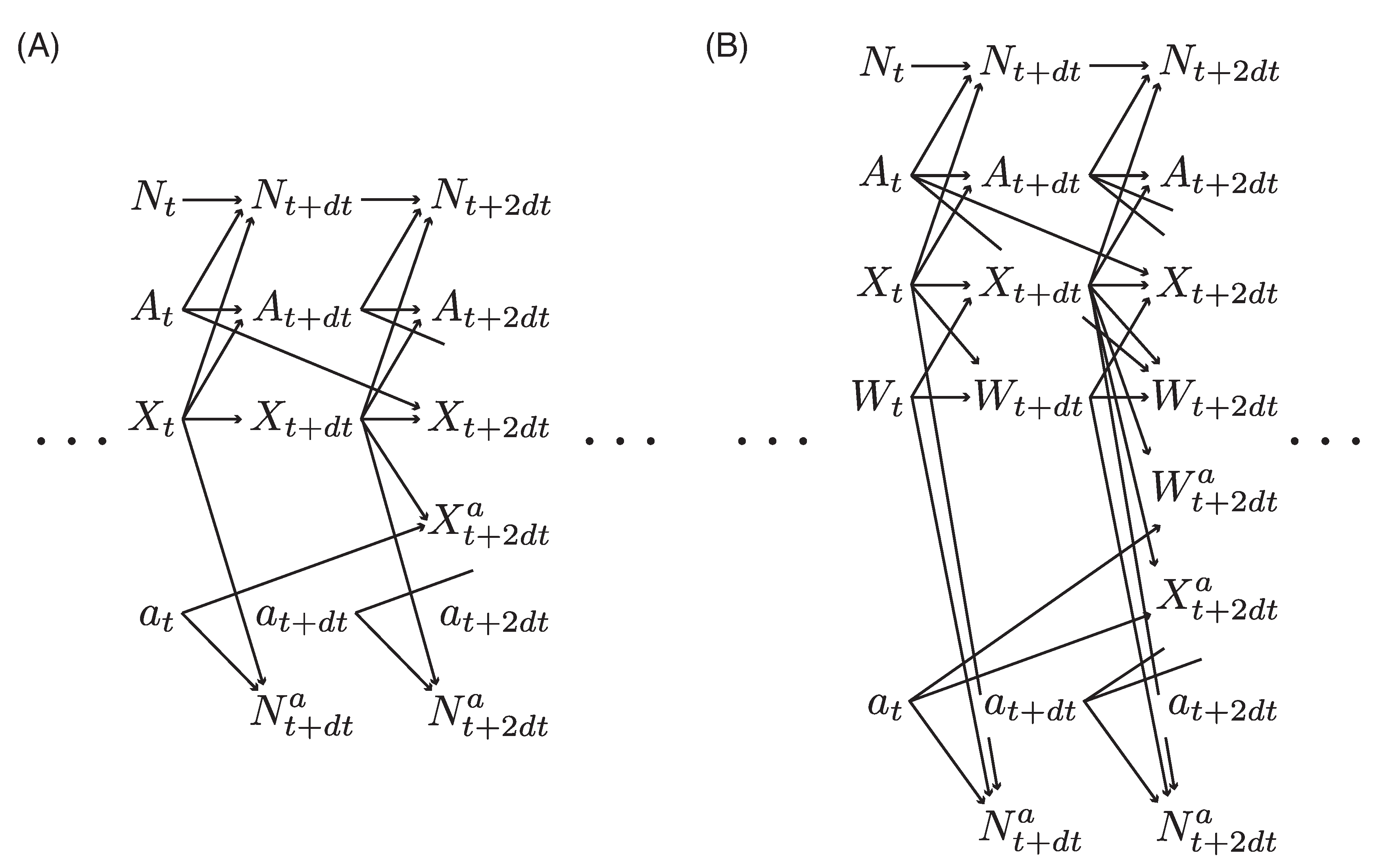
Figure 2.
Numerical results for a clinically plausible data-generation process. (A)–(C): The mean and standard error of the logarithms of the Bayes factors for (A) the correctly specified model and the misspecified models lacking , (B) the misspecified models with or without the inclusion of and (C) the correctly specified models with or without the inclusion of , calculated with ten bootstrap datasets and different regularization parameters . The other hyperparameters are fixed to the optimal values for the smaller model. The log-Bayes factors are calculated by subtracting the log-BME of the larger model from that of the smaller model. (D) and (E): The mean and standard error of (D) log-BME and (E) calculated in the logistic regression for with ten bootstrap datasets and different regularization parameters. (F): The histograms of t-statistics measuring the bias in the naive ML estimator of and the debiased ML estimators of based on nuisance parameter estimated with and , respectively.
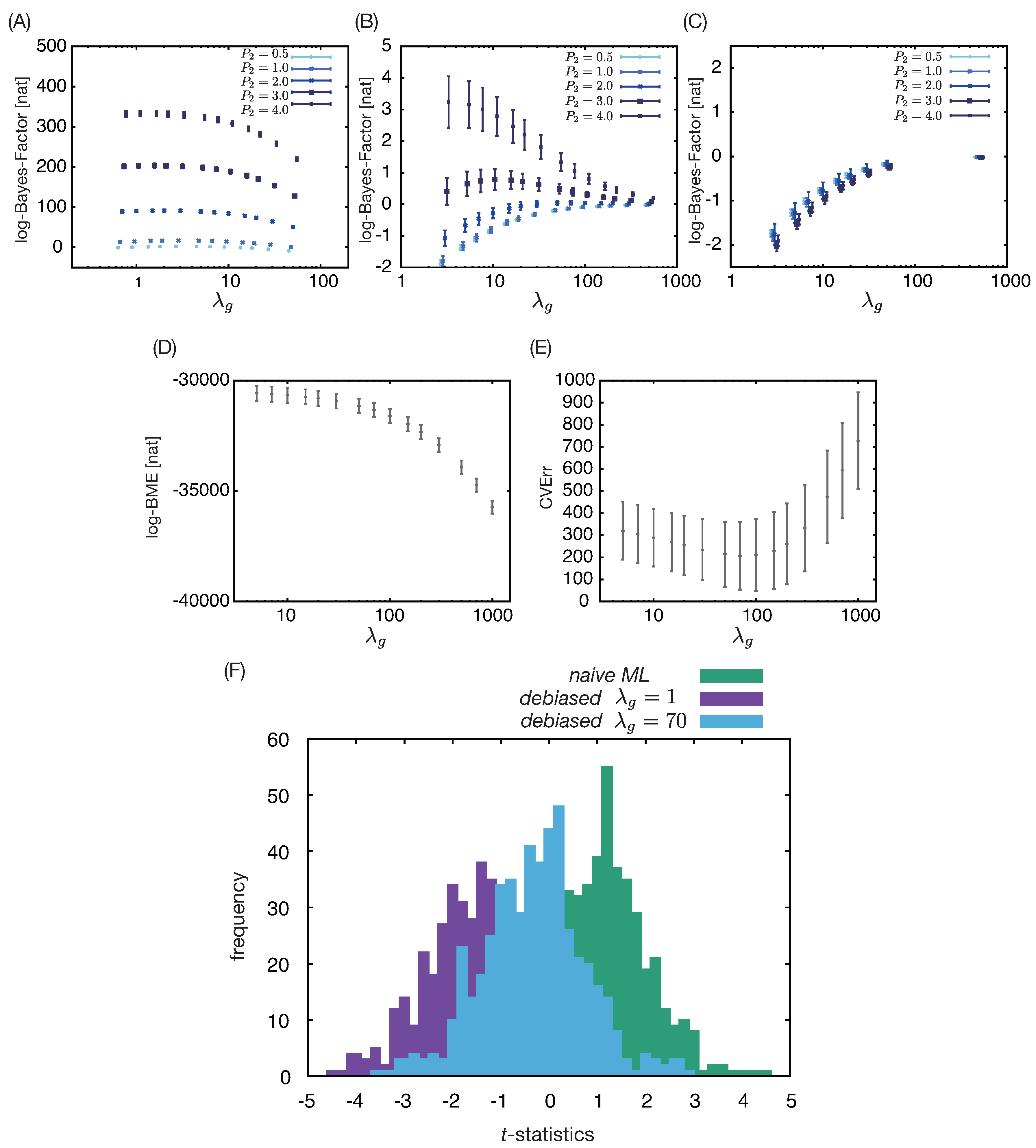
Figure 3.
Numerical results for a clinically plausible data-generation process with a time-independent unobserved factor affecting outcome. (A) and (B): The mean and standard errors of log-BME for (A) the misspecified model with only the observed covariates with or without the inclusion of and (B) the correctly specified model with a latent variable and the misspecified model with only the observed covariates, but without the inclusion of , calculated with ten bootstrap datasets and different regularization parameters for Gaussian kernels. The other hyperparameters are fixed to the optimal values for the smaller (null) model. (C) The histograms of t-statistics measuring the bias in the naive ML estimator of and the debiased ML estimator of based on the correctly specified model with a latent variable.
Disclaimer/Publisher’s Note: The statements, opinions and data contained in all publications are solely those of the individual author(s) and contributor(s) and not of MDPI and/or the editor(s). MDPI and/or the editor(s) disclaim responsibility for any injury to people or property resulting from any ideas, methods, instructions or products referred to in the content. |
© 2025 by the authors. Licensee MDPI, Basel, Switzerland. This article is an open access article distributed under the terms and conditions of the Creative Commons Attribution (CC BY) license (http://creativecommons.org/licenses/by/4.0/).
Copyright: This open access article is published under a Creative Commons CC BY 4.0 license, which permit the free download, distribution, and reuse, provided that the author and preprint are cited in any reuse.


