
Submitted:
23 July 2025
Posted:
25 July 2025
You are already at the latest version
Abstract
Data scarcity and class imbalance pose persistent challenges in cybersecurity AI, par-ticularly for intrusion detection systems, where real-world malicious network traffic is rare and sensitive. To address this, the present study explores the generation of synthetic network traffic using deep generative models, focusing on both Generative Adversarial Networks (GANs) and Variational Autoencoders (VAEs). Building upon recent advances in data synthesis, we introduce a systematic framework for Data Quality Assessment (DQA) to evaluate the realism and utility of generated malicious traffic. Our approach compares the outputs of GANs and VAEs not only in terms of statistical similarity to real attack patterns, but also by measuring their effect on the performance of super-vised/unsupervised Intrusion Detection Models. By embedding synthetic samples into the training process, we quantify improvements in classification accuracy, recall, and robustness under various threat scenarios. The outcomes of this work aim to enhance trust in synthetic data generation techniques, offering reliable augmentation strategies for cybersecurity applications under data-limited conditions.
Keywords:
Data quality
; Cybersecurity
; Data generation
; Gaussian Copula
; CTGAN
; CopulaGAN
; TVAE
; Malicious network traffic
1. Introduction
The continuous advancements of communication technologies, has facilitated the transmission of heterogeneous and multimodal data across different network environments [1]. In addition to this, the proliferation of Internet of Things (IoT) devices has brought about unparalleled levels of connectivity. From laptops, tablets, and smartphones to smart appliances and industrial equipment, an ever-expanding range of devices are continuously producing enormous volumes of data. While this interconnectivity offers important benefits and drives innovation, it also increases the malicious attack surface [2]. Malicious actors swiftly exploit this expanded attack surface targeting vulnerabilities in traditional and IoT devices [3]. Some examples of attacks launched by malicious actors include malware dissemination [4], botnet attacks [5], zero-day exploits [6], and man-in-the middle (MitM) attacks [7]. The cost of cybercrime at a global level is expected to increase from 9.22 trillion dollars in 2024 to 13.82 trillion dollars in 2028 [8]. The cost of a single data breach is also growing. During 2024 a data breach cost 4.88 million dollars on average, 10% higher than the average cost in 2023 [9].
Based on the above, the effective tackling of cyberattacks and more specifically of the detection of network intrusion attempts is crucial. Modern technologies like Artificial Intelligence network intrusion models are highly dependent on quality training data. In this light, the augmentation of existing or newly collected data is an active research topic which constantly evolves. Generative Adversarial Networks (GANs) which were introduced by Ian Goodfellow et al [10] in 2014 have the ability to generate almost identical data records to those provided as inputs. More specifically, GANs use two competing neural networks: a generator creates synthetic data samples, while a discriminator tries to distinguish them from real data. Through this adversarial training, the generator learns to produce highly realistic synthetic data that mimics the original dataset's distribution, thereby expanding and diversifying the training set for improved model performance. Thus, GANs can prove quite effective and useful for applications that require data augmentation.
Variational Autoencoders (VAEs) are another emerging generative technique for data augmentation, especially in data-intensive applications. VAEs were first introduced by Kingma and Welling in 2013 [11] and further explained by the same authors in 2019 [12]. Similarly, to the GANs described earlier the VAEs are comprised of two linked models: an encoder (recognition model) that approximates the latent posterior distribution for the decoder (generative model), enabling Expectation Maximization-style learning. Following this procedure a VAE is able to sample from this distribution and generate new, synthetic data points that are similar to the original training data.
In this study the focal point is the data augmentation of Network Intrusion Detection Systems (NIDS). The promising capabilities of GAN and VAE technologies enable the research community to lift existing barriers that posed from data scarcity and inadequate data quality to the field of cybersecurity and specifically for network intrusion detection. By examining both GAN and VAE technologies and their performance for the data generation task, useful insights are provided that can aid future research to better align efforts for synthetic data generation and augmentation which can be used as training data in NIDS. In this light, four different synthesizers were employed and the data generated from them evaluated based on a set of different metrics. Those data synthesizers are:
- GaussianCopula
- CTGAN
- Tabular Variational Autoencoder (TVAE)
- CopulaGAN
This study evaluates the synthesizer efficiency and synthetic data quality based on comprehensive fidelity and similarity metrics using the CICIDS2017 dataset [13] as original data. The goal is to determine the optimal approach for this specific task by assessing both data similarity and generative performance.
The remainder of the paper is organized as follows: Section 2 presents related works, focusing on the domain of cybersecurity and mainly revolving around GANs, (T)VAEs and the combination of them. Section 3 describes in detail the proposed methodology designed and developed, whilst Section 4 elaborates on the produced results. Finally, Section 5 concludes the paper.
2. Related Works
GANs have been extensively used in scientific literature for addressing scarcity or imbalance of datasets related to NIDS can be found in scientific literature. Zhao et al. [14] implemented three different GAN models (i.e., Conditional Tabular GAN, Vanilla GAN, and Wasserstein GAN) for augmenting datasets related to NIDS. The authors then compared the performance of two classification models (Random Forest - RF and Decision Tree – DT), when trained on the original CICIDS2017 [13] dataset, and when trained with the CICIDS2017 dataset which had been augmented, using the aforementioned GAN models. The improvement was very important, reaching even flawless classification scores (recall, precision and F1 scores equal to 1). More specifically, the precision was improved by 13%, the recall was improved by 35% and the F1-score was improved by 30%. Rao and Babu [15] proposed a GAN-based model for augmenting data related to network attacks. The so-called Imbalanced Generative Adversarial Network (IGAN) model was particularly useful for augmenting minority samples in network traffic datasets and was experimentally tested in combination with an ensemble of Lenet 5 and Long Short Term Memory (LSTM) models. This model yielded better overall accuracy and (over 98%) detection rate of minority attack samples as compared to other contemporary approaches (i.e., Adaboost, Convolutional Neural Networks – CNNs, LSTM, RF, Lunet). Another GAN-based solution for addressing the problem of data imbalance in NIDs-related datasets was proposed by Park et al. [1]. The model was capable of generating realistic data and was combined with Deep Neural Networks (DNNs), CNNs and LSTM classification models for network intrusion detection. Experimental testing on the NSL-KDD [16] and the UNSW-NB15 [17] dataset resulted In accuracies of 93.2% and 87% respectively. Ding et al. [18] proposed another GAN-based model for data augmentation which can be used in imbalanced network traffic datasets. The so-called Tabular Multi-Generator Generative Adversarial Network (TMG-GAN) was capable of generating different kinds of attacks at the same time. It also led to decreased class overlap among the distributions of different generated instances. Experimental testing on the CICIDS2017 led to very satisfactory results of 90.22% precision, 96.38% recall rate, 92.88% F1-score in binary classification, and 99.63% precision, 99.81% recall rate, 99.72% F1-score in multi-classification when combined with a DNN model. These results showed 6,21% better precision, 16.38% better recall rate, and 15.92% better F1-score in multi-classification as compared to the original DNN model.
VAE techniques are also employed in the scientific literature either alone or in combination with GAN techniques for detecting malicious networks events. Yang and Shami [19] proposed an Automated Machine Learning (AutoML) – based autonomous IDS framework which aims to achieve autonomous cybersecurity for next generation (5G and possibly 6G) networks. This approach, similarly to the approach examined in the current study, utilized TVAE technology to enhance data input. More specifically, the study from Yang and Shami engaged an Automated Data Pre-Processing (AutoDP) which automatically detected if there is class imbalance in the input data (CICIDS2017 [13] and 5G-NIDD [20]). When imbalance was detected then the minority classes were enriched with synthetic data samples created by the TVAE engaged. The objective function of the TVAE in this study was the Evidence Lower Bound (ELBO) and the imbalance was detected based on three metrics: the number of classes; the samples per class; and the average number of samples per class. When the number of samples of a class was below a predefined threshold, then this class was enriched with synthetically generated data produced by the TVAE.
Li et al. [21] proposed a method for data augmentation and intrusion detection based on VAE and GAN models. The particular method was capable of generating data instances with predefined labels, leading to a more balanced dataset than the original one. This method was then combined with LSTM and Multi-Scale Convolutional Neural Networks (MSCNNs) for extracting network characteristics and also fused different features for improving the detection rate of malicious events. Experimental testing on the NSL-KDD dataset led to 83.45% accuracy and 83.69% F1-Score. A similar approach was followed by Meenakshi and Karunkuzhali [22] who also combined VAE and GAN technologies. Their main aim of the proposed model was to improve security in Wireless Sensor Networks (WSNs). The Honey Badger Algorithm (HBA) was used for optimizing the Self-Attention-based Provisional Variational Auto-encoder Generative Adversarial Network SAPVAGAN. Experimental testing of the model indicated up to 23.56% higher accuracy and 23.14% computational time as compared to other contemporary approaches (e.g., ECS-WSN-SLGBM [23], ECS-WSN-RNN [24], and ECS-WSN-WOGRU [25]).
GANs and VAE technologies were also combined by Zixu et al. [26] for anomaly detection in IoT networks. The authors followed an unsupervised approach and also focused on privacy preservation. In their model, a sampling pool was implemented on a centralized controller, making use of different generators from individual IoT networks. Experimental testing was done using the UNSW Bot-IoT dataset [27] and three different classifiers were used, i.e., Support Vector Machine (SVM), Recurrent Neural Network (RNN), and Long Short Term Memory Recurrent Neural Network (LSTM-RNN). The highest accuracy and recall rate were achieved by the SVM model (over 99%). A combination of GANs and VAE approaches was also proposed by Senthilkumar et al. [28]. Their model was called Common Intrusion Detection Framework – Variational Autoencoder Wasserstein Generative Adversarial Network- enhanced by Gazelle Optimization Algorithm (CIDF-VAWGAN-GOA). Experimental testing of this model on the NSL-KDD dataset indicated recall rate improvements of 17.58%, 23.18%, and 13.92% as compared to other similar models (i.e., CIDF-SVM [29], CIDF-DNN[30], CIDF-DBN [31]). Computation time improvements were also noticed as compared to the same models (15.37%, 1.83%, and 18.34% respectively). Chalé and Bastian [32] followed a similar approach that encompassed GAN and VAE to create synthetically generated yet realistic data for ML classifiers in the domain of cybersecurity and specifically the network intrusion. Their study examined how different ML classifiers (RF, SVM, MLP and LR) affected when different percentages of synthetically generated data included in the training dataset. Their study indicated that when the proportion of synthetic data contained in the training dataset was up to 50% the performance of the ML classifiers remained unaffected compared to their performance when trained to real data only. However, when the proportion of the synthetic data was above 50% then the performance of the ML classifiers worsened almost linearly following the increase of the synthetic data percentage. So, Chalé and Bastian found that while generative models like CTGAN and TVAE could produce reasonably realistic synthetic cyber data, classifiers trained solely on synthetic data suffered from high false negative rates.
Ammara et al [33] made a thorough study in which they compared the performance of statistical methods and AI based methods for data generation. In their study they utilized the CICIDS2017 and the NSL-KDD datasets as input data for synthetic data generation. Their comparison is based on four main pillars, i.e., the fidelity (statistical similarity metric), the utility (performance accuracy metric), the class balance, and the scalability. Following their experiments the statistical methods (ROS, SMOTE, ADASYN, Cluster Centroids) showed exceptional results in class balance maintaining 0% difference with the real data however they struggled to capture and produce synthetic data with complex traffic structures. The generative AI models showed better generative capabilities but with trading off in fidelity, utility and computational cost. More specifically, the best performance captured by CTGAN and CopulaGAN with utility (accuracy) over 95% for both datasets engaged. On the other hand, TVAE indicated good performance for the NSL-KDD dataset but struggled with the CICIDS2017 dataset. Saka et al [34] also utilized CTGAN, CopulaGAN and TVAE and examined their performance and efficiency when it comes to generate synthetic data based on CICDDOS2019 [35] dataset. Based on similarity metrics, accuracy metric for ML classifiers and class balance. All three methods – CTGAN, CopulaGAN and TVAE – presented similar performance when it comes to similarity metrics (Pearson Correlation, Spearman Correlation, Cosine Similarity, Euclidean Distance) with the TVAE showing better performance when it comes to class balance. On the other hand, when it comes to Classification Accuracy, different ML classifiers tested using data generated CTGAN and CopulaGAN (above 90%) indicated better performance compared to data generated by TVAE (varying values from 70% to 93%).
Another crucial aspect in addition to the enhancement of available labelled data in the network intrusion and cybersecurity domain refers to privacy concerns that emerge when using network traffic data. In this light, Kotal et al [36] proposed the KiNETGAN which aimed to generate synthetic data from custom collected lab network data (originating from the authors’ laboratory network) and the UNSW-NB15 dataset. Their framework was evaluated against other existing generative AI methods, namely CTGAN [37], OCTGAN [38], PATE-GAN [39], TABLEGAN [40], and TVAE [37], using statistical distance metrics, i.e. Earth Mover’s Distance (EMD) and combination of L1 norm or Manhattan distance to calculate the distance for categorical variables and the L2 norm or Euclidean distance to calculate the distance for continuous variables. Moreover, they evaluated the KiNETGAN in terms of utility results and more specifically using the accuracy metric of different ML classifiers when using the synthetically generated data from all the aforementioned approaches. KiNETGAN demonstrated comparable and promising results both in statistical distance metrics and utility results achieving the best performance in distance metrics together with the CTGAN and outperforming most of the other methods in utility results (average accuracy 81%). It is worth mentioning that KiNETGAN added value is focused on privacy preservation by showing the best performance when it comes to re-identification attack, membership and attribute inference attacks.
The related works studied in this section highlight the potential of generative models like GANs and VAEs to improve intrusion detection by addressing data imbalance and answering to lack of labelled data in this domain. Building on existing knowledge presented before, the next section presents the methodology for this study, detailing the dataset used, the selected models, the evaluation criteria, and the experimental design.
3. Methodology
Chapter 3 presents the methodological approach used to assess the quality and utility of synthetic malicious network traffic generated by deep generative models. The focus of the study lies in a comparative evaluation of four synthesizers, namely, the GaussianCopula [41] representing statistical generative models, CTGAN [42], [37] a deep generative adversarial network model tailored for tabular data, TVAE [43], [37] a variational autoencoder designed to handle mixed type tabular datasets, a deep generative adversarial network model tailored for tabular data, and CopulaGAN [44], [37] a hybrid model that combines statistical techniques with deep generative learning. Through a series of controlled experiments, these models are trained on real malicious traffic data, and the extracted synthetic datasets are evaluated using various quantitative metrics and visual diagnostic tools. These evaluations encompass statistical similarity, likelihood-based measures, detection-based scores, machine learning efficacy assessments, privacy checks and qualitative visualizations. The methodology ensures that each synthesizer is evaluated consistently across the same datasets and under comparable experimental conditions.
3.1. Dataset and Preprocessing Steps
3.1.1. Dataset Description
The experimental analysis in this study is based on the CICIDS2017 [13] dataset, a comprehensive intrusion detection benchmark developed by the Canadian Institute for Cybersecurity (CIC). The dataset was specifically designed to address the limitations of previous intrusion detection datasets by providing realistic traffic patterns, diverse attack scenarios and a complete set of network flow features suitable for anomaly-based detection research.
The dataset comprised five consecutive days of captured network traffic, recorded between 3rd and 7th of July, 2017, within a fully configured network environment that included a variety of operating systems (Windows, Ubuntu, Mac OS) and both benign and malicious activities. The attacks covered a broad range of categories, including Brute Force (FTP, SSH), DoS, DDoS, Heartbleed, Web Attacks, Infiltration and Botnets, executed across different network nodes and scenarios. The dataset includes both full packet captures (PCAPs) and labeled network flow summaries extracted using CICFlowMeter, resulting in a rich feature set of over 80 flow-based attributes per record. The CICIDS2017 dataset initially consisted of approximately 2,099,316 records, encompassing both benign and various categories of malicious network traffic.
Given the scope of this study, which focuses on the generation and evaluation of synthetic malicious traffic for intrusion detection purposes, only malicious instances were selected for further analysis. This filtering step was essential to ensure that the generative models exclusively learned patterns associated with attack behaviors, without interference from benign traffic features and characteristics. The malicious dataset, after this consideration, served as the standardized input for all subsequent preprocessing, model training and evaluation phases described within this study. To this end, 100,000 malicious records were carefully filtered and selected to maintain a representative distribution across the various attack categories, ensuring both data diversity and training feasibility.
3.1.2. Preprocessing Procedure
The initial dataset comprised a total of 87 features, where a wide range of network flow statistics, header attributes, flag counters and time-based measurements had been captured. However, many of these features were either redundant, exhibited high multicollinearity or provided little discriminative power for generative modeling purposes. Particularly, features related to per-packet statistics, fine-grained timing intervals, flag counts with constant values and bulk transfer metrics were excluded to reduce dimensionality and minimize noise that could adversely affect the training of generative models. The final feature set was selected based on domain knowledge, relevance to traffic characterization and their overall contribution to the variance of the dataset. The final dataset comprised a total of 19 attributes plus the target labels column which were retained, as they provided a balanced combination of flow-level statistics and essential protocol indicators, ensuring a representative and manageable input for both synthetic data generation and subsequent evaluation actions.
To ensure consistency and compatibility with the selected synthesizers, the dataset has undergone a structured preprocessing pipeline, as summarized below:
- Feature Selection and Cleaning: Non-informative columns, such as identifiers (Flow ID), source/destination IP addresses, port numbers, and timestamps have been removed. These attributes have been considered irrelevant for pattern-based analysis and could introduce unnecessary noise or risk of memorization.
- Handling Missing and Infinite Values: Instances containing non-available (NaN) or infinite values have been addressed by either imputation or removal, depending on their frequency and overall impact. Columns with excessive missing values have been excluded.
- Normalization of Numerical Features: Continuous numerical features have been normalized to a common scale, using the Min-Max scaling method. This step ensured a balanced contribution of all features during the generative model training.
- Final Dataset Format: The extracted dataset has been structured as a flat table with mixed numerical features and void of identifiers or timestamp dependencies. This standardized format ensures direct applicability to all selected synthesizers in a fair comparative setting.
The preprocessed dataset serves as the unified input for all subsequent generative experiments, ensuring that each synthesizer is evaluated under identical conditions with the same feature space and data distribution. Table 1 presents a summary of the key feature types included within the preprocessed dataset.
3.2. Generative Models Description
The core of this study revolves around evaluating synthetic data generation capabilities based on the selected three models (synthesizers), as described within the introduction of this Chapter. These models are representative of different approaches to tabular data generation, ranging from classical statistical methods to deep learning-based architectures. By leveraging different models with varying theoretical foundations, this work aims to provide a comprehensive comparative quality assessment of the extracted generated results.
The following subsections outline the selected four synthesizers, their underlying methodologies, and the key configuration parameters considered during experimentation.
3.2.1. Gaussian Copula Synthesizer
The GaussianCopula Synthesizer [41] is a statistical model that captures dependencies among variables by modeling their joint distribution using copulas. This approach transforms marginal distributions into a standard normal space, fits a Gaussian copula to the transformed data and then samples synthetic records by reversing the transformation. Its main strength lies in its computational efficiency, interoperability, and ability to capture linear and non-linear dependencies between different variables.
As a purely statistical method, this synthesizer serves as the baseline model in the comparative study implemented within this study. Given its deterministic nature, it offers limited parameter tuning, primarily related to data handling and sampling strategy.
3.2.2. CTGAN Synthesizer
The CTGAN Synthesizer [42] is a commonly known deep generative adversarial network (GAN) designed specifically for tabular data. Unlike traditional GANs, CTGAN employs a conditional generation mechanism that addresses challenges unique to structured datasets, including imbalanced categorical distributions and mixed data types. This algorithm introduces mode-oriented normalization techniques and conditional vector sampling to improve learning stability and sample diversity.
CTGAN includes several tunable hyperparameters that influence its learning abilities, such as the number of Epochs, the number of Batch size, the architecture/dimensions of the generator network (hidden layers) and the architecture of the discriminator network.
During the experiment phase on Chapter 4, these parameters are systematically varied to observe their impact on synthetic data quality generation.
3.2.3. TVAE Synthesizer
The TVAE Synthesizer [43] is based on the Variational Autoencoder (VAE) framework, adjusted for tabular data generation. VAEs learn a latent space representation of the input data through an encoder-decoder architecture, enabling the generation of new data samples by sampling from the latent space. TVAE handles mixed-type data and supports conditional sampling processes, making it suitable for structured datasets with both categorical and continuous variables. The key tunable parameters of TVAE include: the number of epochs, the batch size, the architecture of the encoder and the decoder networks. As with the CTGAN, the experiments are conducted with parameter variation to evaluate the performance and sensitivity of the generated data samples.
3.2.4. CopulaGAN Synthesizer
The CopulaGAN Synthesizer [44] combines both statistical modeling with deep learning throughout the integration of copula-based data transformations with GAN training. This hybrid approach aims to leverage the strengths of both methodologies, including the dependency capturing of copulas and the generative flexibility of GANs.
During this study, its inclusion provides an additional comparative perspective, especially regarding the trade-off between interpretability and generative capacity.
3.2.5. Summarization of Model’s Configurations
Each synthesizer is trained independently on the preprocessed malicious traffic dataset under identical experimental conditions. Hyperparameters are systematically varied in a controlled manner to assess their influence on the synthetic data generation process. Table 2 summarizes the key configuration parameters for each synthesizer considered within this study.
3.3. Experimental Setup
During the experimental phase of this study, the design has been structured to systematically evaluate the behavior of each synthesizer under predefined and controlled conditions. By applying uniform data preparation and training procedures as outlined in sub-chapter 3.2, the objective is to ensure a fair comparison across the selected generative models. This section details the training protocol, configuration variations and the synthetic data generation process employed in the study.
3.3.1. Training Steps and Practices
The training phase constitutes a critical part of the current experimental methodology, during which each synthesizer learns the statistical properties and dependency structures of the real network traffic dataset. To ensure fairness and consistency, all models are trained individually on the same preprocessed dataset described in Section 3.2. No additional filtering, sampling or feature transformation has been applied beyond what was performed during the preprocessing stage.
Each synthesizer utilizes its own internal training mechanism, as detailed and implemented within the SDV library [45]. For deep generative models, specifically for the CTGAN, TVAE and CopulaGAN Synthesizers, the training procedure involves iterative optimization using stochastic gradient descent methods. The models update their parameters in response to the reconstruction level or adversarial losses computed over each batch of data, aiming to capture both marginal distributions and inter-feature relationships as presented within the input dataset.
On the other hand, the GaussianCopula Synthesizer employs a statistical fitting approach without iterative training. It estimates marginal distributions and dependency structures directly using copula transformations and multivariate normal modeling, producing a deterministic model after a single fitting pass over the data.
To ensure stability and repeatability, each training run has been initialized with a random seed controlled where possible. Furthermore, all synthesizers are trained until they complete the predefined number of epochs (in the case of deep models) or until the fitting process converges (for the statistical-oriented GaussianCopula model). In the post-training stage, the fitted models are saved and used exclusively for synthetic data generation in the subsequent evaluation phase.
This consistent training methodology ensures that the comparison across the four different models focuses on the inherent qualities of the synthetic data they produce, without interference from differences in data preparation or inconsistent training practices.
3.3.2. Hyperparameter Variation Experiments
A fundamental step of this study is to assess and analyze the capabilities and limitations of each generative model in correlation to the variation of its configuration parameters. To this end, a series of controlled experiments are conducted in which selected hyperparameters are systematically varied for the deep generative models. This approach allows the study to analyze not only the performance of each model under default settings but also their sensitivity to different architectural and training configurations.
The primary parameters selected for variation include the number of training epochs, the batch size and the network dimensions of key model components (such as generators and discriminators for the GAN models, encoders and decoders for the TVAE model). These parameters have been chosen due to the fact that they directly affect the model's learning dynamics, convergence behavior and its ability to generalize from the input data without observing overfitting or underfitting phenomena. By varying them systematically across predefined ranges, the study aims to capture a holistic view of each model's generative performance spectrum.
As previously noted, the GaussianCopula model does not require hyperparameter variation, as it relies on deterministic statistical fitting without iterative training. In this study purposes, this model serves primarily as a baseline reference point for comparative purposes.
Table 3 summarizes the hyperparameter configurations selected for the experimental analysis.
3.4. Data Generation Procedure
Following the completion of the training phase for each synthesizer, synthetic datasets have been generated for evaluation purposes. This step of synthetic data generation is considered quite critical, since it directly reflects the learned ability of each model to reproduce the statistical and structural properties of real network traffic datasets.
For each trained model and configuration, synthetic samples are generated using the respective model sampling method. The following principles are applied in a uniform way, across all experiments to ensure comparability across them:
- Sample Size Matching: The number of synthetic records generated for each configuration is set equal to the size of the real dataset used during training. This matching ensures a fair basis for statistical comparison and metric computation.
- Feature Space Consistency: The synthetic dataset maintains the same dimensionality and feature types (numerical and categorical) as the original, preprocessed one. This consistency ensures that all evaluation metrics, especially those based on statistical tests and deep learning (DL) models, can be applied directly without additional preprocessing.
- Sampling Repetition: To account for randomness inherent in deep generative models, such as weight initialization and sampling variability, each configuration parameterization has been executed in three independent sampling runs. This approach mitigates the impact of outlier detection and supports the assessment of model robustness.
- Post-Generation Processes: The synthetic datasets are inspected for data integrity, ensuring that generated samples do not contain invalid values (e.g., non-available/NaN or infinite values). If such cases have been detected, they are addressed following the same handling or removal strategy applied during the preprocessing stage of the real data.
- Data Preservation for Evaluation: All synthetic datasets have been kept in their raw generated form, without additional transformations applied. These datasets serve as direct input for the evaluation metrics detailed in Section 3.5.
This systematic generation procedure ensures that comparisons between real and synthetic datasets have been based on uniform sample sizes, consistent feature spaces and reproducible results across repeated sampling runs. By following this methodology, the present study aims to maximize the reliability and validity of the data quality assessments on the generated synthetic datasets.
3.5. Evaluation Metrics
The evaluation of the quality of the synthetic dataset can be considered as a multivariate task that requires a combination of quantitative metrics and qualitative analyses. To comprehensively assess the generated synthetic network traffic, this study employs a structured evaluation framework that incorporates statistical fidelity tests, likelihood-based measures, detection-based metrics, utility assessments, privacy checks and visual diagnostics. Each category of metrics targets a particular aspect of data quality, ensuring a holistic evaluation of the generative models’ performance.
Table 4 summarizes the complete set of evaluation metrics employed in this study, categorized by their primary assessment objective.
3.6. Summary of Experiment Execution Workflow
Table 5 provides a summary of the variation experiments and their corresponding parameter configurations. As previously noted, the GaussianCopula Synthesizer does not require parameter variation, since it serves as a baseline with default configuration.
4. Discussion
Chapter 4 includes the evaluation of the statistical quality of the synthetic malicious network traffic generated by the four selected models: GaussianCopula Synthesizer, CTGAN, TVAE, and CopulaGAN. The assessment focuses on the ability of each model to replicate the statistical properties of the real dataset, capturing both marginal distributions and inter-feature dependencies. A set of statistical fidelity metrics-as summarized in Table 4-including distribution similarity measures, correlation analyses and likelihood-based scores, is applied consistently across all models and configurations (Table 5). The evaluation has been structured per model, providing insights into the generative behavior of each approach under the experimental conditions defined in Chapter 3.
4.1. Experimental Dataset Preparations
For the experimental purposes of the proposed synthetic data generation framework, a carefully curated subset of the CICIDS2017 dataset has been implemented. As established within the methodology part, the original dataset contained both benign and malicious network traffic records, totaling 2,099,316 entries. However, since the study focuses exclusively on the generation and quality assessment of synthetic malicious traffic, only attack-related instances have been considered for the experiments.
The initial filtering phase excluded all benign samples, resulting in a malicious-only sample, totaling 516,755 records. Despite its relevance, using the full malicious dataset for training the generative models may pose significant challenges related to computational cost, training convergence, and potential class imbalance issues. Specifically, deep generative models such as GANs and VAEs are sensitive to both the scale and distribution of the input data, often requiring balanced and well-structured datasets for effective learning. Thus, a stratified downsampling approach was applied to the malicious dataset to ensure both representativeness and manageability.
To this end, the malicious samples were grouped by attack type, and up to 10,000 instances per attack category were randomly selected using a controlled random seed for reproducibility. For attack categories with fewer than 10,000 available records, all samples were retained. The extracted balanced malicious dataset comprised a total of 43,176 records, distributed across six distinct attack categories as summarized in Table 6. This balanced dataset was used as the standard input for all subsequent training phases of the generative models and the experimental evaluation presented in the following sections.
4.2. Gaussian Copula Evaluation and Results – Experiment 1 (E1)
The evaluation of the Gaussian Copula model results in Experiment 1 (E1) starts with its statistical fidelity and diagnostic performance. The SDV Diagnostic Tests report perfect scores for Data Validity (100%) and Data Structure (100%), resulting in an overall diagnostic score of 100%, which confirms that the generated synthetic data strictly adheres to the expected schema, feature constraints, and value ranges of the real dataset. However, the SDV Data Quality Assessment yields a lower Column Shapes Score (76.9%) and a Column Pair Trends Score (90.7%), culminating in an Overall Data Quality Score of 83.9%. These results suggest that while Gaussian Copula maintains the integrity of basic structural characteristics, noticeable discrepancies persist in its ability to replicate the detailed statistical relationships of the real data. The overall KS Test Score of 76.9% reflects this average statistical alignment between real and synthetic samples. The outcomes of the Kolmogorov–Smirnov Two-Sample Test further illustrate the limitations of Gaussian Copula in accurately capturing feature distributions. As observed, features such as protocol, icmp code, and icmp type record no significant differences (p-value = 1.0), indicating effective modeling of discrete attributes. Conversely, all continuous features exhibit significant differences (p-value = 0.0000), underscoring persistent challenges in emulating numerical flow characteristics. The Column Shapes Sub-scores reveal a similar pattern: attributes like protocol (97.2%) and icmp code/type (99.9%) achieve high similarity scores, whereas numerical features such as total length of fwd packet (45.7%), total length of bwd packet (38.1%) and flow bytes/s (45.1%) score notably lower. This indicates that Gaussian Copula model struggles particularly with capturing highly variable flow attributes. The down/up ratio (75.3%) also ranks among the weaker-performing features, further confirming the model’s limitations in representing skewed distributions. The detection metrics highlight the distinguishability of Gaussian Copula generated samples from real data. The Logistic Detection score of 78.8% and the SVC Detection score of 87.7% confirm that machine learning classifiers are capable of reliably identifying synthetic data, suggesting a lack of indistinguishability. The TSTR evaluation using a Random Forest Regressor results in a TSTR Score of (0.012, -0.038), indicating a very limited predictive utility when training on synthetic data and testing on real data. Furthermore, at the sample level, the Random Forest classifier reaches a classification accuracy of 99.9%, reinforcing that Gaussian Copula generated data records remain highly distinguishable in supervised learning tasks. These findings collectively suggest that while the Gaussian Copula model generates structurally valid data, its statistical fidelity and practical utility for machine learning applications are constrained. Table 7 summarizes the evaluation results of E1 using the Gaussian Copula model.
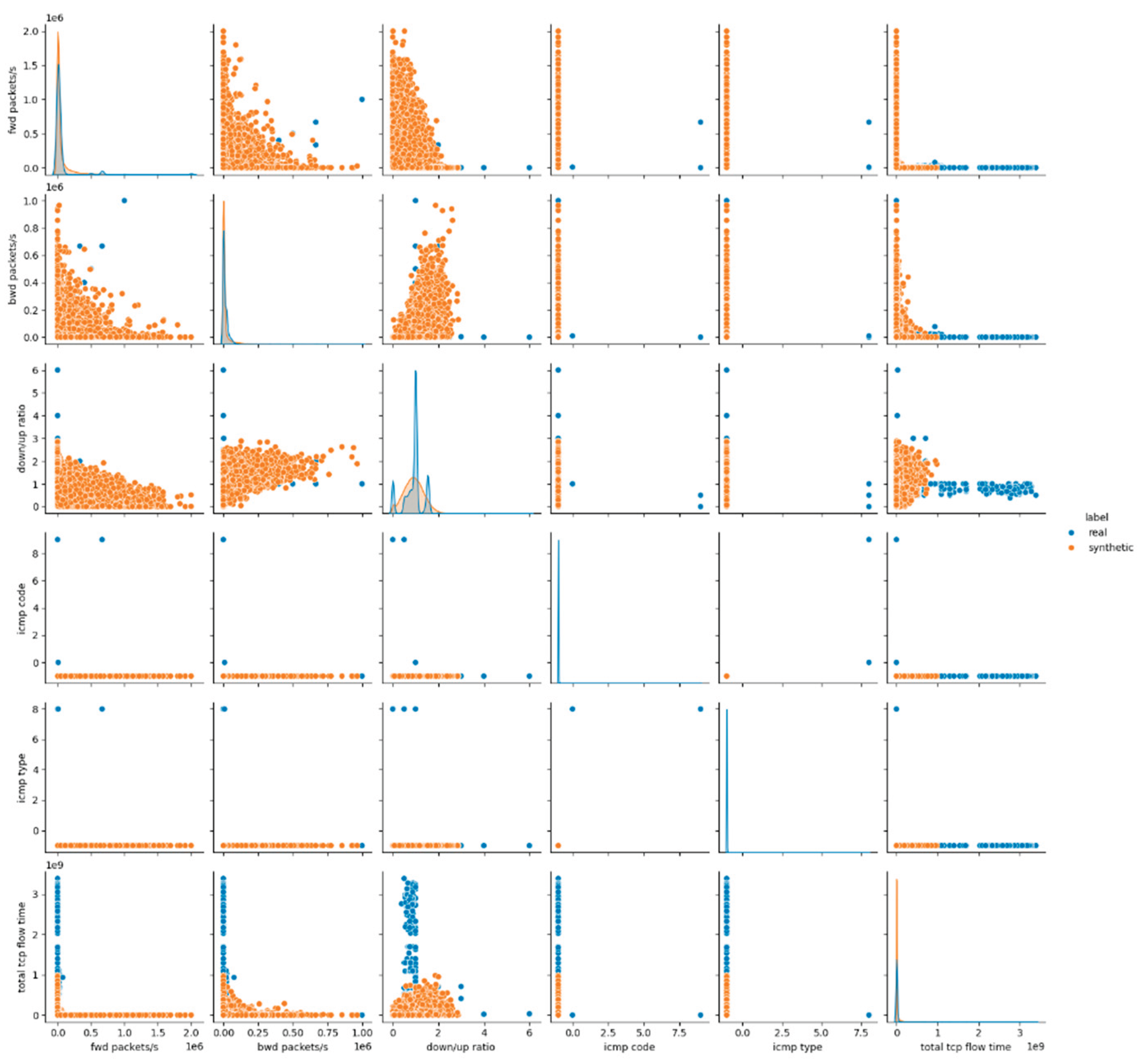
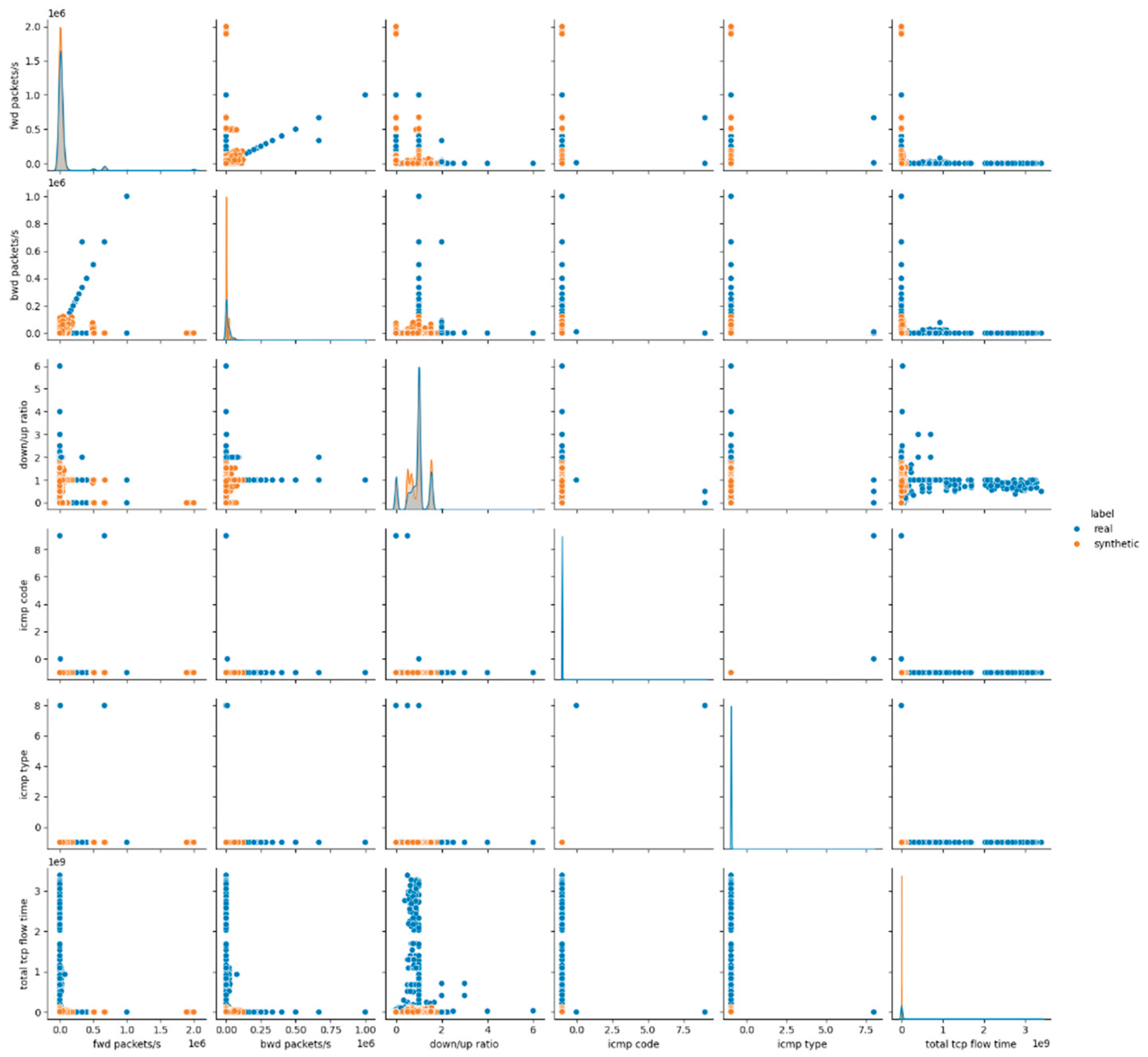
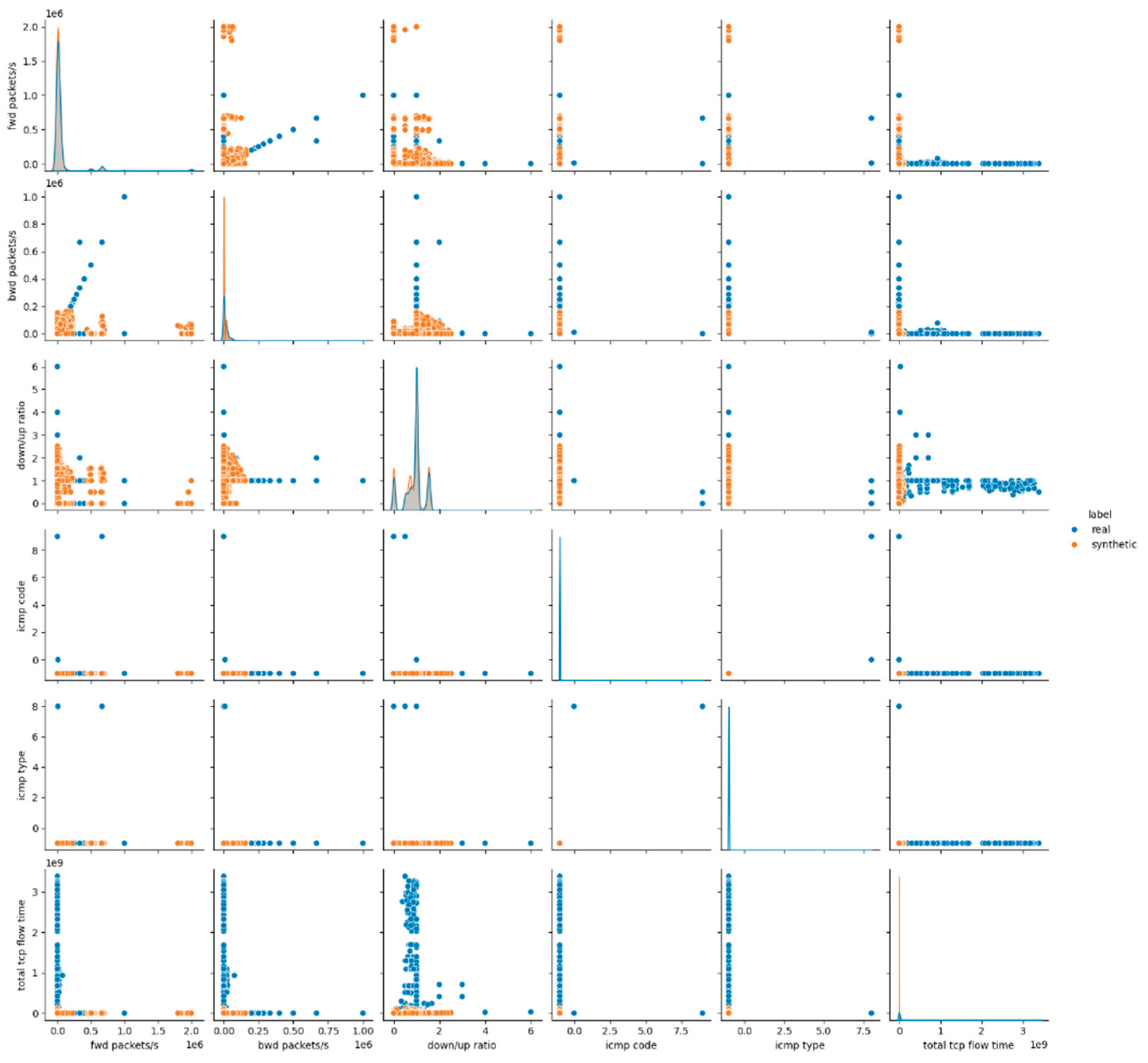
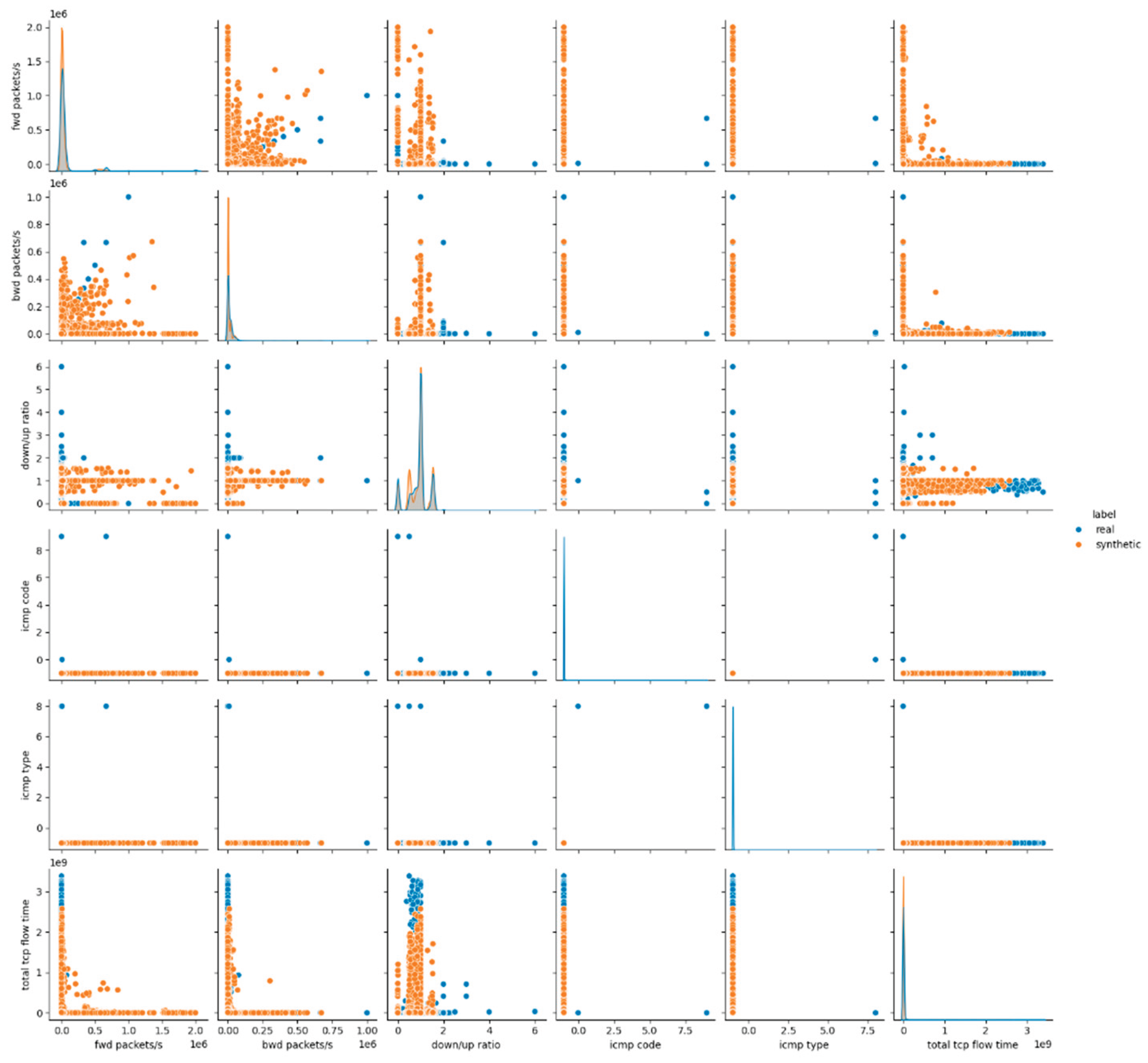
The visual assessment of the synthetic data generated by the Gaussian Copula model further supports the findings of the statistical metrics summarized above. The pairwise feature distribution plots (pairplots) revealed noticeable deviations between the real and synthetic datasets. Specifically, while some attributes such as protocol and icmp type displayed overlapping distributions, continuous numerical features, especially those related to packet sizes, flow durations and rates, showed clear shifts in their distributions. This result suggests that although Gaussian Copula could reproduce marginal distributions of simple numerical (and categorical too) features, it struggled with capturing the complex joint behavior of numerical attributes inherent in the malicious network traffic patterns. Figure 1 presents the results for the first six data features, whereas the remaining results for E1 are provided in Appendix A (Figures A.1 and A.2).
Additionally, the dimensionality reduction visualizations using UMAP projections (Figure 2) provided further insights into the structural differences between the datasets. The synthetic data points formed clusters that were partially overlapping with, but largely distinct from, those of the real data. Unlike models capable of learning higher-order dependencies, the Gaussian Copula generated-samples proved a tendency to cluster more tightly, reflecting the model’s statistical limitations in reproducing the true variance and diversity of the original data. These visual patterns align with the detection and utility metrics, confirming that while the Gaussian Copula maintains certain structural characteristics, it does not fully capture the complexity of real malicious network traffic.
4.3. CTGAN Evaluation and Results
4.3.1. CTGAN - Experiment 2 (E2)
The performance of the CTGAN model in Experiment 2 (E2) has been evaluated through statistical fidelity and diagnostic metrics. The SDV Diagnostic Tests report perfect scores for Data Validity (100%) and Data Structure (100%), resulting in an overall diagnostic score of 100%, which confirms that the synthetic data complies with the schema constraints and contains no structural inconsistencies. However, the SDV Data Quality Assessment yields a Column Shapes Score of 80.9% and a Column Pair Trends Score of 93.2%, with an Overall Data Quality Score of 87.1%. These results indicate that while CTGAN captures most of the dataset’s statistical characteristics, noticeable deviations persist in certain features. The overall KS Test Score of 81.1% reflects a moderate level of statistical similarity between real and synthetic data, slightly lower than that achieved by the baseline model. The results of the Kolmogorov–Smirnov Two-Sample Test provide further insights into CTGAN’s ability to replicate feature distributions. Attributes such as protocol, icmp code, and icmp type show no significant difference (p-value = 1.0) between real and synthetic data, confirming CTGAN’s effectiveness in modeling categorical variables. In contrast, other features record significant differences (p-value = 0.0000), highlighting persistent challenges in capturing the distributions of numerical attributes. The Column Shapes Sub-scores confirm this observation: attributes like total bwd packets (94.6%) and total fwd packet (94.1%) score high, while features such as flow bytes/s (49.6%) and total tcp flow time (65.6%) achieve lower scores. These findings indicate that CTGAN struggles particularly with high-variance flow-related features. The detection metrics further underline the distinguishability of synthetic data. The Logistic Detection score of 78.8% and the SVC Detection score of 87.7% state that classifiers can reliably differentiate between real and synthetic samples. In terms of predictive utility, the TSTR evaluation using a Random Forest Regressor results in a TSTR Score of (-0.035, -0.002), reflecting a limited ability of models trained on synthetic data to generalize to real data. Additionally, the sample-level classification accuracy of 99.9% highlights that CTGAN-based generated samples remain easily identifiable in supervised learning tasks. Overall, these results confirm that while CTGAN improves the modeling of certain data aspects compared to Gaussian Copula model, it still faces notable challenges in producing highly realistic synthetic network traffic. Table 8 presents the evaluation results of E2 using the CTGAN model.
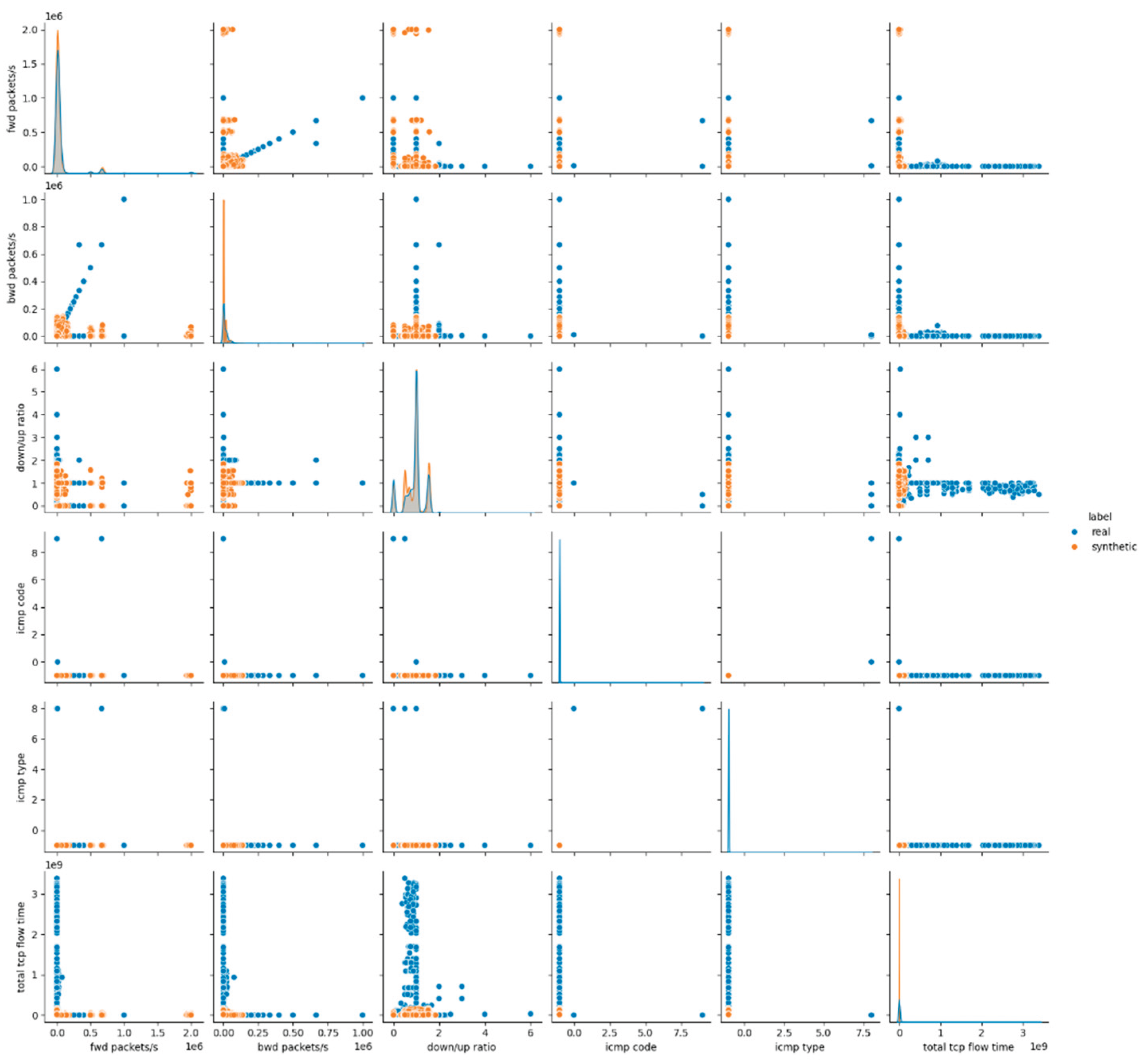
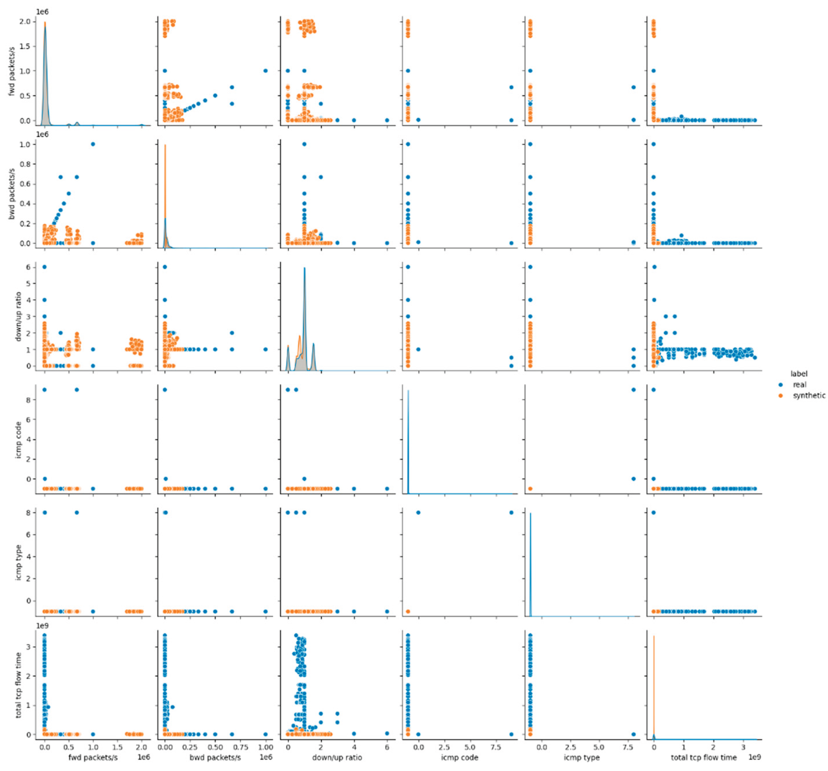
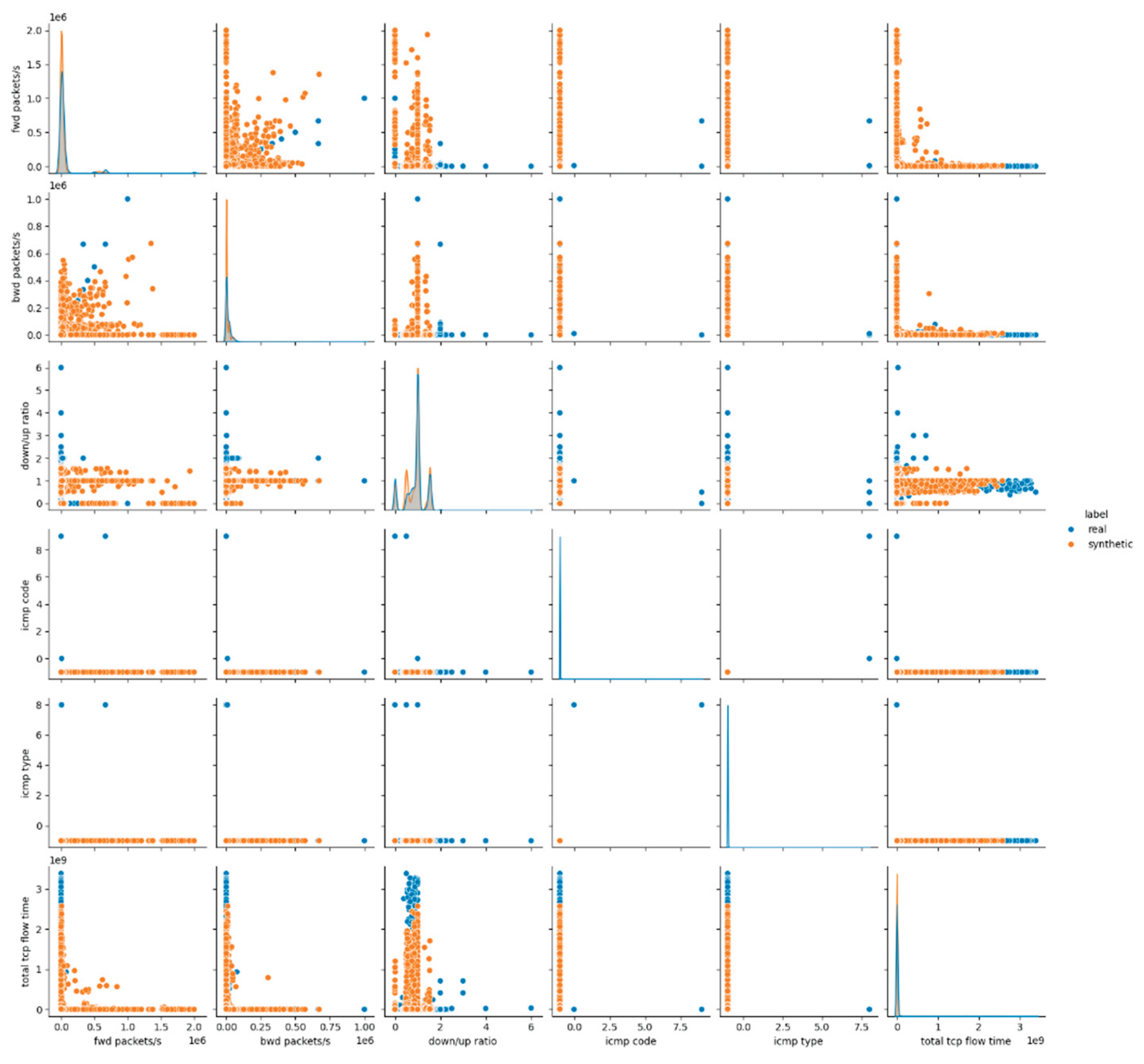
The visual inspection of the CTGAN-generated dataset supports the findings derived from statistical metrics. The pairwise feature distribution plots in Figure 3 and Figures A.3, A.4 in Appendix A, demonstrate mixed behavior: attributes maintain overlapping distributions between real and synthetic data, whereas continuous numerical features exhibit notable shifts and distinct clustering patterns. These deviations are especially evident in flow-related features, where CTGAN fails to reproduce the natural variance and dispersion of the real dataset.
Furthermore, the UMAP projection-depicted in Figure 4-reveals partially overlapping clusters, with several synthetic clusters appearing distinct from those of the real data. This outcome highlights CTGAN’s limited capacity to fully replicate the high-dimensional structure of the original dataset, despite employing a more advanced generative approach compared to GaussianCopula. These visual results align with the statistical analysis and detection metrics, underscoring that while CTGAN enhances certain aspects of synthetic data generation, it remains constrained in reproducing the full complexity of malicious network traffic patterns.
4.3.2. CTGAN - Experiment 3 (E3)
The performance evaluation of the CTGAN in Experiment 3 (E3) started with the SDV Diagnostic Tests which reports perfect scores for Data Validity (100%) and Data Structure (100%), extracting an overall diagnostic score of 100%. This outcome confirms that the generated synthetic data conforms to the expected schema and contains no structural violations. However, the SDV Data Quality Assessment presents a Column Shapes Score of 79.7% and a Column Pair Trends Score of 92.9%, with an Overall Data Quality Score of 86.3%. These results indicate that the selected CTGAN model in E3 successfully captures several key statistical properties of the dataset but also exhibits notable deviations in specific attributes. The overall KS Test Score of 79.7% points to a moderate degree of statistical similarity between the real and synthetic data, comparable to but slightly below the performance of CTGAN model in E2. The Kolmogorov–Smirnov Two-Sample Test results offer further insight into the model’s ability to mimic the distributions of individual features. Discrete variables such as protocol, icmp code, and icmp type show no significant difference (p-value = 1.0), validating the CTGAN’s ability to model categorical data accurately. In contrast, all continuous features report significant differences (p-value = 0.0000), underscoring persistent modeling challenges with numerical attributes. The Column Shapes Sub-scores reinforce this observation: attributes like total bwd packets (95%) and total fwd packet (93.8%) register high scores, whereas features such as flow bytes/s (46.3%) and total tcp flow time (64.9%) present lower similarity. These results highlight that while this model effectively captures some distributional characteristics, it continues to struggle with attributes characterized by high variance or skewed distributions. The detection metrics reflect the continued distinguishability of synthetic samples generated by CTGAN in E3. The Logistic Detection score of 80.6% and the SVC Detection score of 75.3% indicate that machine learning classifiers can still reliably discern synthetic from real data, though with a slightly lower detection capability compared to the baseline Gaussian Copula model and CTGAN in E2. The TSTR evaluation using a Random Forest Regressor results in a TSTR Score of (0.072, -0.003), pointing to limited predictive utility of the synthetic data for downstream tasks. Furthermore, the sample-level classification accuracy of 100% confirms that the generated records remain easily distinguishable when evaluated in supervised learning scenarios. These outcomes imply that despite certain improvements in feature modeling, CTGAN model suggested in E3 shares the same limitations in data realism and utility observed with the other tested synthesizers. Table 9 summarizes the evaluation results of E3 using the CTGAN model.
The visual assessment of the synthetic data produced by the CTGAN model in E3 illustrates the statistical findings discussed above. The pairwise feature distribution plots in Figure 5, Figure A5 and Figure A6 in Appendix A reveal observable discrepancies between the real and synthetic datasets. While categorical variables such as protocol and icmp type maintain overlapping distributions, continuous numerical features, particularly those associated with packet sizes, flow rates, and durations, demonstrate clear divergences. This behavior suggests that although this captures marginal distributions for both the numerical features, it struggles to accurately reflect the joint behavior of numerical attributes inherent in malicious network traffic.
The UMAP projection in Figure 6 further emphasizes these differences in the structural distribution of samples. The synthetic data forms clusters that partially overlap with those of the real dataset but also display distinct separation, highlighting the model's limited ability to replicate the complex, high-dimensional relationships present in the real data. This visual evidence is in line with the detection and utility metrics, confirms that despite its modeling advancements, CTGAN model does not fully emulate the statistical and structural nuances of real malicious network traffic.
4.4. TVAE Evaluation and Results
4.4.1. TVAE - Experiment 4 (E4)
During Experiment 4 (E4) for the TVAE model, the SDV Diagnostic Tests again report perfect scores for Data Validity (100%) and Data Structure (100%), resulting in an Overall Diagnostic Score of 100%. These scores confirm that the generated synthetic data complies with the required schema and contains no structural errors. The SDV Data Quality Assessment yields a Column Shapes Score of 82.6% and a Column Pair Trends Score of 92.5%, culminating in an Overall Data Quality Score of 87.6%. These values suggest that the TVAE model successfully preserves the dataset’s core statistical properties, showing a marginal improvement compared to its previous configuration (E3). The KS Test Score of 82.6% further reflects this trend, indicating a slightly better statistical resemblance to the real data. The results of the Kolmogorov–Smirnov Two-Sample Test highlight the TVAE’s strengths and weaknesses in feature modeling. As seen in previous experiments, discrete variables such as protocol, icmp code and icmp type do not exhibit significant statistical differences (p-value = 1.0), confirming the model’s reliability in capturing specific distributions. On the other hand, all continuous features once again register significant differences (p-value = 0.0000), underscoring the persisting challenge in emulating other types of numerical distributions. The Column Shapes Sub-scores illustrate this inequality: features like total bwd packets (92.8%) and total fwd packet (90.9%) achieve high similarity scores, while attributes such as total tcp flow time (66.7%) and flow duration (73.4%) score lower ones. Despite the improved modeling of several attributes, the TVAE model still struggles with variables marked by high variance or complex distributions. The detection results offer additional insights into the synthetic data's distinguishability. The Logistic Detection Score of 75.5% and the SVC Detection Score of 83.8% suggest that classifiers continue to distinguish between real and synthetic samples with considerable accuracy, while detection scores are slightly reduced compared to earlier experiments. Notably, the TSTR evaluation with Random Forest Regressor records a TSTR Score of (0.918, 0.564), a significant increase over previous experiments, suggesting a noteworthy improvement in the predictive utility of the generated samples. This score implies that models trained on the synthetic data are better able to generalize patterns present within the real data. At the sample level, the Random Forest Classifier Accuracy of 99.9% confirms that individual synthetic data records remain highly distinguishable, reconfirming the challenges in generating samples that are truly indistinguishable from real datasets. Table 10 depicts the evaluation results of E4 using the TVAE model.
The visual analysis of the synthetic data depicted within Figure 7, Figure A7 and Figure A8 (Appendix A) produced by the TVAE model in E4 complements the extracted statistical findings. The pairwise distribution plots reveal a mixed pattern: features such as protocol and icmp type show significant overlap between real and synthetic data, while continuous attributes, especially those related to flow statistics and packet measurements, demonstrate noticeable differences. Although the distributions appear slightly closer than in previous experiments, distinct clustering and scaling inconsistencies remain evident.
The UMAP projection within Figure 8 visualization offers a deeper look into the underlying data structure. Synthetic samples cluster more tightly compared to the more dispersed pattern of real data, while the degree of overlap has slightly increased relative to prior experiments. This partially improved structural similarity hints at some learning of higher-order feature relationships, although significant gaps still exist. These visual outcomes, in combination with the detection and statistical evaluation metrics, confirm that while TVAE in E4 exhibits better performance in certain aspects, it still faces limitations in replicating the full complexity and variability of real malicious network traffic patterns.
4.4.2. TVAE - Experiment 5 (E5)
For Experiment 5 (E5), of the TVAE model, the SDV Diagnostic Tests result perfect scores for both Data Validity (100%) and Data Structure (100%), leading to an Overall Diagnostic Score of 100%. These results confirm that synthetic data completely encounters the structural constraints and schema of the original dataset. The SDV Data Quality evaluation further reports a Column Shapes Score of 85.0% and a Column Pair Trends Score of 92.34%, achieving an Overall Data Quality Score of 89.22%. These scores state that this TVAE model manages to reproduce the underlying statistical patterns of real data with a high degree of fidelity, surpassing several of the previously tested models. The KS Test Score of 84.9% also reinforces this observation, reflecting a strong resemblance in the univariate distributions between the real and synthetic datasets. The Kolmogorov–Smirnov Two-Sample Test provides more granular insights: features such as protocol, icmp code and icmp type show no significant difference (p-value = 1.0), declaring TVAE's reliable modeling of this kind of variables. However, other types of continuous attributes again show significant differences (p-value = 0.0000), highlighting the ongoing challenge of capturing the full complexity of numerical distributions in synthetic data generation. The Column Shapes Sub-scores reflect this pattern, attributes like total bwd packets (95.7%) and total fwd packet (94.1%) perform strongly, while features with higher variability, such as total tcp flow time (68.9%) and down/up ratio (72.4%), achieve ordinary lower scores. The detection metrics reveal that TVAE generated samples are still distinguishable from real data. The Logistic Detection score is 70.8%, and the SVC Detection score reaches 84.1%, indicating that despite the improved data quality metrics, detectable differences remain. Concerning predictive utility, the TSTR evaluation using a Random Forest Regressor yields a positive TSTR Score of (0.918, 0.564), representing one of the highest utility scores in the set of experiments. This result confirms that models trained on synthetic data generated by TVAE can generalize more effectively to real data patterns compared to other tested models. The sample-level classification using Random Forest Classifier confirms the high distinguishability, as reflected by a perfect classification accuracy of 99.9%. Table 11 summarizes the evaluation results of E5 with the TVAE model.
Figure 9, Figure A9 and Figure A10 on Appendix A depict the pairwise feature distribution plots (pairplots) reveal that, while the model successfully captures certain categorical attributes such as protocol and icmp type, discrepancies remain obvious in most continuous-numerical-features. Notably, attributes related to flow dynamics, including flow duration, flow bytes/s and total tcp flow time, show evident distributional shifts between real and synthetic data. Although the overlap in marginal distributions of some simpler features suggests that TVAE during E5 partially succeeds in reproducing single-feature behavior and appears less effective in modeling joint feature interactions, especially those associated with complex network traffic patterns.
As visualized in the corresponding Figure 10 for UMAP projection during E5, synthetic samples form clusters that overlap with those of the real data and still maintain visible separations. This clustering behavior indicates that while TVAE captures certain latent structures and patterns within the data, it struggles to replicate the full diversity and higher-order relationships of the original dataset. The denser clustering of synthetic data points compared to real samples further suggests a tendency toward reduced variance in the generated data.
4.5. CopulaGAN Evaluation and Results
4.5.1. CopulaGAN - Experiment 6 (E6)
For the CopulaGAN model evaluation during Experiment 6 (E6) the built-in SDV Diagnostic Tests provide perfect scores for both Data Validity (100%) and Data Structure (100%), resulting in an overall diagnostic score of 100%. These results confirm that the synthetic dataset adheres to schema constraints and maintains the correct structural integrity without violations. Additionally, the SDV Data Quality metrics report a Column Shapes Score of 89.3% and a Column Pair Trends Score of 95.1%, achieving a high Overall Data Quality Score of 92.2%. These values indicate that CopulaGAN model effectively captures the majority of statistical patterns and inter-feature dependencies from the original dataset, while minor deviations are still present. The KS Complement metric at 89.3% further supports this conclusion, reflecting a generally strong alignment of feature distributions. The Kolmogorov–Smirnov Two-Sample Test results highlight that features like protocol, icmp code, and icmp type result in non-significant differences (p-value = 1.0000), demonstrating CopulaGAN’s reliable handling of these types of variables. However, other attribute types, including flow duration, total tcp flow time and packet-based metrics, show significant differences (p-value = 0.0000). This confirms persistent challenges in generating numerical distributions with high variance. The detailed Column Shapes Sub-scores reflect this behavior: while discrete or simpler features such as protocol (99.9%) and icmp code/type (99.9%) are closely matched, more complex continuous features like down/up ratio (62.8%) remain harder to model accurately. Regarding detection and utility metrics, the model exhibits a Logistic Detection score of 78.8% and an SVC Detection score of 87.7%, indicating that synthetic samples remain distinguishable from real data with high classification accuracy. On the utility side, the TSTR Score of (0.178, -0.074) suggests a marginal predictive capacity when models are trained on synthetic data and tested on real samples. These detection and utility scores align with the statistical assessment, reinforcing the view that despite strong maintenance of structural aspects, CopulaGAN does not fully replicate the complexity required for seamless generalization within downstream tasks. Table 12 summarizes the evaluation results for CopulaGAN in E6.
The pairwise feature distribution plots, in Figure 11, A11 and A12 (Appendix A), reveal a mixed picture. For features, such as protocol and icmp type, the synthetic samples largely overlap with the real data, confirming CopulaGAN's ability to replicate these types of distributions. However, when examining other numerical attributes, particularly flow duration, flow packets/s, total length of fwd/bwd packet and total tcp flow time, distinct deviations emerge. The synthetic data distributions often appear more compact or shifted compared to the real ones, highlighting the model’s limitations in capturing the full variability and joint behavior of flow-related metrics.
The UMAP visualization in Figure 12 further underscores these observations. While the synthetic samples form clusters that broadly overlap with those of the real dataset, distinct grouping patterns and denser synthetic clusters are evident. This outcome suggests that although CopulaGAN approximates certain structural properties of the data, it tends to generate less diverse samples, potentially due to overfitting or constrained learning of the data's underlying complexity. Overall, the visual patterns align with both the detection metrics and statistical tests, ensuring CopulaGAN’s strong but imperfect capability to reproduce the intricate distributions present in real malicious network traffic data.
4.5.2. CopulaGAN - Experiment 7 (E7)
The built-in SDV Diagnostic Tests, during CopulaGAN’s E7, return perfect scores for both Data Validity (100%) and Data Structure (100%), resulting in a flawless Overall Diagnostic Score of 100%. These outcomes confirm that the synthetic data strictly adjusts to the schema rules and structural constraints of the original dataset. The Data Quality assessment via SDV further highlights CopulaGAN's robust performance, achieving a Column Shapes Score of 90.3% and a Column Pair Trends Score of 95.8%, culminating in a high Overall Data Quality Score of 93.1%. These results indicate that the model effectively captures both univariate distributions and further inter-dependencies with a level of accuracy surpassing previous experiments. The Kolmogorov–Smirnov (KS) Test produces a strong similarity score of 90.1%, reflecting CopulaGAN's proficiency in reproducing the statistical characteristics of the real dataset. The detailed Two-Sample KS Test analysis confirms the trend below: variables such as protocol, icmp code and icmp type display no significant differences (p-value = 1.0), while other continuous attributes outcome statistically significant differences (p-value = 0.0000). The Column Shapes Sub-scores align with these findings, features like total bwd packets (96.1%), total length of fwd packet (94.4%) and flow bytes/s (92.6%) demonstrate significant alignment between real and synthetic data. However, certain attributes, particularly down/up ratio (72.1%) and dst port (76.7%), return comparatively lower scores, indicating persistent challenges in capturing distributions for highly variable or skewed features. In terms of detection and utility metrics, the model achieves a Logistic Detection score of 81.3% and an SVC Detection score of 85.8%, stating that real and synthetic samples are still distinguishable with relatively high confidence. Nonetheless, the TSTR evaluation extracts a moderate score of (0.075, -0.045), indicating some capacity of synthetic data to support downstream learning tasks. At the sample level, the Random Forest Classifier records a near-perfect classification accuracy of 99.9%, underscoring the strong label consistency within the generated samples. Table 13 summarizes the evaluation outcomes of CopulaGAN during E7.
The visual assessment of the synthetic data generated in Experiment 7 (E7) using the CopulaGAN model supports the outcomes observed in statistical metrics. The pairwise feature distributions reveal that, compared to the previous experiments, CopulaGAN consistently improves the alignment of synthetic and real data distributions. While features such as protocol, icmp code and icmp type continue to overlap nearly perfectly, continuous numerical features like total fwd packet, total bwd packets and flow duration demonstrate a notably improved correspondence in both density and joint scatter patterns. However, noticeable deviations still persist in attributes involving dynamic network behaviors, such as flow packets/s, flow bytes/s and down/up ratio, which reflect CopulaGAN’s inherent limitations in capturing high-variance numerical features. Figure 13 illustrates the comparison of distributions for the first six features, with the remaining visualizations presented in Appendix A (Figures A.13, A.14).
Additionally, the UMAP-based dimensionality reduction shown in Figure 14 highlights a tighter overlap between synthetic and real data clusters compared to earlier experiments. Although synthetic points still tend to form denser sub-clusters, they associate more naturally with real data points, indicating a more faithful reproduction of global structural patterns. These visual findings align with the improved detection and statistical similarity scores obtained in E7, further confirming that this CopulaGAN model manages to enhance both marginal and joint feature distributions, while still facing challenges in emulating the full complexity of real malicious network traffic data.
5. Conclusions and Future Work
The current study presented a comprehensive evaluation of synthetic malicious network traffic generation using both statistical and deep generative models, with a focus on evaluating their data quality and structural similarity. Through a systematic set of experiments on the improved CICIDS2017 dataset, four representative models, including GaussianCopula, CTGAN, TVAE and CopulaGAN, were analyzed across various hyperparameter configurations. The comparative analysis disclosed particular differences in each model’s ability to replicate the statistical properties and structural characteristics of real malicious network traffic. Gaussian Copula model, serving as a statistical baseline, delivered high structural validity but failed to capture complex numerical patterns, leading to low utility scores and high detectability. CTGAN showed modest improvements in capturing some distributions, while also struggling with numerical attributes and remaining highly distinguishable. TVAE demonstrated better statistical alignment and utility performance, particularly in downstream predictive tasks, but it still faced challenges with complex feature dependencies. CopulaGAN appeared as the most balanced performing model, achieving higher data quality scores and better overlap in visual analyses. Furthermore, the experiments confirmed that hyperparameter variations influenced performance across all models, especially for deep generative approaches. However, CopulaGAN consistently achieved strong results under different configurations, indicating a higher degree of robustness compared to the other models. Despite these findings, none of the evaluated models managed to generate synthetic data completely indistinguishable from real data, particularly under detection and adversarial evaluation metrics. The extracted results highlight both the potential and the limitations of current generative models for realistic malicious network traffic synthesis.
Beyond the comparative findings, this work contributes to the field by establishing a structured evaluation framework that combines statistical, detection, utility and visual metrics into a unified assessment pipeline. The systematic benchmarking conducted here underscores that synthetic data can serve as a valuable augmentation tool but should not replace real data in critical security applications without thorough validation. While the examined models showed varying degrees of success, none of them could fully replicate the complexity and variability of real malicious traffic patterns, especially when analyzed under adversarial detection scenarios.
Future research could explore advanced generative architectures, such as transformer-based models or diffusion mechanisms, that may enhance the realism and utility of synthetic data. Additionally, tailoring models through domain-specific fine-tuning, introducing privacy-preserving mechanisms and testing deployments in real or near-real environments would provide further insights into their practical applicability and usability. Finally, this study lays a solid foundation for ongoing research aimed at refining synthetic data generation techniques for cybersecurity, highlighting their responsible and effective use in both academic research and operational settings and environments.
Author Contributions
Conceptualization, N.P., T.A., E.D and E.A. ; methodology, N.P., T.A, E.D. and E.A.; software, N.P.; validation, N.P., E.A. and E.D.; formal analysis, N.P., T.A. E.D., E.A.; investigation, N.P, T.A. and E.D.; resources, N.P., E.A., E.D. and T.A.; data curation, N.P., T.A. writing—original draft preparation, N.P., T.A. and E.D.; writing—review and editing, E.A., E.D., T.A.; visualization, N.P. and T.A.; supervision, E.A.; project administration, E.A. All authors have read and agreed to the published version of the manuscript.
Funding
This research received no external funding.
Institutional Review Board Statement
Not applicable.
Informed Consent Statement
Not applicable.
Data Availability Statement
The data presented in this study are available on request from the corresponding author.
Conflicts of Interest
The authors declare no conflicts of interest.
Abbreviations
The following abbreviations are used in this manuscript:
| ADASYN | Adaptive Synthetic Sampling Approach |
| AI | Artificial intelligence |
| CIDF | Common Intrusion Detection Framework |
| CNN | Convolutional Neural Network |
| CTGAN | Conditional Tabular Generative Adversarial Network |
| DDoS | Distributed Denial of Service |
| DNN | Deep Neural Network |
| DoS | Denial of Service |
| DQA | Data Quality Assessment |
| DP | Data Pre-processing |
| DT | Decision Tree |
| ELBO | Evidence Lower Bound |
| EM | Expectation Maximization |
| FTP | File Transfer Protocol |
| GAN | Generative Adversarial Network |
| GOA | Gazelle Optimization Algorithm |
| HBA | Honey Badger Algorithm |
| ICMP | Internet Control Message Protocol |
| IDS | Intrusion Detection System |
| IGAN | Imbalanced Generative Adversarial Network |
| IoT | Internet of Things |
| IP | Internet Protocol |
| LR | Logistic Regression |
| LSTM | Long Short-Term Memory |
| MitM | Man-in-the-Middle |
| ML | Machine Learning |
| MLP | Multi-Layer Perceptron |
| MSCNN | Multi-Scale Convolutional Neural Network |
| NaN | Non-Available |
| NIDS | Network Intrusion Detection System |
| PCAP | Packet Capture |
| RF | Random Forest |
| RNN | Recurrent Neural Network |
| ROS | Random Over-Sampling |
| SAPVAGAN | Self-Attention-based Provisional Variational Auto-encoder Generative Adversarial Network |
| SMOTE | Synthetic Minority Oversampling Technique |
| SSH | Secure Shell |
| SVM | Support Vector Machine |
| TCP | Transfer Control Protocol |
| TMG-GAN | Tabular Multi-Generator Generative Adversarial Network |
| TVAE | Tabular Variational Autoencoder |
| VAE | Variational Autoencoder |
| VAWGAN | Variational Autoencoder Wasserstein Generative Adversarial Network |
| WOGRU | Whale Optimized Gate Recurrent Unit |
| WSN | Wireless Sensor Network |
| LD | Linear dichroism |
Appendix A
Experiment 1 (E1)
Figure A1.
Pairwise Feature Distribution Plots (Pairplots) for E1 (dataset features 7-12).
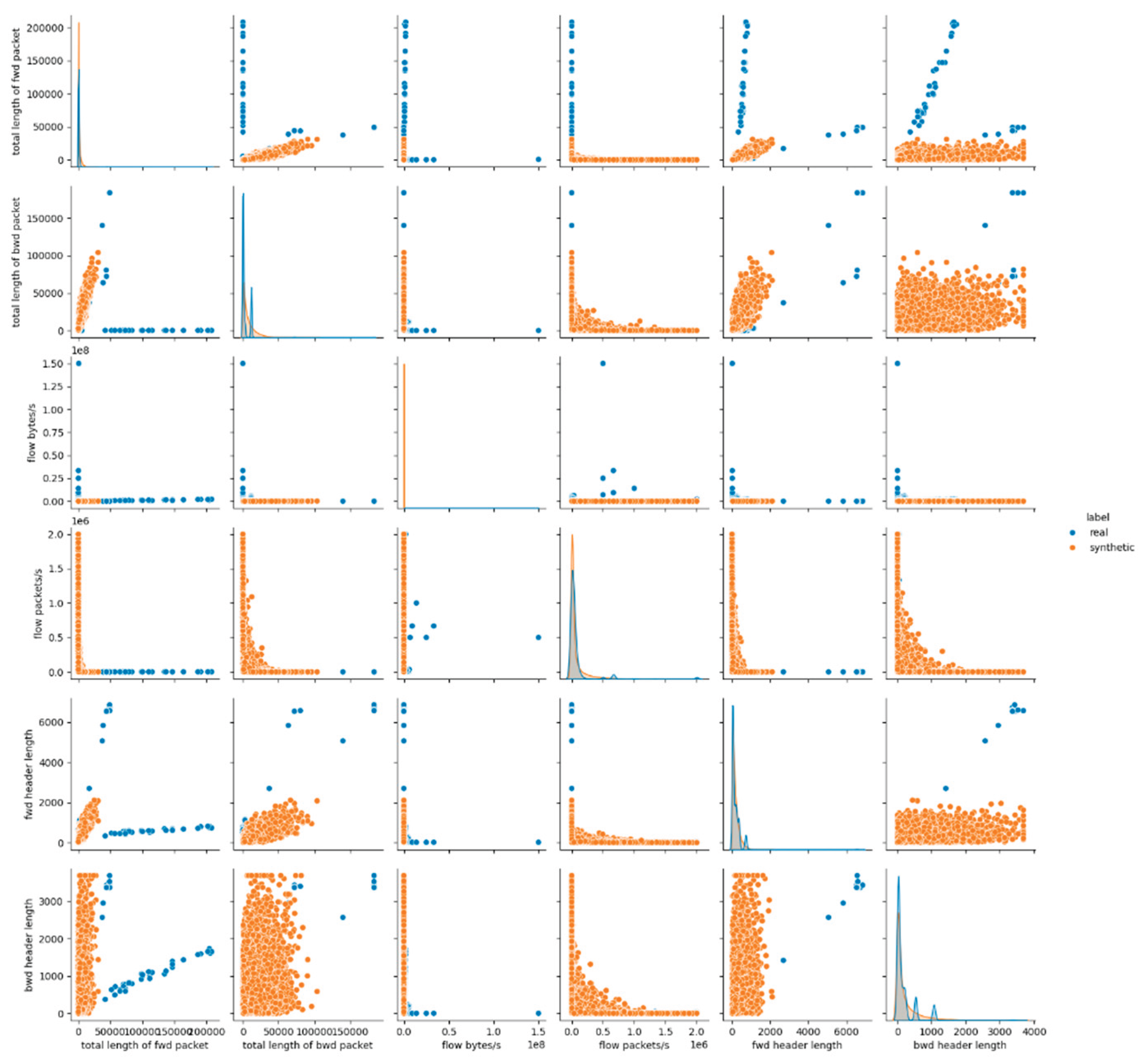
Figure A2.
Pairwise Feature Distribution Plots (Pairplots) for E1 (dataset features 13-18).
Experiment 2 (E2)
Figure A3.
Pairwise Feature Distribution Plots (Pairplots) for E2 (dataset features 7-12).
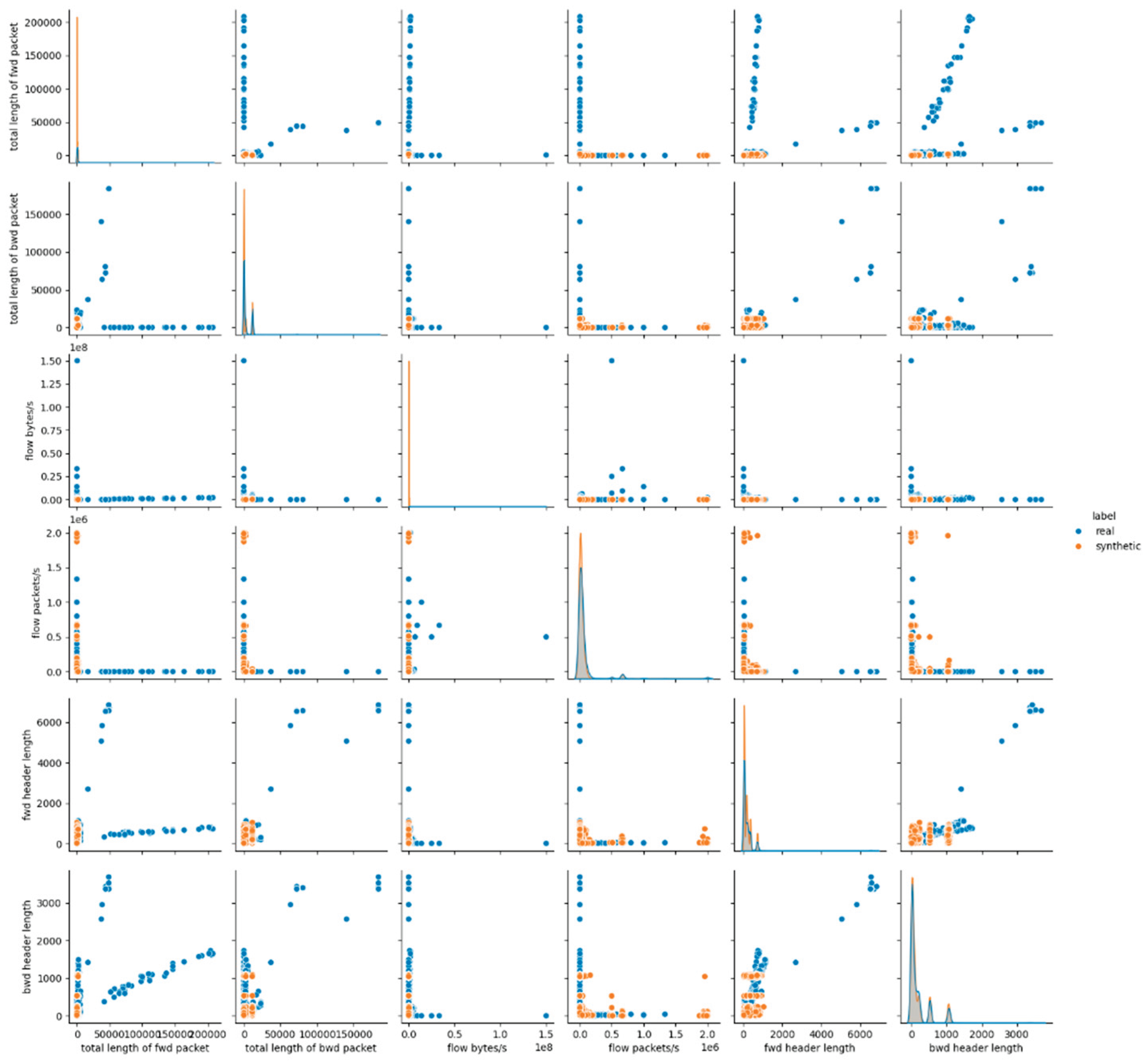
Figure A4.
Pairwise Feature Distribution Plots (Pairplots) for E2 (dataset features 13-18).
Experiment 3 (E3)
Figure A5.
Pairwise Feature Distribution Plots (Pairplots) for E3 (dataset features 7-12).
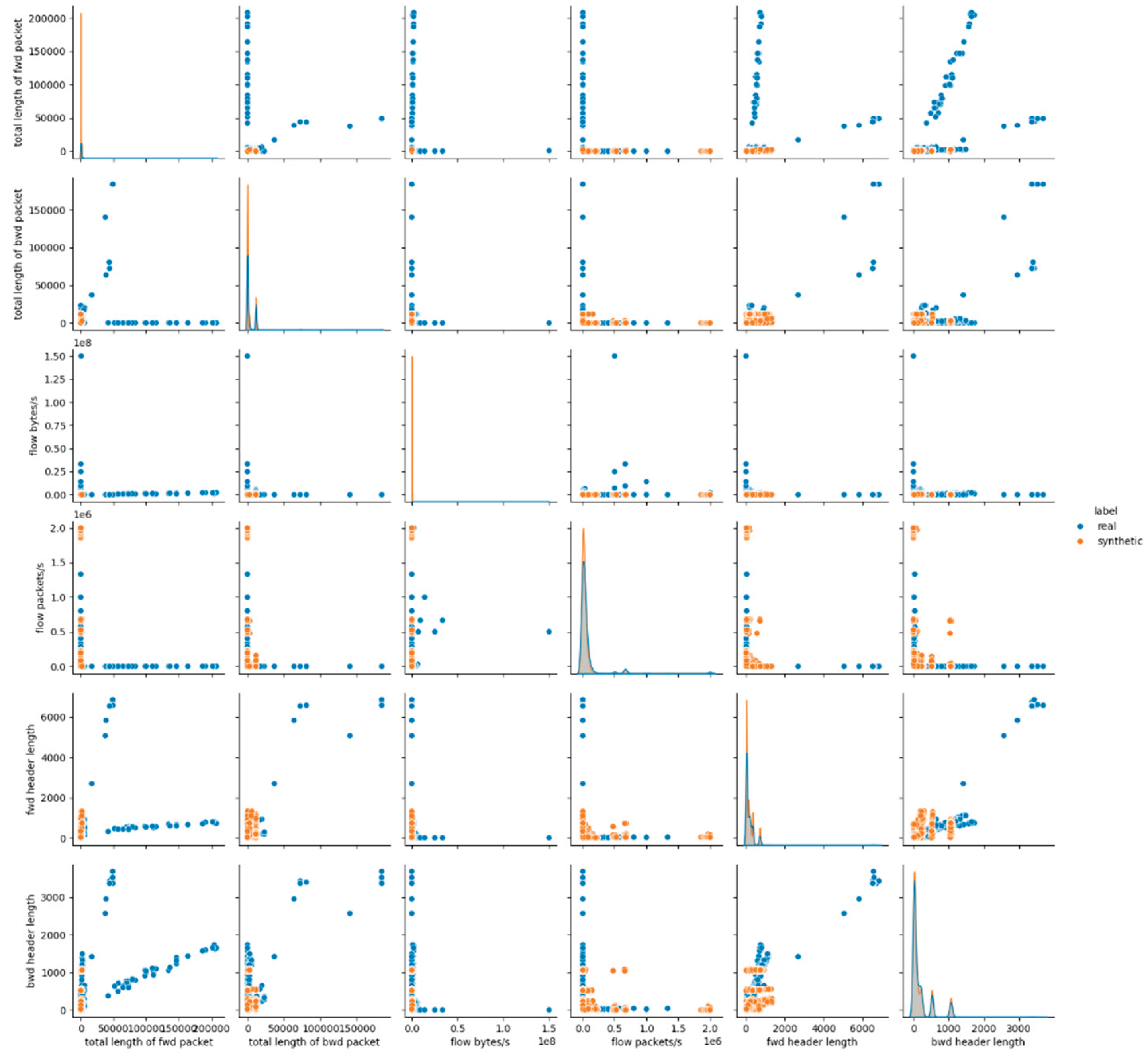
Figure A6.
Pairwise Feature Distribution Plots (Pairplots) for E3 (dataset features 13-18).
Experiment 4 (E4)
Figure A7.
Pairwise Feature Distribution Plots (Pairplots) for E4 (dataset features 7-12).
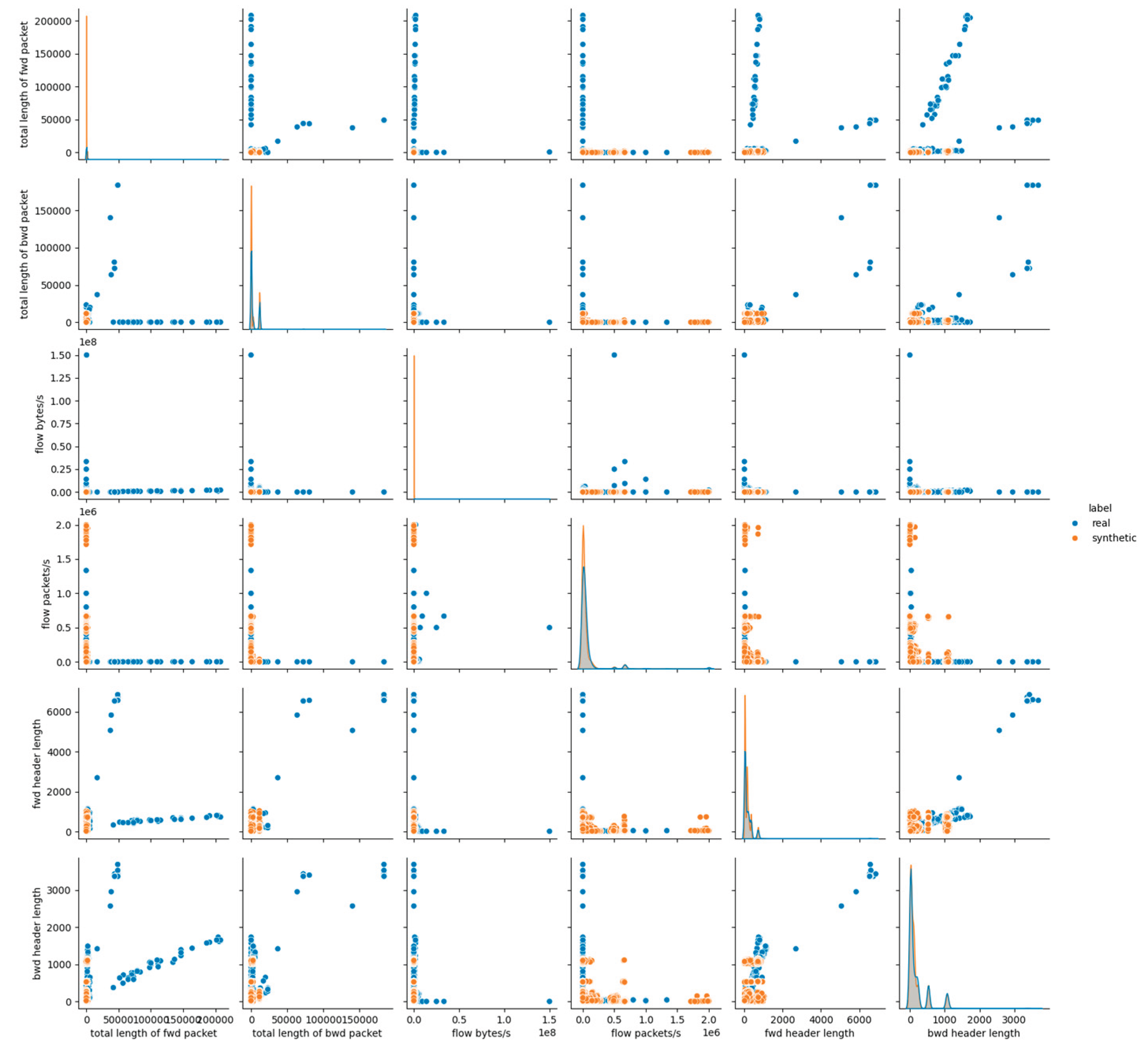
Figure A8.
Pairwise Feature Distribution Plots (Pairplots) for E4 (dataset features 13-18).
Experiment 5 (E5)
Figure A9.
Pairwise Feature Distribution Plots (Pairplots) for E5 (dataset features 7-12).
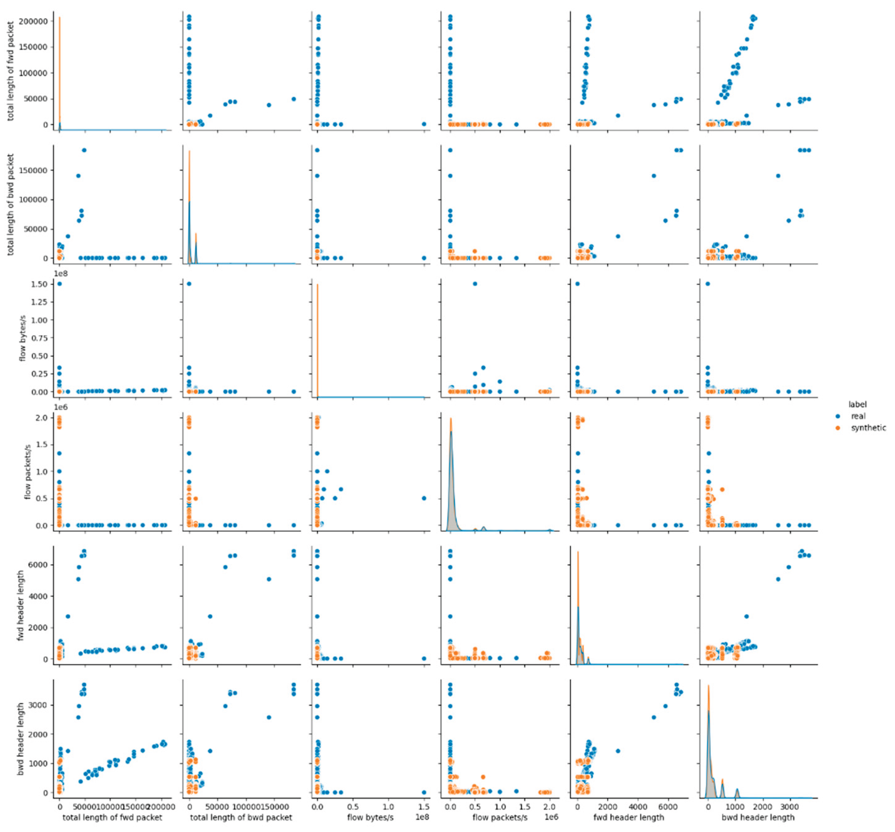
Figure A10.
Pairwise Feature Distribution Plots (Pairplots) for E5 (dataset features 13-18).
Experiment 6 (E6)
Figure A11.
Pairwise Feature Distribution Plots (Pairplots) for E6 (dataset features 7-12).
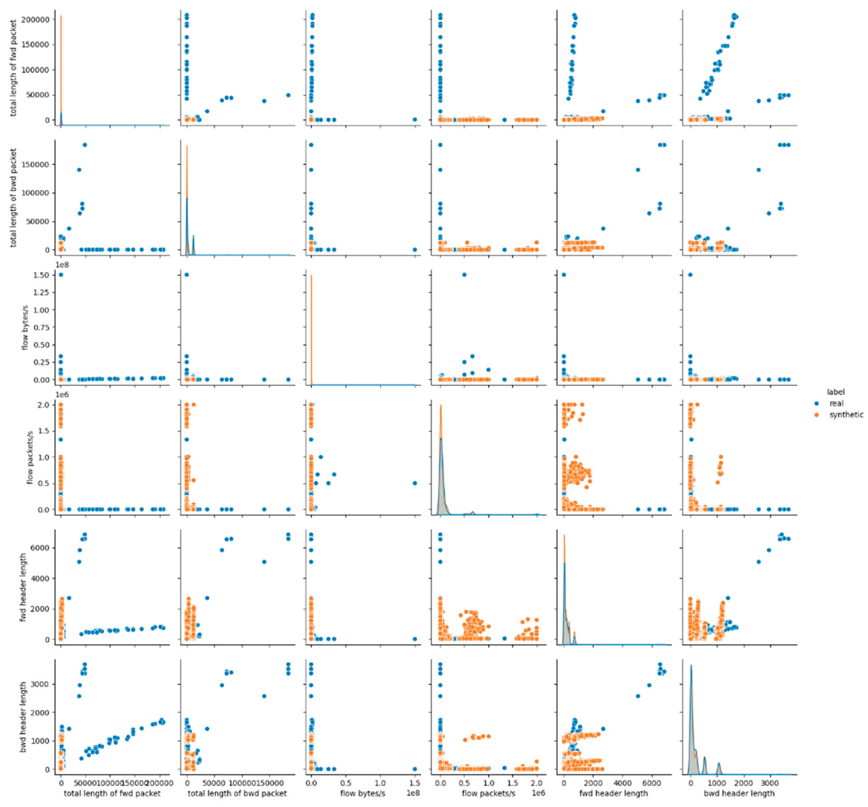
Figure A12.
Pairwise Feature Distribution Plots (Pairplots) for E6 (dataset features 13-18).
Experiment 7 (E7)
Figure A13.
Pairwise Feature Distribution Plots (Pairplots) for E7 (dataset features 7-12).
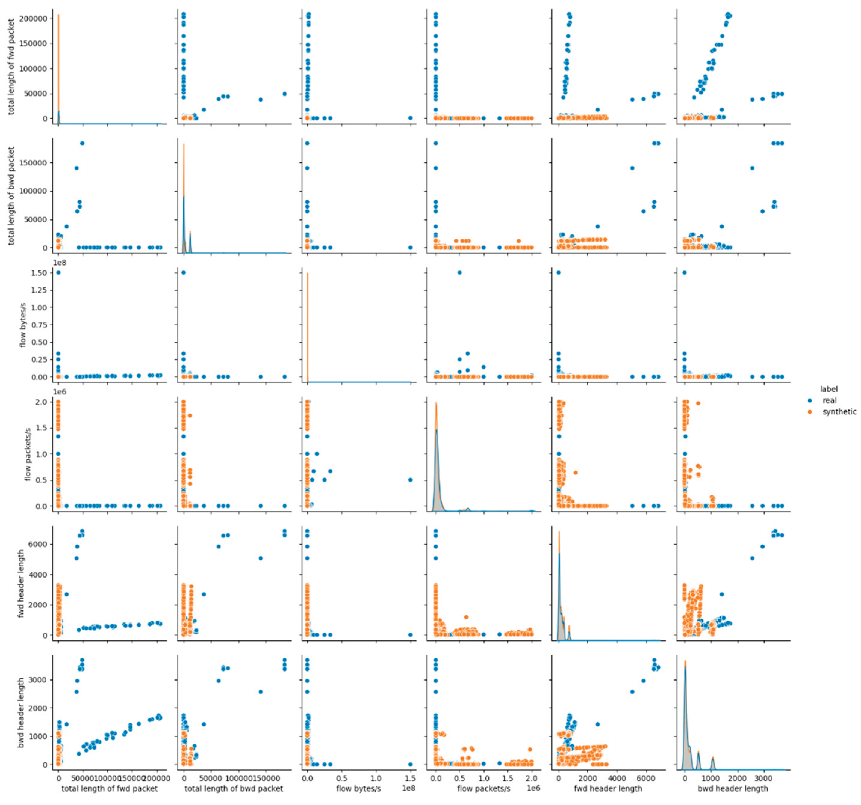
Figure A14.
Pairwise Feature Distribution Plots (Pairplots) for E7 (dataset features 13-18).
References
- Park, C.; Lee, J.; Kim, Y.; Park, J.-G.; Kim, H.; Hong, D. An Enhanced AI-Based Network Intrusion Detection System Using Generative Adversarial Networks. IEEE Internet of Things Journal 2023, 10, 2330–2345. [Google Scholar] [CrossRef]
- Hussain, B.; Du, Q.; Sun, B.; Han, Z. Deep Learning-Based DDoS-Attack Detection for Cyber–Physical System over 5G Network. IEEE Transactions on Industrial Informatics 2021, 17, 860–870. [Google Scholar] [CrossRef]
- Kampourakis, V.; Gkioulos, V.; Katsikas, S. A Systematic Literature Review on Wireless Security Testbeds in the Cyber-Physical Realm. Computers & Security 2023, 133, 103383. [Google Scholar] [CrossRef]
- Piqueira, J.R.C.; Cabrera, M.A.M.; Batistela, C.M. Malware Propagation in Clustered Computer Networks. Physica A: Statistical Mechanics and its Applications 2021, 573, 125958. [Google Scholar] [CrossRef]
- Gelgi, M.; Guan, Y.; Arunachala, S.; Samba Siva Rao, M.; Dragoni, N. Systematic Literature Review of IoT Botnet DDOS Attacks and Evaluation of Detection Techniques. Sensors 2024, 24. [Google Scholar] [CrossRef]
- Zhao, X.; Veerappan, C.S.; Loh, Peter.K.K.; Tang, Z.; Tan, F. Multi-Agent Cross-Platform Detection of Meltdown and Spectre Attacks. In Proceedings of the 2018 15th international conference on control, automation, robotics and vision (ICARCV); 2018; pp. 1834–1838.
- Fereidouni, H.; Fadeitcheva, O.; Zalai, M. IoT and Man-in-the-Middle Attacks. SECURITY AND PRIVACY 2025, 8, e70016. [Google Scholar] [CrossRef]
- statista Cybersecurity - Worldwide. Available online: https://www.statista.com/outlook/tmo/cybersecurity/worldwide#cost (accessed on 17 July 2025).
- ΙΒΜ Cost of a Data Breach Report 2024; Cost of a Data Breach Report; IBM Corporation: New Orchard Road Armonk, NY 10504, 2024.
- Goodfellow, I.J.; Pouget-Abadie, J.; Mirza, M.; Xu, B.; Warde-Farley, D.; Ozair, S.; Courville, A.; Bengio, Y. Generative Adversarial Networks 2014.
- Kingma, D.P.; Welling, M. Auto-Encoding Variational Bayes 2022.
- Kingma, D.P.; Welling, M. An Introduction to Variational Autoencoders. Foundations and Trends® in Machine Learning 2019, 12, 307–392. [Google Scholar] [CrossRef]
- Sharafaldin, I.; Habibi Lashkari, A.; Ghorbani, A.A. Toward Generating a New Intrusion Detection Dataset and Intrusion Traffic Characterization. In Proceedings of the Proceedings of the 4th international conference on information systems security and privacy - ICISSP; SciTePress / INSTICC, 2018; pp. 108–116.
- Zhao, X.; Fok, K.W.; Thing, V.L.L. Enhancing Network Intrusion Detection Performance Using Generative Adversarial Networks. Computers & Security 2024, 145, 104005. [Google Scholar] [CrossRef]
- Rao, Y.N.; Suresh Babu, K. An Imbalanced Generative Adversarial Network-Based Approach for Network Intrusion Detection in an Imbalanced Dataset. Sensors 2023, 23. [Google Scholar] [CrossRef]
- Tavallaee, M.; Bagheri, E.; Lu, W.; Ghorbani, A.A. A Detailed Analysis of the KDD CUP 99 Data Set. In Proceedings of the 2009 IEEE symposium on computational intelligence for security and defense applications; 2009; pp. 1–6.
- Moustafa, N.; Slay, J. UNSW-NB15: A Comprehensive Data Set for Network Intrusion Detection Systems (UNSW-NB15 Network Data Set). In Proceedings of the 2015 military communications and information systems conference (MilCIS); 2015; pp. 1–6.
- Ding, H.; Sun, Y.; Huang, N.; Shen, Z.; Cui, X. TMG-GAN: Generative Adversarial Networks-Based Imbalanced Learning for Network Intrusion Detection. IEEE Transactions on Information Forensics and Security 2024, 19, 1156–1167. [Google Scholar] [CrossRef]
- Yang, L.; Shami, A. Towards Autonomous Cybersecurity: An Intelligent AutoML Framework for Autonomous Intrusion Detection. In Proceedings of the Proceedings of the workshop on autonomous cybersecurity; ACM, November 2023; pp. 68–78.
- Samarakoon, S.; Siriwardhana, Y.; Porambage, P.; Liyanage, M.; Chang, S.-Y.; Kim, J.; Kim, J.; Ylianttila, M. 5G-NIDD: A Comprehensive Network Intrusion Detection Dataset Generated over 5G Wireless Network 2022.
- Li, Z.; Huang, C.; Qiu, W. An Intrusion Detection Method Combining Variational Auto-Encoder and Generative Adversarial Networks. Computer Networks 2024, 253, 110724. [Google Scholar] [CrossRef]
- Meenakshi, B.; Karunkuzhali, D. Enhancing Cyber Security in WSN Using Optimized Self-Attention-Based Provisional Variational Auto-Encoder Generative Adversarial Network. Computer Standards & Interfaces 2024, 88, 103802. [Google Scholar] [CrossRef]
- Jiang, S.; Zhao, J.; Xu, X. SLGBM: An Intrusion Detection Mechanism for Wireless Sensor Networks in Smart Environments. IEEE Access 2020, 8, 169548–169558. [Google Scholar] [CrossRef]
- Ravi, V.; Chaganti, R.; Alazab, M. Recurrent Deep Learning-Based Feature Fusion Ensemble Meta-Classifier Approach for Intelligent Network Intrusion Detection System. Computers and Electrical Engineering 2022, 102, 108156. [Google Scholar] [CrossRef]
- Ramana, K.; Revathi, A.; Gayathri, A.; Jhaveri, R.H.; Narayana, C.V.L.; Kumar, B.N. WOGRU-IDS — An Intelligent Intrusion Detection System for IoT Assisted Wireless Sensor Networks. Computer Communications 2022, 196, 195–206. [Google Scholar] [CrossRef]
- Zixu, T.; Liyanage, K.S.K.; Gurusamy, M. Generative Adversarial Network and Auto Encoder Based Anomaly Detection in Distributed IoT Networks. In Proceedings of the GLOBECOM 2020 - 2020 IEEE global communications conference; 2020; pp. 1–7.
- Koroniotis, N.; Moustafa, N.; Sitnikova, E.; Turnbull, B. Towards the Development of Realistic Botnet Dataset in the Internet of Things for Network Forensic Analytics: Bot-IoT Dataset. Future Generation Computer Systems 2019, 100, 779–796. [Google Scholar] [CrossRef]
- Senthilkumar, G.; Tamilarasi, K.; Periasamy, J.K. Cloud Intrusion Detection Framework Using Variational Auto Encoder Wasserstein Generative Adversarial Network Optimized with Archerfish Hunting Optimization Algorithm. Wireless Networks 2024, 30, 1383–1400. [Google Scholar] [CrossRef]
- Krishnaveni, S.; Sivamohan, S.; Sridhar, S.S.; Prabakaran, S. Efficient Feature Selection and Classification through Ensemble Method for Network Intrusion Detection on Cloud Computing. Cluster Computing 2021, 24, 1761–1779. [Google Scholar] [CrossRef]
- Karuppusamy, L.; Ravi, J.; Dabbu, M.; Lakshmanan, S. Chronological Salp Swarm Algorithm Based Deep Belief Network for Intrusion Detection in Cloud Using Fuzzy Entropy. International Journal of Numerical Modelling: Electronic Networks, Devices and Fields 2022, 35, e2948. [Google Scholar] [CrossRef]
- Lou, P.; Lu, G.; Jiang, X.; Xiao, Z.; Hu, J.; Yan, J. Cyber Intrusion Detection through Association Rule Mining on Multi-Source Logs. Applied Intelligence 2021, 51, 4043–4057. [Google Scholar] [CrossRef]
- Chalé, M.; Bastian, N.D. Generating Realistic Cyber Data for Training and Evaluating Machine Learning Classifiers for Network Intrusion Detection Systems. Expert Systems with Applications 2022, 207, 117936. [Google Scholar] [CrossRef]
- Ammara, D.A.; Ding, J.; Tutschku, K. Synthetic Network Traffic Data Generation: A Comparative Study 2025.
- Saka, S.; Al-Ataby, A.; Selis, V. Generating Synthetic Tabular Data for DDoS Detection Using Generative Models. In Proceedings of the 2023 IEEE 22nd International Conference on Trust, Security and Privacy in Computing and Communications (TrustCom); 2023; pp. 1436–1442.
- Sharafaldin, I.; Lashkari, A.H.; Hakak, S.; Ghorbani, A.A. Developing Realistic Distributed Denial of Service (DDoS) Attack Dataset and Taxonomy. In Proceedings of the 2019 International Carnahan Conference on Security Technology (ICCST); 2019; pp. 1–8.
- Kotal, A.; Luton, B.; Joshi, A. KiNETGAN: Enabling Distributed Network Intrusion Detection through Knowledge-Infused Synthetic Data Generation. In Proceedings of the 2024 IEEE 44th International Conference on Distributed Computing Systems Workshops (ICDCSW); 2024; pp. 140–145.
- Xu, L.; Skoularidou, M.; Cuesta-Infante, A.; Veeramachaneni, K. Modeling Tabular Data Using Conditional GAN 2019.
- Kim, J.; Jeon, J.; Lee, J.; Hyeong, J.; Park, N. OCT-GAN: Neural ODE-Based Conditional Tabular Gans 2021.
- Yoon, J.; Jordon, J.; van der Schaar, M. PATE-GAN: Generating Synthetic Data with Differential Privacy Guarantees. In Proceedings of the International conference on learning representations; 2019.
- Park, N.; Mohammadi, M.; Gorde, K.; Jajodia, S.; Park, H.; Kim, Y. Data Synthesis Based on Generative Adversarial Networks. Proceedings of the VLDB Endowment 2018, 11, 1071–1083. [Google Scholar] [CrossRef]
- Kamthe, S.; Assefa, S.; Deisenroth, M. Copula Flows for Synthetic Data Generation 2021.
- Parise, O.; Kronenberger, R.; Parise, G.; de Asmundis, C.; Gelsomino, S.; La Meir, M. CTGAN-Driven Synthetic Data Generation: A Multidisciplinary, Expert-Guided Approach (TIMA). Computer Methods and Programs in Biomedicine 2025, 259, 108523. [Google Scholar] [CrossRef]
- Kiran, A.; Rubini, P.; Kumar, S.S. Challenges and Limitations of TVAE Tabular Synthetic Data Generator. In Proceedings of the Advanced computing. Garg, D., Pendyala, V., Gupta, S.K., Najafzadeh, M., Eds.; Springer Nature Switzerland: Cham, 2025; pp. 243–254. [Google Scholar]
- Miletic, M.; Sariyar, M. Challenges of Using Synthetic Data Generation Methods for Tabular Microdata. Applied Sciences 2024, 14. [Google Scholar] [CrossRef]
- Patki, N.; Wedge, R.; Veeramachaneni, K. The Synthetic Data Vault. In Proceedings of the 2016 IEEE international conference on data science and advanced analytics (DSAA); 2016; pp. 399–410.
Figure 1.
Pairwise Feature Distribution Plots (Pairplots) for E1 (dataset features 1-6).
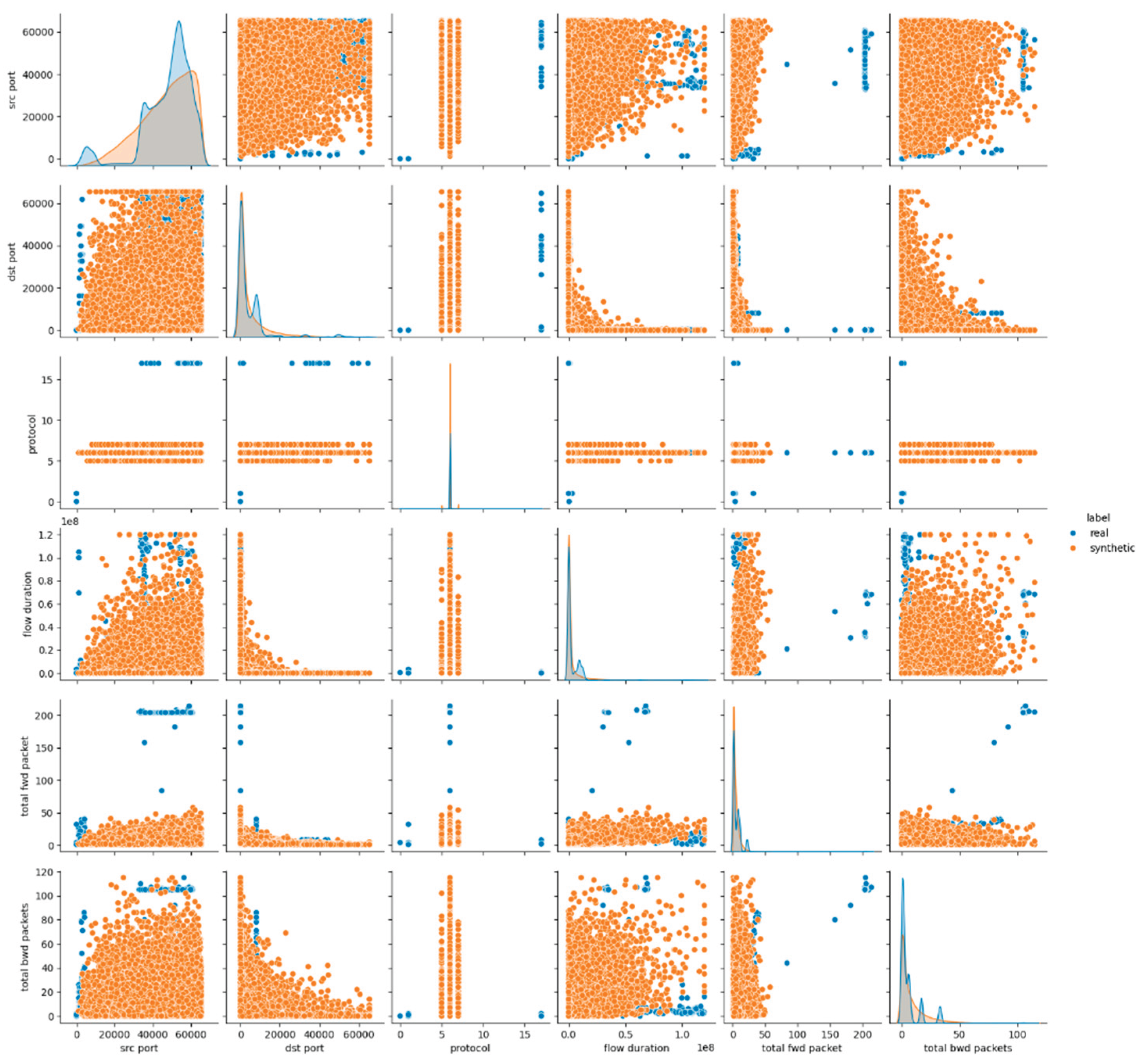
Figure 2.
Dimensionality Reduction Visualizations (using UMAP) for E1.
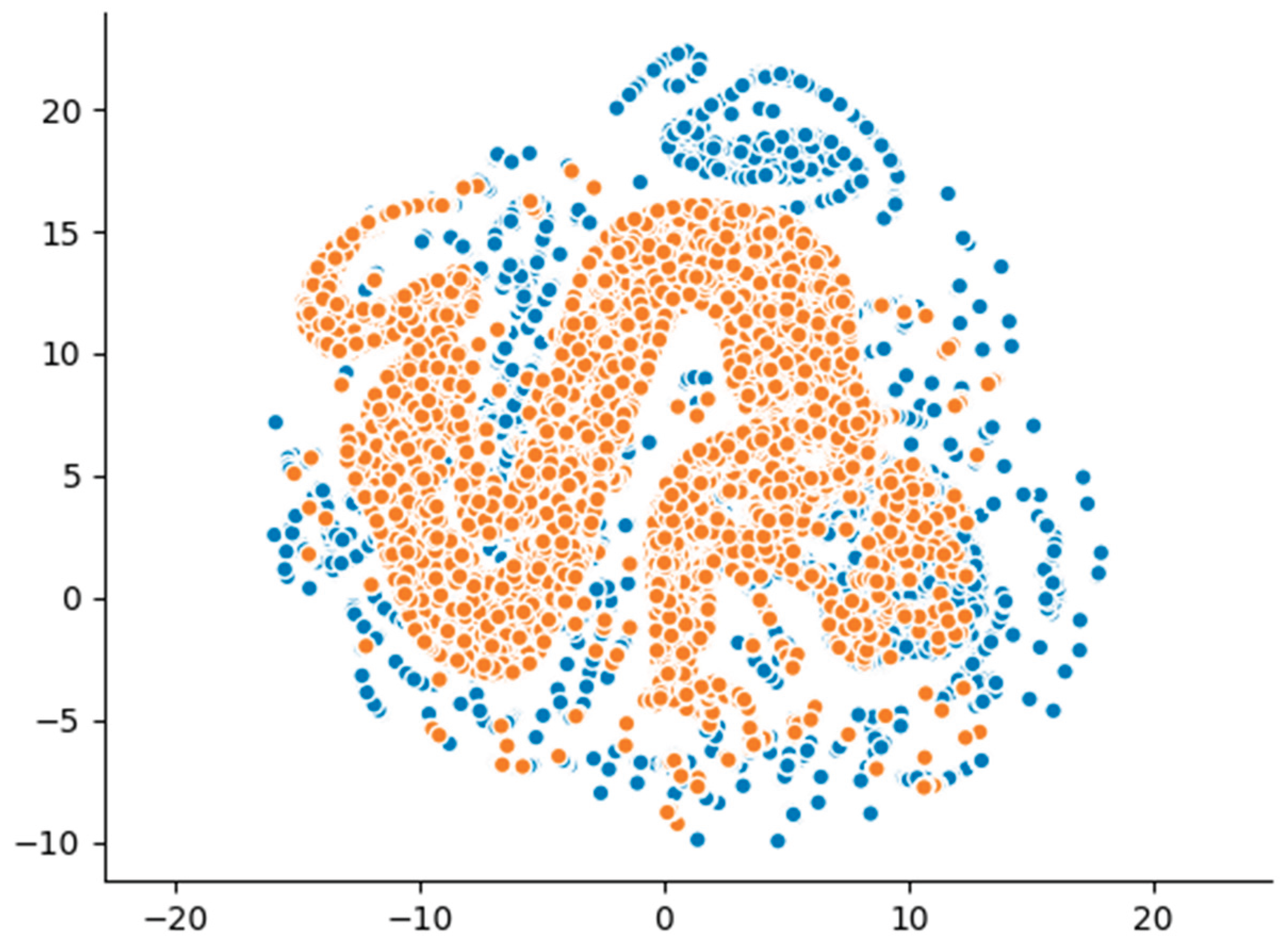
Figure 3.
Pairwise Feature Distribution Plots (Pairplots) for E2 (dataset features 1-6).
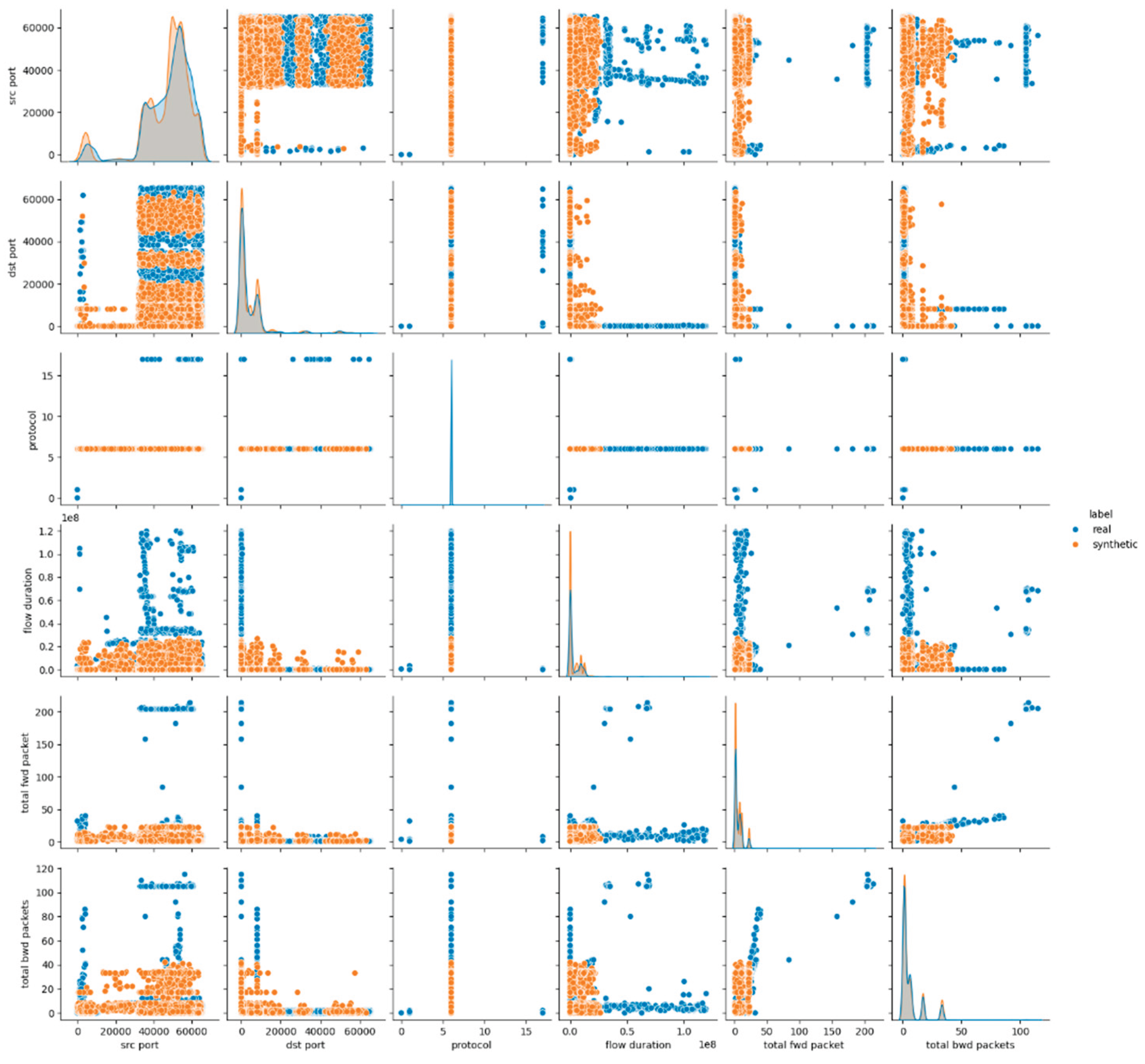
Figure 4.
Dimensionality Reduction Visualizations (using UMAP) for E2.
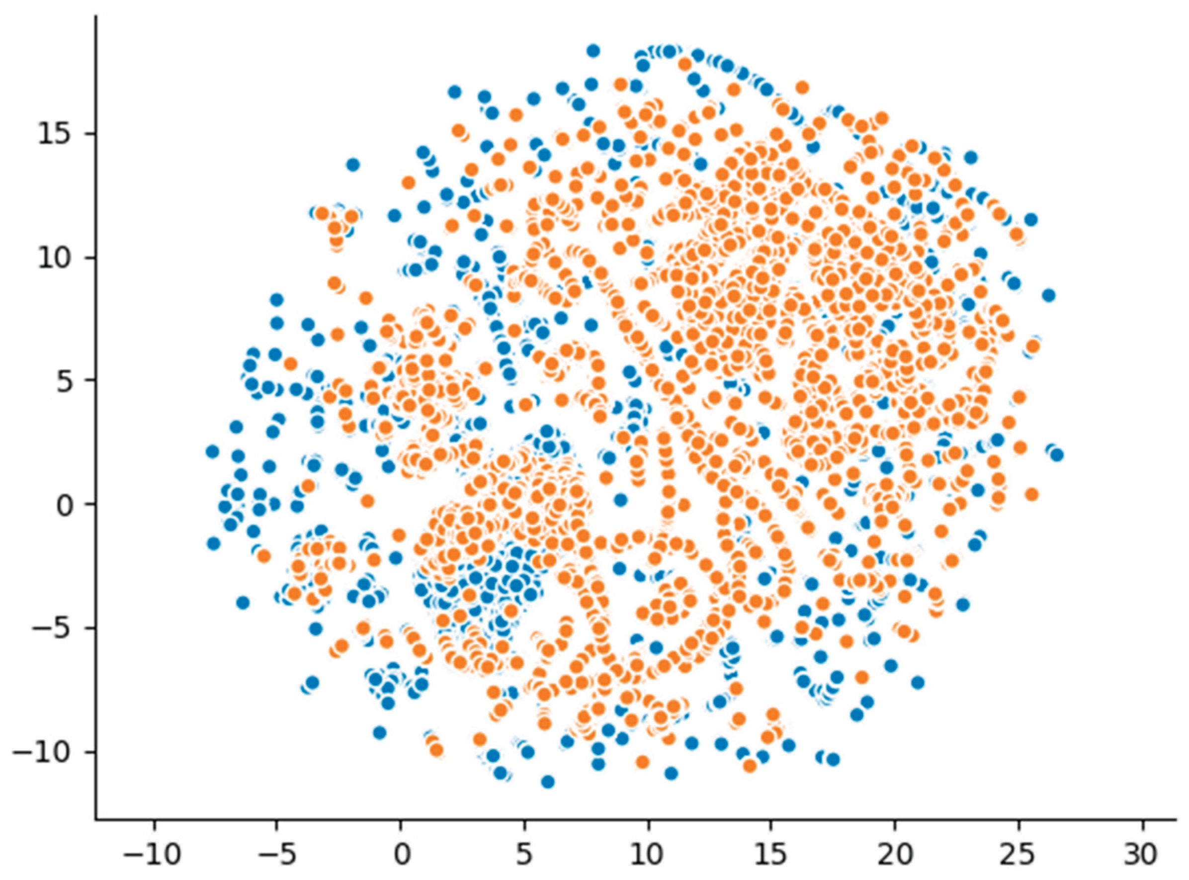
Figure 5.
Pairwise Feature Distribution Plots (Pairplots) for E3 (dataset features 1-6).
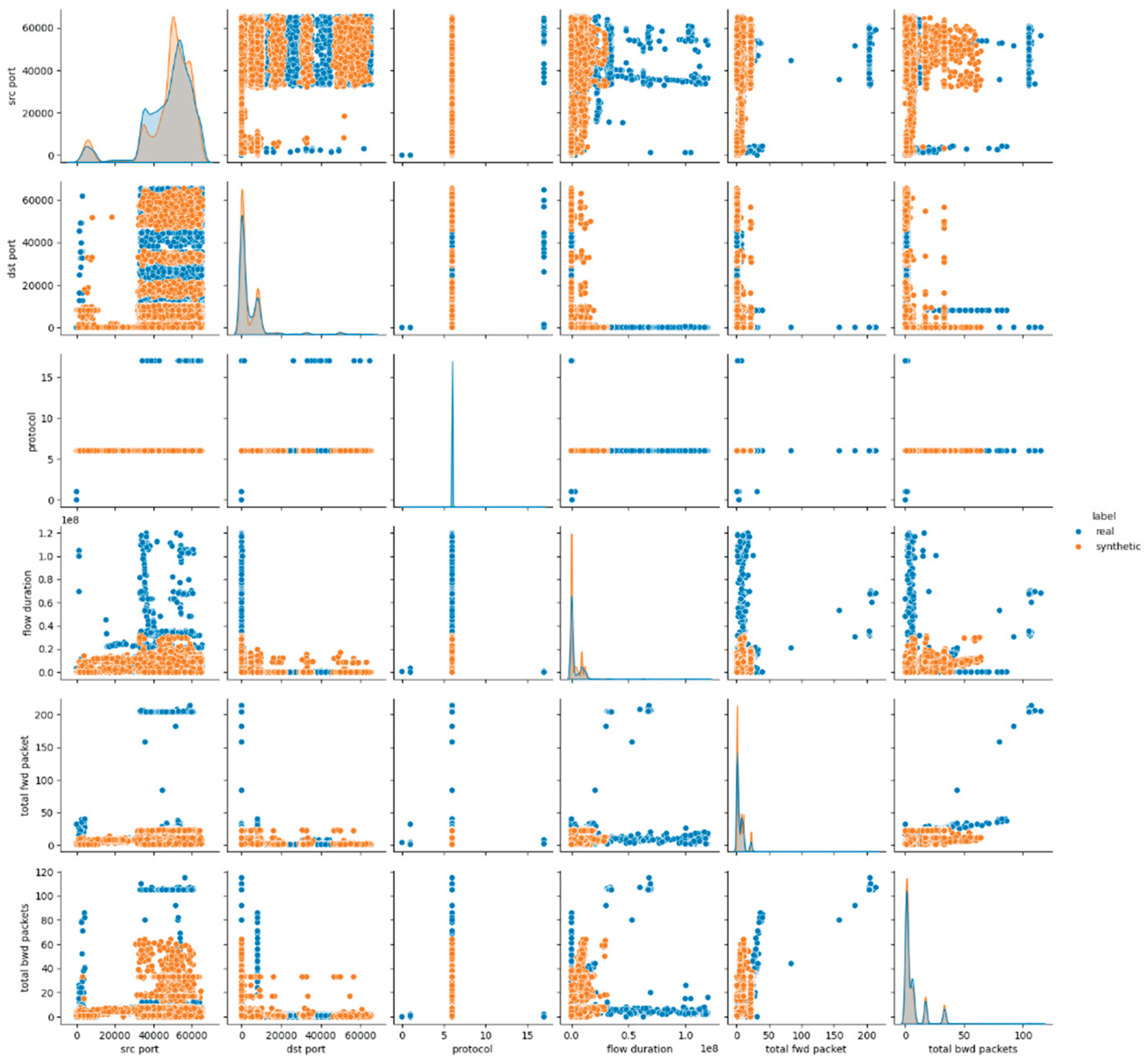
Figure 6.
Dimensionality Reduction Visualizations (using UMAP) for E3.
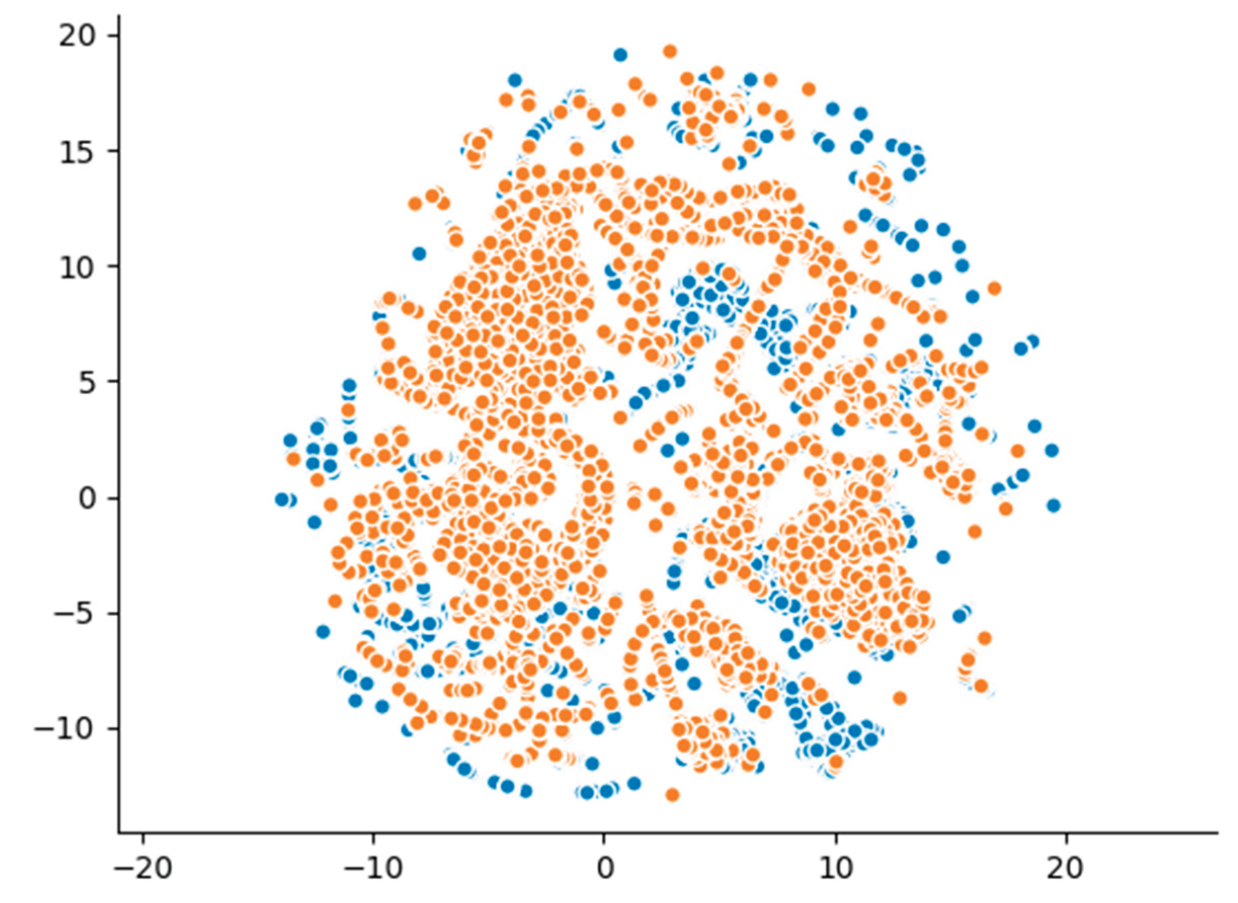
Figure 7.
Pairwise Feature Distribution Plots (Pairplots) for E4 (dataset features 1-6).
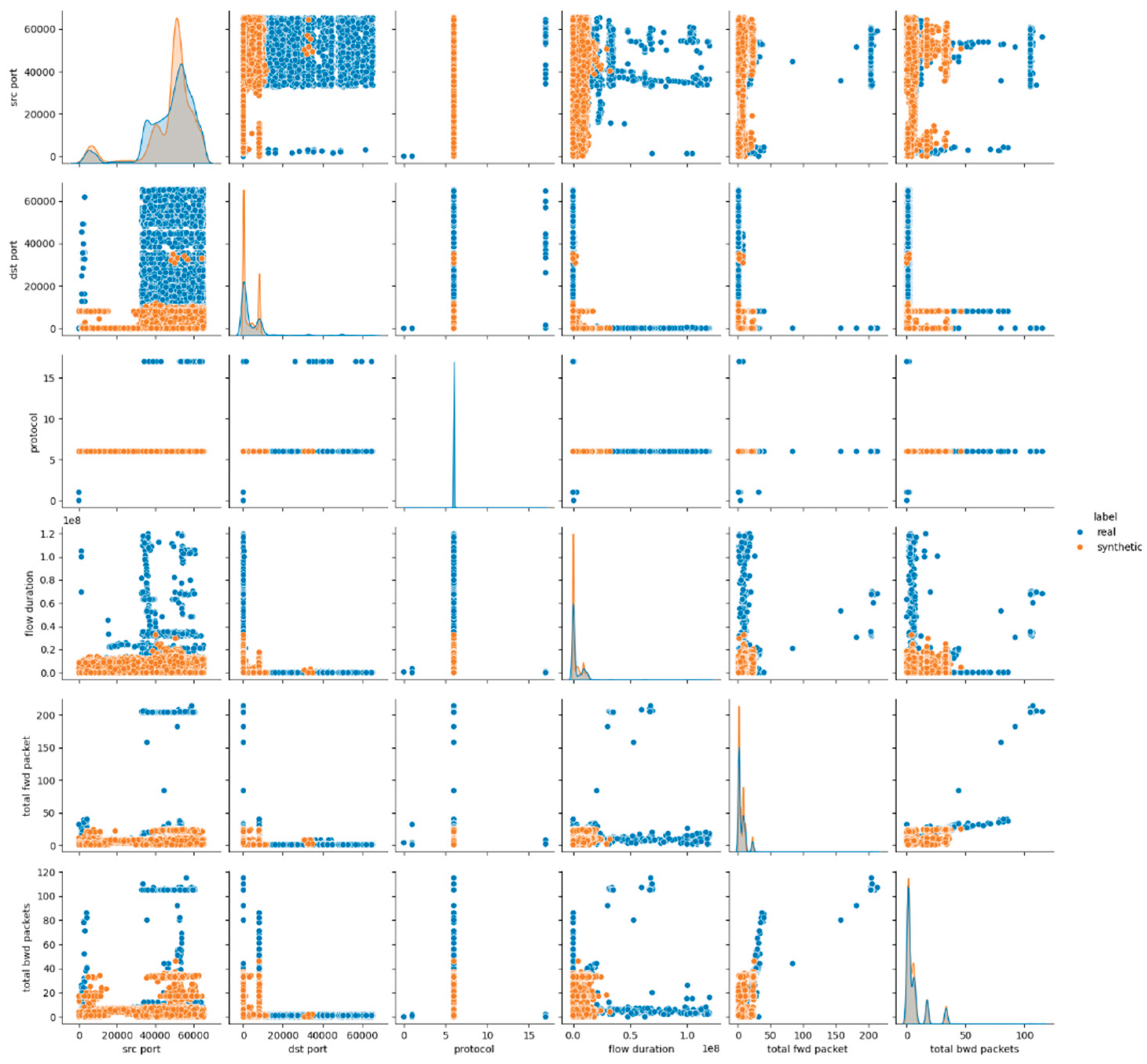
Figure 8.
Dimensionality Reduction Visualizations (using UMAP) for E4.
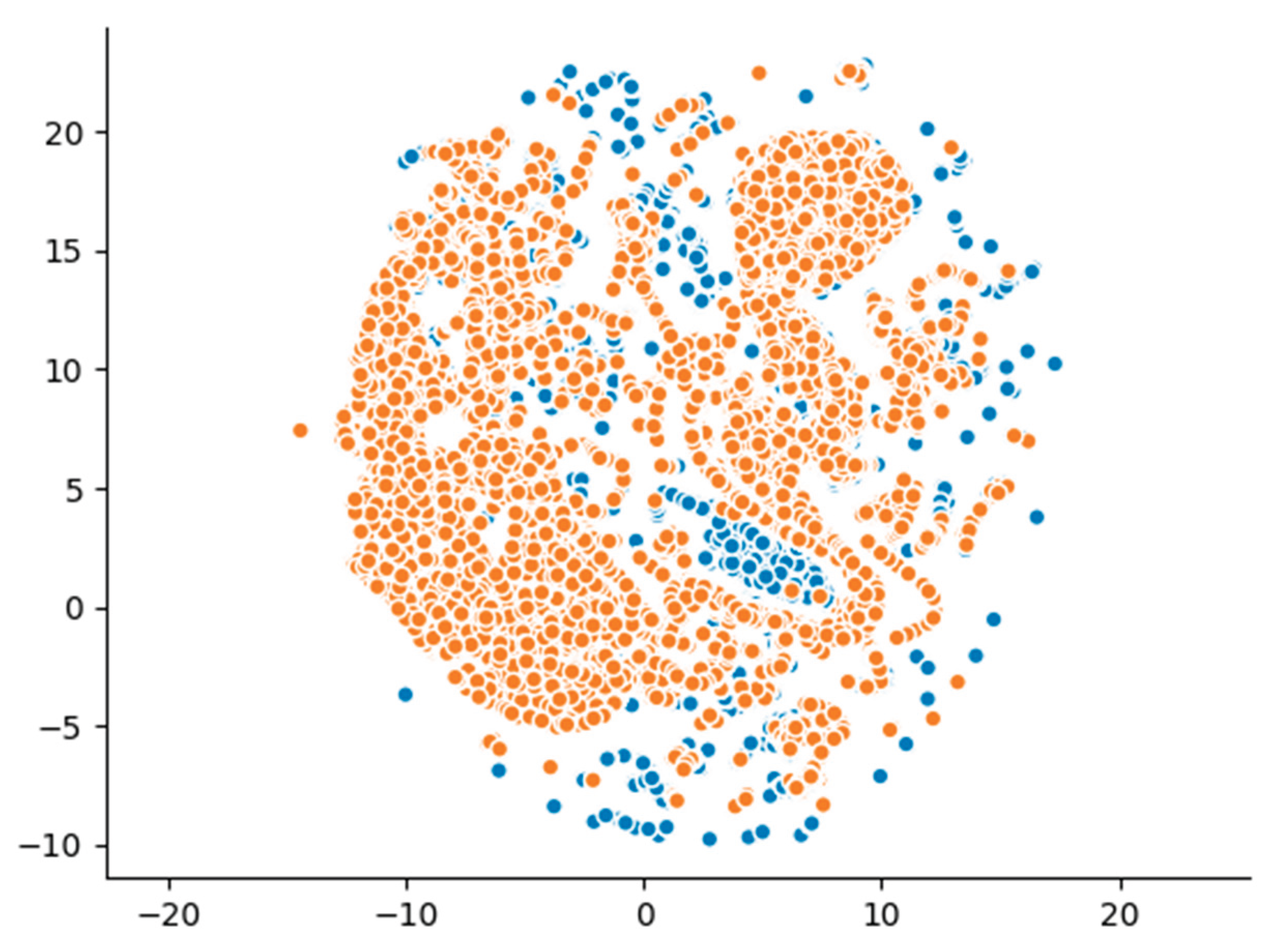
Figure 9.
Pairwise Feature Distribution Plots (Pairplots) for E5 (dataset features 1-6).

Figure 10.
Dimensionality Reduction Visualizations (using UMAP) for E5.
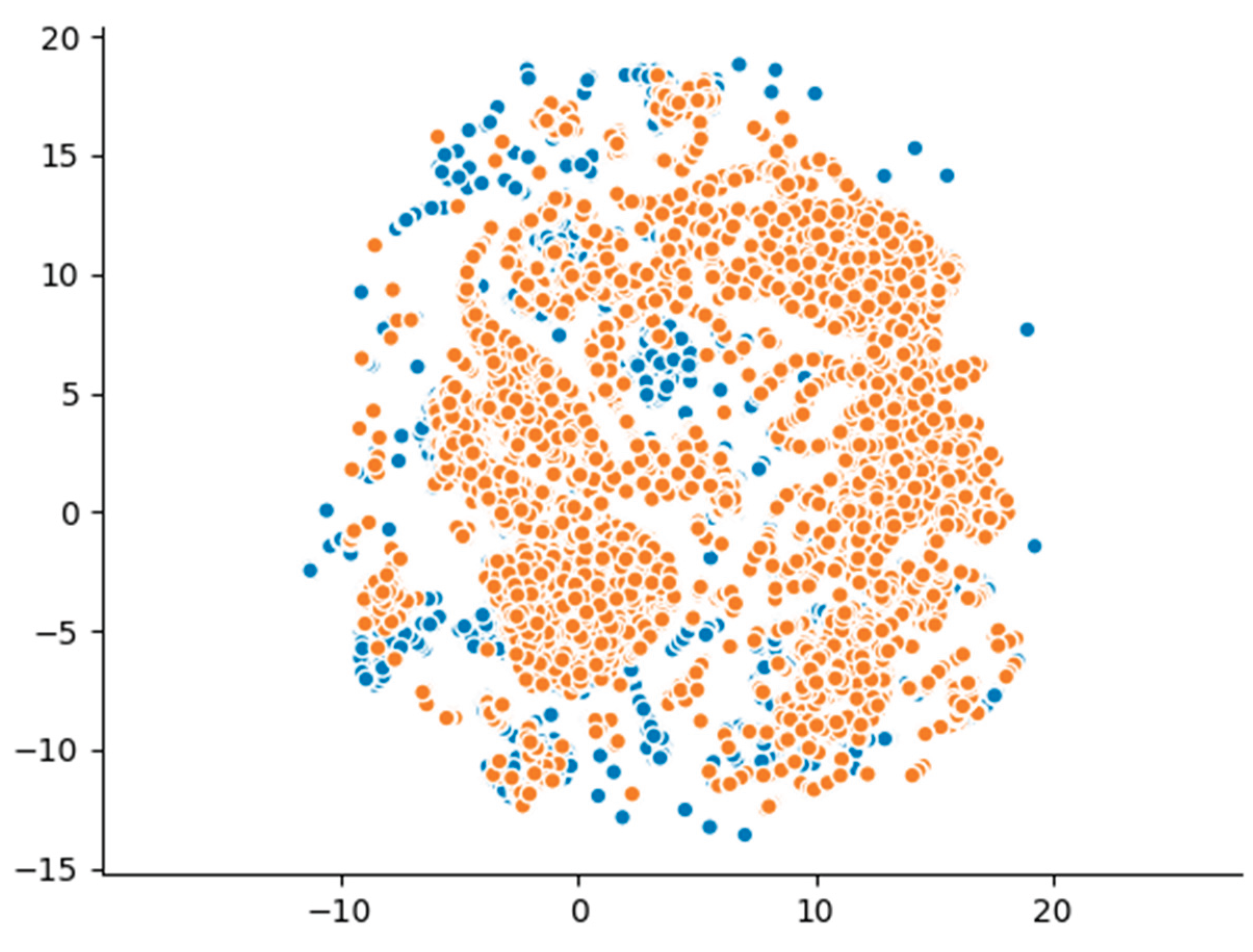
Figure 11.
Pairwise Feature Distribution Plots (Pairplots) for E6 (dataset features 1-6).
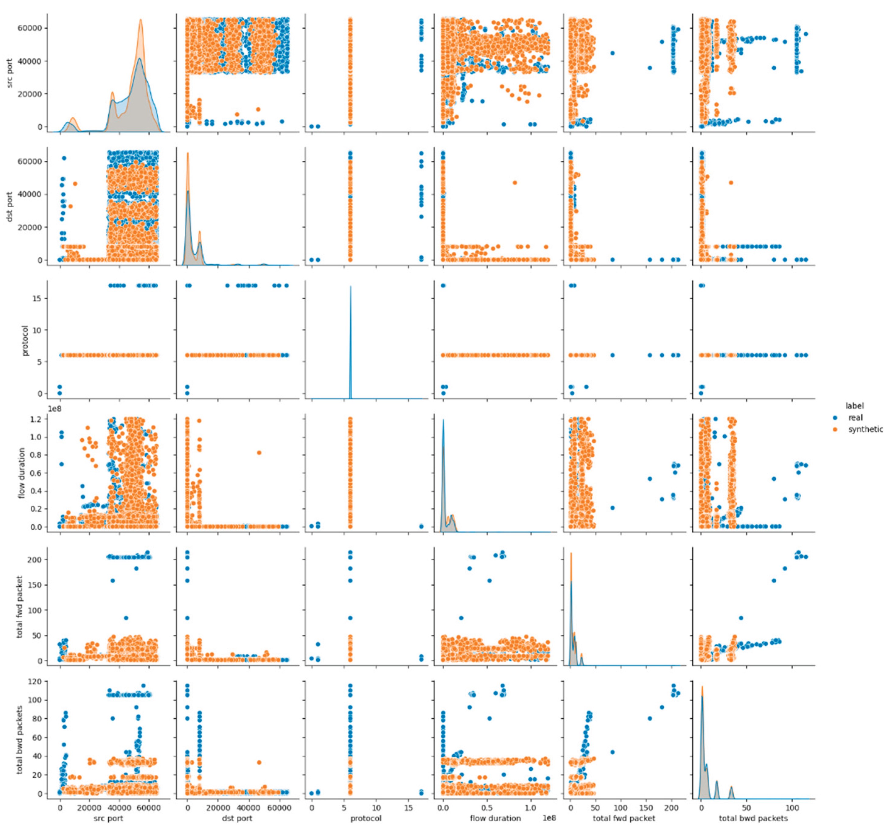
Figure 12.
Dimensionality Reduction Visualizations (using UMAP) for E6.

Figure 13.
Pairwise Feature Distribution Plots (Pairplots) for E7 (dataset features 1-6).
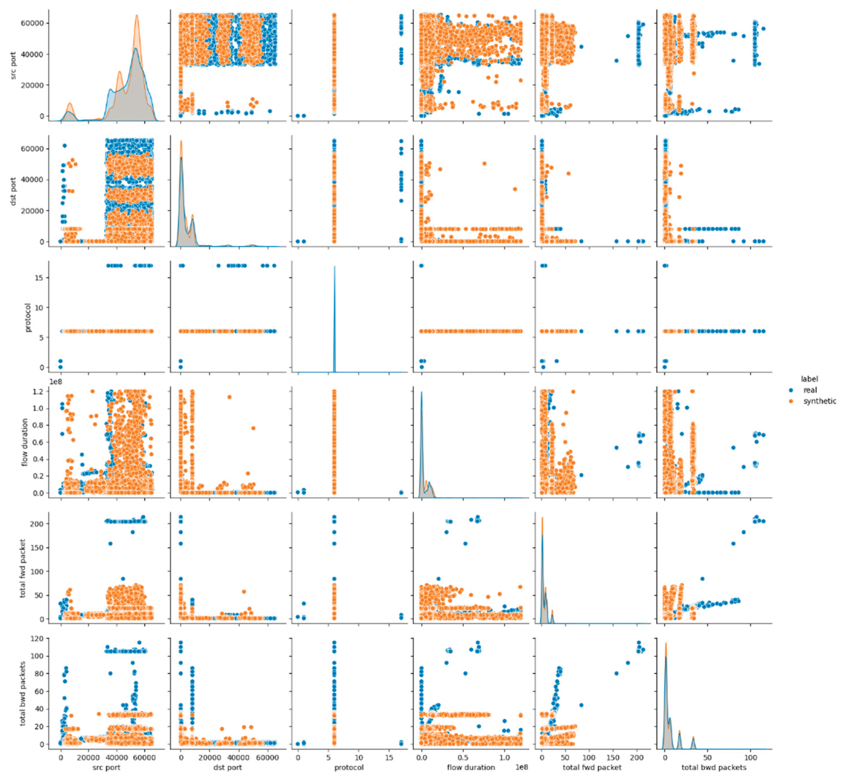
Figure 14.
Dimensionality Reduction Visualizations (using UMAP) for E7.
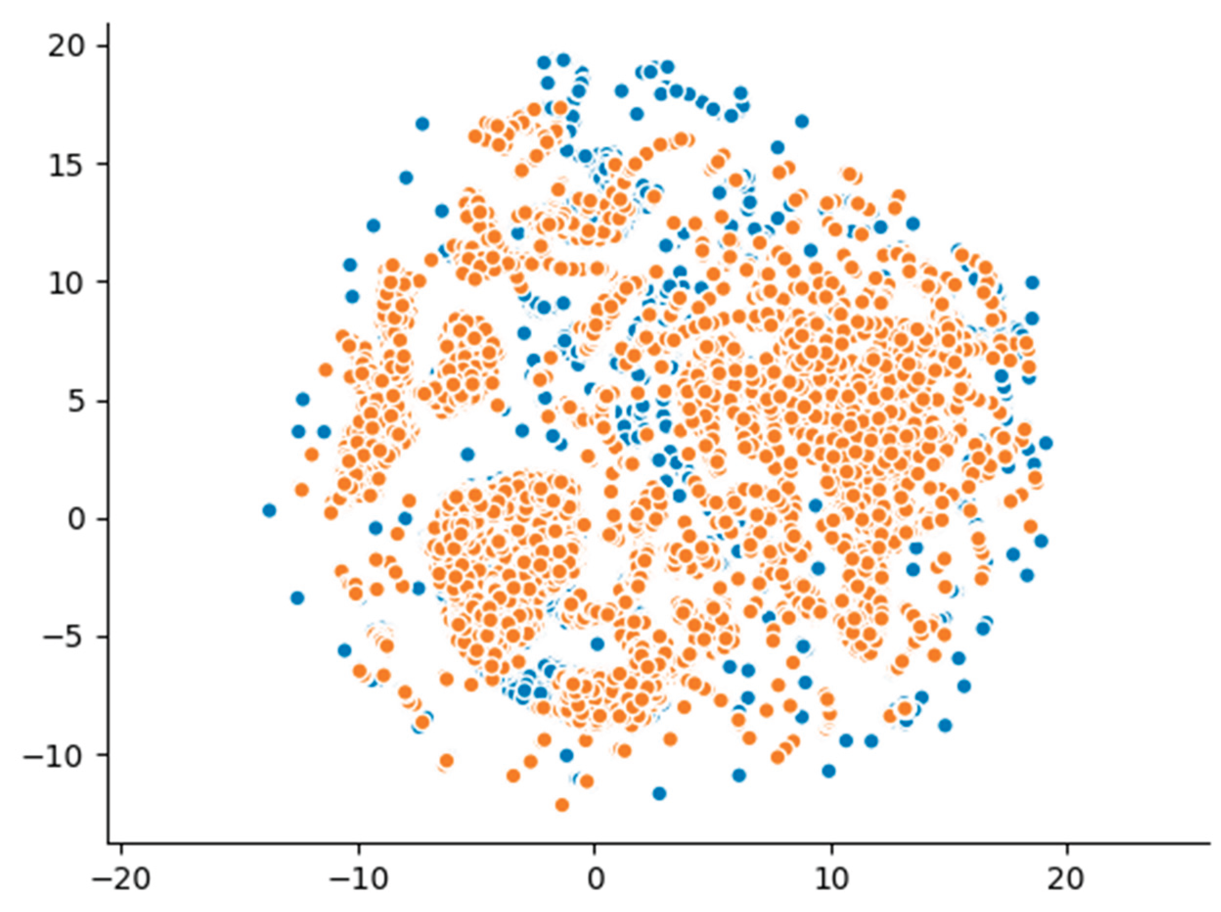

Table 1.
Key feature types included in the preprocessed, final dataset.
| Feature Type | Type | Description |
|---|---|---|
| src port | Numerical | Source port number |
| dst port | Numerical | Destination port number |
| protocol | Categorical | Protocol identifier |
| flow duration | Numerical | Duration of the flow session |
| total fwd packet | Numerical | Total number of packets in forward direction |
| total bwd packets | Numerical | Total number of packets in backward direction |
| total length of fwd packet | Numerical | Total length of forward packets |
| total length of bwd packet | Numerical | Total length of backward packets |
| flow bytes/s | Numerical | Data transfer rate in bytes per second |
| flow packets/s | Numerical | Packet transfer rate per second |
| fwd header length | Numerical | Header length in forward direction |
| bwd header length | Numerical | Header length in backward direction |
| fwd packets/s | Numerical | Forward packet transfer rate |
| bwd packets/s | Numerical | Backward packet transfer rate |
| down/up ratio | Numerical | Download to upload ratio |
| icmp code | Numerical | ICMP code |
| icmp type | Numerical | ICMP type |
| total tcp flow time | Numerical | Total duration of TCP flow |
| label | Categorical | Attack category label |
Table 2.
Key configuration parameters for each synthesizer.
| Synthesizer | Model Type | Tunable Parameters |
|---|---|---|
| GaussianCopula Synthesizer | Statistical | - |
| CTGAN Synthesizer | Deep Gan | Batch Size, Epochs, Embedding Dimension, Discriminator Dimension |
| TVAE Synthesizer | Deep VAE | Batch Size, Epochs, Embedding Dimension, Decompress Dimension |
| CopulaGAN Synthesizer | Hybrid | Batch Size, Epochs, Embedding Dimension, Discriminator Dimension |
Table 3.
Hyperparameter Variation Summary.
| Parameter | Tested Values | Description |
|---|---|---|
| Epochs | 100, 300 | Number of full passes over the training dataset - higher values allow longer learning but may increase overfitting risk |
| Batch Size | 500, 1000 | Number of samples processed per training iteration - affects convergence speed and stability |
| Network Dimensions | (128,128), (256,256) | Number of neurons in each hidden layer of the generator, discriminator, encoder, or decoder; higher dimensions enable learning of more complex patterns |
| Decompress Dimension | (128,128), (256,256) | Specifies the size of the latent vector output by the decoder when reconstructing synthetic samples from the latent space. |
| Embedding Dimension | 128, 256 | Defines the size of the latent vector used by the generator or encoder to represent compressed data features during training. |
| Model Type - Statistical | Gaussian Copula | Baseline statistical model - no variation applied |
| Model Type – DL | CTGAN, TVAE, CopulaGAN |
Deep generative models - all tested under varied configurations |
Table 4.
Evaluation metrics categorized by the primary assessment objective.
| Category | Metric | Description |
|---|---|---|
| Sample Level Metrics | Random Forest Classifier | Binary classifier trained to distinguish real from synthetic samples - realistic synthetic data should make classification accuracy approach random guessing (≈ 50%) |
| Dataset Level Metrics | Kolmogorov-Smirnov Two-Sample (Ks_2amp) Test | Statistical test that compares the cumulative distributions of real and synthetic datasets to assess their overall similarity at the dataset level |
| Detection Metrics | Logistic Detection | Uses a logistic regression model to distinguish real from synthetic data; a lower detection score (closer to random guessing) indicates higher synthetic data quality |
| SVC Detection | Applies a Support Vector Classifier to detect synthetic data; high confusion between real and synthetic samples suggests better data realism. | |
| Utility (TSTR Framework) Metrics | Random Forest Regressor | Evaluates whether patterns learned from synthetic data can generalize to real data by training a regression model on synthetic samples and testing it on real data (TSTR) - performance close to real-to-real training suggests high utility |
| Statistical Metrics | Kolmogorov-Smirnov (KS) Test | Evaluates whether the univariate distributions of continuous features in the synthetic data match those of the real data - detects distributional shifts or mode collapse |
| SDV Diagnostic Metrics | Built-In SDV Diagnostic Test | Performs automated checks on synthetic data validity, such as uniqueness of primary keys, adherence to real data ranges and categorical value consistency |
| Buit-In SDV Data Quality/Statistical Similarity Test | Provides an overall statistical similarity score between real and synthetic datasets, expressed as a percentage (0–100%), reflecting how closely the synthetic data matches the real data's statistical properties | |
| Column Shapes Sub-scores | Reports feature-wise similarity scores, indicating which columns have distributions that closely match the real data and highlight those with the highest and lowest fidelity | |
| Visual Metrics | Pairplots | Visualize bivariate distributions of features to compare relationships and spot discrepancies between real and synthetic data |
| Umap | Dimensionality reduction technique used to visually assess structural similarity between real and synthetic datasets; overlapping clusters suggest high fidelity |
Table 5.
Summary of the variation experiments.
| Experiment ID | Synthesizer | Epoch | Batch Size | Embedding Dimension | Network Dimension |
|---|---|---|---|---|---|
| E1 | GC | - | - | - | |
| Ε2 | CTGAN | 100 | 500 | 128 | (128,128) |
| Ε3 | CTGAN | 300 | 1000 | 256 | (256,256) |
| Ε4 | TVAE | 100 | 500 | 128 | (128,128) |
| Ε5 | TVAE | 300 | 1000 | 256 | (256,256) |
| Ε6 | CGAN | 100 | 500 | 128 | (128,128) |
| E7 | CGAN | 300 | 1000 | 256 | (256,256) |
Table 6.
Summary of the variation experiments.
| Attack Type | Total Records |
|---|---|
| Infiltration | 10,000 |
| Dos | 10,000 |
| Portscan | 10,000 |
| Brute-Force | 6,972 |
| Bot | 4,803 |
| Web Attack | 1,401 |
Table 7.
Evaluation Results for Gaussian Copula Model (E1).
| Category | Metric | Description |
|---|---|---|
| Sample Level Metrics | Random Forest Classifier | Classification Accuracy: 0.999 |
| Dataset Level Metrics | Kolmogorov-Smirnov Two-Sample (Ks_2amp) Test | src port: 0.0000 (Significantly different), dst port: 0.0000 (Significantly different), protocol: 0.0000 (Not significantly different), flow duration: 0.0000 (Significantly different), total fwd packet: 0.0000 (Significantly different), total bwd packets: 0.0000 (Significantly different), total length of fwd packet: 0.0000 (Significantly different), total length of bwd packet: 0.0000 (Significantly different), flow bytes/s: 0.0000 (Significantly different), flow packets/s: 0.0000 (Significantly different), fwd header length: 0.0000 (Significantly different), bwd header length: 0.0000 (Significantly different), fwd packets/s: 0.0000 (Significantly different), bwd packets/s: 0.0000 (Significantly different), down/up ratio: 0.0000 (Significantly different), icmp code: 1.0000 (Not significantly different), icmp type: 1.0000 (Not significantly different), total tcp flow time: 0.0000 (Significantly different) |
| Detection Metrics | Logistic Detection | Score: 0.788 |
| SVC Detection | Score: 0.877 | |
| Utility (TSTR Framework) Metrics | Random Forest Regressor | TSTR Score: (0.012, -0.038) |
| Statistical Metrics | Kolmogorov-Smirnov (KS) Test | Score: 0.769 |
| SDV Diagnostic Metrics | Built-In SDV Diagnostic Test | Data Validity Score: 1.0 Data Structure Score: 1.0 Overall Score (Average): 1.0 |
| Buit-In SDV Data Quality/Statistical Similarity Test | Column Shapes Score: 0.769 Column Pair Trends Score: 0.907 Overall Score (Average): 0.839 |
|
| Column Shapes Sub-scores | src port: 0.895868, dst port: 0.771725, protocol: 0.971859, flow duration: 0.761581, total fwd packet: 0.823652, total bwd packets: 0.820965, total length of fwd packet: 0.457083, total length of bwd packet: 0.381809, flow bytes/s: 0.451408, flow packets/s: 0.859251, fwd header length: 0.726746, bwd header length: 0.758477, fwd packets/s: 0.866129, bwd packets/s: 0.800537, down/up ratio: 0.753914, icmp code: 0.999768, icmp type: 0.999768, total tcp flow time: 0.757110 |
Table 8.
Evaluation Results for CTGAN Model (E2).
| Category | Metric | Description |
|---|---|---|
| Sample Level Metrics | Random Forest Classifier | Classification Accuracy: 0.999 |
| Dataset Level Metrics | Kolmogorov-Smirnov Two-Sample (Ks_2amp) Test | src port: 0.0000 (Significantly different), dst port: 0.0000 (Significantly different), protocol: 1.0000 (Not significantly different), flow duration: 0.0000 (Significantly different), total fwd packet: 0.0000 (Significantly different), total bwd packets: 0.0000 (Significantly different), total length of fwd packet: 0.0000 (Significantly different), total length of bwd packet: 0.0000 (Significantly different), flow bytes/s: 0.0000 (Significantly different), flow packets/s: 0.0000 (Significantly different), fwd header length: 0.0000 (Significantly different), bwd header length: 0.0000 (Significantly different), fwd packets/s: 0.0000 (Significantly different), bwd packets/s: 0.0000 (Significantly different), down/up ratio: 0.0000 (Significantly different), icmp code: 1.0000 (Not significantly different), icmp type: 1.0000 (Not significantly different), total tcp flow time: 0.0000 (Significantly different) |
| Detection Metrics | Logistic Detection | Score: 0.788 |
| SVC Detection | Score: 0.877 | |
| Utility (TSTR Framework) Metrics | Random Forest Regressor | TSTR Score: (-0.035, -0.002) |
| Statistical Metrics | Kolmogorov-Smirnov (KS) Test | Score: 0.811 |
| SDV Diagnostic Metrics | Built-In SDV Diagnostic Test | Data Validity Score: 1.0 Data Structure Score: 1.0 Overall Score (Average): 1.0 |
| Buit-In SDV Data Quality/Statistical Similarity Test | Column Shapes Score: 0.809 Column Pair Trends Score: 0.932 Overall Score (Average): 0.871 |
|
| Column Shapes Sub-scores | src port: 0.924935, dst port: 0.745391, protocol: 0.999189, flow duration: 0.686238, total fwd packet: 0.940615, total bwd packets: 0.946359, total length of fwd packet: 0.885538, total length of bwd packet: 0.770196, flow bytes/s: 0.496317, flow packets/s: 0.698606, fwd header length: 0.850982, bwd header length: 0.797943, fwd packets/s: 0.754910, bwd packets/s: 0.697517, down/up ratio: 0.727603, icmp code: 0.999768, icmp type: 0.999768, total tcp flow time: 0.656105 |
Table 9.
Evaluation Results for CTGAN Model (E3).
| Category | Metric | Description |
|---|---|---|
| Sample Level Metrics | Random Forest Classifier | Classification Accuracy: 1.0 |
| Dataset Level Metrics | Kolmogorov-Smirnov Two-Sample (Ks_2amp) Test | src port: 0.0000 (Significantly different), dst port: 0.0000 (Significantly different), protocol: 1.0000 (Not significantly different), flow duration: 0.0000 (Significantly different), total fwd packet: 0.0000 (Significantly different), total bwd packets: 0.0000 (Significantly different), total length of fwd packet: 0.0000 (Significantly different), total length of bwd packet: 0.0000 (Significantly different), flow bytes/s: 0.0000 (Significantly different), flow packets/s: 0.0000 (Significantly different), fwd header length: 0.0000 (Significantly different), bwd header length: 0.0000 (Significantly different), fwd packets/s: 0.0000 (Significantly different), bwd packets/s: 0.0000 (Significantly different), down/up ratio: 0.0000 (Significantly different), icmp code: 1.0000 (Not significantly different), icmp type: 1.0000 (Not significantly different), total tcp flow time: 0.0000 (Significantly different) |
| Detection Metrics | Logistic Detection | Score: 0.806 |
| SVC Detection | Score: 0.753 | |
| Utility (TSTR Framework) Metrics | Random Forest Regressor | TSTR Score: (0.072, -0.003) |
| Statistical Metrics | Kolmogorov-Smirnov (KS) Test | Score: 0.797 |
| SDV Diagnostic Metrics | Built-In SDV Diagnostic Test | Data Validity Score: 1.0 Data Structure Score: 1.0 Overall Score (Average): 1.0 |
| Buit-In SDV Data Quality/Statistical Similarity Test | Column Shapes Score: 0.797 Column Pair Trends Score: 0.929 Overall Score (Average): 0.863 |
|
| Column Shapes Sub-scores | src port: 0.910066, dst port: 0.744928, protocol: 0.999189, flow duration: 0.618399, total fwd packet: 0.938438, total bwd packets: 0.950204, total length of fwd packet: 0.854734, total length of bwd packet: 0.737308, flow bytes/s: 0.462757, flow packets/s: 0.648323, fwd header length: 0.899389, bwd header length: 0.829188, fwd packets/s: 0.647976, bwd packets/s: 0.777562, down/up ratio: 0.683111, icmp code: 0.999768, icmp type: 0.999768, total tcp flow time: 0.649018 |
Table 10.
Evaluation Results for TVAE Model (E4).
| Category | Metric | Description |
|---|---|---|
| Sample Level Metrics | Random Forest Classifier | Classification Accuracy: 0.999 |
| Dataset Level Metrics | Kolmogorov-Smirnov Two-Sample (Ks_2amp) Test | src port: 0.0000 (Significantly different), dst port: 0.0000 (Significantly different), protocol: 1.0000 (Not significantly different), flow duration: 0.0000 (Significantly different), total fwd packet: 0.0000 (Significantly different), total bwd packets: 0.0000 (Significantly different), total length of fwd packet: 0.0000 (Significantly different), total length of bwd packet: 0.0000 (Significantly different), flow bytes/s: 0.0000 (Significantly different), flow packets/s: 0.0000 (Significantly different), fwd header length: 0.0000 (Significantly different), bwd header length: 0.0000 (Significantly different), fwd packets/s: 0.0000 (Significantly different), bwd packets/s: 0.0000 (Significantly different), down/up ratio: 0.0000 (Significantly different), icmp code: 1.0000 (Not significantly different), icmp type: 1.0000 (Not significantly different), total tcp flow time: 0.0000 (Significantly different) |
| Detection Metrics | Logistic Detection | Score: 0.755 |
| SVC Detection | Score: 0.838 | |
| Utility (TSTR Framework) Metrics | Random Forest Regressor | TSTR Score: (0.918, 0.564) |
| Statistical Metrics | Kolmogorov-Smirnov (KS) Test | Score: 0.826 |
| SDV Diagnostic Metrics | Built-In SDV Diagnostic Test | Data Validity Score: 1.0 Data Structure Score: 1.0 Overall Score (Average): 1.0 |
| Buit-In SDV Data Quality/Statistical Similarity Test | Column Shapes Score: 0.826 Column Pair Trends Score: 0.925 Overall Score (Average): 0.876 |
|
| Column Shapes Sub-scores | src port: 0.902677, dst port: 0.774134, protocol: 0.999189, flow duration: 0.734528, total fwd packet: 0.909325, total bwd packets: 0.928062, total length of fwd packet: 0.764128, total length of bwd packet: 0.741824, flow bytes/s: 0.786316, flow packets/s: 0.701177, fwd header length: 0.852163, bwd header length: 0.806189, fwd packets/s: 0.728877, bwd packets/s: 0.841393, down/up ratio: 0.726214, icmp code: 0.999768, icmp type: 0.999768, total tcp flow time: 0.667315 |
Table 11.
Evaluation Results for TVAE Model (E5).
| Category | Metric | Description |
|---|---|---|
| Sample Level Metrics | Random Forest Classifier | Classification Accuracy: 0.999 |
| Dataset Level Metrics | Kolmogorov-Smirnov Two-Sample (Ks_2amp) Test | src port: 0.0000 (Significantly different), dst port: 0.0000 (Significantly different), protocol: 1.0000 (Not significantly different), flow duration: 0.0000 (Significantly different), total fwd packet: 0.0000 (Significantly different), total bwd packets: 0.0000 (Significantly different), total length of fwd packet: 0.0000 (Significantly different), total length of bwd packet: 0.0000 (Significantly different), flow bytes/s: 0.0000 (Significantly different), flow packets/s: 0.0000 (Significantly different), fwd header length: 0.0000 (Significantly different), bwd header length: 0.0000 (Significantly different), fwd packets/s: 0.0000 (Significantly different), bwd packets/s: 0.0000 (Significantly different), down/up ratio: 0.0000 (Significantly different), icmp code: 1.0000 (Not significantly different), icmp type: 1.0000 (Not significantly different), total tcp flow time: 0.0000 (Significantly different) |
| Detection Metrics | Logistic Detection | Score: 0.708 |
| SVC Detection | Score: 0.841 | |
| Utility (TSTR Framework) Metrics | Random Forest Regressor | TSTR Score: (0.918, 0.564) |
| Statistical Metrics | Kolmogorov-Smirnov (KS) Test | Score: 0.849 |
| SDV Diagnostic Metrics | Built-In SDV Diagnostic Test | Data Validity Score: 1.0 Data Structure Score: 1.0 Overall Score (Average): 1.0 |
| Buit-In SDV Data Quality/Statistical Similarity Test | Column Shapes Score: 0.85 Column Pair Trends Score: 0.9234 Overall Score (Average): 0.8922 |
|
| Column Shapes Sub-scores | src port: 0.876390, dst port: 0.778025, protocol: 0.999189, flow duration: 0.733046, total fwd packet: 0.940986, total bwd packets: 0.957083, total length of fwd packet: 0.837711, total length of bwd packet: 0.772698, flow bytes/s: 0.771378, flow packets/s: 0.786386, fwd header length: 0.896262, bwd header length: 0.881161, fwd packets/s: 0.811145, bwd packets/s: 0.844659, down/up ratio: 0.724917, icmp code: 0.999768, icmp type: 0.999768, total tcp flow time: 0.689040 |
Table 12.
Evaluation Results for CopulaGAN Model (E6).
| Category | Metric | Description |
|---|---|---|
| Sample Level Metrics | Random Forest Classifier | Classification Accuracy: 0.999 |
| Dataset Level Metrics | Kolmogorov-Smirnov Two-Sample (Ks_2amp) Test | src port: 0.0000 (Significantly different), dst port: 0.0000 (Significantly different), protocol: 1.0000 (Not significantly different), flow duration: 0.0000 (Significantly different), total fwd packet: 0.0000 (Significantly different), total bwd packets: 0.0000 (Significantly different), total length of fwd packet: 0.0000 (Significantly different), total length of bwd packet: 0.0000 (Significantly different), flow bytes/s: 0.0000 (Significantly different), flow packets/s: 0.0000 (Significantly different), fwd header length: 0.0000 (Significantly different), bwd header length: 0.0000 (Significantly different), fwd packets/s: 0.0000 (Significantly different), bwd packets/s: 0.0000 (Significantly different), down/up ratio: 0.0000 (Significantly different), icmp code: 1.0000 (Not significantly different), icmp type: 1.0000 (Not significantly different), total tcp flow time: 0.0000 (Significantly different) |
| Detection Metrics | Logistic Detection | Score: 0.788 |
| SVC Detection | Score: 0.877 | |
| Utility (TSTR Framework) Metrics | Random Forest Regressor | TSTR Score: (0.178, -0074.) |
| Statistical Metrics | Kolmogorov-Smirnov (KS) Test | Score: 0.893 |
| SDV Diagnostic Metrics | Built-In SDV Diagnostic Test | Data Validity Score: 1.0 Data Structure Score: 1.0 Overall Score (Average): 1.0 |
| Buit-In SDV Data Quality/Statistical Similarity Test | Column Shapes Score: 0.893 Column Pair Trends Score: 0.951 Overall Score (Average): 0.922 |
|
| Column Shapes Sub-scores | src port: 0.903233, dst port: 0.739740, protocol: 0.999189, flow duration: 0.877455, total fwd packet: 0.930170, total bwd packets: 0.952890, total length of fwd packet: 0.944645, total length of bwd packet: 0.878914, flow bytes/s: 0.950065, flow packets/s: 0.873911, fwd header length: 0.892510, bwd header length: 0.845910, fwd packets/s: 0.866662, bwd packets/s: 0.914559, down/up ratio: 0.628034, icmp code: 0.999768, icmp type: 0.999768, total tcp flow time: 0.872846 |
Table 13.
Evaluation Results for CopulaGAN Model (E7).
| Category | Metric | Description |
|---|---|---|
| Sample Level Metrics | Random Forest Classifier | Classification Accuracy: 0.999 |
| Dataset Level Metrics | Kolmogorov-Smirnov Two-Sample (Ks_2amp) Test | src port: 0.0000 (Significantly different), dst port: 0.0000 (Significantly different), protocol: 1.0000 (Not significantly different), flow duration: 0.0000 (Significantly different), total fwd packet: 0.0000 (Significantly different), total bwd packets: 0.0000 (Significantly different), total length of fwd packet: 0.0000 (Significantly different), total length of bwd packet: 0.0000 (Significantly different), flow bytes/s: 0.0000 (Significantly different), flow packets/s: 0.0000 (Significantly different), fwd header length: 0.0000 (Significantly different), bwd header length: 0.0000 (Significantly different), fwd packets/s: 0.0000 (Significantly different), bwd packets/s: 0.0000 (Significantly different), down/up ratio: 0.0000 (Significantly different), icmp code: 1.0000 (Not significantly different), icmp type: 1.0000 (Not significantly different), total tcp flow time: 0.0000 (Significantly different) |
| Detection Metrics | Logistic Detection | Score: 0.813 |
| SVC Detection | Score: 0.858 | |
| Utility (TSTR Framework) Metrics | Random Forest Regressor | TSTR Score: (0.075, -0045.) |
| Statistical Metrics | Kolmogorov-Smirnov (KS) Test | Score: 0.901 |
| SDV Diagnostic Metrics | Built-In SDV Diagnostic Test | Data Validity Score: 1.0 Data Structure Score: 1.0 Overall Score (Average): 1.0 |
| Buit-In SDV Data Quality/Statistical Similarity Test | Column Shapes Score: 0.903 Column Pair Trends Score: 0.958 Overall Score (Average): 0.931 |
|
| Column Shapes Sub-scores | src port: 0.928826, dst port: 0.767348, protocol: 0.999189, flow duration: 0.856402, total fwd packet: 0.934825, total bwd packets: 0.960997, total length of fwd packet: 0.944043, total length of bwd packet: 0.891120, flow bytes/s: 0.925560, flow packets/s: 0.879655, fwd header length: 0.882944, bwd header length: 0.933250, fwd packets/s: 0.833148, bwd packets/s: 0.907449, down/up ratio: 0.720516, icmp code: 0.999768, icmp type: 0.999768, total tcp flow time: 0.882435 |
Disclaimer/Publisher’s Note: The statements, opinions and data contained in all publications are solely those of the individual author(s) and contributor(s) and not of MDPI and/or the editor(s). MDPI and/or the editor(s) disclaim responsibility for any injury to people or property resulting from any ideas, methods, instructions or products referred to in the content. |
© 2025 by the authors. Licensee MDPI, Basel, Switzerland. This article is an open access article distributed under the terms and conditions of the Creative Commons Attribution (CC BY) license (http://creativecommons.org/licenses/by/4.0/).
Copyright: This open access article is published under a Creative Commons CC BY 4.0 license, which permit the free download, distribution, and reuse, provided that the author and preprint are cited in any reuse.


