
Submitted:
23 July 2025
Posted:
25 July 2025
You are already at the latest version
Abstract
In the first part of the paper we obtain the analytic solution for the profile of a shock wave in a nonlinear lossy transmission line, constructed from the inductors, the capacitors and the resistors. both the charge of a capacitor and a current through the inductor are obtained as the functions of the time and space coordinate.
In the second part of the paper we formulate the simple wave approximation for the nonlinear lossless transmission line.
Keywords:
nonlinear transmission lines
; shocks
; solitons
1. Introduction
The concept that in a nonlinear wave propagation system the various parts of the wave travel with different velocities, and that wave fronts (or tails) can sharpen into shock waves, is deeply imbedded in the classical theory of fluid dynamics [1]. The nonlinear electrical transmission lines (where the nonlinearity can be either due to nonlinear capacitors or nonlinear inductors forming the line, or both) are of much interest both due to their applications, and as the laboratories to study nonlinear waves [2]. A very interesting particular type of signals which can propagate along such lines - the shock waves - is attracting interest since long ago [3,4]. We published a series of papers on the travelling waves in nonlinear transmission lines: the kinks, the solitons and the shocks (see the most recent publication of that series and the references therein [5]).
In the present short note we would like to add to our previous publications on the subject. In the first half of the paper we start from reproducing in a concentrated form the analytic results for the profile of the shock wave in the transmission line with the nonlinear capacitors obtained in Ref. [5]. Those results were obtained by reducing the second order ordinary differential equation describing the travelling waves i the transmission line and factorising the thus obtained equation for the definite values of the parameters. While in the latter publication only the charge of the capacitors was analysed as the function of the time and the coordinate (which is equivalent to studying the voltage in the line as the function of the time and the coordinate), in the present note the time and coordinate dependence of the current is also calculated.
The second half of the paper is dedicated to the presentation of the simple wave approximation to the wave equation describing general lossless transmission line, which allows to decouple the nonlinear wave equation into two separate equations for the right- and left-going waves [6,7,8]. While we used this approximation previously for the Josephson transmission line (JTL) [9,10,11], here we formulate the approximation for the case when both the inductors and the capacitors are nonlinear [5].
2. The Circuit Equations
The transmission line constructed from the identical nonlinear inductors and the identical nonlinear capacitors is shown on Figure 1.
We take the capacitors charges and the integrated voltages on the inductors
as the dynamical variables. The circuit equations (Kirchhoff laws) are
To close the system (2) we should specify the connection between the voltages on the capacitors and the charges and also between the currents through the inductors and the integrated voltages
In the continuum approximation we treat n as the continuous variable x (we measure distance in the units of the transmission line period) and approximate the finite differences in the r.h.s. of the equations by the first derivatives with respect to x, after which the equations take the form
Further on we’ll consider the travelling waves, for which all the dependent variables depend upon the single independent variable , where U is the speed of the wave. For such waves (4) turns into the system of ODE which after integration takes the form
where and are the constants of integration.
Equation (5) contains 3 arbitrary constants - U, and . Since we are considering localized travelling waves, it would be convenient to take as the constants , defined by the equations
and connected by the relation
Thus Equation (5) can be presented as
where and .
The speed of the travelling wave is
3. Half-Nonlinear Transmission Line
Further on we consider transmission line with the linear inductors (). and nonlinear capacitors. We can exclude the current from (8) and after a bit of algebra obtain closed equation for
and the travelling speed is given by the equation
The solution of (10) should satisfy the boundary conditions (6a).
4. The ODE Which Doesn’t Contain Explicitly the Independent Variable
Following the well known in mathematics principle, stating that the more general the problem is, the easier it is to solve it, let us change gears and instead of (13) and (17) consider the generalized damped Helmholtz-Duffing equation [11]
where n, k, , , are constants, with the boundary conditions
Equation (19) doesn’t contain explicitly the independent variable . This prompts the idea to consider x as the new independent variable and
as the new dependent variable. In the new variables (19) takes the form of Abel equation of the second kind [12].
The boundary conditions in the new variables are
One can easily check up that for and k connected by the formula
the solution of (22) satisfying the boundary conditions (23) is
Substituting into (21) and integrating we obtain the solution of (19) as
Now consider the equation
with the boundary conditions (20). We can present (27) as
Hence we realize that for k and connected by the formula
the solution of (27) satisfying the boundary conditions (23) is
Let us return to (19) and modify it to
Thus we take into account possible nonlinearity of friction. Thus instead of (22) we obtain
Acting as above we obtain that for k and connected by the formula
the solution of (32) satisfying the boundary conditions (23) is (25) (same as it was for ), only this time
Hence the solution of (31) with is of the same form as for (Equation (26)), only with the modified m.
5. Back to the Transmission Line
Now let us return to the transmission line. For Equation (13) with given by (17), using the results of the previous Section, we claim that when the parameters of the equation satisfy the relation
the solution of the equation can be expressed in terms of elementary functions:
where
For (13) with given by (15), we claim that when the boundary conditions satisfy the relation
the solution of the equation can be expressed in terms of elementary functions:
where
Note that (36) doesn’t goes to (39) when . More specifically, when , the solution (36) goes to the weak shock solution. On the other hand, the solution (39) corresponds to the case when both terms in (13) are of the same order of magnitude.
We used previously the linear approximation for in the last term in the l.h.s. of (10). Strictly speaking, since we are considering nonlinear in the r.h.s. of (10) more consistent would be to treat the same way the l.h.s. Equations. (33), (34) allow us to go one step in this direction, that is to consider in the last term in the l.h.s. of (10) in quadratic approximation (for cubic nonlinearity of ). As the result, Equations (35) and (36) slightly change and Equation (36) doesn’t change at all.
The analytic results for the profile of the shock wave were obtained by reducing the second order differential Equation (10) to the first order one
where . However, looking back to Equation (8) we see the opportunity to reduce the system of two first order differential equations to the single first order one
already at this stage. It would be interesting to try to obtain exact analytic solutions of (42) for some values of the parameters.
Postponing such attempt until later time, note here that Equation (42) allows us to obtain the dependence of the current I which was absent in our previous publications. To achieve this aim let us rewrite (42) in the form
The dependence being found earlier, Equation (43) gives infinite series for , and the first two terms of the series are
Thus from (36) follows
and from (39) follows
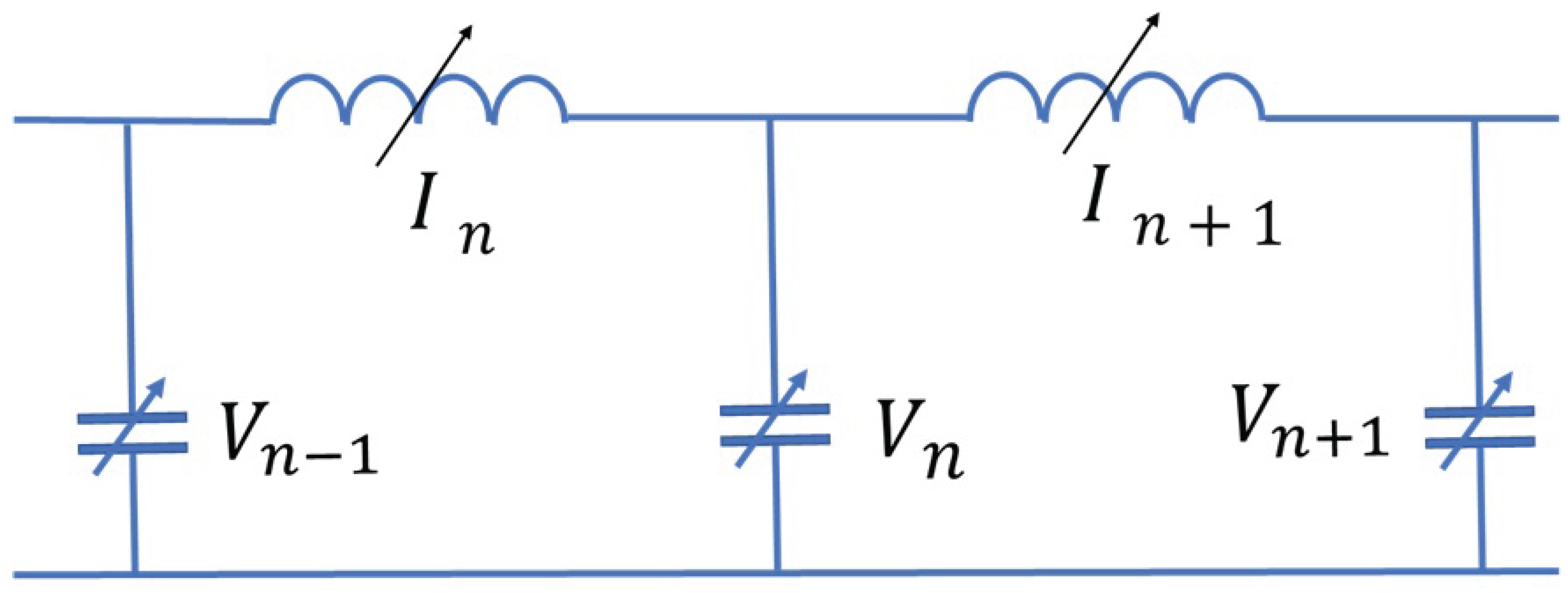
6. The Simple Waves In A Lossless Nonlinear Transmission Line
In the previous part of the paper we considered a lossy nonlinear transmission line. The present section is dedicated to a lossless one. The transmission line constructed from the identical nonlinear inductors and the identical nonlinear capacitors is shown on Figure 2.
We take the capacitors voltages and the currents through the inductors as the dynamical variables. The circuit equations (Kirchhoff laws) are
Further on we’ll consider and as known functions.
In the continuum approximation we treat n as the continuous variable x (we measure distance in the units of the transmission line period) and approximate the finite differences in the r.h.s. of the equations by the first derivatives with respect to x, after which the equations take the form
The simple wave approximation allows to decouple the wave equations into two separate equations for the right- and left-going waves [6,7,8]. In our previous publications we introduced such approximation for Equation (48) for the case of half-nonlinear transmission line (more specifically for the case of JTL [9,10,11]). In the present Section we formulate the simple wave approximation for the general lossless nonlinear transmission line including both the nonlinear inductors and the nonlinear capacitors.
To formulate such approximation let us start from the small amplitude waves on a homogeneous background .
For such waves Equation (48) is simplified to
(for brevity we have discarded lower index 0 in Equation (50)).
The solutions of Equation (50) are right- and left-propagating travelling waves, each depending upon the single variable , propagating with the speed
The voltage and current in the "sound" wave are connected by the equation
where
The simple wave approximation, that is decoupling of (48) into two separate equations for the right- and left-going waves, is achieve by considering V as a function of I (or vice-verse). Then from Equation (48) we obtain
or equivalently
Substituting into (48) we obtain a system of two coupled equations for each of the simple waves
Further on for the sake of definiteness we’ll talk only about the right-going wave which corresponds to taking the sign minus in the r.h.s. of both equations in (56).
The system (56) simplifies in half-nonlinear cases, that is when either the capacitor or the inductor is linear. In the first case (const)
and (56a) becomes closed equation for the current
Instead of (56b) we can use equation
Talking about this case we have in mind first and foremost the Josephson transmission line. Both Josephson laws can be presented as
thus we obtain
However, the fully nonlinear case can also be treated easily. If we consider the initial value problem
the solution of Equation (56) can be obtained by inspection [13]
where
The simple wave approximation (56) can be applied also to Equation (4). In fact, the dissipative terms in the equation determine the profile of the shock. On the other hand, if we want to study the formation of the shocks, then assuming these terms to be in some sense small, we can ignore the influence of the dissipation on the process of the formation (until we don’t approach to close to the singularity of the dissipationless equation). Thus ignoring the dissipation in (4) we may rewrite the equation in the form
which coincides with Equation (48) if we put
After that we can apply the procedure presented above in this Section.
Now let us forget about the dissipation and consider the strictly disssipationless case. If we want to study the profile of the travelling waved in such case, additional complication (with respect to the lossy case) arises. In the latter case we started from considering the discrete transmission line, but the presence of the dissipation introduced the space scale into the system, and this scale was implicitly assumed to be much larger than the period of the line [12]. This allowed us to use the continuum approximation, actually ignoring the discrete nature of the system. For the lossless case the scale of the localized travelling wave is determined by the period of the transmission line [9,10,11]. This makes the continuum approximation inadequate and we introduced the quasi-continuum approximation [9], which corresponds to approximating the finite differences in the r.h.s. of the equations (47) by the two first terms in the Taylor expansion [9,10,11]. Thus instead of Equation (48) we obtain
We studied in details the travelling waves described by these equations for the case of half-nonlinear transmission line (more specifically for the case of JTL [9,10,11]). In distinction to the lossy case, where the travelling waves turn out to be the shocks, in the lossless case the travelling waves turn out to be the kinks and the solitons.
We also studied (with much less details) the formation of the solitons and the kinks via introducing the simple wave approximation for the JTL. Now we want to formulate the simple wave approximation for the general lossless nonlinear transmission line including both the nonlinear inductors and the nonlinear capacitors on top of the quasi-linear approximation.
One must understand that Equation (48) (and hence Equation (56) can describe the formation of the kinks and the solitons (until we don’t approach to close to the singularities of the equations). Our present aim is to formulate the approximation which will describe both the formation of the kinks and the solitons and their profiles.
Starting from Equation (67) and repeating the process which led from (48) to (56) we obtain instead of the latter
Let us apply thus improved simple wave approximation to the JTL. In this case instead of Equation (58) we obtain
If we make an additional assumption , Equation (69) can be written down as [9]
where we have ignored the term proportional to . Looking at Equation (70) we recognize the modified Korteweg-de Vries (mKdV) equation [14].
On the other hand, considering small variations of the current on the constant background presented by Equation (49a), from (70) we obtain [9]
where we have ignored the term proportional to . Looking at Equation (71) we recognize the Korteweg-de Vries (KdV) equation [14].
To conclude we state that we obtained the exact analytical expressions for the profile of the shock waves (both the current and the voltage) in half-nonlinear transmission lines for the appropriate values of the parameters. We also formulated the simple wave approximation for the lossless discrete nonlinear transmission line.
References
- G. B. Whitham, Linear and Nonlinear Waves, John Wiley & Sons Inc., New York (1999).
- E. Kengne, W. M. E. Kengne, W. M. Liu, L. Q. English, and B. A. Malomed, Phys. Rep. 982, 1 (2022).
- R. Landauer, IBM J. Res. Dev. 4, 391 (1960).
- S. T. Peng and R. Landauer, IBM J. Res. Dev. 17, 299 (1973).
- E. Kogan, Phys. Stat. Sol. (b), 262, 2400335 (2025).
- L. D. Landau and E. M. Lifshitz, Fluid Mechanics: Landau and Lifshitz: Course of Theoretical Physics, Volume 6 (Vol. 6), Elsevier (2013).
- M. I. Rabinovich and D. I. Trubetskov, Oscillations and Waves, Kluwer Academic Publishers, Dordrecht / Boston / London (1989).
- M. B. Vinogradova, O. V. M. B. Vinogradova, O. V. Rudenko and A. P. Sukhorukov, The Wave Theory, Nauka Publishers, Moscow (1990).
- E. Kogan, Phys. Stat. Sol. (b) 259, 2200160 (2022).
- E. Kogan, Phys. Stat. Sol. (b) 260, 2200475 (2023).
- E. Kogan, Phys. Stat. Sol. (b) 261, 2300336 (2024).
- E. Kogan, J. E. Kogan, J. Appl. Phys. 130, 013903 (2021).
- J. D. Logan, An introduction to nonlinear partial differential equations (Second Edition), A John Wiley & Sons, Inc. Publication, Hoboken, New Jersey, 2008.
- P. G. Drazin and R. S. Johnson, Solitons: An introduction. Vol. 2., Cambridge university press, 1989.
Figure 1.
Lossy nonlinear transmission line
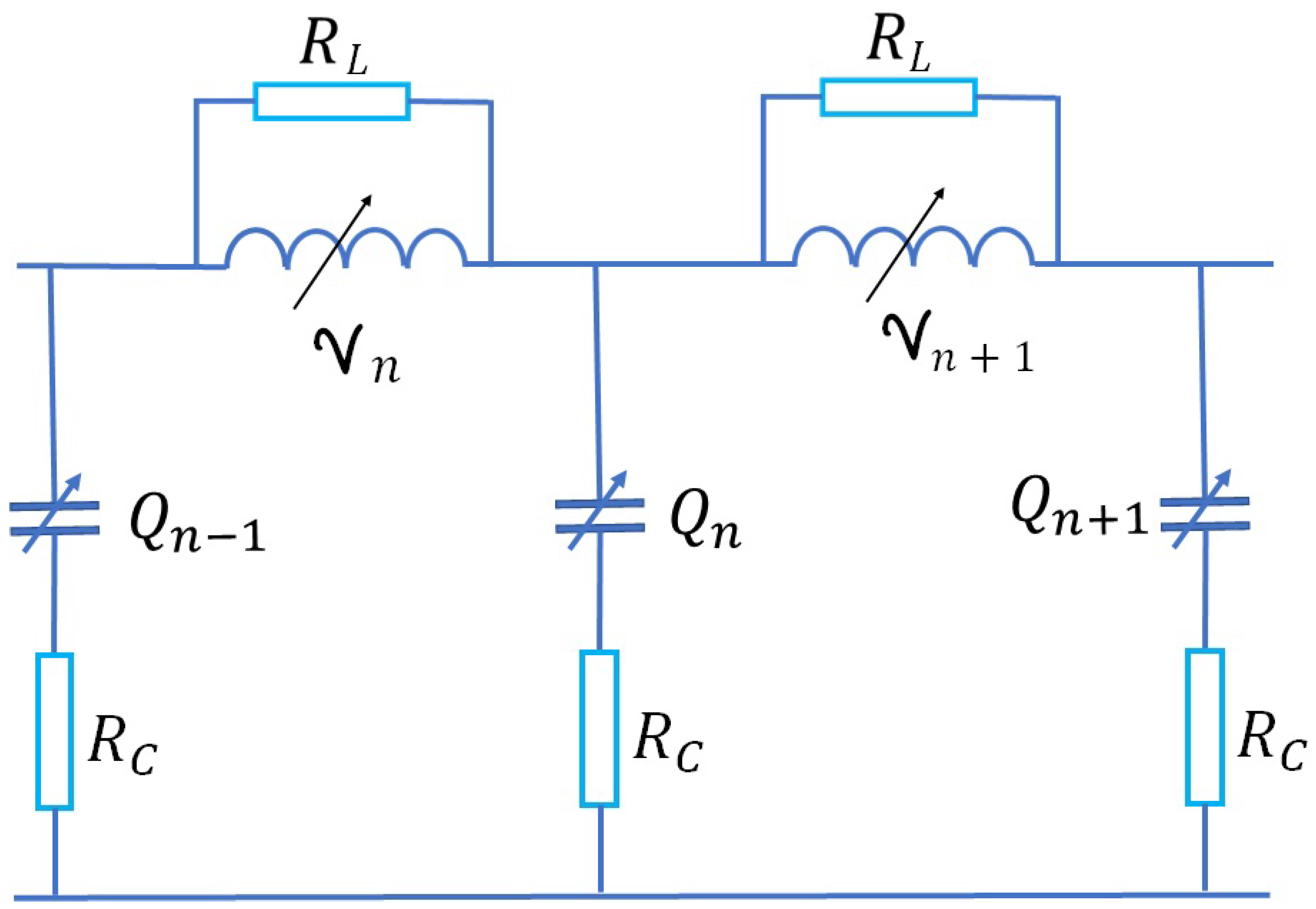
Figure 2.
Lossless nonlinear transmission line
Disclaimer/Publisher’s Note: The statements, opinions and data contained in all publications are solely those of the individual author(s) and contributor(s) and not of MDPI and/or the editor(s). MDPI and/or the editor(s) disclaim responsibility for any injury to people or property resulting from any ideas, methods, instructions or products referred to in the content. |
© 2025 by the authors. Licensee MDPI, Basel, Switzerland. This article is an open access article distributed under the terms and conditions of the Creative Commons Attribution (CC BY) license (http://creativecommons.org/licenses/by/4.0/).
Copyright: This open access article is published under a Creative Commons CC BY 4.0 license, which permit the free download, distribution, and reuse, provided that the author and preprint are cited in any reuse.


