Submitted:
23 July 2025
Posted:
24 July 2025
You are already at the latest version
Abstract
Biorobotics employs principles of natural locomotion to improve robots' mobility. Among various swimming modes, anguilliform locomotion is particularly recognized as an energy-efficient mode that incorporates complex physics. Due to whole-body undulation, the determination of the anguilliform swimmer’s direction is not trivial, and the mechanism of muscle interaction to maintain the desired direction is complex. In this study, the problem of predicting and controlling the gross motion trajectory of a soft robot with anguilliform swimming on the water surface is investigated. The robot consists of a six-segment continuous body, where each segment is actuated with artificial muscles to bend left and right. A DMD-based mode extraction technique is proposed to identify the robot's trajectory, which represents the heading direction. The algorithm, namely CDE DMD, utilizes delay-embedded complex variable states to calculate the future trend of the robot state. For the control, a hypothesis that asymmetric sidewise actuation results in regulation of the swimming direction was investigated using COMSOL Multiphysics® 6.2. The results demonstrate the CDE DMD ability to predict gross motion for various scenarios. The prediction and asymmetric actuation rules can be used to maintain swimming in a straight line, a problem which is known as directional stability.
Keywords:
bionics
; data-driven model
; ML-based robot control
; anguilliform locomotion
; directional stability
1. Introduction
Conventional machines employ rotary motors as the main part of the propulsion system to drive wheels or rotatory fans in ships. On the other hand, nature offers various locomotion mechanisms that are significantly more efficient, especially in complex and unstructured environments. For aquatic locomotion, propulsion in liquid domains, fishes exhibit various modes such as anguilliform, subcarangiform, carangiform, and thunniform [1]. The Lindsey classification of the fish swimming styles counts twelve modes based on the geometry of the moving region of the fish, and body undulation or oscillation [2,3]. Admittedly, drawing a definite border between the modes is not easy because the modes appear to be kinematically analogous. Nevertheless, the anguilliform mode is particularly distinguishable from the other modes because the whole body is engaged in the undulatory motion, containing the rearward-travelling wave that provides propulsion for the swimmer. In this mode of locomotion, fins do not play the major role, and so snake-like anatomies in various ranges from nematodes to eels employ an anguilliform mode for locomotion. This can be used for developing robotic systems intended to navigate fluidic environments in different Reynolds numbers (Re). Biorobotics is a branch of robotics focusing on studying the kinematics of natural locomotion regimes and implementing the principles in actual robots. From the technologists’ point of view, developing or optimizing robots’ performance, e.g., speed or energy consumption, is a provisional achievement. The scalability of anguilliform mode is particularly important when technology limitations do not allow making tiny conventional motors or when the motors increase the total mass, which creates buoyancy and agility problems. Furthermore, scalability, if deciphered by the Re, reflects motion capability in a viscous environment.
One advantage of anguilliform swimming is its energy efficiency in long-distance movements. Maintaining the swimmer’s direction along the desired direction is the first question raised from the control engineering point of view. The problem can be stated as determining the control strategy to make the swimmer follow a straight line. The problem contains complexities that may be translated to observer and actuator control in robotics terms. On one hand, due to whole-body undulation, there is no physically rigid moving point indicating the motion direction. In anguilliform locomotion, the measurements of any positioning sensor [4] will be contaminated with the body undulation. On the other hand, there is no specified primary actuator, like fins, for creating the necessary yaw torques for straight swimming. In fin-based steering, in fish such as sunfish or perch, dorsal, anal, and caudal fins counteract unwanted body rotations to maintain forward motion. Due to the lack of pronounced appendages and body flexibility, directional stability of the slender and elongated fishes, such as eels, lampreys, and larval fishes, relies on kinematics and hydrodynamics. To swim straight, such species may rely on highly symmetric body undulations to produce net forward thrust without lateral deviation [5]. Turning can be seen as a separate problem within the study of anguilliform locomotion. It was shown that snakes twist their bodies inwards and shift their center of mass to reduce their moment of inertia during a turning behavior [6]. In [7], it is reported that an eel performs forward motion or distinctive curling behavior depending on some external electrical stimulation. Nevertheless, they concluded that full control over the eel’s motion (such as the path following problem) is far more complicated. Within fish, swimming locomotion is classified into two generic categories: steady (employed by the fish over relatively long distances at a constant speed) and transient movements [1]. Similarly, the problem of the elongated robots’ navigation can be divided into steady path following and unsteady maneuvers (including turning).
Robots are prone to errors in their initial pose, disturbance within locomotion, as well as actuator and sensor faults. Therefore, the swimming of a robot along a line needs active control, especially over long distances. Various research is devoted to path planning and trajectory following of elongated robots [8,9,10,11]. Multi-body rigid snake robots can rely on angular deflections added on different joints for turning motion, as formulated in [12]. Recently, strategies based on left-right unbalanced amplitude and head steering were experimentally implemented for maneuvering a soft swimming robot [13]. Unlike rotary motors that can rotate to any angle as the reference zero around which the rotor oscillates, soft actuators commonly have a fixed nominal position corresponding to the straight nominal state of the fish robot. Therefore, finding a method for regulating the soft robot’s swimming direction is essential.
Machine learning (ML) techniques are extensively explored to handle different problems, such as gait optimization [14] and analysis of mode shapes as the result of the interaction of the soft body with the surrounding water [15,16] for anguilliform swimming robots. The dynamic mode decomposition (DMD) is a data-driven ML technique that is powerful in uncovering coherent structures within fluid flows and mechanical vibrations. Various variants of the DMD algorithm have been developed for forecasting and identification in different scientific applications. The delay embedding technique has demonstrated the capability of decomposing interconnected dynamics, like separating waves and turbulence in fluid dynamics [17,18]. The complex delay-embedded method, CDE DMD, has shown the capability of decomposing the underlying modes of anguilliform swimming from experimental data obtained by tracking markers on the midline of a soft eel robot [19]. It was shown that the method isolates the travelling wave dynamics as the result of inherent linear (in the sense of DMD) modes.
This study is focused on the directional control of anguilliform swimming of a pneumatic soft robot. The CDE DMD is explored and adapted to identify and predict the swimmer’s gross motion. The investigated question is limited to proposing a solution to maintain straight swimming with small deviations from the nominal working point. A simulation study using COMSOL Multiphysics® 6.2 (COMSOL AB, Stockholm, Sweden) was performed, especially to evaluate the directional variation based on unbalanced forcing with different right-left maximum pressures.
The remaining parts of this article are organized as follows. In Section 2.1, first, the undulatory motion and the problem of directional stability in anguilliform swimming are explained. Then, in Section 2.2, the method of CDE DMD and the online prediction formula are derived. Section 2.3 is devoted to explaining the actuation method proposed for generating the control input. The computation and simulation results are presented in Section 3. The prediction formula is first calculated and tested on some open-loop scenarios. Then, it is shown that the predictor can be used in a closed-loop control to provide a straight swimming and regulation of the initial state error. Discussion and conclusions are summarized in Section 4 and Section 5.
2. Materials and Methods
2.1. Problem Statement
Ideally, inspired by the swimming of salamanders, the simplest kinematics of the travelling waves in anguilliform locomotion can be described by a backward-moving sinusoidal wave like
Where is the undulation amplitude, is the wavelength, and is the wave velocity along the swimming axis . In steady swimming, the velocity and amplitude have constant values. Nevertheless, achieving such ideal movement is practically very hard due to the imperfect mechanical structure of robots, along with external disturbances. An illustration of the anguilliform swimming kinematics is schematically shown in Figure 1. For comparison, a stable straight motion is shown in Figure 1(a), while in Figure 1(b) and 1(c) the swimming involves a uniform tilting to the left and right, respectively. In this case, the undulation time is T, and the tilting involves nearly yaw during the period. Although the deviation angle is considerable, in reality, its effects appear very slowly because the undulation period for swimming in water contains low frequencies in the range of 100 Hz. This fact makes the control problem challenging from a control engineering point of view. The challenge is to detect (or identify) the direction deviation in a short time within a small portion of the period to be able to counteract it by a feedback controller gain. Let it aside that the presence of extra modes in practice does make the problem more complicated. A quick detection of a deviation angle, potentially, provides the necessary signal for the steering mechanism to act against the deviation and stabilize the forward motion. Otherwise, if the observer requires some number of undulations to estimate the tendency, the control will encounter a time delay due to measurement time as well as fluid dynamics resistance of the water.
The next problem concerning stable swimming is related to the actuation for control purposes. A mechanism is required to maintain efficient forward swimming as well as direction adjustments simultaneously. It is hypothesized that regulating the muscle forces of one side results in a sidewise tendency or yaw motion. However, due to the high density of water, the swimming capability of soft robots is not easily achieved, and asymmetric actuator force should be minimized. In order to get insight into the effect of unbalanced actuation and find effective parameters, a particle tracking simulation using COMSOL is proposed.
2.2. The CDE DMD
The method involves tracking data of discrete markers distributed uniformly on the midline of the swimmer’s body. Suppose the state vector at time is shown by a complex variable, composed of the lateral position and filtered velocity of s digitized points of the robot midline as
Following the technique of delay embedding, the Hankel matrix is constructed by embedding delayed coordinates as follows
As in the snapshot syntax, the matrix is denoted by its columns representing the kth column of H.
Then, a linear operator mapping snapshots of the system dynamics one timestep forward, fundamentally a linear approximation of the Koopman operator, , is considered as
Based on the DMD approach, the best solution can be obtained by solving the matrix equation
where and . The matrix is decomposed to left singular vector, , diagonal matrix of singular values, , and the Hermitian transpose of right singular vectors using a singular value decomposition (SVD) as
Where ‘.*’ denotes the Hermitian transpose. Supposing the SVD calculation provides the matrices as
where are chosen the leading singular values. Therefore, a modal decomposition can be expressed as
The pseudoinverse matrix, , satisfying is obtained using
In the CDE DMD analysis of anguilliform locomotion, we are interested in particular modes that compose interesting physical motions, including the pure backward-travelling waves, stationary waves, and, in this research, the rigid or gross motion. Supposing the physics of interest is presented, e.g., by and , the pseudoinverse matrix can be partitioned as
So that
Thus, the linear operator, , corresponding to the specified modes is readily calculated as
Note that relates the current state vector in the embedded coordinates to the next approximate snapshot, shown by , corresponding to the relevant modes as in
An eigendecomposition of is computationally viable, satisfying:
In DMD, the eigenmodes are measured by eigen decomposition of a reduced-order matrix. To measure exclusively the first term, , the update rule can be written with the first rows as
When the neutral dynamics, representing rigid-body motion, has two eigenvalues equal to one, the prediction formula can be simplified as follows.
The memory allocation for online measurement of is schematically shown in Figure 2. The current value, , is updated using the , measured at the time , and the previous value, , in a memory stacking manner. Then, the update rule is used in (16) to calculate the estimated future value .
2.3. The Actuation Mechanism
The previous section provides a state estimator or observer that can be used for control purposes using a control rule. In this section, an actuation method for implementing the controller is proposed. A model of the system is shown in Figure 3, which shows the actual mesh used within the COMSOL simulation, similar to the model given in [15]. The robot body is shown by green elements with additional annotations giving the dimensional and forcing information. The robot has six segments, and each segment contains lateral contracting type McKibben actuators that enable the segment to bend to the right or left. The actuator forces are the external forces shown by the red arrows, and their values are related to the actuation sequence, represented in Figure 4, and the contraction force obtained by the pressurizing, which are shown as and for the right and left sides. Thus, for segment number i=1 to 6, the forces can be written as
In the uncontrolled system is supposed to be constant. However, for an unbalanced actuation, we suppose a slightly reduced pressure, , and a direction parameter so that
To investigate how the slightly unbalanced forcing may affect the material transport within a computational fluid dynamics (CFD) scope, a COMSOL particle tracing simulation known as particle tracing for fluid flow (known as fluid-particle tracing, FPT) is performed. Note that the unbalance factor can be related to a heuristic control rule expressed as
, where ℜ refers to the real part of the complex variable, sgn refers to the sign function, and K is the control gain for the simple case of a linear proportional controller.
3. Results
Unlike Eulerian methods, which observe flow at fixed spatial points, FPT follows individual particles, providing direct insight into the material transport. The FPT simulation results for three (open-loop) scenarios are shown in Figure 5. For meshing, the physics-controlled coarse mesh was used for the whole domain. The integrated physics includes laminar flow (SPF), solid mechanics (for the robot body), moving mesh (for fluid domain), fluid-structure interaction (FSI), and the FPT. Water physical properties were chosen as the properties of the 0.2 mm radius particles so that they represent the material flow of water, with the Stokes drag law. The simulation is arranged with two steps: Study 1 and Study 2 in COMSOL. First, in Study 1, the time-dependent analysis is performed without computing the particle tracing. In Study 2, only the FPT is solved. In this step, the results of the time-dependent analysis from the previous step, Study 1, are used as the values of variables not solved for.
The particles are released from a grid uniformly as shown in the plots at the top of Figure 5. The simulation was performed for three cases (including balanced forcing for straight motion, and unbalanced forcing for left and right tendency), and the results are saved using image sequences. The time collapsed between the vertically arranged snapshots is 0.88 s, and the colors simply represent the index of the particles to make the tracing more visible. The robot velocity is 0.033 m/s, and the undulation frequency is 1.1 s.
In Figure 5(a), the results for balanced forcing are shown. The sequence of the snapshots, which is arranged from top to down, shows a uniform and visually symmetric distribution. In contrast, in the unbalanced actuation shown in Figure 5(b), with accentuating left forces, and Figure 5(c), accentuating right, an asymmetric material displacement is observed at the downstream.
3.1. The CDE DMD
In this section, the CDE DMD method is used for the prediction and control of the gross lateral motion of the robot. The system, as shown in Figure 3, is spatially discretized to seven points, A1 to A7, equally distributed on the midline of the robot’s continuous body. To evaluate the capability of the proposed method in the estimation of the robot’s gross motion, first, some state data is assembled of the Hankel matrix given in (3). The state vector, shown by the complex variable within the manuscript, includes the lateral position and velocity, which can be obtained by differentiation of the position data. Different open-loop arbitrary scenarios are considered where and the control input takes constant values like
According to (18), when we will have and . Likewise, when we will have and , and when symmetric actuation is provided as . One advantage of this input is the feasibility of implementation using standard industrial pneumatic components. A pneumatic regulator can be used to provide from the nominal pressure, 600 [KPa]. Switching pneumatic valves, which are smaller and much less expensive than analog pressure control valves, are used to guide the discrete input pressures to the actuators. Next, some data is required to assemble the data matrices and perform the calculations (also known as training within ML terminology). An arbitrary input shown in Figure 6 was implemented to randomly manipulate the system. At this point, any arbitrarily varying input resulting in casual navigation with a rich gross motion effect is sufficient (Note that high frequency inputs may not yield a noticeable gross motion). The system response, i.e., the states of the discrete points on the robot midline, is shown in Figure 7. The position data is obviously showing a noticeable overall motion, in addition to oscillations. The modal decomposition (8) is used to separate the different physics by projecting the data into a modal space. Visualization of the modes’ contribution, also known as the reconstruction process, is a tool to reveal the effect of the modes and distinguish the different underlying physics.
The modal decomposition results are shown in Figure 8. The linear oscillations, shown by the blue curve, demonstrate the pure undulation, which contains the main drive in the anguilliform locomotion. The gross motion, which is of more interest in this work, is the next major part of the signals and is shown by the black curve. The graphs show that the curve provides a good approximation of the gross motion. Note that the superposition of the linear oscillations and the gross motion provides a form of reduced-order approximation (reconstruction) of the original data.
To investigate this issue numerically, the superposition of the linear oscillations and the gross motion is plotted in Figure 9. The figure shows that the errors, which are associated with higher modes, demonstrate small amplitudes compared to the main data. This analysis reveals the contribution of modes in the pure undulation, as well as a drift or trend attributed to rigid-body-like motion, namely gross motion of the robot.
The results of the CDE DMD predictor given by (16) are shown in Figure 10. From an ML point of view, the method manipulates the data in an unsupervised manner. In fact, the CDE DMD algorithm extracts the existing modes in the dynamics from the data matrix. Note that if the data does not contain the mode information (e.g., in case the data is collected from a short straight motion of the robot in this work), DMD techniques might not find the mode.
Similar to the mechanical vibrations, if an input is not rich enough, a mode may not be excited enough to be detected by data-driven model discovery methods. Another interesting topic in the arena of ML is the performance of the algorithm on unseen data. Employing the ML terminology, the previous data (represented in Figure 7) can be seen as the training data. The data was used to measure the hyperparameters of (16). Then, in the next step, a different maneuvering scenario with an input signal given in Figure 11 is used to evaluate the capability of the algorithm in identifying the gross motion within unseen scenarios. In this case, the algorithm updates a data window (as in Figure 2) from the current data, and then utilizes the pretrained model (16) to predict the trace shown as CDE DMD gross motion in Figure 12.
For the closed-loop control, the linear gain in (19) is heuristically selected as follows. As the corresponds to the position of the middle point (A4), a control term like is used to make up for the distance error. Additionally, another term is required to react against the orientation error. The angle of the robot can be related to which corresponds to the position of two points A1 and A7 Therefore, the controller is expressed as
This control can be seen as a simple bioinspired control law [20] for steering right or left. Analogous to the step response in classical control of linear systems, the closed-loop system performance can be demonstrated by considering a non-zero initial condition for the position of the robot. Figure 13 shows an example scenario of the controlled system using (21) with and . Note that the oscillation around the zero (shown by the dashed line) is the desired objective because it represents swimming in the line. However, when the robot has a non-zero initial angle to the line, the initial position of the discrete points will have a non-zero initial value in the beginning, and the controller compensates for this error. Similarly, in the other scenario shown in Figure 14, at the initial time, there is a distance error concerning the zero line. The results show that the controller provides the error zeroing necessary for navigation in the desired line.
4. Discussion
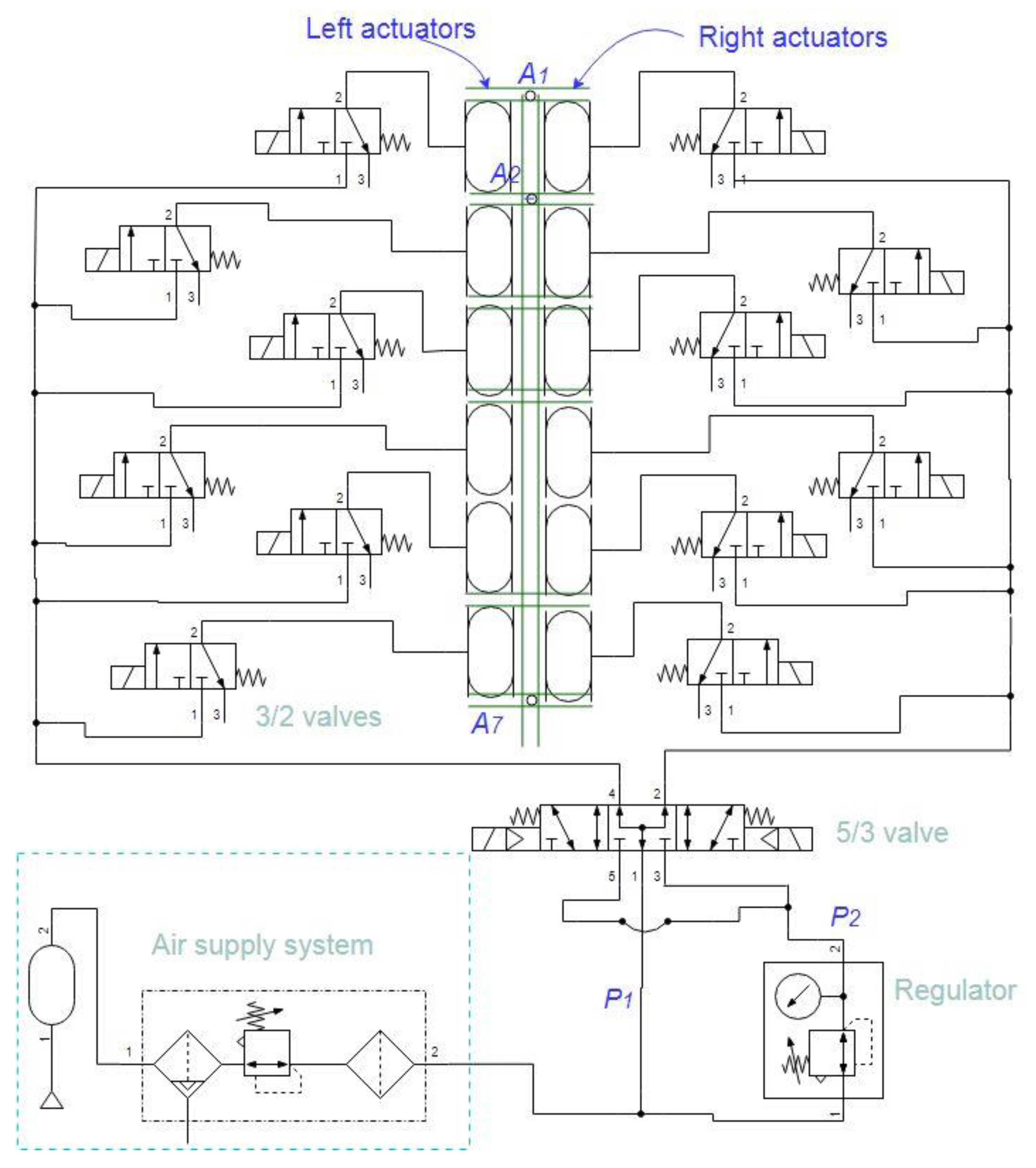
In this study, different open-loop and closed-loop scenarios were analyzed to evaluate the gross motion prediction capability of the CDE DMD method. Within fish locomotion studies, the ability to swim in a straight line is known as directional stability. In comparison with robotics terminology, the directional stability can be related to trajectory following, with the difference that the desired trajectory is a straight line, and conceptually, less position error is expected. Commonly, within robot path following, regular shapes like a square or a circle are considered as the desired path, and the robot is controlled to approximately follow the path with generally tolerable position errors. Furthermore, unlike sharp turns that can be seen as transient curling behavior, the directional stability is associated with steady swimming. The proposed control is physically achieved with a small pressure adjustment, shown in Figure 15. The robot is shown schematically, and the pneumatic control components are shown by the standard symbols. Each segment is controlled by two 3/2 valves to bend to the right or left.
The 3/2 valves are controlled by the sequential signal given in Figure 4. The directional control is performed by the 5/3 valve, which provides the pressure for the 3/2 valves related to each side of the robot. An air supply delivers the nominal pressure, P1, and a regulator provides the P2 pressure for the direction control. The control rule given in (21) is given as the control signal to the 5/3 valve. The three-digit values are to select one of the three possible states of the valve using the solenoids. The simulation results show that the controller provides regulating signals that are practically feasible in hardware implementation. With an initial pose error, the controller, after approximately 60 s, settles the error. The prediction rule acts as a data-driven observer for tracing the robot. The open-loop simulations indicate that the prediction can be used for drawing a trace that approximately shows the overall trace of the robot trajectory. In soft robots and natural anguilliform swimmers, in contrast to rigid robots, which can rely on joint sensors, positioning and tracking the swimmer is complex. The proposed algorithm can be used for tracking or positioning, with or without navigation control purposes.
5. Conclusions
This study focused on the problem of directional heading path prediction and control in anguilliform locomotion of a continuous robot. We followed a bionic approach, where the control problem is viewed as directional control inspired by the two separate navigation behaviors of fish, curling and stable swimming with asymmetric actuation forces. A DMD-based algorithm is proposed to predict the swimmer’s gross motion, which can then be used for navigation purposes. The results show that the algorithm, namely CDE DMD, reveals the trend line associated with the robot’s gross motion, with both training and unseen data sets. Furthermore, a heuristic controller was proposed based on the prediction model. It is concluded that a small difference between the maximum forces of the lateral sides generates asymmetric material movements that can be utilized for achieving directional stability in anguilliform swimming using the CDE DMD method. The results are of special importance in long-distance operations of untethered anguilliform swimming robots, while sharp curling for local navigation remains a future research topic.
Author Contributions
Conceptualization, M.S. and H.W.; methodology, M.S.; software, M.S.; validation, M.S. and H.W.; formal analysis, M.S.; investigation, M.S. and H.W.; resources, M.S. and H.W.; data curation, M.S. and H.W.; writing—original draft preparation, M.S.; writing—review and editing, H.W.; visualization, M.S.; supervision, H.W.; project administration, M.S. and H.W.; funding acquisition, H.W. All authors have read and agreed to the published version of the manuscript.
Funding
This research received no external funding.
Institutional Review Board Statement
Not applicable.
Informed Consent Statement
Not applicable.
Data Availability Statement
The original contributions presented in the study are included in the article; further inquiries can be directed to the corresponding author.
Conflicts of Interest
The authors declare no conflicts of interest.
Abbreviations
The following abbreviations are used in this manuscript:
| CDE | Complex delay embedding |
| CFD | Computational fluid dynamics |
| DMD | Dynamic mode decomposition |
| FPT | Fluid-particle tracing |
| FSI | Fluid–solid interaction |
| ML | Machine learning |
| Re | Reynolds number |
| SPF | Single-phase flow |
| SVD | Singular value decomposition |
References
- Sfakiotakis, M.; Lane, D.M.; Davies, J.B.C. Review of fish swimming modes for aquatic locomotion. IEEE Journal of oceanic engineering 2002, 24, 237-252. [CrossRef]
- Lindsey, C.C. Form, function, and locomotory habits in fish. In Fish physiology; Elsevier: 1978; Volume 7, pp. 1-100.
- Satoi, D.; Hagiwara, M.; Uemoto, A.; Nakadai, H.; Hoshino, J.J.A.T.o.G. Unified motion planner for fishes with various swimming styles. 2016, 35, 1-15. [CrossRef]
- Alexandris, C.; Papageorgas, P.; Piromalis, D. Positioning systems for unmanned underwater vehicles: A comprehensive review. Applied Sciences 2024, 14, 9671. [CrossRef]
- Tytell, E.D.; Lauder, G.V. The hydrodynamics of eel swimming: I. Wake structure. Journal of Experimental Biology 2004, 207, 1825-1841. [CrossRef]
- Gregorio, E.; Godoy-Diana, R.; Herrel, A. Turning without Fins: How Snakes Achieve High Maneuverability While Swimming. 2025.
- Yu, L.; Lai, J.; Huang, J.; Liu, H.; Pi, X. Wireless motion control of a swimming eel-machine hybrid robot. Bioinspiration & Biomimetics 2025, 20, 036010. [CrossRef]
- Xu, J.-X.; Niu, X.-L.; Ren, Q.-Y.; Wang, Q.-G. Collision-free motion planning for an Anguilliform robotic fish. In Proceedings of the 2012 IEEE International Symposium on Industrial Electronics, 2012; pp. 1268-1273.
- Melsaac, K.; Ostrowski, J.P. A geometric approach to anguilliform locomotion: modelling of an underwater eel robot. In Proceedings of the Proceedings 1999 IEEE International Conference on Robotics and Automation (Cat. No. 99CH36288C), 1999; pp. 2843-2848.
- Raj, A.; Kumar, A.; Thakur, A. Automated locomotion parameter tuning for an anguilliform-inspired robot. In Proceedings of the 2016 IEEE International Conference on Systems, Man, and Cybernetics (SMC), 2016; pp. 002564-002569.
- Thati, S.K.; Raj, A.; Thakur, A. Optimal and Dynamically Feasible Path Planning for an Anguilliform Fish-Inspired Robot in Presence of Obstacles. In Proceedings of the ASME 2018 International Design Engineering Technical Conferences and Computers and Information in Engineering Conference, 2018.
- Niu, X.; Xu, J.; Ren, Q.; Wang, Q. Locomotion generation and motion library design for an anguilliform robotic fish. Journal of Bionic Engineering 2013, 10, 251-264. [CrossRef]
- Shi, H.; Meng, Y.; Cui, W.; Rao, M.; Wang, S.; Xie, Y. Biomimetic Underwater Soft Snake Robot: Self-Motion Sensing and Online Gait Control. IEEE Transactions on Robotics 2025. [CrossRef]
- Hameed, I.; Chao, X.; Navarro-Alarcon, D.; Jing, X. Deep reinforcement learning enabling a BCFbot to learn various undulatory patterns. Ocean Engineering 2025, 320, 120322. [CrossRef]
- Sayahkarajy, M.; Witte, H. Analysis of Robot–Environment Interaction Modes in Anguilliform Locomotion of a New Soft Eel Robot. Actuators 2024, 13, 406. [CrossRef]
- Sayahkarajy, M.; Witte, H. Temporal Evolution of the Hydrodynamics of a Swimming Eel Robot Using Sparse Identification: SINDy-DMD. J — Multidisciplinary Scientific Journal 2025. [CrossRef]
- Chávez-Dorado, J.; Scherl, I.; DiBenedetto, M. Wave and turbulence separation using dynamic mode decomposition. Journal of Atmospheric Oceanic Technology 2025, 42, 509-526. [CrossRef]
- Asada, H.; Kawai, S. Exact parallelized dynamic mode decomposition with Hankel matrix for large-scale flow data. Theoretical Computational Fluid Dynamics 2025, 39, 8. [CrossRef]
- Sayahkarajy, M.; Witte, H. Empirical Data-Driven Linear Model of a Swimming Robot Using the Complex Delay-Embedding DMD Technique. 2025, 10, 60. [CrossRef]
- Wang, J.; Chen, H. BSAS: Beetle swarm antennae search algorithm for optimization problems. arXiv preprint arXiv:.10470 2018.
Figure 1.
Illustration of anguilliform swimming kinematics within an undulation period, T: (a) Motion in a straight line; (b) Swimming with left-tilting tendency; (c) Right-tilting motion. The blue line represents the initial state, and the dashed-dot represents the (desired) position in straight motion.
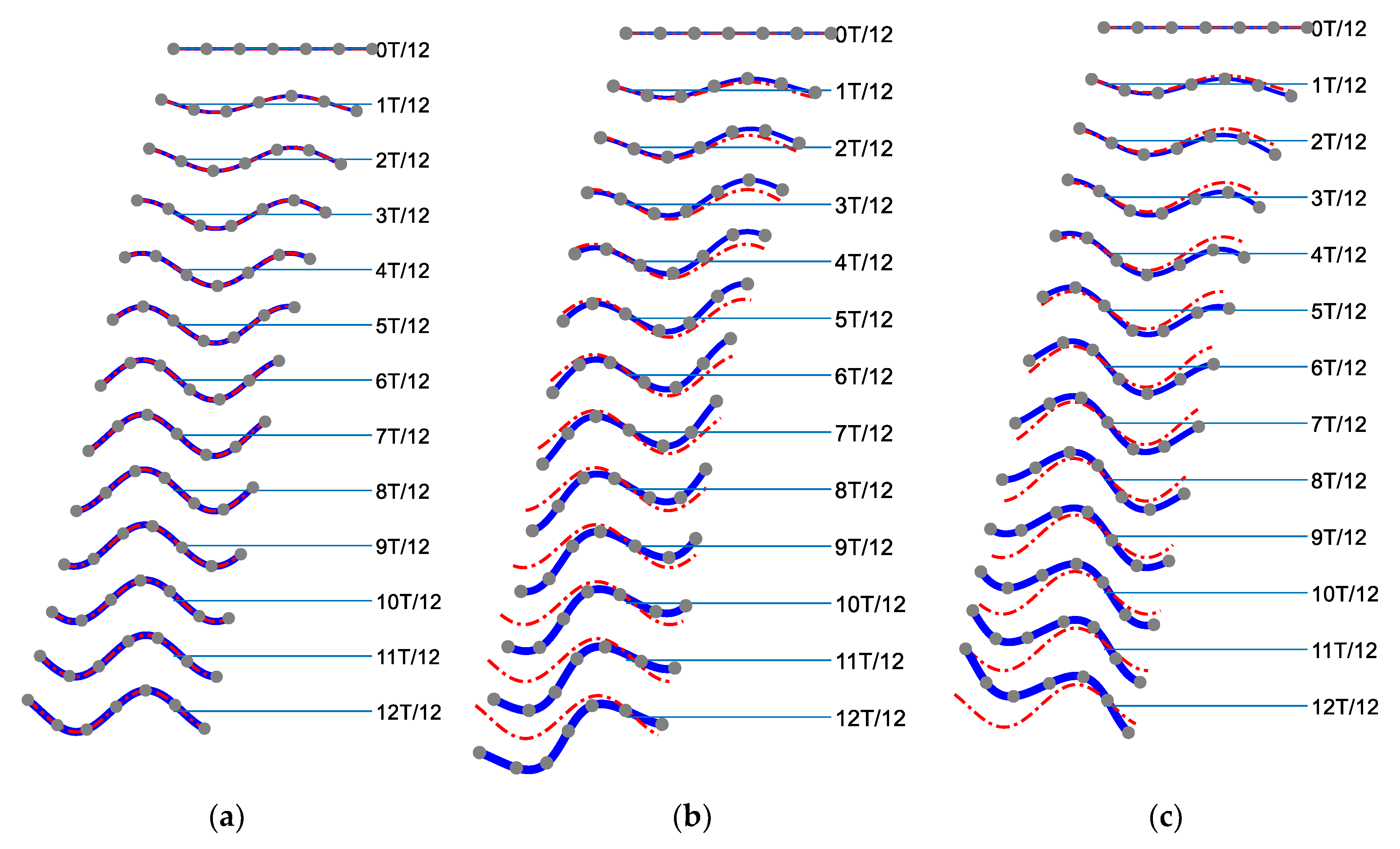
Figure 2.
Memory stacking to update .
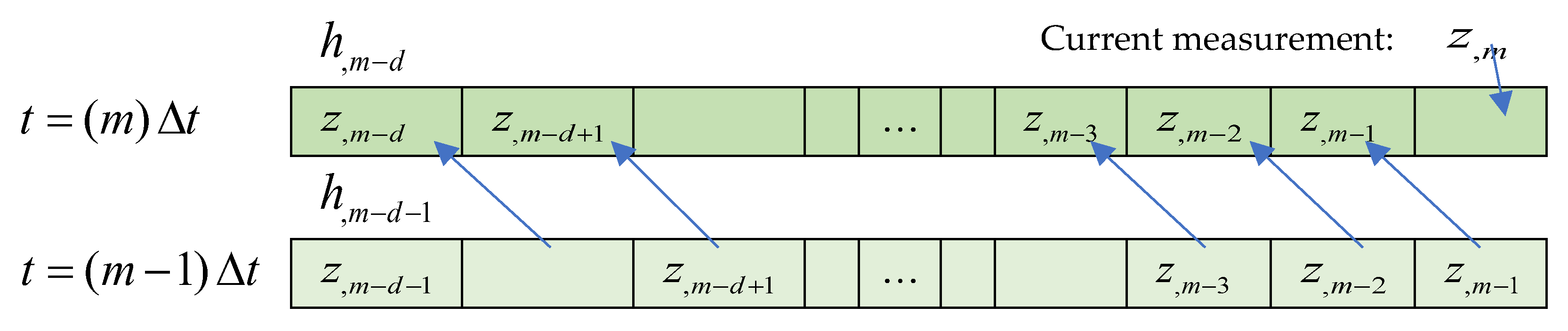
Figure 3.
The simulation model: (a) Three-dimensional view; (b) The finite element mesh, dimensions, and forces. The dimensions are given in mm, and red arrows show the actuators’ forces for the six segments. The small blue circles represent motion tracking points from the head (A1) to the distal segment (A7).
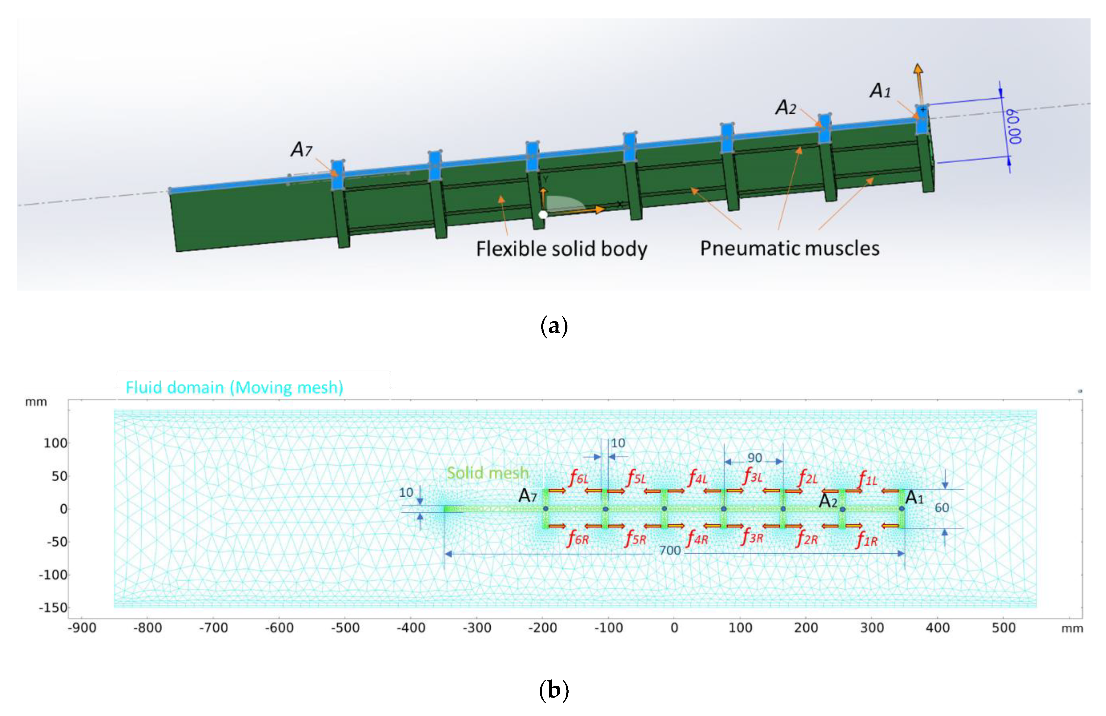
Figure 4.
The segmental actuation sequence for a travelling wave along the robot body.
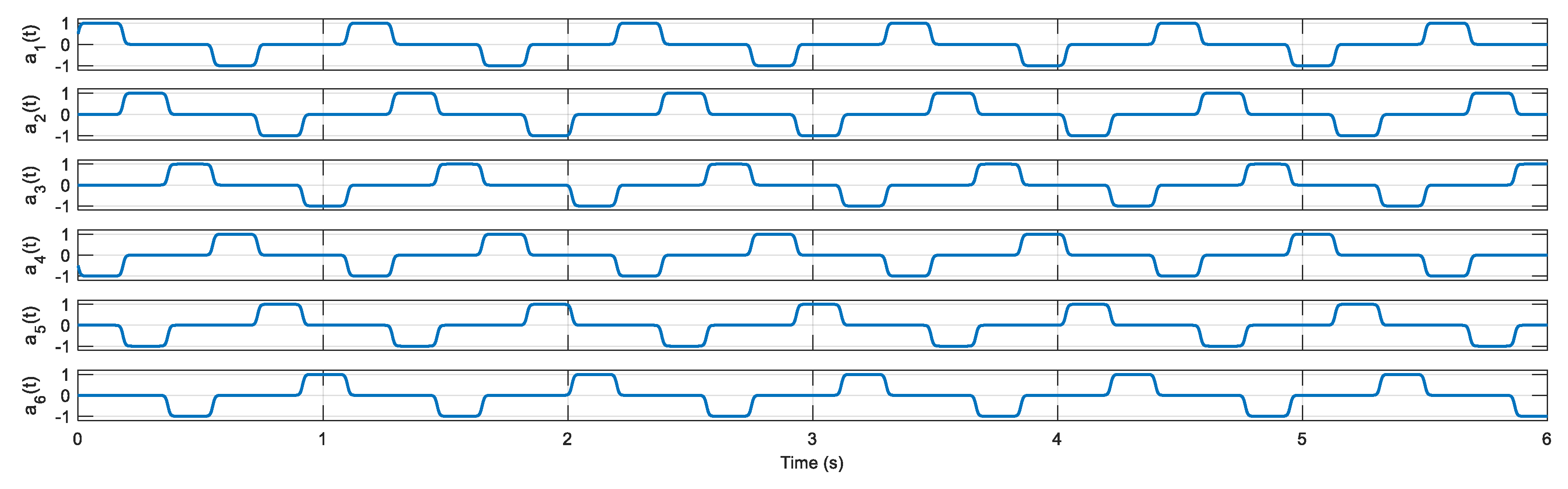
Figure 5.
The FPT simulation results: (a) Motion in a straight line; (b) Swimming with left-tilting tendency (); (c) Right-tilting motion (). The color bar represents the particle indices.
Figure 5.
The FPT simulation results: (a) Motion in a straight line; (b) Swimming with left-tilting tendency (); (c) Right-tilting motion (). The color bar represents the particle indices.
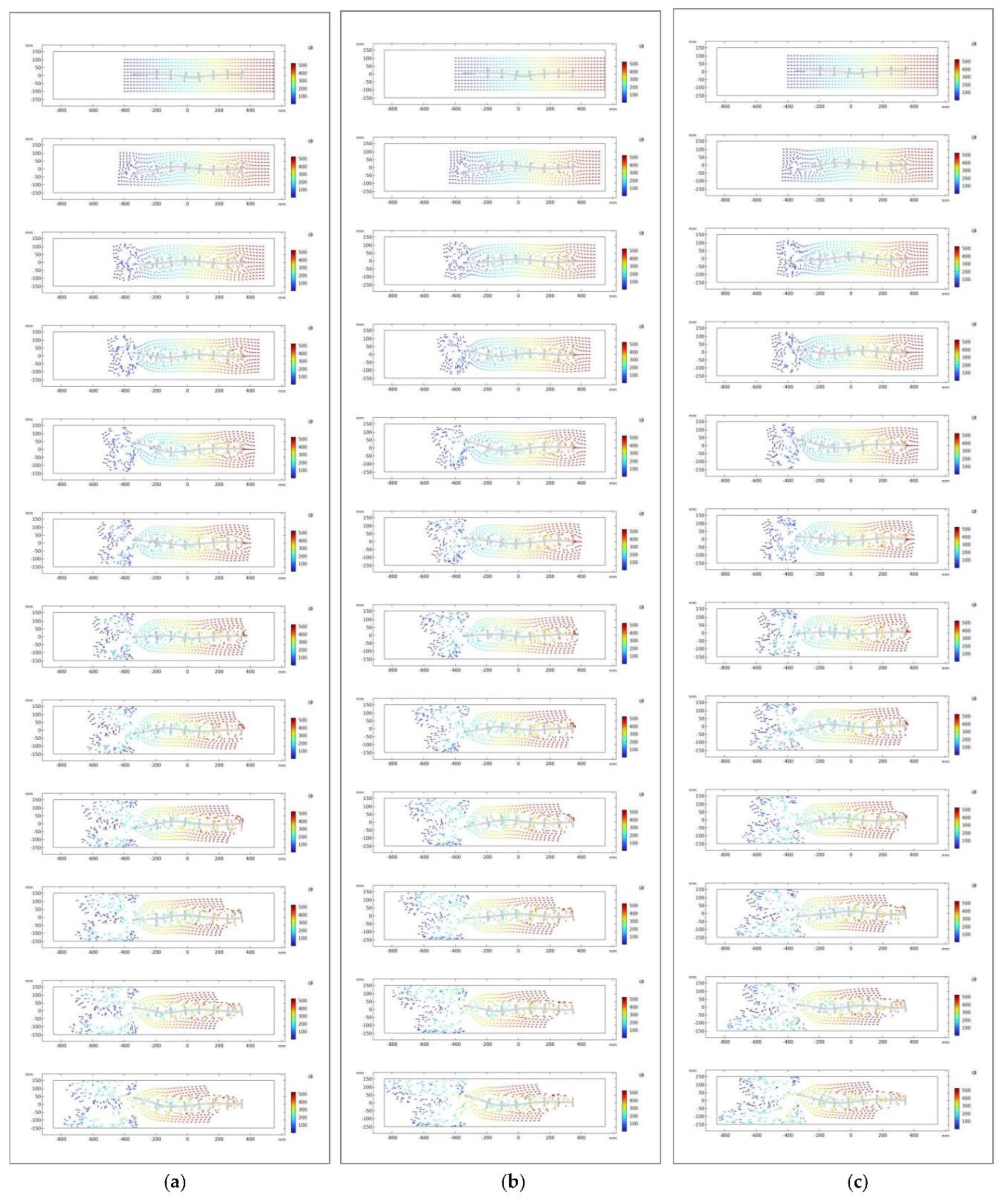
Figure 6.
The arbitrary input used in the first scenario.
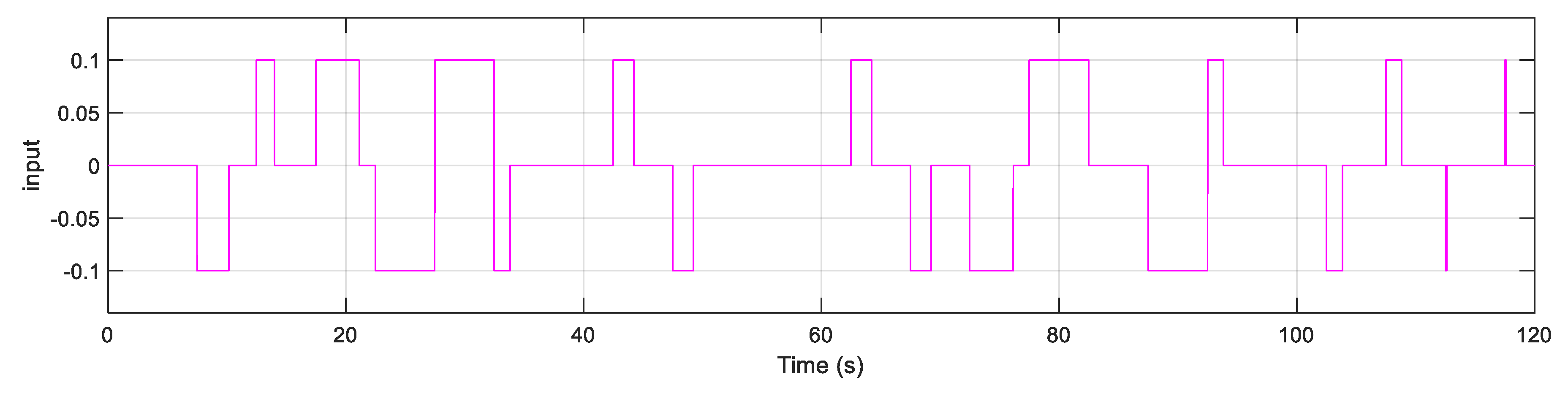
Figure 7.
The lateral position and velocity data of the tracking points, A1 to A7.
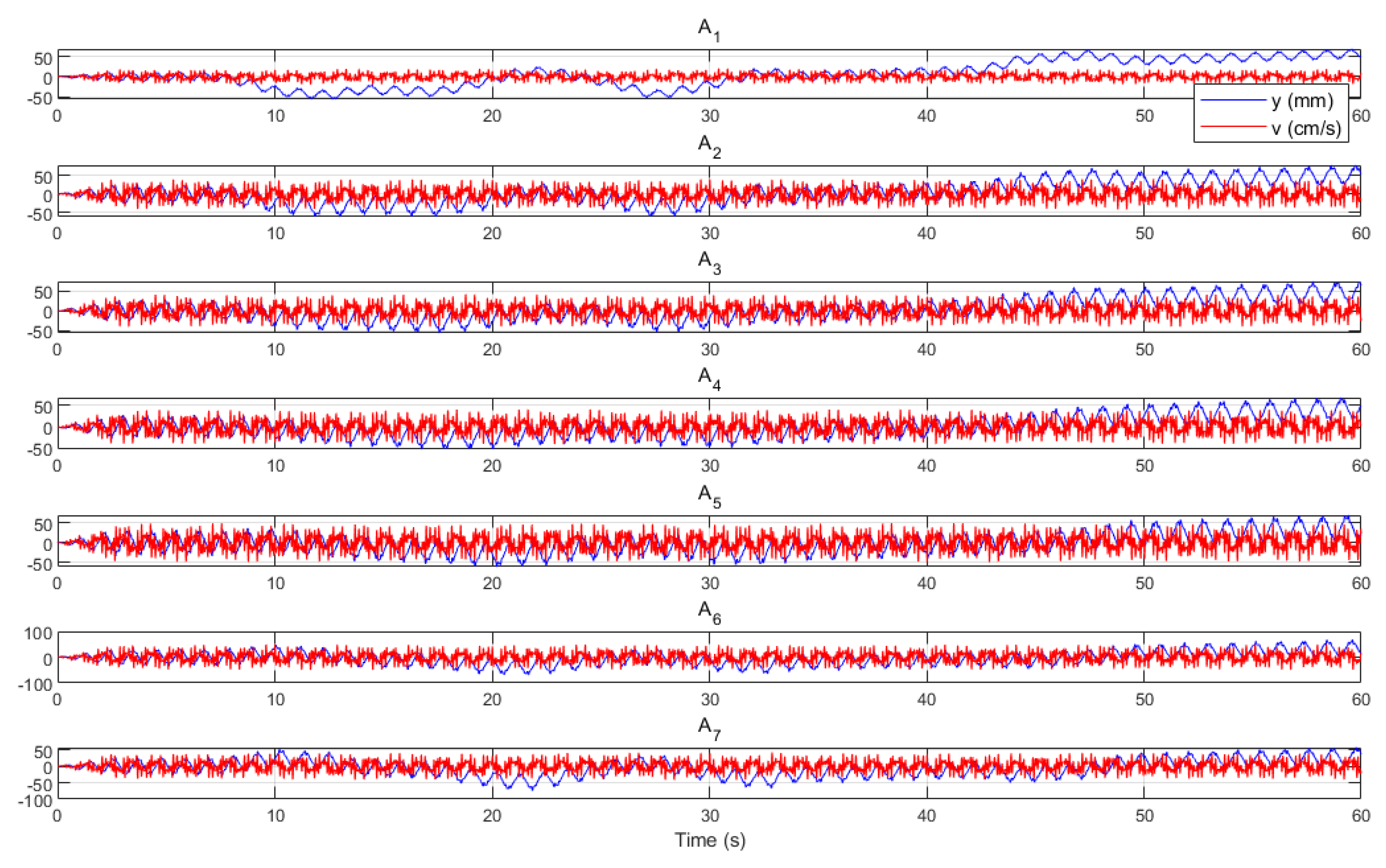
Figure 8.
Decomposition of the position data into the linear oscillations and the gross motion.
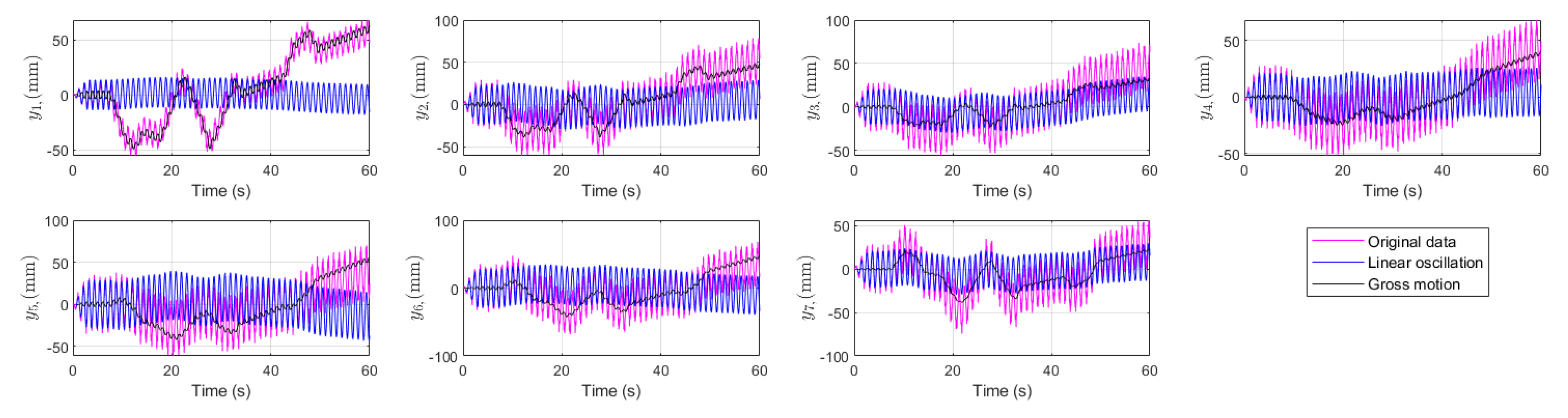
Figure 9.
Reconstruction of the data with the main modes and the reconstruction error.
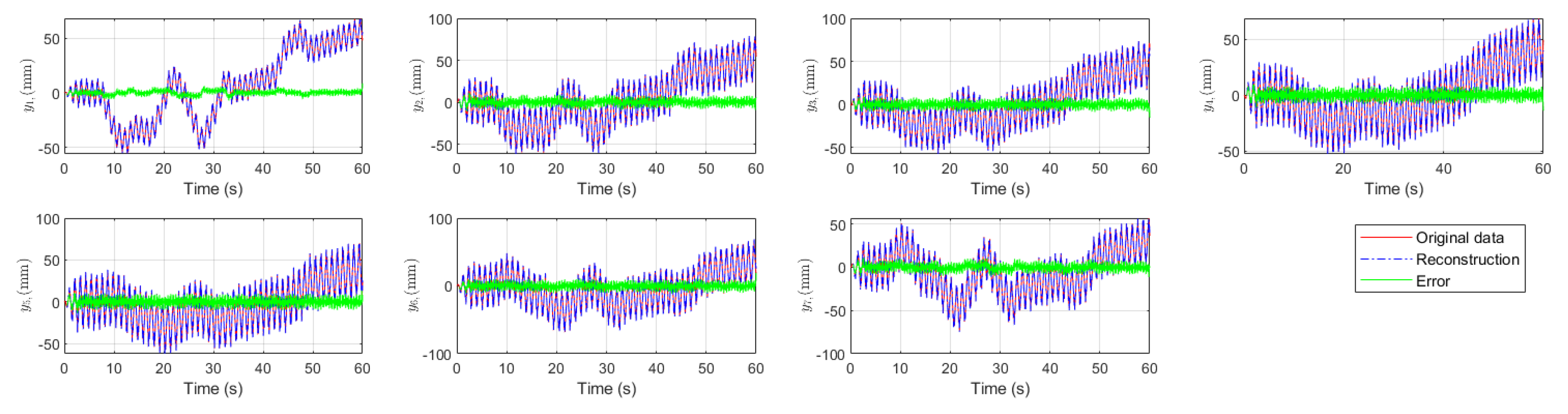
Figure 10.
Results of the CDE DMD gross motion prediction (training scenario).
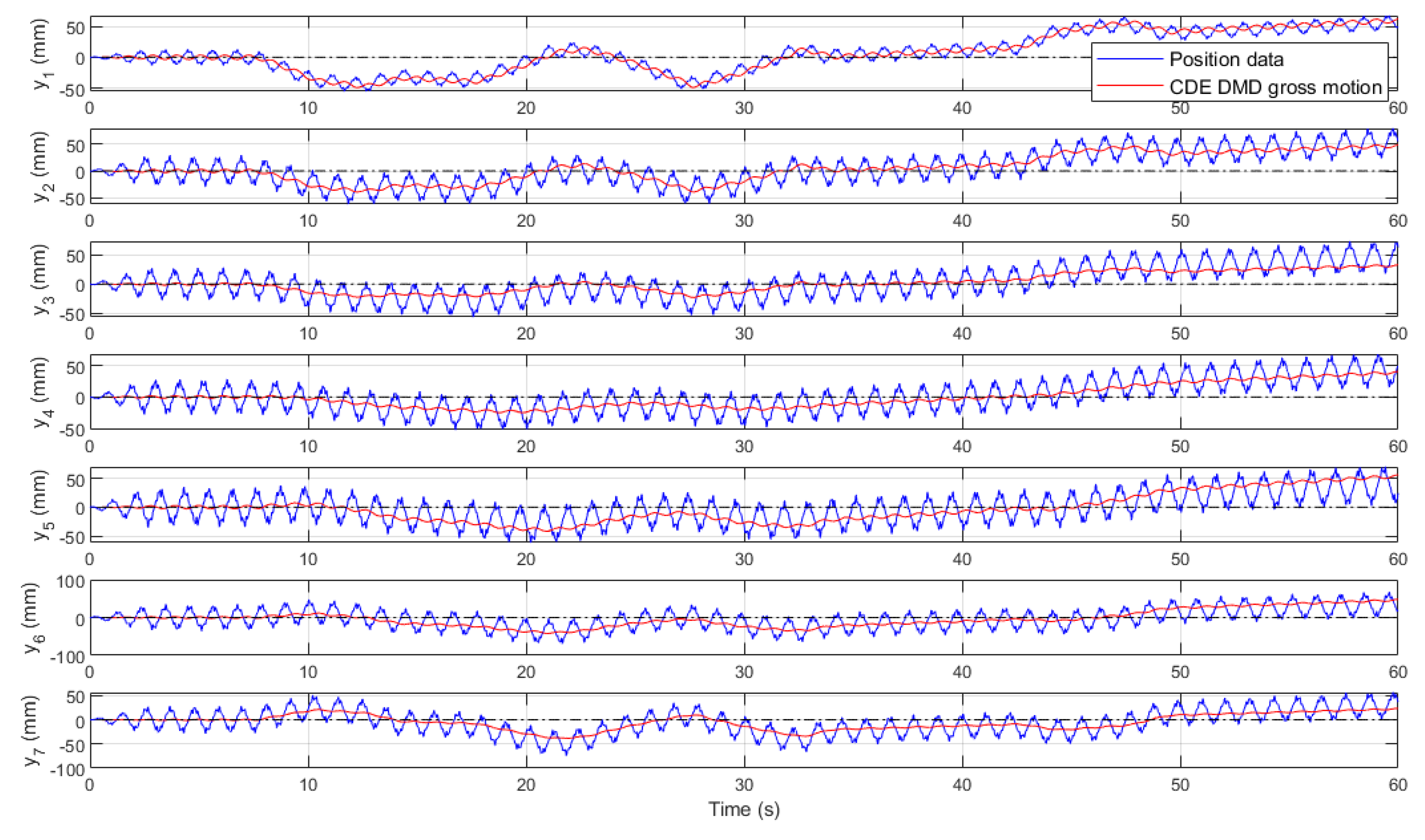
Figure 11.
Arbitrary input in the unseen scenario.
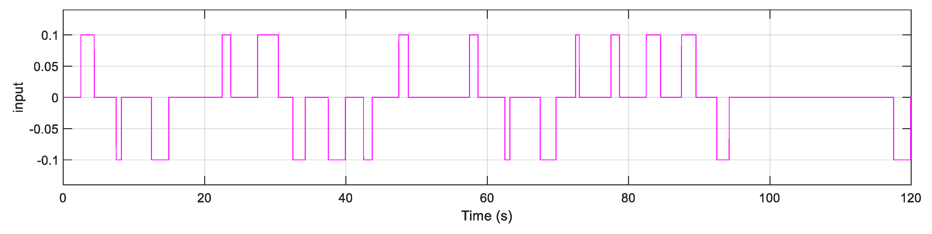
Figure 12.
Results of the CDE DMD gross motion prediction for the unseen scenario.
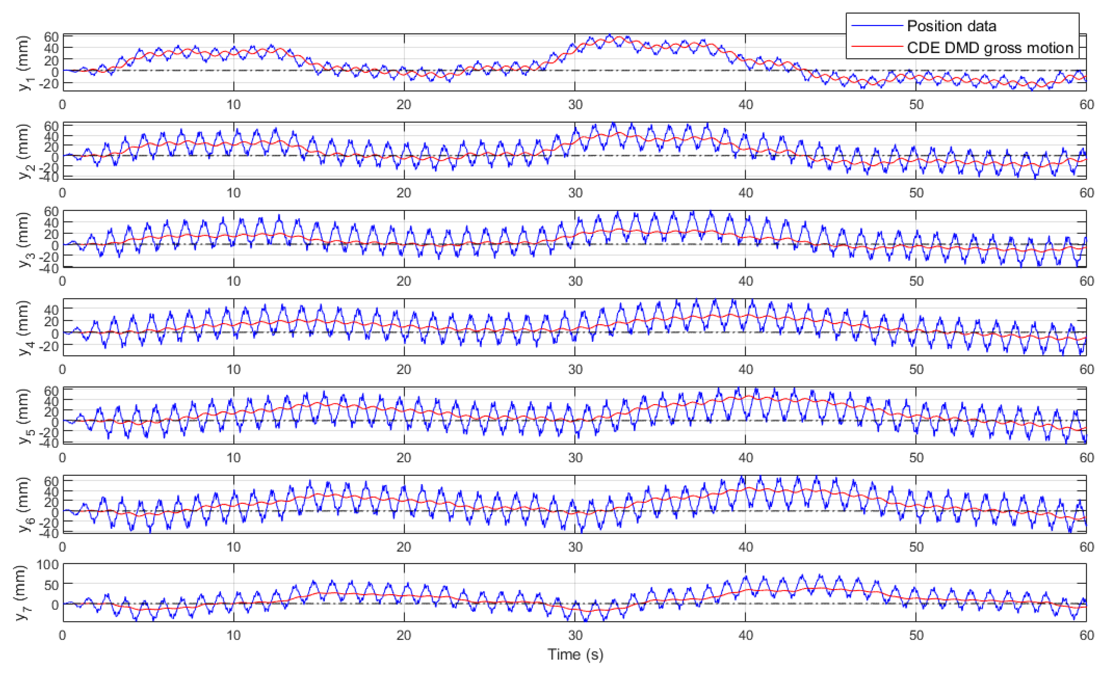
Figure 13.
A closed-loop scenario of CDE DMD directional control for a nonzero initial orientation.
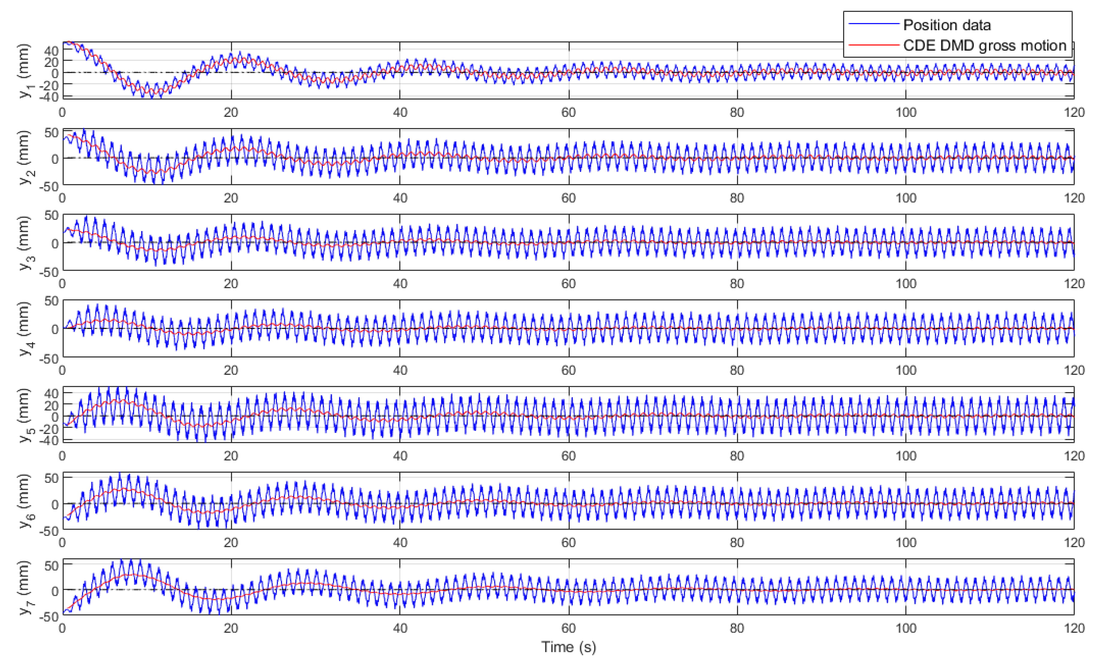
Figure 14.
A closed-loop scenario with an initial distance dislocation.
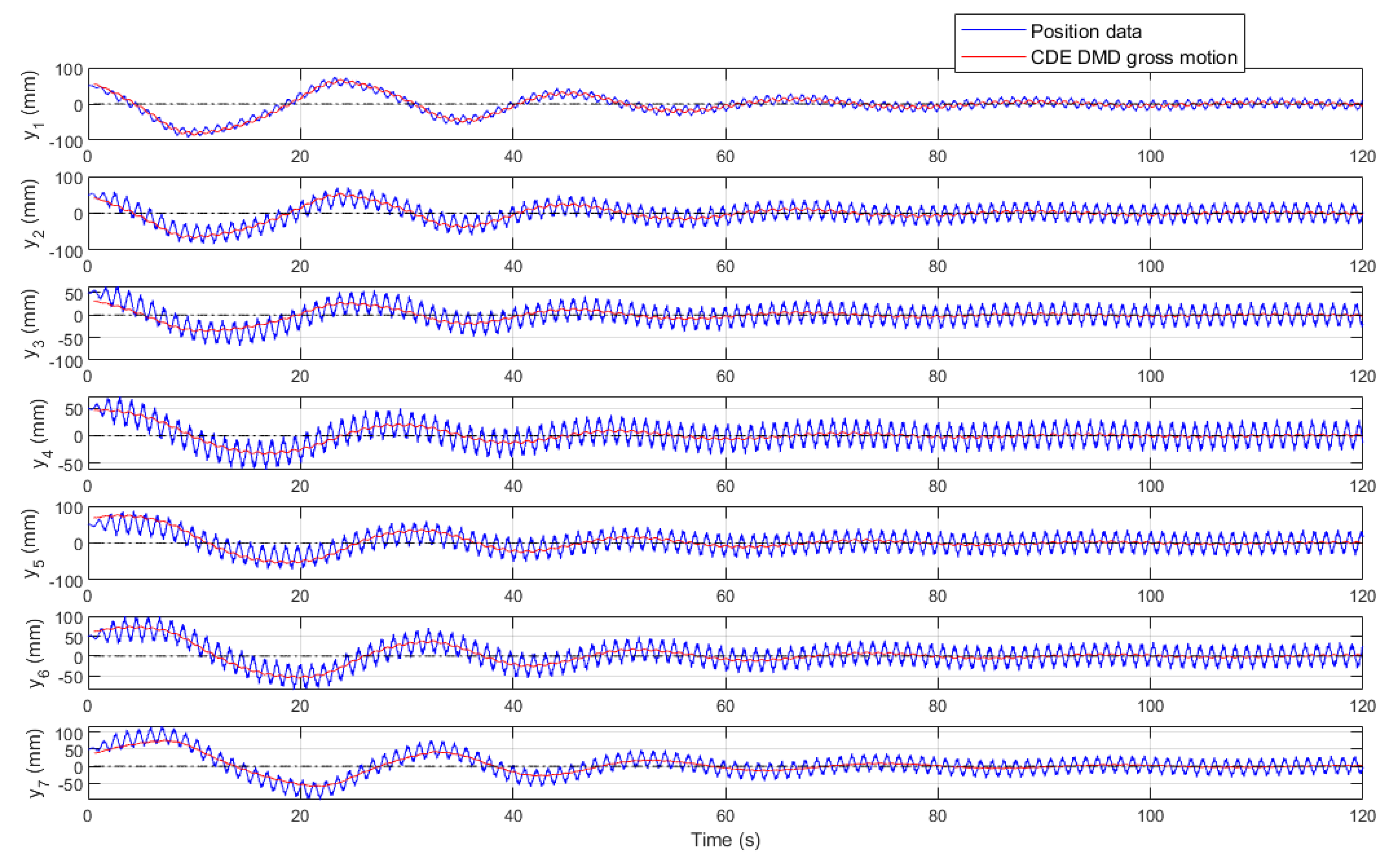
Figure 15.
Pneumatic circuit for actuation of the soft robot.
Disclaimer/Publisher’s Note: The statements, opinions and data contained in all publications are solely those of the individual author(s) and contributor(s) and not of MDPI and/or the editor(s). MDPI and/or the editor(s) disclaim responsibility for any injury to people or property resulting from any ideas, methods, instructions or products referred to in the content. |
© 2025 by the authors. Licensee MDPI, Basel, Switzerland. This article is an open access article distributed under the terms and conditions of the Creative Commons Attribution (CC BY) license (http://creativecommons.org/licenses/by/4.0/).
Copyright: This open access article is published under a Creative Commons CC BY 4.0 license, which permit the free download, distribution, and reuse, provided that the author and preprint are cited in any reuse.


