Submitted:
23 July 2025
Posted:
24 July 2025
You are already at the latest version
Abstract
This study introduces the Normalized Difference Gamma Ray Index (NDGRI), a novel spectral composite derived from Sentinel 2 imagery for mapping elevated natural gamma radiation in semi arid and arid basins. We hypothesized that water‐sensitive spectral indices correlate with gamma‐ray hotspots in arid regions of Mongolia, where natural radionuclide distribution is influenced by hydrological processes. Leveraging historical car-borne gamma spectrometry data collected in 2008 across the Sainshand and Zuunbayan uranium project areas, we evaluated twelve spectral bands and five established moisture-sensitive indices against radiation heatmaps in Naarst and Zuunbayan. Using Pearson and Spearman correlations alongside two percentile based overlap metrics, indices were weighted to yield a composite performance score. The best performing indices (MI - Moisture Index and NDSII_1 - Normalized Difference Snow and Ice Index) guided the derivation of ten new ND constructs incorporating SWIR bands (B11, B12) and visible bands (B4, B8A). The top performer, NDGRI = (B4–B12)/(B4 + B12) achieved a precision of 62.8% for detecting high gamma‐radiation areas and outperformed benchmarks of other indices. We established climatological screening criteria to ensure NDGRI reliability. Validation at two independent sites (Erdene, Khuvsgul) using 2008 airborne gamma ray heatmaps yielded 68.1% and 45.4% overlap, respectively. Our results demonstrate that NDGRI effectively delineates gamma radiation hotspots where moisture controlled spectral contrasts prevail. The index’s stringent acquisition constraints, however, limit temporal availability of usable scenes. NDGRI offers a rapid, cost effective remote sensing tool to prioritize ground surveys in uranium prospective basins and may be adapted for other radiometric applications in semi arid and arid regions.
Keywords:
normalized difference gamma-ray index (NDGRI)
; Sentinel-2 remote sensing
; uranium exploration
1. Introduction
Mongolia’s uranium potential has been systematically investigated since the 1950s, with Soviet led airborne radiometric surveys evolving into detailed car-borne spectrometry and geochemical investigations by the 1970s–1980s. Over 30 technical reports (1970–1990) documented uranium occurrences, later made public via Mongolia’s Mineral Resources Authority (MRAM) in 2006 [1]. Post-1990, international consortia revitalized exploration, leveraging Mongolia’s geotectonic division into northern (Precambrian–Paleozoic) and southern (Paleozoic–Mesozoic) provinces along the Main Mongolian Lineament, a key suture in the Central Asian Orogenic Belt [1,2]. Uranium mineralization models, notably by Mirnov [3] and Rutherford [4], highlight diverse genetic settings: from magmatic-hosted U⁴⁺ in granites/rhyolites to redox-controlled deposits in Mesozoic–Cenozoic basins.
Geological literature dating back to the 1970s consistently divides Mongolia into two primary geotectonic provinces: a northern and a southern domain [5]. These are delineated by the Main Mongolian Lineament, a major structural boundary that separates Precambrian and Early Paleozoic formations of the northern region from the predominantly Paleozoic to Mesozoic lithological assemblages in the south. This lineament represents a significant tectonic suture and has played a pivotal role in the evolution of the Central Asian Orogenic Belt. Its structural and lithostratigraphic significance forms a fundamental framework for interpreting regional tectonics, magmatism, and mineralization patterns across Mongolia.
Both Mironov [3] and Rutherford [4] categorize Mongolian uranium occurrences based on genetic setting and host environments, though they emphasize different geological controls. Mironov’s classification spans seven types, from fluorine–molybdenum–uranium mineralization in Late Mesozoic volcano-tectonic settings, to uranium in terrigenous Mesozoic and Cenozoic depressions, coal-bearing strata, and weathered leucogranites—emphasizing both magmatic and sedimentary processes across temporal and lithological contexts [3]. Rutherford [4], meanwhile, introduces a threefold model: Type 1 includes uranium in intrusive contacts and shear zones within granitic skarn and pegmatite systems of cratonic terrains—linked to Sn, Th, REE, and other critical elements but deemed economically marginal. Type 2 covers volcanic–intrusive zones of intracratonic settings with modest potential, while Type 3 highlights sediment-hosted uranium in Cretaceous to Neogene rift basins, influenced by redox dynamics and groundwater chemistry. Together, these frameworks underscore Mongolia’s diverse uranium metallogeny, from primary magmatic sources to secondary mobilization in continental sedimentary basins. This layout highlights how Mironov provides a broader spectrum of genetic types—especially those linked to sedimentary environments—while Rutherford zeroes in on tectonic and redox-controlled systems with emphasis on exploration viability [3,4].
Previous efforts to map gamma-radiation anomalies have employed a variety of remote-sensing and geophysical techniques. Ondieki et al. demonstrated that supervised classification of Landsat-8 surface reflectance into vegetation and soil/rock classes could predict thorium-rich outcrops at Mrima Hill, Kenya, with approximately 90 % overall accuracywhen validated against field gamma-dose measurements [6]. Saepuloh et al. extended this approach by using Sentinel-2 band-ratio composites and a red-edge vegetation stress index (REVI) to identify uranium-bearing hydrothermal alteration in Sulawesi, Indonesia, finding that areas of anomalous REVI values corresponded closely with elevated uranium assays [7]. In Egypt’s Eastern Desert, Assran et al. fused Sentinel-2 false-color composites, principal component analysis, and SWIR band ratios with airborne gamma-spectrometry (K, eU, eTh) to produce integrated radiometric anomaly maps that aligned strongly with known uranium mineralization [8]. Similarly, Ahmed et al. combined eU/eTh ratio maps from airborne data with Landsat and Sentinel alteration signatures to trace uranium migration pathways in the Duwi and Quseir formations, achieving high spatial concordance between spectral alteration and radiometric hotspots [9].
Remote sensing offers a powerful complement to field based gamma surveys, especially in arid terrains where sparse vegetation and low ambient moisture minimize spectral interference. Our central hypothesis is that moisture sensitive composite indices, when applied to Sentinel 2 Level 2A imagery acquired under strict climatological constraints, will spatially co locate with zones of naturally elevated gamma radiation. This alignment reflects the oxidative mobilization of uranium and its moisture driven transport pathways. By quantitatively evaluating existing indices and developing a new Normalized Difference Gamma Ray Index (NDGRI), we address a critical gap in exploration technology for semi-arid basinal environments.
The primary objective of this study was to develop a purely remote-sensing approach that can precede, and sharply narrow, the scope of traditional uranium exploration in arid and semi-arid basins. Conventional workflows rely on costly airborne and ground spectrometry campaigns, followed by even more expensive drilling and geochemical assays to confirm uranium occurrence. By introducing the NDGRI, computed solely from Sentinel-2 imagery, we aim to delineate prospective uranium-bearing zones without any initial field deployment. This pre-screening step can guide and optimize the placement of airborne surveys, ground radiometric traverses, and drill exploratory holes, thereby reducing the overall survey footprint and delivering substantial economic savings. NDGRI serves as an efficient filter—directing expensive follow-up operations to areas most likely to host elevated gamma radiation and, by proxy, uranium mineralization.
2. Materials and Methods
2.1. Test Areas
For the gamma-radiation analysis, two areas in Dornogovi Province were selected: Naarst (110.55° E–110.65° E, 44.86° N–45.02° N, WGS 84/UTM Zone 49N), hereafter referred to as Area 1, and Zuunbayan (110.16° E–110.34° E, 44.17° N–44.42° N, WGS 84/UTM Zone 49N), hereafter referred to as Area 2 (Figure 1). Raster format heatmaps for these sites, acquired via the car-borne gamma spectrometer survey detailed in Section 2.4, were rendered using three spectral bands (red, green, and blue). To improve comparability, the heatmaps were subjected to two preprocessing workflows prior to analysis.
2.Organization of the Database of Anomalies and Zones
As baseline material, for this paper and other purposes the dataset was compiled from selected Soviet-era geological reports, text excerpts, and scanned map materials, obtained from the MRAM under the official terms in effect between June and September 2006. The acquired materials were integrated into a purpose-built database on uranium and radioactive anomalies across Mongolia, with initial data structuring conducted during 2006–2007. Subsequent revisions and data corrections were implemented in 2012 to enhance spatial accuracy and attribute consistency, ensuring the dataset’s reliability for geospatial analysis and remote sensing validation [11].
A total of 22 Soviet-era reports (No. 2447, 2462, 5251, 2411, 2448, 2449, 2427, 2419, 2520, 2452, 2426, 2442, 2437, 2414, 2453, 2455, 2428, 2429, 2432, 4289, 4358, and 4454) were reviewed and integrated into an Excel-based anomaly and zone database according to the MRAM referencing system [11].
2.3. Regional Geology of Dornogovi and Areas of Interest (Naarst and Zuunbayan)
The regional geology of Dornogovi Province was established through a synthesis of Soviet-era geological surveys [11,12], the national geologic map of Mongolia and its accompanying documentation, as well as direct field observations and satellite imagery analysis [13]. This integrated framework provided a foundational geological context, enabling the identification and interpretation of structurally favourable settings and lithological units relevant to uranium mineralization [13]. It also supported the remote sensing–based delineation of anomalous zones, forming a geospatial baseline for further spectral and radiometric investigations.
The two localities investigated in this study, Naarst and Zuunbayan, are aligned along a NE–SW-trending corridor approximately 75 km in length and lie within the Upper Cretaceous Bainshiren Suite (K2bš). This formation, dated to approximately 98–83 Ma (or alternatively 93–80 Ma), comprises grey sandstones, gravel-rich horizons, and interbedded red and grey clays. The area is structurally complex, marked by uplifted Paleozoic basement blocks and active tectonism, which together foster the development of uranium and associated radioactive anomalies (Figure 2).
The Naarst area has undergone extensive uranium exploration, initially by Soviet teams between 1978 and 1981, resulting in over 250 drill holes, and subsequently through additional boreholes drilled between 2006 and 2009 by Western companies. These efforts were triggered by the detection of uranium anomalies in the late 1970s. The region's current surface geology, dominated by sand, gravel, and locally derived sandstone, reflects its sedimentary context within the Cenomanian–Santonian formations (K2ss2 and K2bš) [11]. Despite post-drilling contamination from radioactive drilling mud pits that hindered auto-gamma surveys, spectrometric data revealed elevated uranium values in both grey (reduction-favoring) and yellowish-to-brownish sandstones. Notably, uranium mineralization appears to concentrate near the convergence of two paleo drainage systems beneath a thin Quaternary cover—features clearly distinguishable via satellite imagery. The area is structurally complex, with active tectonism producing a network of crosscut faults and generating discrete blocks measuring approximately 500–700 × 100–150 m. However, recent investigations have not confirmed the presence of a coherent ore body amenable to in situ leaching [15]. Although the anomalies trace similar structural trends, mineralized intersections occur at variable or excessive depths, in some cases exceeding 400 meters.
The Zuunbayan area, delineated within the Upper Cretaceous Bainshiren Suite (K2bš), exhibits high uranium potential as evidenced by drilling conducted between 2008 and 2009. Although initial gamma anomalies were identified in the early 1980s, systematic uranium exploration commenced only after 2006 [14]. Spanning approximately 22 km in length and 4–7 km in width, the zone functions as a natural groundwater collector—confirmed by satellite imagery—and is marked by significant subsurface hydrodynamics. Drilling operations frequently triggered spontaneous groundwater upflows, occasionally requiring relocation of rigs to prevent instability. Despite minimal vegetation, the area's wetland-like conditions and surface instability from unconsolidated sediments rendered access and conventional geological mapping particularly difficult. Nonetheless, auto-gamma surveys corroborated earlier Soviet data, and oxidized brown sandstone outcrops were successfully identified. Subsurface investigations revealed multiple uranium-enriched intersections, typically at depths between 220 and 340 meters, with concentrations exceeding 200 ppm [15], suggesting promising potential for the identification of an economically viable ore body in future detailed exploration.
2.4. Car-Borne Gamma Spectrometer Survey
A car-borne gamma spectrometry survey was conducted in 2008 across the Sainshand and Zuunbayan uranium project areas using the RS-700 system [16], a high-resolution, 1024-channel gamma-ray spectrometer developed by Radiation Solutions Inc. (Canada). The system was equipped with a 4-liter NaI (Tl) detector mounted on a Toyota Land Cruiser 4×4, with data acquisition and control managed via a Panasonic Toughbook laptop. The RS-700 operates across an energy range of 20 keV to 3 MeV and is capable of handling count rates up to 250,000 cps with less than 20% dead time, ensuring high spectral fidelity even under elevated radiation conditions. Background levels typically remain below 100 cps, while elevated readings in the several hundred cps range may indicate natural enrichment; values exceeding 1,000 cps are considered anomalous and may suggest contamination or unexpected radioactive sources. The system’s advanced digital signal processing and automatic gain stabilization enable reliable field performance without the need for radioactive calibration sources [16].
Figure 3 depicts Gamma-count distribution in the Naarst and Zuunbayan study areas over predominantly sandy-gravel terrain: readings > 300 cps are shown in red, 200–300 cps in yellow, 100–200 cps in green, and < 100 cps in blue.
2.4. Methodology
As illustrated in Figure 4, our workflow began with the hypothesis that pixels exhibiting high values in water sensitive composite indices would partially coincide with zones of elevated gamma radiation in semi-arid basinal environments, reflecting the natural distribution of radioactive elements and their mobilization by episodic moisture. To test this, we acquired Level 2A Sentinel 2 imagery and overlaid it on raster heatmaps from a car-borne gamma spectrometer survey of two study areas (Naarst and Zuunbayan). We converted the RGB heatmaps to grayscale using a custom formula. We also applied ISO Cluster classification to the RGB heatmaps before reclassifying the resulting clusters into three gamma radiation classes. A suite of established and newly derived normalized difference composite indices were evaluated against these classes using Pearson and Spearman correlations, two percentile based overlap metrics, and confusion matrix–derived precision, recall, F1, and overall accuracy. Finally, we combined these metrics into a weighted scoring system to rank and select the top performing indices for mapping high–gamma radiation hotspots.
To enable direct statistical comparison between the multi-band gamma-ray heatmaps and the single-band composite indices, each RGB heatmap raster was converted into a single-band (grayscale) raster. This transformation collapses the three-color channels into a single intensity value per pixel. The resulting grayscale rasters facilitate scalable data handling, streamline subsequent geospatial processing, and ensure compatibility with one-band index evaluation workflows. Standard RGB to grayscale conversion methods include [17]:
- Luminosity Method – This approach accounts for the human eye’s varying sensitivity to different colors by computing the grayscale value as a weighted average of the R, G, and B channels:
- Arithmetic Mean Method – A simpler technique that calculates the grayscale value as the unweighted average of all three channels:where , , and are the red, green, and blue band values, respectively [17].
However, because our heatmaps’ hotspots are characterized by extremely high red-band values (with green and blue near zero), we adopted a customized formula that accentuates the red channel and de-emphasizes the others [17]:
Unlike conventional formulas, whose weights sum to unity to preserve overall brightness, our weights sum to 0.7 in order to maximize contrast between high–gamma-radiation regions and the surrounding background. This specific weighting provided clearer delineation of radiation hotspots and yielded more reliable pixel values for subsequent correlation analyses (Figure 5.).
2.5. ISO-Cluster Classification
The original heatmaps were also processed using the ISO-Cluster classifier in ArcGIS Pro, an unsupervised classification method based on the K-means clustering algorithm. Unlike supervised approaches, ISO-Cluster does not require pre-defined training samples. Instead, it automatically partitions pixels into groups according to their spectral similarity. We set the maximum number of clusters to ten, allowing the algorithm to iteratively assign each pixel to the cluster whose mean spectrum most closely matches its own and then update cluster centroids until convergence [18]. This procedure yields a raster in which each pixel is labeled by its spectral class, facilitating the isolation of gamma-ray anomaly zones for subsequent analysis.
Following ISO-Cluster classification, Area 2 yielded ten spectral classes (values 0–9), with class 9 corresponding to the highest gamma-radiation levels and class 0 to the lowest. In Area 1, nine classes (0–8) were produced, where class 8 represented the most intense gamma-radiation zones and class 0 the background. Because the original heatmaps exhibited three distinct gamma-radiation regimes, high (>300 cps), medium/low (200–300 cps), and negligible (<200 cps), we reclassified the ISO-Cluster outputs into three consolidated classes (Figure 6.):
- Class 2 (High gamma radiation): Area 1’s class 8; Area 2’s class 9
- Class 1 (Medium/Low gamma radiation): Area 1’s class 7; Area 2’s classes 8 and 7
- Class 0 (Negligible gamma radiation): Area 1’s classes 1–6; Area 2’s classes 1–6
3. Results
3.1. Composite Index Evaluation
Sentinel 2 Level 2A imagery, acquired on 20 September 2022 under exceptionally favorable conditions (0 % cloud cover, 0.007 % vegetation cover, 0 % snow and ice cover and mean water vapor content of 0.77 g/cm²) was used for composite index evaluation. Ambient surface temperatures during acquisition ranged from 6.3 °C to 19.7 °C, and no rainfall occurred on the acquisition date or in the preceding two weeks.
Based on our initial hypothesis, we evaluated all spectral bands of the Sentinel 2 scene as well as a suite of composite indices sensitive to water-related surface changes. First, each index was visually compared against the spatial distribution of gamma radiation hotspots on the heatmaps, and indices exhibiting substantial mismatches were excluded. Next, we conducted a detailed analysis of spectral bands B1 through B12 and the following composite indices: MI - Moisture Index ((B8A - B11) / (B8A + B11)), NDSI - Normalized Difference Snow Index ((B3 - B11) / (B3 + B11)), NDWI - Normalized Difference Water Index ((B3 - B8) / (B3 + B8)) [19], WRI - Water Ration Index ((B3 + B04) / (B08 + B11)) [20] and NDSII_1 - Normalized Difference Snow and Ice Index ((B4 - B11) / (B4 + B11)) [21].
Correlations between each index and the classified gamma radiation zones were quantified using:
- 4.
- Pearson’s correlation coefficient
- 5.
- Spearman’s rank correlation coefficient
- 6.
- Two percentile based comparisons. This section may be divided by subheadings. It should provide a concise and precise description of the experimental results, their interpretation, as well as the experimental conclusions that can be drawn.
3.2. Pearson and Spearman Correlation
In statistics, the Pearson and Spearman coefficients quantify the correlation between two datasets. Pearson’s coefficient evaluates the relationship as a linear function, whereas Spearman’s assesses it as a monotonic function. Both coefficients range from –1 to 1, where 1 denotes a perfect positive correlation, –1 a perfect negative correlation, and 0 no correlation at all. Because they summarize correlation across entire datasets, these metrics are only partially suited for evaluating the relationship between composite indices and gamma radiation—our hypothesis concerns the co occurrence of hotspots (i.e., pixels with both high index values and high gamma readings), not the overall raster. Consequently, we do not expect extremely high Pearson or Spearman values; nevertheless, they remain valuable evaluation parameters, with their limitations addressed by the subsequent percentile based comparisons [22].
3.3. Percentile-Based Comparisons
Percentiles are a statistical measure that partition a dataset into 100 equal segments, where each percentile denotes the value below which a specified percentage of observations lie. This approach provides a nuanced view of the data distribution, its concentration, and the relative positioning of particular values within the overall dataset.
We designed two percentile based comparisons to evaluate the “predictive power” of each composite index, that is the extent to which the pixels with the highest index values (hotspots) coincide with areas of elevated gamma radiation [23].
In the first comparison, the 95th percentile of each composite index was calculated, and all pixel values below this threshold were discarded, leaving the top 5 % of pixels (those with the highest index values) designated as composite hotspots. The 70th percentile of the grayscale gamma-radiation heatmap was then computed, and, by the same criterion, only pixels exceeding this threshold (the top 30 % in terms of radiation) were retained. Finally, we determined the proportion of composite-hotspot pixels (above the 95th percentile) that overlapped with the heatmap pixels above the 70th percentile.
The second comparison assessed the fraction of the top 5 % of composite-index pixels (those above the 95th percentile) that fell within the Class 2 polygon of the ISO-Cluster classified heatmap, which corresponds to the highest gamma-radiation zones. The outcomes of both comparisons were expressed as values between 0 and 1 (or 0% – 100%), indicating the predictive alignment of the composite indices with elevated gamma-radiation areas.
3.4. Interpretation of Evaluation Results
In the first step, we calculated the five comparison metrics for each individual spectral band and established composite indices, the results are presented in Table 1 below. We then aggregated these metrics into a single composite score, assigning a greater weight (70 %) to the parameters derived from Area 2—owing to its more naturally distributed radiation pattern compared to Area 1 (30 %), as discussed earlier. The composite score E (expressed on a 0–1 scale, or 0%–100%) was computed using:
In this formula, PC denotes the Pearson correlation coefficient, SC the Spearman correlation coefficient, P1 the result of the first percentile based comparison, and P2 that of the second. Subscript “1” refers to metrics from Area 1 and subscript “2” to those from Area 2. The final composite scores are listed in Table 1.
Analysis of the results showed markedly better performance in Area 2 compared to Area 1, as expected, since the gamma radiation distribution in Area 2 is naturally controlled, whereas in Area 1 it is influenced by anthropogenic factors. The composite indices MI and NDSII_1 achieved the highest scores, exhibiting the strongest correspondence between their hotspots and zones of elevated gamma radiation. Both indices are defined using normalized difference (ND) formulas and incorporate band B11 (SWIR 1, ~1610 nm) in the denominator, a wavelength at which water absorption is particularly strong.
Moreover, in Area 2 we observed negative Pearson and Spearman correlation values for band B11, as well as for band B12 (SWIR 2, ~2190 nm), deviating from the behavior of other bands (see Table 1). Band B12 also experiences strong water absorption. Consequently, we formulated new theoretical indices, still using ND constructs that employ B11, B12, or both as the subtractive term. Both MI and NDSII_1 include band B4 (red, ~665 nm), another water absorptive wavelength, and band B8A (narrow NIR, ~865 nm), which is highly reflective in healthy vegetation. For the new formulas’ denominators, we also experimented with other visible and NIR bands, motivated by the observed decline in Pearson correlation and overall composite score E in Area 2 as band wavelength increases (see Table 1).
The newly derived indices were evaluated in both areas using the same methodology, and their results (ranked from best to worst) are presented in Table 2. These tailored, theoretically grounded composites have met expectations by outperforming the established indices under the specific conditions of gamma radiation comparison.
Subsequently, the ten composites with the highest evaluation scores were classified and are henceforth referred to by their ordinal numbers (Figure 8).
3.5. Classification of Top-Performing Composites
The ten highest scoring composites were classified into three categories: Class 2 (high gamma radiation zones), Class 1 (medium and low gamma radiation zones), and Class 0 (negligible gamma radiation zones). The first step was to determine the pixel value thresholds that would delineate these classes.
Common image segmentation algorithms isolate objects from the background by identifying a critical grayscale threshold. In bimodal images, the histogram exhibits two dominant peaks—one corresponding to object pixels and the other to background pixels—separated by a pronounced valley. The optimal threshold is placed at this minimum to minimize misclassification of pixels between the two groups [24].
We implemented a multi class extension of this approach as follows:
- Each composite was overlaid with the ISO Cluster classification of Area 2, since Area 2 exhibits a natural gamma radiation distribution (Figure 9.).
- Three histograms were generated, each representing the distribution of composite pixel values within the polygon for one of the three heatmap classes.
- The class boundaries for the composite were chosen at the intersections of these overlaid histograms, ensuring that within each composite class the maximum number of pixels coincided with the corresponding heatmap class.
The threshold, or critical value, between each pair of composite classes was set at the intersection of the overlaid histograms. These histograms represent the distribution of composite pixel values within the polygons of the classified heatmap classes. Our goal was to position the boundaries so that, for each composite class, the greatest possible number of pixels fell within the corresponding heatmap class. In ideal conditions, the histogram intersection would lie in the valley between two dominant peaks, although that was not precisely the case here, the desired outcome was still achieved (Figure 10.).
The exact pixel values defining the class boundaries for each composite are listed in Table 3. After converting these values into percentiles, we found that the boundary between Class 2 and Class 1 for all composites falls at approximately the 95th percentile, while the boundary between Class 1 and Class 0 is around the 88th percentile. Figure 11. shows the classified heatmap alongside the composites for Area 2.
Subsequently, the composites in Area 1 were classified using the exact pixel-boundary values determined for each class (Figure 12).
3.6. Assessment of Composite Predictive Power
To assess each composite’s predictive power, we compared its three classes (2, 1, and 0) against the three classes of the ISO-Cluster–classified heatmaps for both Area 2 and Area 1. For each area, we first built a confusion matrix in which the reference (target) labels were the classes from the gamma-radiation heatmap, and the predicted labels came from the classified composite. For each class we then computed [18]:
- True Positive area (TP): the overlap between the predicted class polygon and the reference class polygon—i.e., the area correctly predicted.
- False Positive area (FP): the portion of the predicted class polygon that does not overlap the reference polygon—i.e., over prediction, or “commission error.”
- False Negative area (FN): the portion of the reference class polygon that does not overlap the predicted polygon—i.e., under prediction, or “omission error.”
Using TP, FP, and FN, we derived the following metrics for each class:
-
Precision: (5)Precision quantifies the accuracy of predicted areas: the proportion of the predicted class area that is correct. A high precision indicates that most of the predicted region overlaps the reference.
-
Recall: R (6)Recall measures completeness: the proportion of the reference class area that was correctly predicted. A high recall means that most of the true class area was captured, indicating few omissions.
-
(7)The F1 score is the harmonic mean of precision and recall, providing a single balance metric between over prediction and under prediction.
-
Overall Accuracy: (8)Overall Accuracy (OA) is defined as the ratio of the sum of true positive areas across all classes to the total area of all cases across all classes. This metric provides a general measure of classification performance, where a value of 1 indicates perfect agreement between the predicted and reference data.
To quantify the predictive power of each composite index, we computed a score G using the formula:
Here, F2, F1 and F0 are the F₁ scores for classes 2, 1, and 0 respectively; P2, P1 and P0 are their corresponding precision values; and OA is the overall accuracy. The subscript “1” denotes metrics for Area 1, and “2” for Area 2.
When weighting the parameters, we allocated the highest weight (0.6) to class 2, 0.1 to each of classes 1 and 0, and 0.2 to overall accuracy. This is because class 2 represents the high gamma-radiation zone, and the accuracy of predicting this zone is paramount, since the objective is to successfully predict areas with elevated gamma-radiation based on the composites. At the area level, Area 2 was given a weight of 0.7 and Area 1 a weight of 0.3, reflecting the fact that gamma-radiation in Area 2 follows a natural distribution, whereas in Area 1 it is anthropogenically influenced. Moreover, because anthropogenic factors in Area 1 cause class 2 to cover an unnaturally large extent recall was very poor. This also impacts the F1 score values, and because precision is far more critical than recall for predicting gamma-radiation zones, precision was used as a parameter in the formula. The resulting score was then multiplied by 10 to produce a 0–10 scale (Table 4).
3.7. Validation at Other Explored Areas
We evaluated NDGRI in two additional test sites in Mongolia, both in Dornogovi Province. The first site lies near Erdene (110.99°E-111.35°E, 44.22°N-44.84°N,WGS 84 /UTM Zone 49N), and the second near Khuvsgul (109.51°E-110.35°E, 43.53°N-43.67°N, WGS 84 / UTM Zone 49N). Sentinel-2 scenes were selected according to the climatological limitations, the Erdene image was acquired on 2023-08-19, and the Khuvsgul image on 2023-07-30. For each site, we identified all pixels with NDGRI values between –0.129 and –0.040 (classes 1 and 2) and calculated the percentage of those pixels overlapping high–gamma-radiation areas delineated from airborne gamma-spectrometry heatmaps. The heatmaps derive from an airborne gamma-ray survey conducted in 2008 by GEOSAN LLC over the Sainshand uranium project area, flown in a Cessna 208B fixed-wing aircraft equipped with a dual-detector radiometric system comprising two Radiation Solutions RSX-4 spectrometers [25]. Each sensor contains four 4-liter NaI (Tl) crystals (16 L per unit, 32 L total), and employed a 1024-channel digital MCA spanning approximately 12 keV to 3 MeV with an energy resolution better than 8.5 % FWHM at 662 keV. Each crystal sustained count rates up to 250,000 cps with minimal dead time, ensuring high fidelity even over strongly radioactive targets. Automatic multi-peak gain stabilization—referencing natural isotopes of K, Th, and U—maintained peak drift below 0.5 % without the need for onboard calibration sources, although daily pre- and post-flight thorium checks were performed at a fixed airfield position. Data were recorded every second (approximately 75 m along-track at a nominal speed of 75 m/s) as both full 256-channel spectra and five standard energy-window count rates (total count, K-40, Bi-214, Tl-208, and cosmic), then subjected to dead-time correction, background subtraction (aircraft, cosmic, and radon), NASVD noise reduction, Compton stripping, and height-attenuation correction to produce calibrated eU, eTh, K, and total-count data suitable for geological mapping [26]. The heatmaps were classified in ArcGIS Pro using an ISO Cluster (K-means) classifier and then reclassified into two polygons (high-radiation vs. background). In the Erdene site (Figure 13.), 68.1% of class 1–2 pixels coincided with the high-radiation polygon, whereas in the Khuvsgul site (Figure 14.) the overlap was 45.4%.
4. Discussion
The ranking of composites in our evaluation clearly highlights the superior performance of the newly derived indices over established moisture-sensitive metrics. Composite 7 achieved the highest composite score (6.09), closely followed by Composite 10 (5.99), Composite 2 (5.92), Composite 3 (5.88), and Composite 1 (5.84). By contrast, the Moisture Index (MI) scored 4.99 and the Normalized Difference Water Index (NDWI) only 2.78. This performance gap underscores that these explicitly tailored indices can more precisely discriminate gamma-radiation–related moisture anomalies than generalized water-sensitive formulas.
The formula for Composite 7 is NDGRI = (B4 - B12) / (B4 + B12) which we have termed the Normalized Difference Gamma-Ray Index. This index predicts elevated gamma radiation (Class 2) zones with 62.83% precision, classifying pixels with values between –0.109 to –0.040 as high-radiation areas. It achieves an overall accuracy across all classes of 0.75 for area 1 and 0.80 for area 2. NDGRI is the normalized difference between the red band (B4), which is sensitive to vegetation pigment and condition, and the short-wave infrared band (B12), which responds strongly to water and moisture. According to our analysis these areas correspond to high gamma radiation hotspots in semi-arid basinal environments, where intermittent moisture mobilizes radionuclides and minimal vegetative cover enables spectral detection.
However, it is important to recognize that Composite 7 may not be universally optimal under all environmental conditions. Composites 10, 2, 3, and 1 also performed strongly and could serve as complementary or alternative indices in regions with different soil types, moisture regimes, or land covers. Future work should therefore extend testing across diverse lithologies, climates, and landscape morphologies to determine whether a single index consistently outperforms the others, or whether an ensemble approach (selecting from a suite of high scoring composites) yields more reliable exploration targets. Such investigations will clarify whether NDGRI represents a unique solution or one member of a broader family of gamma radiation–sensitive remote sensing indices.
Parallel to these radiometric mapping studies, moisture-sensitive multispectral indices have proven effective at detecting subtle water variations in arid and semi-arid landscapes using Sentinel-2. Al-Aliet al.(2024) showed that NDWI, its modified form (mNDWI), and a custom SWIR reflectance ratio reliably flagged soil moisture and episodic flooding in Oman’s desert terrain. Malakhov and Tsychuyeva found that the Normalized Difference Moisture Index (NDMI) outperformed NDVI in correlating with biomass and soil water content in Kazakhstan’s sparse grasslands [27], and Lykhovyd and Sharii reported that seasonal NDMI time series from Sentinel-2 and Landsat-8 tracked maize water stress in Ukraine’s semi-arid steppe (R²≈0.62) [28]. These studies confirm that Sentinel-2–derived moisture indices can capture hydrological contrasts in dry lands, suggesting their utility as proxies for subsurface processes that depend on localized moisture dynamics.
NDGRI integrates both the red band, long employed in vegetation indices to detect plant stress and cover changes, with the SWIR 2 band, which underlies moisture sensitive indices proven effective in arid and semi arid settings. By normalizing the difference between these two bands, NDGRI captures both vegetation anomalies, potentially induced by subsurface radionuclide stress, and subtle surface moisture variations that modulate gamma ray movement dynamics. This dual band strategy represents a unique approach that achieved robust results in our tests over Mongolian desert basins, outperforming conventional moisture. This dual band strategy represents a unique approach that achieved robust results in our tests over Mongolian desert basins, outperforming conventional indices solely based on moisture or vegetation.
4.1. Climatological Limitations
NDGRI is highly sensitive to both surface moisture and atmospheric water content, which imposes strict constraints on Sentinel-2 image selection. In practice, even minimal cloud or vegetation cover can overwhelm the index, so we require cloud cover below 4% of land pixels—otherwise thin clouds elevate red- and SWIR-band reflectance and distort moisture measurements. Vegetation cover must be under 1%, as green foliage strongly affects the red band and produces spurious NDGRI highs. Similarly, snow and ice cover must remain below 1 %, because they are highly reflective in the red band and absorb strongly in SWIR. Snow appears bright in visible wavelengths and very dark in SWIR, which would dominate the moisture signature. In addition, the SWIR band used by NDGRI is itself designed to measure soil/vegetation moisture, so high atmospheric water vapor can also distort the signal. Therefore, we restricted granule mean water-vapor content to below 2 g/cm².Finally, we impose meteorological constraints: any scene acquired on the day of rainfall or within the preceding few days (depending on precipitation amount) is excluded, since rain introduces fresh surface moisture that confounds the NDGRI signal. Equally, the minimum daily temperature must remain above 0 °C, because subzero nights (followed by warm days) can produce dew or frost that unpredictably wets the surface. Dew formation (when the surface reaches the dew point) can recharge soil moisture, and frost from overnight freezing can similarly add water in ice form; both would confound the NDGRI signal. In summary, these strict limits on clouds, vegetation, snow/ice, atmospheric vapor, recent rainfall, and freezing conditions drastically reduce the number of usable scenes, but they are essential to ensure that NDGRI anomalies reflect gamma related moisture and not incidental water or reflectance artifacts. The Table 5 and accompanying Figure 15. illustrate the key differences between Sentinel-2 scenes that meet our climatological screening criteria and those that are rendered unusable. The example imagery covers a broader region (109.74°E-111.12°E, 44.15°N-45.15°N, WGS 84 /UTM Zone 49N) encompassing both the Naarst and Zuunbayan study areas. Cloud cover, vegetation cover, snow/ice cover, and atmospheric water-vapor content were extracted directly from the Sentinel-2 metadata fields CLOUDY_PIXEL_OVER_LAND_PERCENTAGE, VEGETATION_PERCENTAGE, SNOW_ICE_PERCENTAGE, and GRANULE_MEAN_WV. Corresponding meteorological variables—precipitation and air temperature—were obtained from the Meteomaz platform, which aggregates both observed data (via SYNOP and BUFR messages from official weather stations) and forecast products from the GFS and ECMWF global models (Meteomanz, 2025).
5. Conclusions
We have developed and validated Normalized Difference Gamma-Ray Index (NDGRI), derived from Sentinel-2 bands B4 (red) and B12 (SWIR2), as a robust, remote sensing index which effectively identifies zones of elevated gamma radiation in semi-arid basins. NDGRI outperformed both established moisture indices and other derived composites, achieving a precision of 62.8% for the highest radiation class and demonstrating significant overlap with airborne heatmaps at an independent site. Our methodology integrates radiometric ground truth, unsupervised classification, and percentile based statistical metrics, weighted to account for anthropogenic noise. Strict climatological screening (limiting cloud, vegetation, snow/ice, atmospheric vapor, precipitation, and frost) proved essential to isolate moisture signals linked to uranium mobilization rather than incidental water artifacts. While these constraints restrict the number of suitable Sentinel 2 scenes, they ensure NDGRI’s reliability. NDGRI thus provides a rapid, cost effective tool to prioritize field surveys and refine exploration targeting in uranium prospective regions. The demonstrated correlation between NDGRI signatures and gamma radiation hotspots invites further exploration of its utility across diverse arid basins and further refinement of its spectral or climatological parameters to enhance its robustness under variable environmental conditions.
Looking ahead, we are expanding NDGRI validation to additional semi arid regions—most recently with pilot studies in Australia, which have shown encouraging concordance with known uranium anomalies. We are also evaluating advanced classification frameworks, including support vector machines, extreme gradient boosting, logistic regression, quadratic discriminant analysis, and multilayer perceptrons, to automatically delineate high radiation zones from NDGRI and ancillary spectral layers. Early results indicate that these machine and deep learning models can further enhance hotspot detection accuracy. Future work will systematically benchmark these approaches and develop an integrated operational workflow to guide targeted field campaigns toward the most promising exploration targets.
Author Contributions
Conceptualization, M.S. and B.V.; methodology, M.S.; software, M.S.; validation, S.D. and M.S.; formal analysis, M.S.; investigation, S.D.; data curation, B.V.; writing—original draft preparation, M.S. and B.V.; writing—review and editing, S.D.; visualization, S.D.; supervision, B.V. and S.D. All authors have read and agreed to the published version of the manuscript.
Funding
This research received no external funding.
Data Availability Statement
The original contributions presented in the study are included in the article, further inquiries can be directed to the corresponding author.
Acknowledgments
We sincere thanks to PhD Neil Rutherford, geological consultant and PhD Andrew Bowden, geological consultant.
Note: Geophysical car-borne data in 2008 were done by Eugene Prygoff (Evgeniy Prygov), geophysical logging supervisor.
Conflicts of Interest
The authors declare no conflicts of interest.
References
- Uranium in Mongolia - World Nuclear Association Available online: https://world-nuclear.org/information-library/country-profiles/countries-g-n/mongolia (accessed on 17 July 2025).
- Altankhuyag, D.; Baatartsogt, B. Uranium Deposits. In Mineral Resources of Mongolia; Gerel, O., Pirajno, F., Batkhishig, B., Dostal, J., Eds.; Springer: Singapore, 2021; pp. 387–425 ISBN 978-981-15-5943-3.
- Mirnov, B.Y. Uranium of Mongolia; V.S.Popov translator for English version; Centre for Russian and Central EurAsian Mineral Studies, Natural History Museum: London, United Kingdom, 2007; Vol. 102; ISBN 5-93761-078-4.
- Rutherford, N.F. Review of Uranium Potential in Mongolia; Report to Batu Mining Mongolia LLC and Gobi Coal and Energy LLC: Ulaanbaatar, 2006; p. 99;
- Badarch, G.; Dickson Cunningham, W.; Windley, B.F. A New Terrane Subdivision for Mongolia: Implications for the Phanerozoic Crustal Growth of Central Asia. J. Asian Earth Sci. 2002, 21, 87–110. [CrossRef]
- Ondieki, J.O.; Mito, C.O.; Kaniu, M.I. Feasibility of Mapping Radioactive Minerals in High Background Radiation Areas Using Remote Sensing Techniques. Int. J. Appl. Earth Obs. Geoinformation 2022, 107, 102700. [CrossRef]
- Saepuloh, A.; Ratnanta, I.R.; Hede, A.N.H.; Susanto, V.; Sucipta, I.G.B.E. Radioactive Remote Signatures Derived from Sentinel-2 Images and Field Verification in West Sulawesi, Indonesia. Environ. Monit. Assess. 2023, 195, 1243. [CrossRef]
- Assran, A.S.M.; El Qassas, R.A.Y.; Ahmed, M.S.Z.; Abdel-Fattah, T.A.; el Maghrapy, M.M.S.; Diab, H.I.; Othman, M.M. Delineating the Uranium Anomalous Zones Using Remote Sensing and Radiometric Data: A Case Study from Gabal Umm Tinassib Area, North Eastern Desert, Egypt. J. Umm Al-Qura Univ. Appl. Sci. 2025, 11, 259–273. [CrossRef]
- Ahmed, S.B.; Elhusseiny, A.A.; Azzazy, A.A.; El-Qassas, R.A.Y. Utilization of Airborne Geophysical Data and Remote Sensing to Identify Radioactive and Hydrothermal Alteration Zones in the East Qena Area, Central Eastern Desert, Egypt. Acta Geophys. 2025. [CrossRef]
- Basemaps—ArcGIS Pro | Documentation Available online: https://pro.arcgis.com/en/pro-app/latest/help/mapping/map-authoring/author-a-basemap.htm (accessed on 17 July 2025).
- Troitskii, U.V.; Kaldishkin, V.A.; Kormilicin, V.S.; Kaldashkina, T.V. Report on Prospecting-Exploration on Uranium in East Gobi Area for 1978-1980 (Geological Task MGSE-15); “Zarubezgeologya”, Mongolian Geological-Surveying Expedition; Ministry of Geology USSR, 1981; pp. 76–81 and 171–217;
- Trusik, A.S.; Alekseev, L.M. Geological Settings and Evaluation of Uranium Bearing Potential of East Mongolia, Geological Task MGSE-19 and VSEGEI-613 for 1979-1989; Ministry of Geology USSR: Dornod, Leningrad, Irkutsk, 1985;
- Mineral Resources of Mongolia; Gerel, O., Pirajno, F., Batkhishig, B., Dostal, J., Eds.; Modern Approaches in Solid Earth Sciences; Springer: Singapore, 2021; ISBN 978-981-15-5942-6.
- Shmelev, Y.S.; Gavrilov, Y.M.; Panev, V.; Tataurov, V.D.; Chuvilin, V.A. Results of Airborne Survey at Scale 1:200000 at Manlai Plateau; “Zarubezgeologya”, Mongolian Geological-Surveying Expedition, South Group.; Ministry of Geology USSR: Sverdlovsk, 1983;
- Vakanjac, B. Annual Report Summary 2008; Zaraiya Holdings LLC: Belgrade, 2009; p. 124;
- Radiation Solutions Inc. (2019). RS-700 Mobile Radiation Monitoring System – Product Brochure.
- Saravanan, C. Color Image to Grayscale Image Conversion. In Proceedings of the 2010 Second International Conference on Computer Engineering and Applications; March 2010; Vol. 2, pp. 196–199.
- Lemenkova, P. ISO Cluster Classifier by ArcGIS for Unsupervised Classification of the Landsat TM Image of Reykjavík. Bull. Nat. Sci. Res. 2021, 11, 29–37. [CrossRef]
- S2 Applications Available online: https://sentiwiki.copernicus.eu/web/s2-applications (accessed on 21 May 2025).
- Laonamsai, J.; Julphunthong, P.; Saprathet, T.; Kimmany, B.; Ganchanasuragit, T.; Chomcheawchan, P.; Tomun, N. Utilizing NDWI, MNDWI, SAVI, WRI, and AWEI for Estimating Erosion and Deposition in Ping River in Thailand. Hydrology 2023, 10, 70. [CrossRef]
- Dixit, A.; Goswami, A.; Jain, S. Development and Evaluation of a New “Snow Water Index (SWI)” for Accurate Snow Cover Delineation. Remote Sens. 2019, 11, 2774. [CrossRef]
- Winter, J.C.F. de; Gosling, S.D.; Potter, J. Comparing the Pearson and Spearman Correlation Coefficients Across Distributions and Sample Sizes: A Tutorial Using Simulations and Empirical Data. Psychol. Methods 2016, 21, 273–290. [CrossRef]
- Pozharski, E. Percentile-Based Spread: A More Accurate Way to Compare Crystallographic Models. Acta Crystallogr. D Biol. Crystallogr. 2010, 66, 970–978. [CrossRef]
- Tobias, O.J.; Rui Seara Image Segmentation by Histogram Thresholding Using Fuzzy Sets. IEEE Trans. Image Process. 2002, 11, 1457–1465. [CrossRef]
- Airborne and Ground Geophysics Available online: https://www.geosan.mn/airborne-and-ground-geophysics (accessed on 17 May 2025).
- Axiomex. Radiometrics: RS-500 RSX-4 Specification.
- Malakhov, D.V.; Tsychuyeva, N.Y. Calculation of the Biophysical Parameters of Vegetation in an Arid Area of South-Eastern Kazakhstan Using the Normalized Difference Moisture Index (NDMI). Cent. Asian J. Environ. Sci. Technol. Innov. 2020, 1, 189–198. [CrossRef]
- Lykhovyd, P.V.; Sharii, V.O. Normalised Difference Moisture Index in Water Stress Assessment of Maize Crops. Agrology 2024, 7, 21–26. [CrossRef]
Figure 1.
Study Area: Naarst (1.) and Zuunbayan (2.) [10].
Figure 1.
Study Area: Naarst (1.) and Zuunbayan (2.) [10].
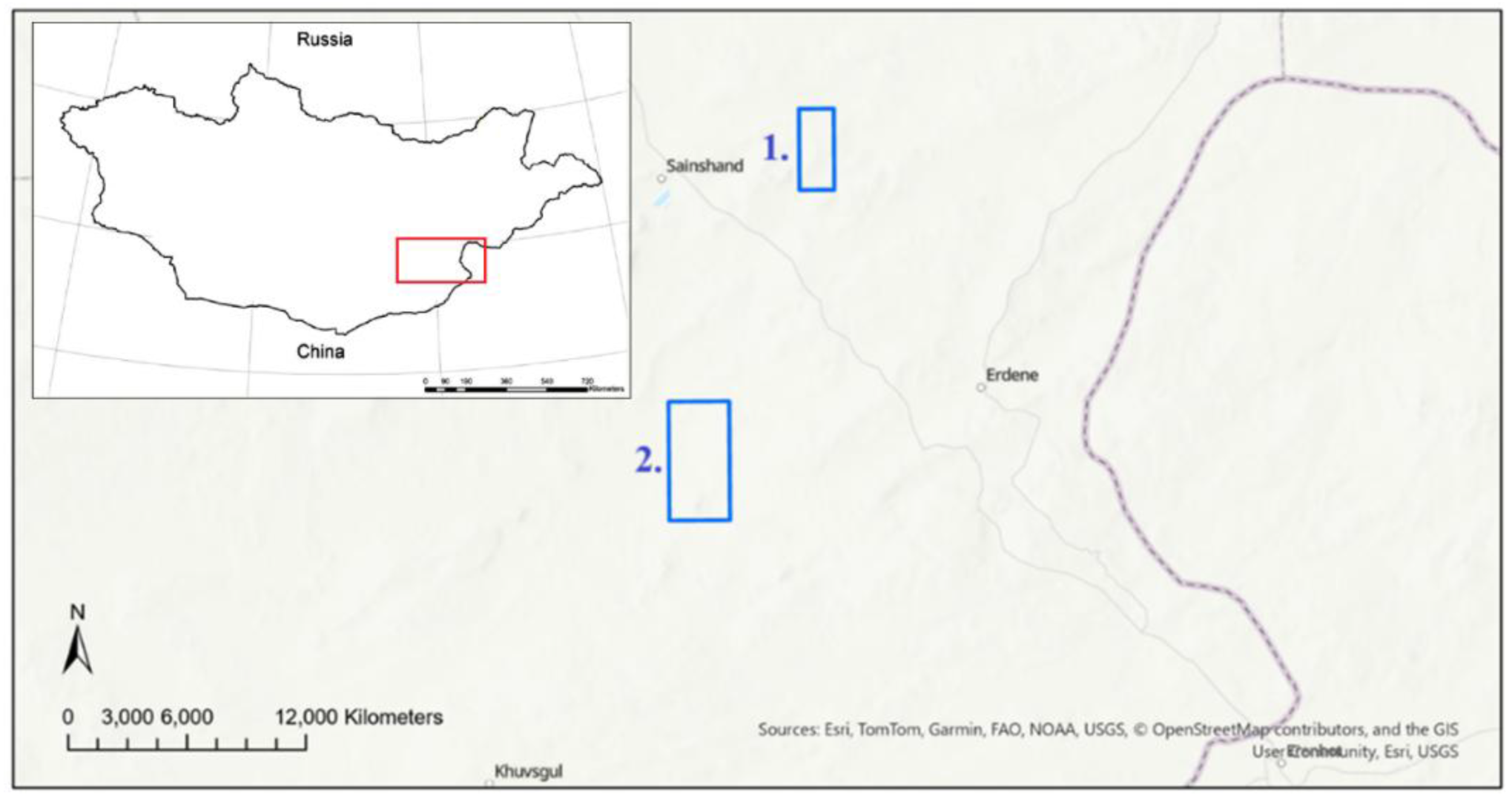
Figure 2.
Schematic representation of areas with increased radioactivity according to Soviet data (reports [11] and [14]) shown in orange and data from car-borne exploration from 2008 (anomalous values over 300 cps are in red).
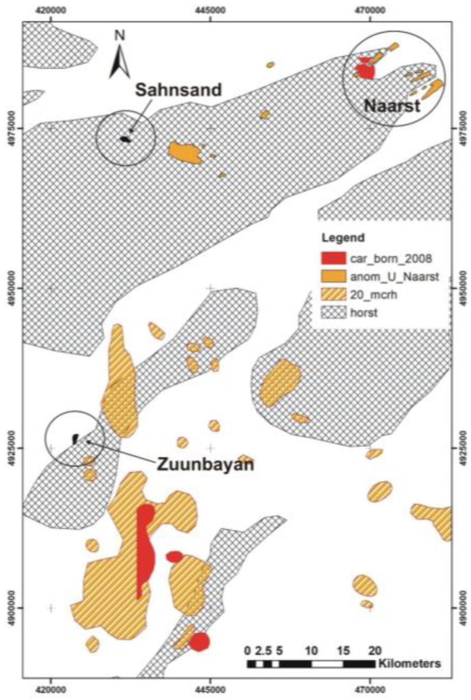
Figure 3.
a) Naarst area car-borne gamma survey (Summer 2008). Elevated counts here are influenced by anthropogenic sources—particularly historical drilling mud pits that concentrate radioactivity [15]; b) Zuunbayan area car-borne gamma survey (Summer 2008). Radioactivity in this region reflects natural levels [15].
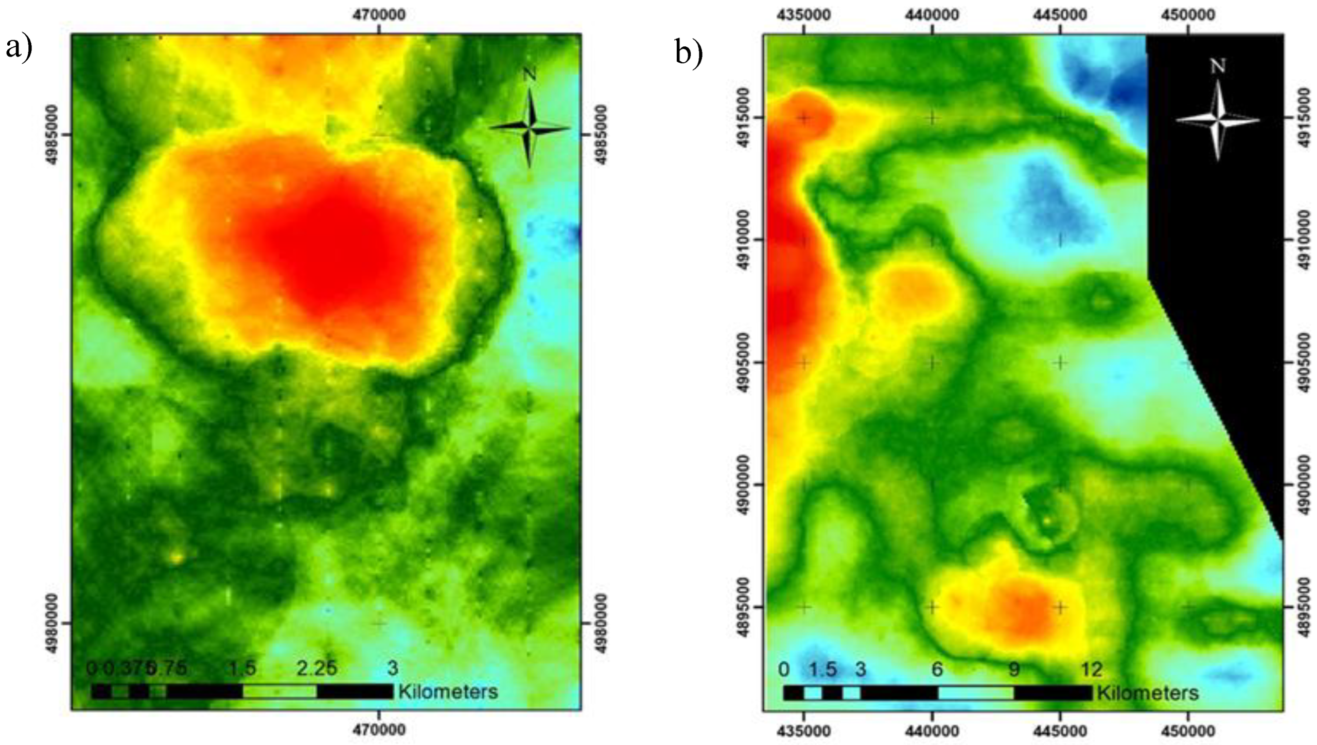
Figure 4.
Workflow diagram.
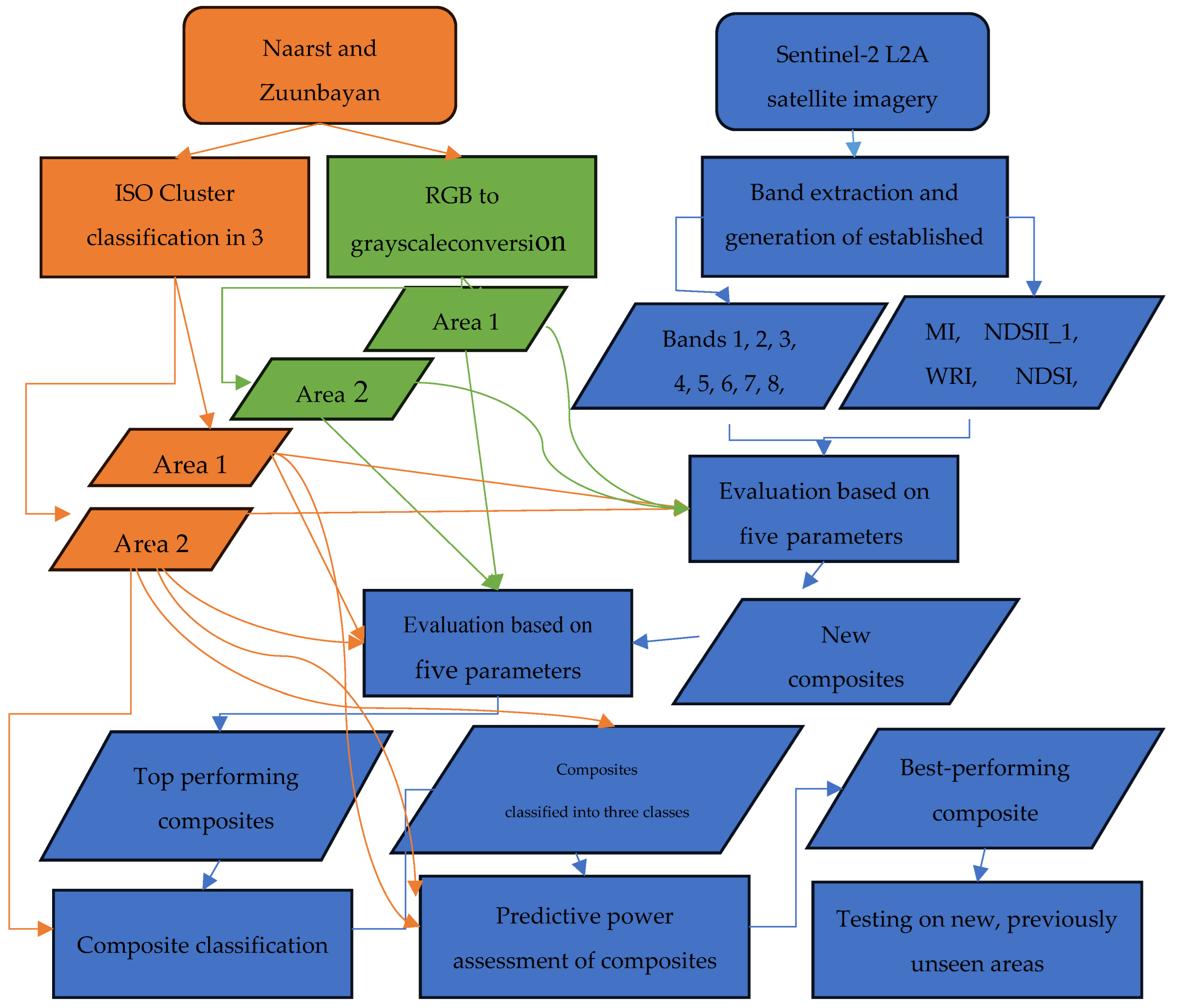
Figure 5.
RGB to grayscale transformation: Area 1 and Area 2 RGB heatmaps (A and C) [15], and their corresponding grayscale rasters (B and D).
Figure 5.
RGB to grayscale transformation: Area 1 and Area 2 RGB heatmaps (A and C) [15], and their corresponding grayscale rasters (B and D).
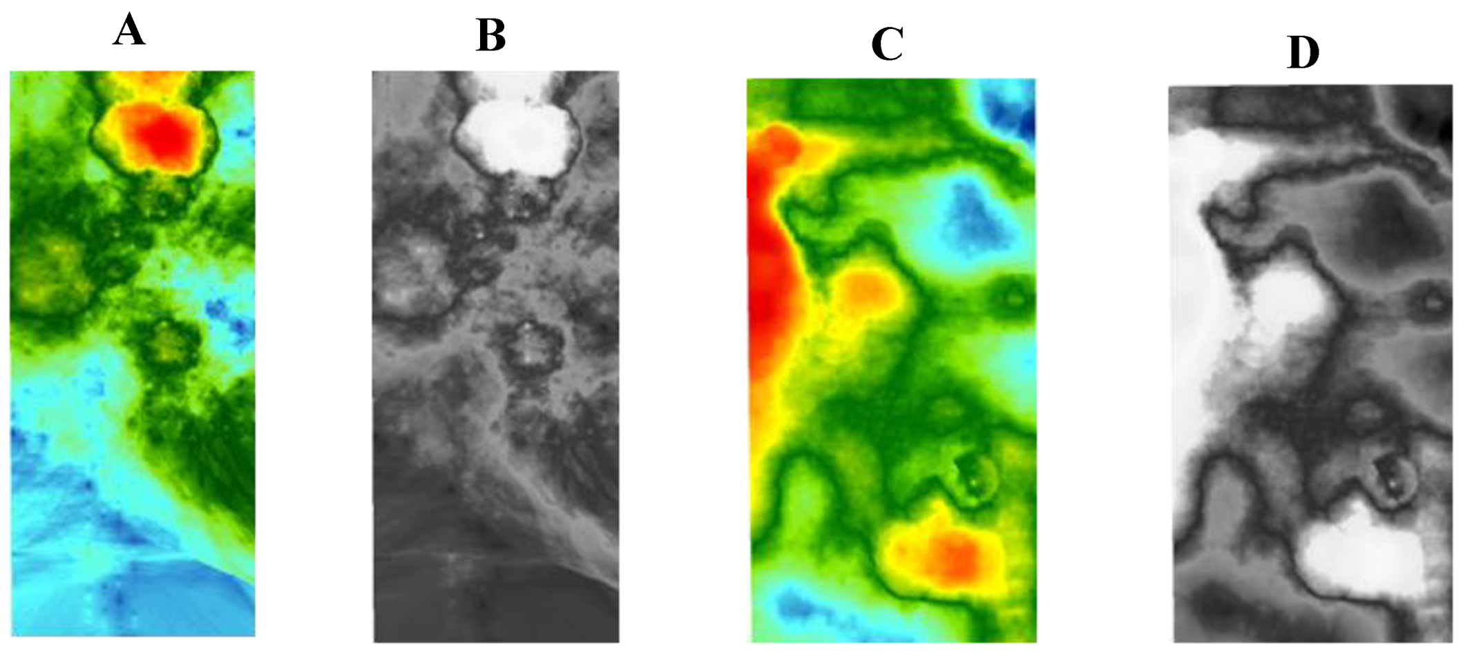
Figure 6.
Classification of the gamma-radiation heatmaps (Area 1 – A, Area 2 – D) using the ISO-Cluster classifier (Area 1 – B, Area 2 – E) and subsequent reclassification into three classes (Area 1 – C, Area 2 – F).
Figure 6.
Classification of the gamma-radiation heatmaps (Area 1 – A, Area 2 – D) using the ISO-Cluster classifier (Area 1 – B, Area 2 – E) and subsequent reclassification into three classes (Area 1 – C, Area 2 – F).
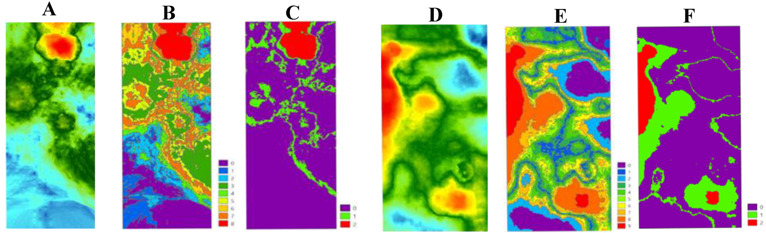
Figure 8.
The gamma radiation heatmap and the newly developed composite indices for Area 2.
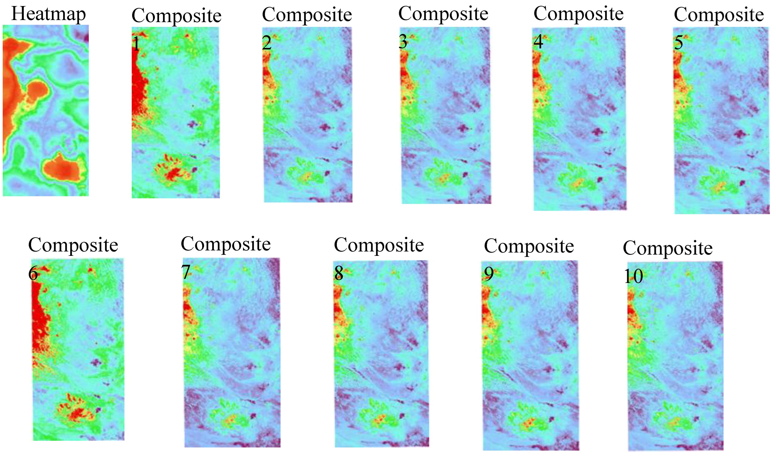
Figure 9.
Composite 7 overlaid with the classified gamma radiation raster of Area 2.
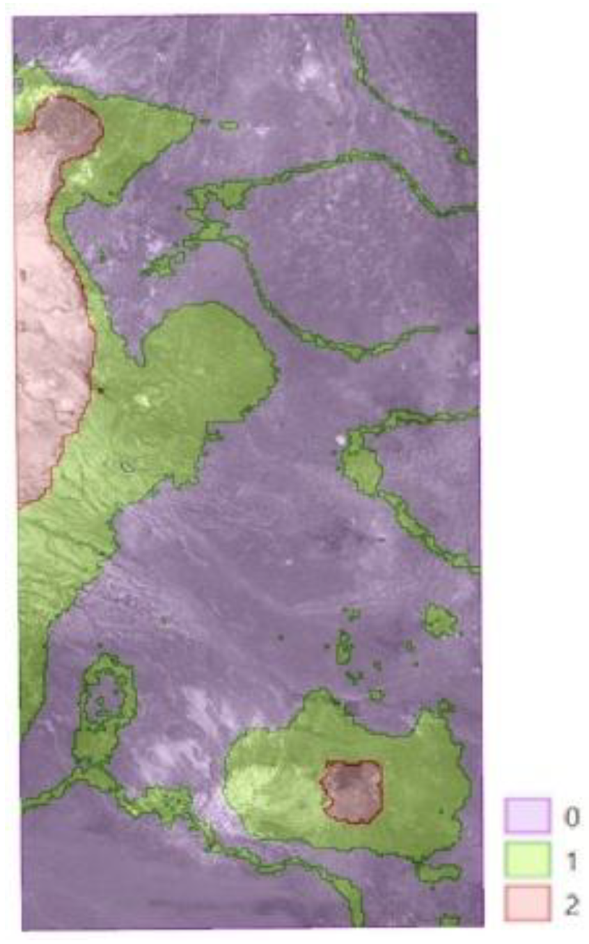
Figure 10.
Overlaid histogram with the computed boundaries between classes.
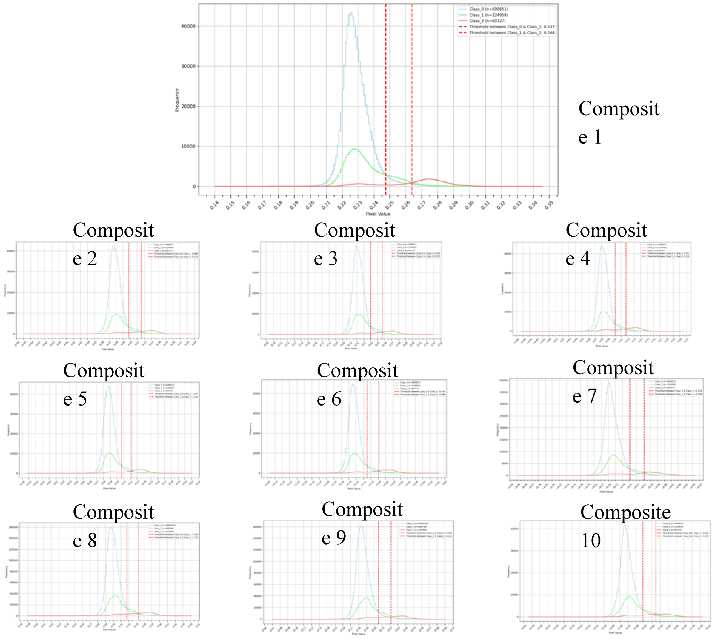
Figure 11.
Classified heatmap and composites in Area 2 (Class 2 – red, Class 1 – green, Class 0 – purple).
Figure 11.
Classified heatmap and composites in Area 2 (Class 2 – red, Class 1 – green, Class 0 – purple).
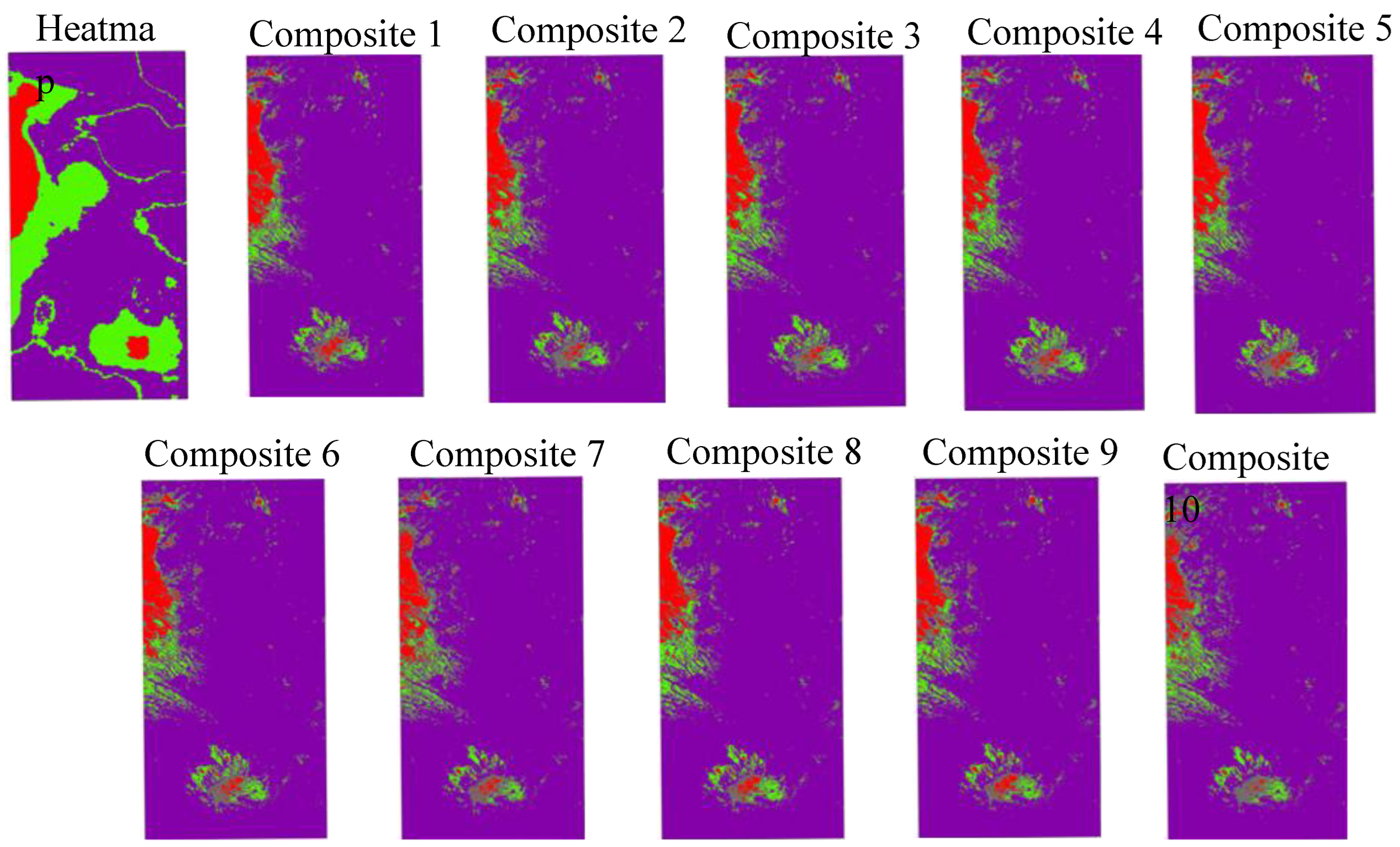
Figure 12.
Classified heatmap and composites in Area 1 (Class 2 – red; Class 1 – green; Class 0 – purple).
Figure 12.
Classified heatmap and composites in Area 1 (Class 2 – red; Class 1 – green; Class 0 – purple).
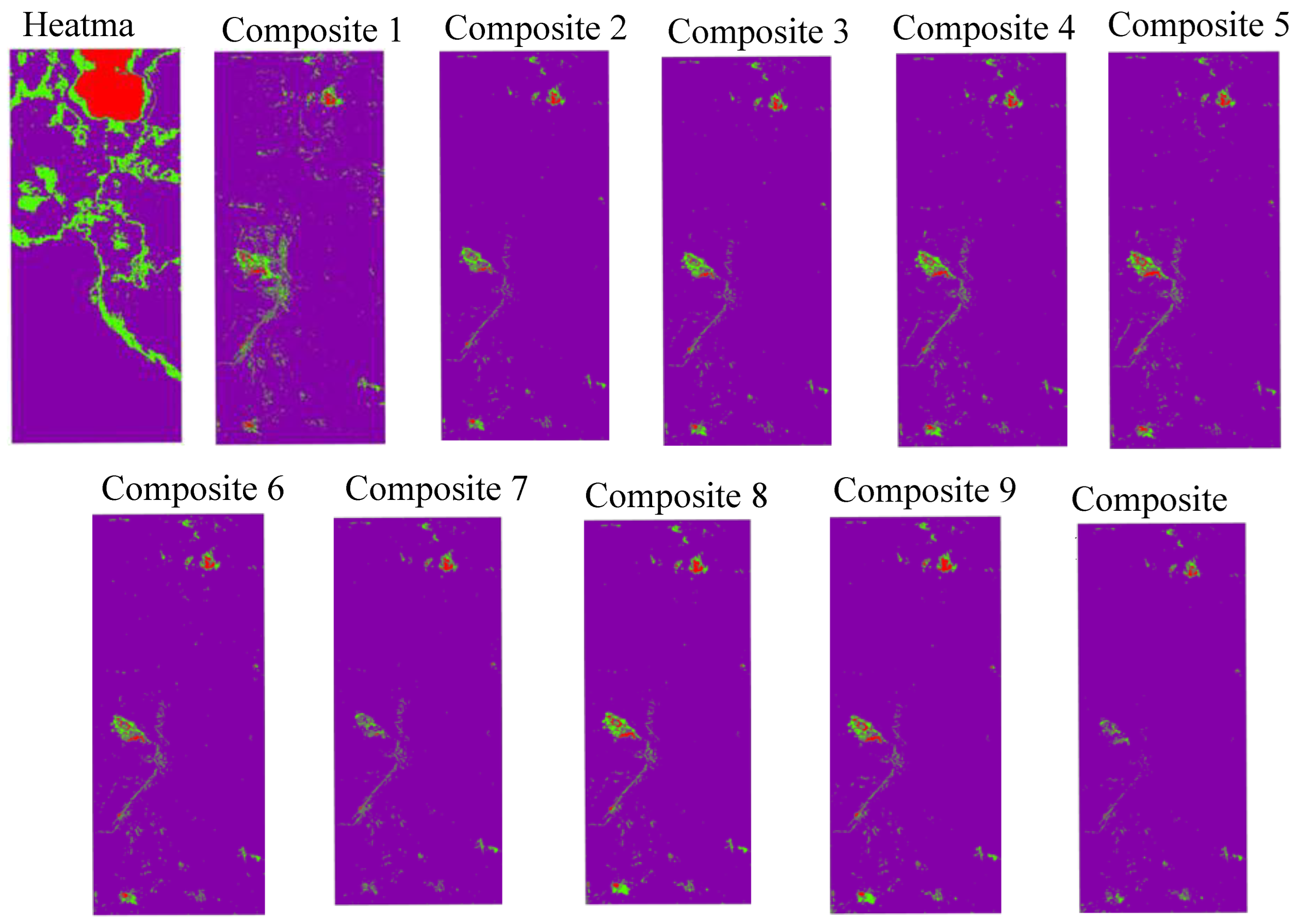
Figure 13.
Erdene study area: (A) original airborne gamma-spectrometry heatmap [25]; (B) classified heatmap with high-radiation areas shown in yellow and background in blue; (C) corresponding classified NDGRI raster highlighting pixel-level gamma-radiation anomalies.
Figure 13.
Erdene study area: (A) original airborne gamma-spectrometry heatmap [25]; (B) classified heatmap with high-radiation areas shown in yellow and background in blue; (C) corresponding classified NDGRI raster highlighting pixel-level gamma-radiation anomalies.
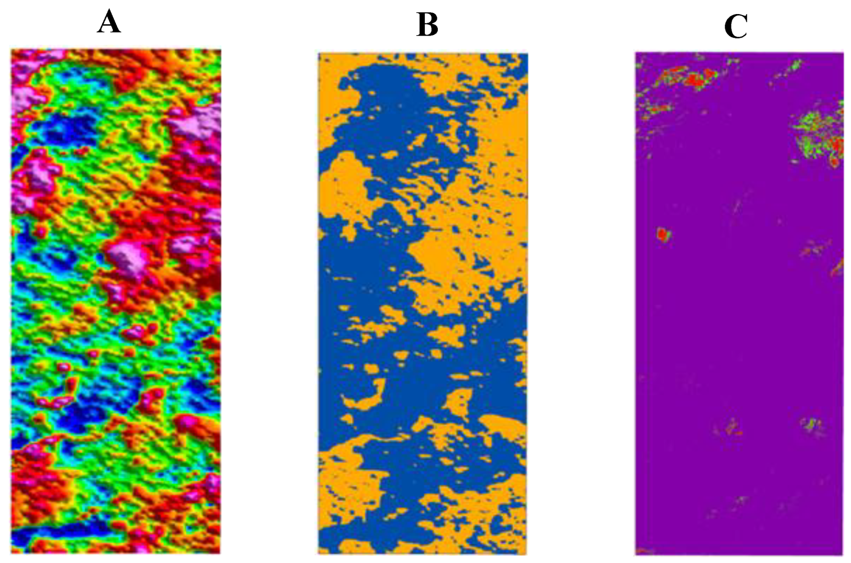
Figure 14.
Khuvsgul study area: (A) original airborne gamma-spectrometry heatmap [25]; (B) classified heatmap with high-radiation areas shown in yellow and background in blue; (C) corresponding classified NDGRI raster highlighting pixel-level gamma-radiation anomalies.
Figure 14.
Khuvsgul study area: (A) original airborne gamma-spectrometry heatmap [25]; (B) classified heatmap with high-radiation areas shown in yellow and background in blue; (C) corresponding classified NDGRI raster highlighting pixel-level gamma-radiation anomalies.
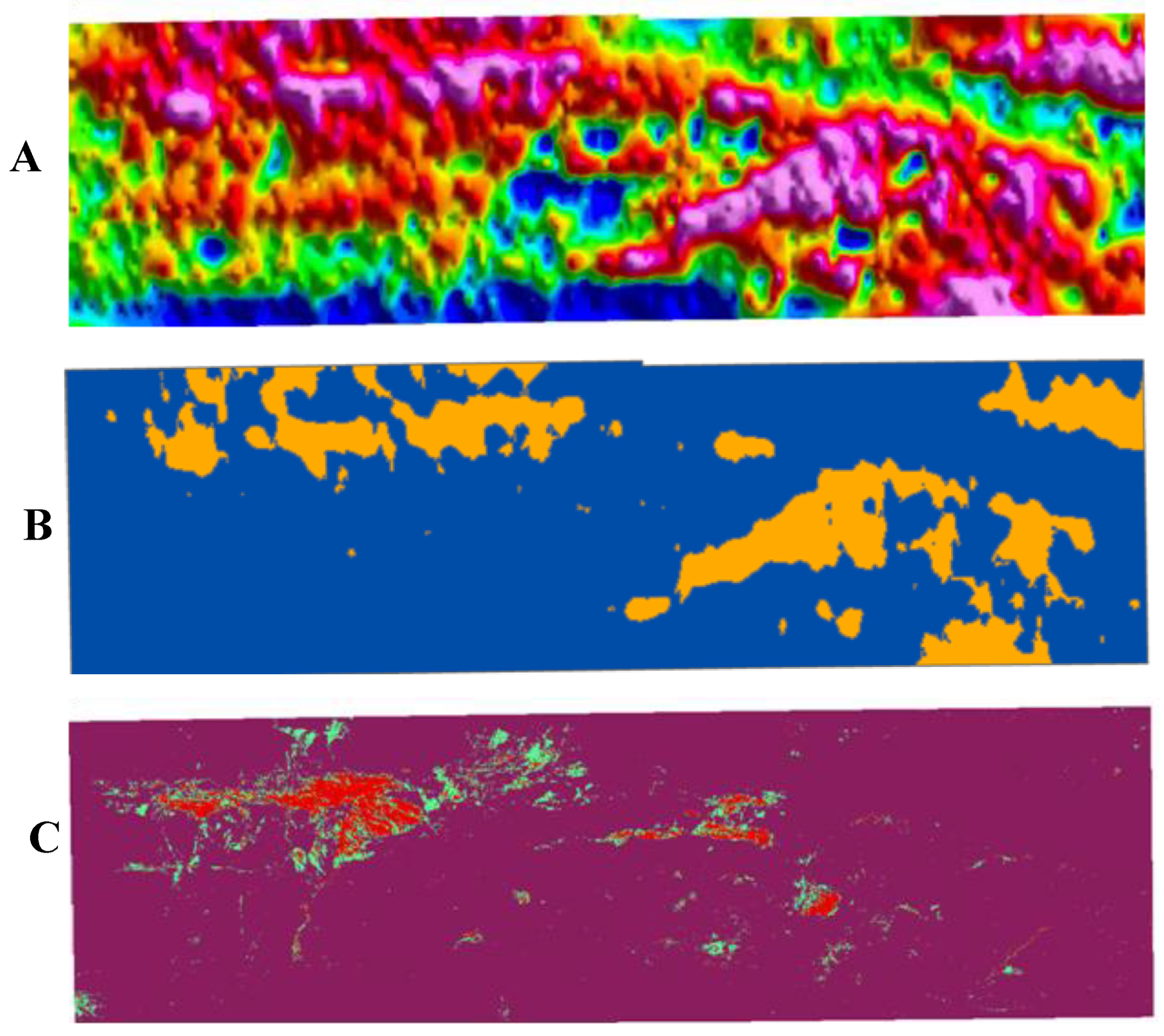
Figure 15.
Example Sentinel-2 scenes classified as usable or unusable for NDGRI screening.
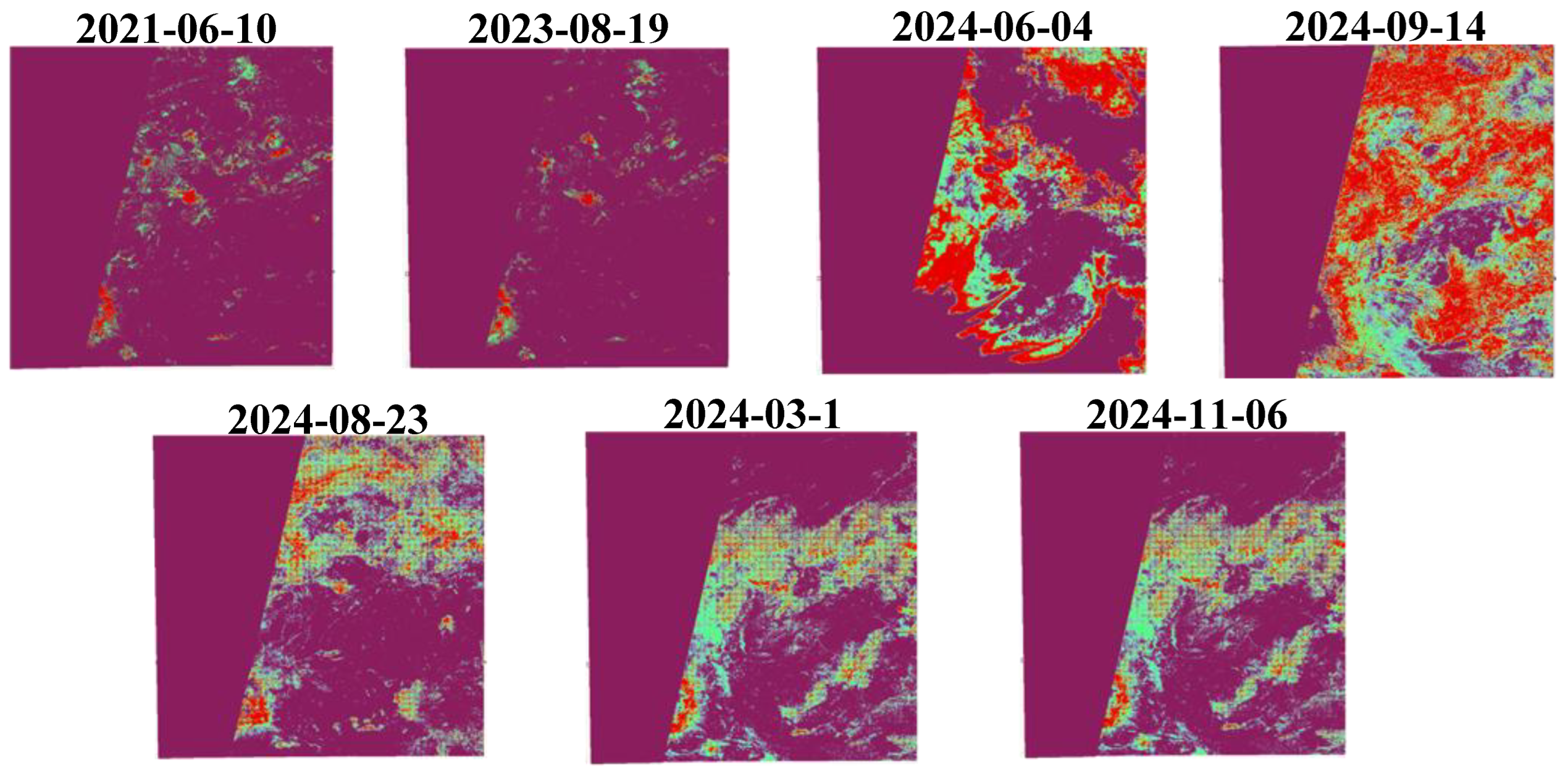

Table 1.
Composite and Spectral Band Scores for Sentinel 2.
| Area 2 | Area 1 | E | |||||||
| PC | SC | P1 | P2 | PC | SC | P1 | P2 | ||
| MI | 0.34 | 0.23 | 0.86 | 0.4 | 0.09 | 0.08 | 0.29 | 0.13 | 36.50% |
| NDSII_1 | 0.37 | 0.25 | 0.85 | 0.4 | -0.04 | -0.12 | 0.27 | 0.15 | 34.60% |
| WRI | 0.31 | 0.22 | 0.76 | 0.45 | -0.08 | -0.16 | 0.2 | 0.11 | 30.96% |
| NDSI | 0.29 | 0.2 | 0.74 | 0.41 | -0.09 | -0.17 | 0.19 | 0.1 | 28.86% |
| NDWI | 0.09 | 0.07 | 0.55 | 0.1 | -0.12 | -0.2 | 0.12 | 0.06 | 13.19% |
| B01 | 0.07 | 0.03 | 0.62 | 0.31 | 0.22 | 0.1 | 0.5 | 0.29 | 26.52% |
| B02 | 0.06 | 0.04 | 0.62 | 0.32 | 0.19 | 0.08 | 0.49 | 0.24 | 25.54% |
| B03 | 0.05 | 0.04 | 0.48 | 0.3 | 0.19 | 0.13 | 0.51 | 0.24 | 23.34% |
| B04 | 0.06 | 0.06 | 0.36 | 0.24 | 0.22 | 0.16 | 0.56 | 0.25 | 21.57% |
| B05 | 0.05 | 0.06 | 0.24 | 0.16 | 0.25 | 0.2 | 0.57 | 0.27 | 18.71% |
| B06 | 0.03 | 0.05 | 0.12 | 0.07 | 0.26 | 0.24 | 0.54 | 0.23 | 14.35% |
| B07 | 0.01 | 0.04 | 0.09 | 0.04 | 0.27 | 0.26 | 0.53 | 0.23 | 12.92% |
| B08 | -0.01 | 0.03 | 0.08 | 0.02 | 0.25 | 0.25 | 0.5 | 0.2 | 10.95% |
| B08A | -0.02 | 0.02 | 0.06 | 0.01 | 0.28 | 0.29 | 0.5 | 0.22 | 10.93% |
| B11 | -0.15 | -0.09 | 0.04 | 0 | 0.25 | 0.28 | 0.49 | 0.18 | 5.43% |
| B12 | -0.16 | -0.11 | 0.04 | 0 | 0.2 | 0.2 | 0.49 | 0.16 | 3.79% |
Table 3.
Class boundary values for each composite, showing the lower boundary first followed by the upper boundary.
Table 3.
Class boundary values for each composite, showing the lower boundary first followed by the upper boundary.
| Composite 1 | Composite 2 | Composite 3 | Composite 4 | Composite 5 | ||||||
| Class 2 | 0.26 | 0.35 | 0.12 | 0.19 | 0.26 | 0.33 | 0.12 | 0.21 | 0.12 | 0.21 |
| Class 1 | 0.25 | 0.26 | 0.10 | 0.12 | 0.24 | 0.26 | 0.10 | 0.12 | 0.11 | 0.12 |
| Class 0 | 0.14 | 0.25 | -0.04 | 0.10 | 0.09 | 0.24 | -0.04 | 0.10 | -0.03 | 0.11 |
| Composite 6 | Composite 7 | Composite 8 | Composite 9 | Composite 10 | ||||||
| Class 2 | -0.09 | -0.01 | -0.11 | -0.04 | 0.33 | 0.40 | 0.22 | 0.29 | -0.44 | -0.38 |
| Class 1 | -0.11 | -0.09 | -0.13 | -0.11 | 0.32 | 0.33 | 0.21 | 0.22 | -0.45 | -0.44 |
| Class 0 | -0.24 | -0.11 | -0.29 | -0.13 | 0.19 | 0.32 | 0.07 | 0.21 | -0.59 | -0.45 |
Table 2.
Scores of the New Theoretical Composites.
| Area 2 | Area 1 | E | ||||||||
| Formula | PC | SC | P1 | P2 | PC | SC | P1 | P2 | ||
| 1 | (B4 + B8A - B12) / (B4 + B8A + B12) | 0.39 | 0.26 | 0.89 | 0.74 | 0.17 | 0.16 | 0.38 | 0.16 | 46.58% |
| 2 | (B5 + B4 + B8A - B11 - B12) / (B4 + B5 + B8A + B11 + B12) | 0.41 | 0.28 | 0.88 | 0.71 | 0.09 | 0.02 | 0.37 | 0.19 | 44.89% |
| 3 | (B6 + B5 + B4 + B8A - B11 - B12) / (B6 + B4 + B5 + B8A + B11 + B12) | 0.41 | 0.28 | 0.89 | 0.72 | 0.08 | 0.02 | 0.35 | 0.18 | 44.88% |
| 4 | (B6 + B4 + B8A - B11 - B12) / (B4 + B6 + B8A + B11 + B12) | 0.4 | 0.27 | 0.88 | 0.72 | 0.09 | 0.04 | 0.35 | 0.17 | 44.78% |
| 5 | (B7 + B4 + B8A - B11 - B12) / (B4 + B7 + B8A + B11 + B12) | 0.4 | 0.27 | 0.88 | 0.72 | 0.09 | 0.06 | 0.35 | 0.16 | 44.74% |
| 6 | (B4 + B8A - B11 - B12) / (B4 + B8A + B11 + B12) | 0.41 | 0.27 | 0.88 | 0.7 | 0.1 | 0.05 | 0.37 | 0.18 | 44.72% |
| 7 | (B04 - B12) / (B04 + B12) | 0.4 | 0.26 | 0.88 | 0.68 | 0.08 | 0 | 0.39 | 0.19 | 43.85% |
| 8 | (B3 + B6 + B5 + B4 + B8A - B11 - B12) / (B3 + B6 + B4 + B5 + B8A + B11 + B12) | 0.41 | 0.29 | 0.85 | 0.66 | 0.05 | -0.02 | 0.33 | 0.17 | 42.72% |
| 9 | (B3 + B5 + B4 + B8A - B11 - B12) / (B3 + B4 + B5 + B8A + B11 + B12) | 0.41 | 0.29 | 0.84 | 0.64 | 0.05 | -0.03 | 0.33 | 0.17 | 42.01% |
| 10 | (B4 - B11 - B12) / (B4 + B11 + B12) | 0.4 | 0.26 | 0.87 | 0.63 | 0.01 | -0.08 | 0.34 | 0.18 | 41.18% |
| 11 | (B4 + B8A - B11) / (B4 + B8A + B11) | 0.4 | 0.28 | 0.86 | 0.65 | 0.01 | -0.07 | 0.29 | 0.16 | 41.08% |
| 12 | (B3 + B4 + B8A - B11 - B12) / (B4 + B3 + B8A + B11 + B12) | 0.4 | 0.28 | 0.82 | 0.61 | 0.04 | -0.03 | 0.33 | 0.16 | 40.80% |
| 13 | (B4 + B8 - B11) / (B4 + B8 + B11) | 0.38 | 0.26 | 0.86 | 0.62 | -0.02 | -0.09 | 0.26 | 0.14 | 39.15% |
| 14 | (B2 + B4 + B8A - B11 - B12) / (B4 + B2 + B8A + B11 + B12) | 0.38 | 0.27 | 0.8 | 0.57 | 0.02 | -0.06 | 0.3 | 0.15 | 38.71% |
| 15 | (B1 + B4 + B8A - B11 - B12) / (B4 + B1 + B8A + B11 + B12) | 0.39 | 0.28 | 0.8 | 0.56 | 0.03 | -0.04 | 0.29 | 0.15 | 38.60% |
| 16 | (B1 + B4 - B11 - B12) / (B4 + B1 + B11 + B12) | 0.35 | 0.25 | 0.76 | 0.47 | -0.05 | -0.14 | 0.24 | 0.13 | 33.15% |
Table 4.
Results of the Predictive Power Evaluation of the Composites.
| Area 1 | Area 2 | G | ||||||||
| P | R | F1 | OA | P | R | F1 | OA | |||
| Composite 1 | Class 2 | 0.72 | 0.63 | 0.67 | 0.75 | 0.26 | 0.03 | 0.06 | 0.77 | 5.84 |
| Class 1 | 0.52 | 0.15 | 0.23 | 0.07 | 0.02 | 0.03 | ||||
| Class 0 | 0.77 | 0.96 | 0.86 | 0.81 | 0.95 | 0.87 | ||||
| Composite 2 | Class 2 | 0.70 | 0.58 | 0.63 | 0.75 | 0.40 | 0.02 | 0.05 | 0.80 | 5.92 |
| Class 1 | 0.50 | 0.15 | 0.24 | 0.01 | 0.00 | 0.00 | ||||
| Class 0 | 0.77 | 0.96 | 0.86 | 0.81 | 0.98 | 0.89 | ||||
| Composite 3 | Class 2 | 0.72 | 0.58 | 0.64 | 0.75 | 0.35 | 0.02 | 0.04 | 0.79 | 5.88 |
| Class 1 | 0.50 | 0.16 | 0.24 | 0.01 | 0.00 | 0.00 | ||||
| Class 0 | 0.77 | 0.96 | 0.86 | 0.81 | 0.98 | 0.89 | ||||
| Composite 4 | Class 2 | 0.71 | 0.59 | 0.64 | 0.75 | 0.28 | 0.02 | 0.05 | 0.79 | 5.74 |
| Class 1 | 0.50 | 0.16 | 0.24 | 0.02 | 0.00 | 0.01 | ||||
| Class 0 | 0.77 | 0.96 | 0.86 | 0.81 | 0.98 | 0.88 | ||||
| Composite 5 | Class 2 | 0.70 | 0.61 | 0.65 | 0.75 | 0.25 | 0.03 | 0.05 | 0.79 | 5.70 |
| Class 1 | 0.51 | 0.14 | 0.22 | 0.03 | 0.00 | 0.01 | ||||
| Class 0 | 0.77 | 0.96 | 0.86 | 0.81 | 0.98 | 0.88 | ||||
| Composite 6 | Class 2 | 0.69 | 0.58 | 0.63 | 0.75 | 0.32 | 0.03 | 0.05 | 0.79 | 5.77 |
| Class 1 | 0.50 | 0.15 | 0.23 | 0.02 | 0.00 | 0.01 | ||||
| Class 0 | 0.77 | 0.96 | 0.86 | 0.81 | 0.98 | 0.89 | ||||
| Composite 7 | Class 2 | 0.69 | 0.54 | 0.60 | 0.75 | 0.57 | 0.03 | 0.06 | 0.80 | 6.09 |
| Class 1 | 0.50 | 0.14 | 0.22 | 0.02 | 0.00 | 0.00 | ||||
| Class 0 | 0.77 | 0.96 | 0.86 | 0.81 | 0.99 | 0.89 | ||||
| Composite 8 | Class 2 | 0.67 | 0.53 | 0.59 | 0.75 | 0.34 | 0.03 | 0.06 | 0.79 | 5.61 |
| Class 1 | 0.48 | 0.15 | 0.22 | 0.01 | 0.00 | 0.00 | ||||
| Class 0 | 0.77 | 0.96 | 0.86 | 0.81 | 0.98 | 0.88 | ||||
| Composite 9 | Class 2 | 0.65 | 0.51 | 0.57 | 0.75 | 0.37 | 0.03 | 0.06 | 0.79 | 5.58 |
| Class 1 | 0.49 | 0.14 | 0.22 | 0.01 | 0.00 | 0.00 | ||||
| Class 0 | 0.77 | 0.96 | 0.85 | 0.81 | 0.98 | 0.88 | ||||
| Composite 10 | Class 2 | 0.69 | 0.46 | 0.55 | 0.74 | 0.64 | 0.02 | 0.04 | 0.80 | 5.99 |
| Class 1 | 0.47 | 0.16 | 0.24 | 0.01 | 0.00 | 0.00 | ||||
| Class 0 | 0.77 | 0.96 | 0.85 | 0.81 | 0.99 | 0.89 | ||||
Table 5.
Metadata for example Sentinel-2 scenes deemed usable or unusable for NDGRI screening.
| Acquisition day | 2021-06-10 | 2023-08-19 | 2024-06-04 | 2024-09-14 | 2024-08-23 | 2024-03-11 | 2024-11-06 |
| Cloud cover (%) | 0.00% | 0.00% | 65.69% | 0.06% | 2.34% | 0.24% | 0.00% |
| Vegetation cover (%) | 0.00% | 0.03% | 0.00% | 0.71% | 3.00% | 0.00% | 0.00% |
| Snow & Ice (%) | 0.00% | 0.00% | 0.00% | 0.00% | 0.00% | 26.13% | 0.00% |
| Mean water vapor (g/cm²) | 0.58 | 0.97 | 1.42 | 0.63 | 2.51 | 0.26 | 0.45 |
| Rain on acquisition day (mm) | - | - | 26 mm | - | - | - | - |
| Rain in prior days (mm) | 01.06. - 1 mm | 10.08. - 0.4 mm | - | 12.09. - 21 mm | 22.08. - 11 mm | - | 20.10. - 3 mm |
| Temp °C (mean/min/max) | 26.0 / 14.5 / 32.2 | 24.4 / 11.4 / 30.5 | 21.0 / 16.0 / 30.8 | 9.7 / 2.1 / 15.0 | 22.3 / 16.8 / 27.8 | -5.5 / -13.9 / 0.4 | 0.2 / -5.6 / 7.6 |
| Verdict | Usable | Usable | Unusable (heavy rain & clouds) | Unusable (residual moisture) | Unusable (residual moisture) | Unusable (snow & ice) | Unusable (freeze-thaw moisture) |
Disclaimer/Publisher’s Note: The statements, opinions and data contained in all publications are solely those of the individual author(s) and contributor(s) and not of MDPI and/or the editor(s). MDPI and/or the editor(s) disclaim responsibility for any injury to people or property resulting from any ideas, methods, instructions or products referred to in the content. |
© 2025 by the authors. Licensee MDPI, Basel, Switzerland. This article is an open access article distributed under the terms and conditions of the Creative Commons Attribution (CC BY) license (http://creativecommons.org/licenses/by/4.0/).
Copyright: This open access article is published under a Creative Commons CC BY 4.0 license, which permit the free download, distribution, and reuse, provided that the author and preprint are cited in any reuse.


