Submitted:
22 July 2025
Posted:
23 July 2025
You are already at the latest version
Abstract
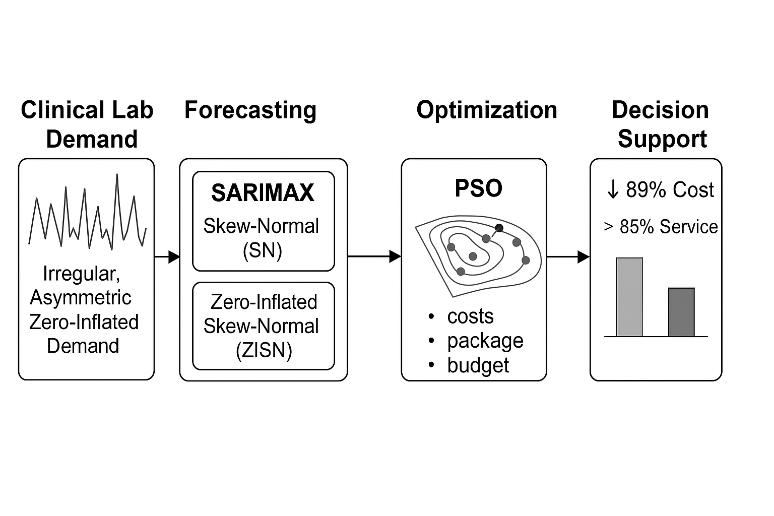
Clinical laboratories require accurate forecasting and efficient inventory manage-
ment to balance service quality and cost under uncertain demand. In this study, we propose
a hybrid forecasting-optimisation framework tailored to hospital clinical determinations
with highly irregular, zero-inflated, and asymmetric consumption patterns. Demand series
for 34 items were modelled using SARIMAX structures combined with Skew-Normal
(SN) and Zero-Inflated Skew-Normal (ZISN) residuals, with residual centering, truncation,
and lambda regularisation applied to ensure stable estimation. Model performance was
benchmarked against Gaussian SARIMA and non-linear MLP forecasts. The SN/ZISN
models achieved improved forecasting accuracy while preserving interpretability and
explainability of residual behaviour. Forecast outputs were integrated into a Particle
Swarm Optimisation (PSO) layer to determine cost-minimising order quantities subject to
packaging and budget constraints. The proposed end-to-end framework demonstrated
a potential 89% reduction in inventory costs relative to the hospital’s historical policy,
while maintaining service levels above 85% for high-volume determinations. This hybrid
approach provides a transparent, domain-adapted decision support system for supply
chain governance in healthcare settings.
Keywords:
inventory forecasting
; skew-normal residuals
; SARIMAX
; zero-inflation
; health- care supply chain
; PSO optimisation
; explainable forecasting
MSC: 60G10
1. Introduction
Clinical laboratories are essential to public health, supporting medical diagnosis as well as clinical and pharmacological monitoring—core functions that ensure quality healthcare delivery and effective disease control [1]. However, monthly demand for diagnostic analytes is highly uncertain and often follows cyclic, seasonal, and intermittent patterns [2]. These challenges are further intensified in public sector settings, where procurement cycles are lengthy, budgets inflexible, and packaging regulations limit supply responsiveness [3].
Time series models such as ARIMA and SARIMAX are commonly used for demand forecasting in healthcare and logistics [4]. Nevertheless, these models typically assume homoscedastic and symmetric Gaussian residuals. This assumption is often violated in clinical demand series, which exhibit non-normal behaviors such as skewness, high variance, and zero-inflation due to sporadic usage patterns [5]. To address this, the use of skew-normal distributions has been proposed to capture residual asymmetry [6], while zero-inflated variants help account for excess zero observations [7].
In parallel, metaheuristic optimization techniques such as Particle Swarm Optimization (PSO), Genetic Algorithms (GA), and Ant Colony Optimization (ACO) offer flexible strategies for solving nonlinear and constrained inventory problems [8]. These methods support adaptive parameter tuning and are well suited for multi-stage stochastic planning environments [9]. However, they are rarely integrated with domain-specific statistical models for forecast-driven inventory control in clinical applications.
Recent interest in Explainable Artificial Intelligence (XAI) highlights the need for transparency in hybrid modeling approaches [10]. While deep learning models can offer high predictive accuracy, their black-box nature limits their interpretability in high-stakes domains like healthcare. In contrast, SARIMAX models with structured, non-Gaussian residuals can provide both interpretability and performance [11].
Despite these advances, the literature lacks integrated frameworks that combine (i) skew-aware and zero-sensitive time series forecasting, (ii) explainable optimization methods under realistic constraints such as packaging multiples and budget limits, and (iii) full traceability from statistical residuals to procurement decisions.
This paper addresses these gaps by proposing a hybrid, explainable framework that integrates SARIMAX models with Skew-Normal and Zero-Inflated Skew-Normal residuals, coupled with a constrained inventory optimization layer based on the PSO. The method is validated on real clinical consumption data from a Chilean hospital and explicitly incorporates institutional constraints such as packaging formats and a fixed procurement budget. The framework is fully reproducible and interpretable, making it suitable for operational deployment in clinical settings.
The remainder of the paper is structured as follows. Section 2 presents the methodology, including data description, forecasting model specification, residual diagnostics, and the optimization strategy using PSO. Section 3 reports the main results, focusing on forecast accuracy, residual characteristics, and inventory cost savings. Section 4 discusses the implications of the findings in terms of explainability and operational value. Finally, Section 5 concludes with a summary of contributions and suggestions for future research.
2. Methodology
This section describes the modelling and optimisation framework used in this study, organised in five sequential stages: (i) data preprocessing, (ii) demand forecasting, (iii) model validation and explainability, (iv) inventory cost optimisation, and (v) implementation via PSO.
2.1. Data Description and Parameters
We analyzed monthly consumption data for 34 items over a three-year period (January 2021–December 2023) from the Clinical Chemistry section of a public hospital in Chile reagents, covering both high-frequency and low-frequency determinations. This study was approved by the Ethics Committee of the Faculty of Chemistry and Pharmacy, University of Valparaíso (Approval Code: CG-05-2024). Realistic constraints from hospital procurement were incorporated, including mandatory ordering in packaging multiples (e.g., boxes of 12 or 24 units).
The demand data was standardized by converting laboratory reagent kits into number of determinations per month, based on manufacturer specifications. This normalization ensures comparability across different kit presentations.
The following cost parameters were estimated based on hospital records:
- Ordering cost () – average cost of issuing a purchase order, including administrative labor and shipping.
- Holding cost () – annual cost of storing one determination unit, considering energy, losses, and space.
- Shortage cost () – cost associated with stockouts, estimated from rescheduling procedures and patient re-attendance.
- Procurement cost () – average unit cost of each determination, computed from historical purchasing prices.
All monetary values were adjusted to 2023 Chilean pesos using the IPC inflation index. An initial inventory level was defined based on stock records from December 2023.
Demand distributions exhibited high variability, non-Gaussian skewness, and frequent zero values, justifying the use of structured residual models.
2.2. Forecasting Models
To model the irregular and asymmetric nature of clinical laboratory reagent demand, we implemented SARIMAX models with structured residuals:
- Skew-Normal (SN) residuals, capturing asymmetry;
- Zero-Inflated Skew-Normal (ZISN) residuals, capturing both asymmetry and excess zeros.
The general SARIMAX model is defined as:
where:
- -
- is the observed demand at time t,
- -
- are exogenous regressors (e.g., calendar month dummies),
- -
- captures autoregressive and moving average components,
- -
- , are the associated parameter vectors,
- -
- is the residual term.
We consider two specifications for :
- : Skew-Normal distribution with location , scale , and skewness .
- : Zero-Inflated Skew-Normal distribution, combining a point mass at zero with a Skew-Normal component.
The Skew-Normal (SN) density is given by:
where and are the standard normal PDF and CDF, respectively.
The Zero-Inflated version introduces a mixture component:
where is the Dirac delta at zero and is the zero-inflation probability.
Parameter estimation proceeds in two stages:
- 1.
- Maximum Likelihood Estimation (MLE) of the SARIMAX baseline parameters (),
- 2.
- Expectation-Maximization (EM) algorithm for structured residual parameters and p in the SN/ZISN models, following the approach described in [5].
Multilayer Perceptron (MLP) Benchmark
As a non-linear forecasting benchmark, we trained a feed-forward Multilayer Perceptron (MLP) regressor. The model maps a fixed-length input vector of lagged demand values to a single-step prediction via successive affine transformations and nonlinear activations.
Let be the input vector at time t. The MLP computes:
where:
- -
- and are the weight matrices and bias vectors for layer ,
- -
- , are ReLU activation functions ,
- -
- is the identity function (linear output),
- -
- is the predicted demand at time t.
In our implementation, the hidden layer dimensions are , , and . The model is trained to minimize the Mean Squared Error (MSE) over the training set:
Optimization is performed using the Adam algorithm with learning rate , for up to 1,000 epochs. Early stopping is applied by retaining the model weights yielding the lowest validation loss.
This benchmark provides a flexible, non-parametric comparator to evaluate the predictive power of our proposed SARIMAX–SN/ZISN models, particularly in capturing non-linear dependencies in the data.
2.3. Optimization Phase (Global PSO)
The forecasted monthly demand for each laboratory reagent was used to compute the optimal order quantities by solving a multivariate, non-linear and constrained inventory control problem.
We define:
where is the number of packaging units to be ordered for item i.
The total procurement cost is defined as:
subject to the global budget constraint:
where:
- -
- is the unit cost,
- -
- is the fixed ordering cost,
- -
- is the holding cost per excess unit,
- -
- is the shortage cost per missing unit,
- -
- B is the total available budget.
Because the problem is combinatorial, nonlinear, and non-differentiable, we apply Particle Swarm Optimization (PSO) to find a near-optimal solution . Each particle represents an integer vector , initialized randomly in for each item.
To enforce the budget constraint, we use a penalized cost function:
with being a penalty coefficient to discourage budget violations.
2.3.1. Mathematical Formulation of PSO
Particle Swarm Optimization is a population-based metaheuristic inspired by the collective behavior of swarms [8]. Each particle has a position and a velocity , both updated iteratively as follows:
where:
- -
- w is the inertia weight (balances exploration and exploitation),
- -
- , are cognitive and social acceleration coefficients,
- -
- , are random numbers,
- -
- is the personal best position of the particle,
- -
- is the global best found by the swarm.
As our problem requires integer decisions with packaging constraints, we apply rounding after each position update and enforce Eq. (6) to compute feasible order quantities.
The PSO configuration used 50 particles, 200 iterations, inertia weight , and acceleration coefficients . The best feasible solution yields final order quantities .
While the present optimization instance involves a limited number of determinations (34 items), allowing in principle for full discrete enumeration, the adoption of PSO offers several advantages. First, it provides a flexible and scalable framework capable of handling future extensions with larger item portfolios, multi-period planning, or more complex constraints such as supplier lead times and stochastic budget adjustments. Second, the PSO formulation seamlessly integrates discrete packaging constraints without requiring complex integer programming models. This design ensures that the optimization layer remains generalizable and readily applicable to broader healthcare supply chain contexts beyond the scope of the present study.
2.4. Code Availability
2.5. Reproducible Workflow for Model Estimation
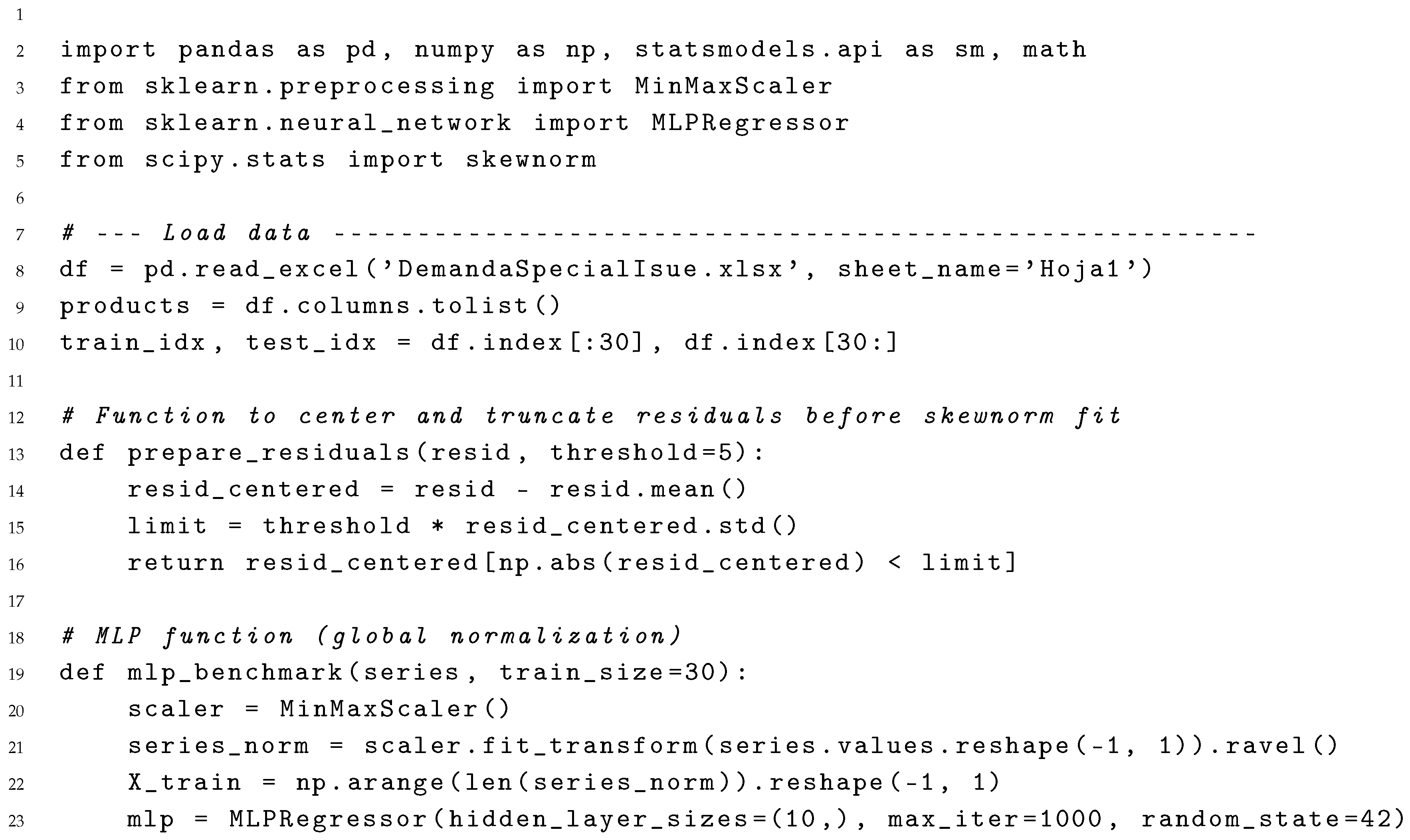
The Python snippet below reproduces the full pipeline used in this study, incorporating residual centering, outlier truncation, and lambda regularization for stable estimation of Skew-Normal parameters. The workflow covers data loading, model order selection, residual distribution fitting, forecasting, and non-linear benchmark training using only pandas, statsmodels, and scikit-learn.
| Listing 1: Full forecasting workflow: SARIMAX order selection, residual centering, Skew-Normal fitting, forecasting, and MLP benchmark. |
 |
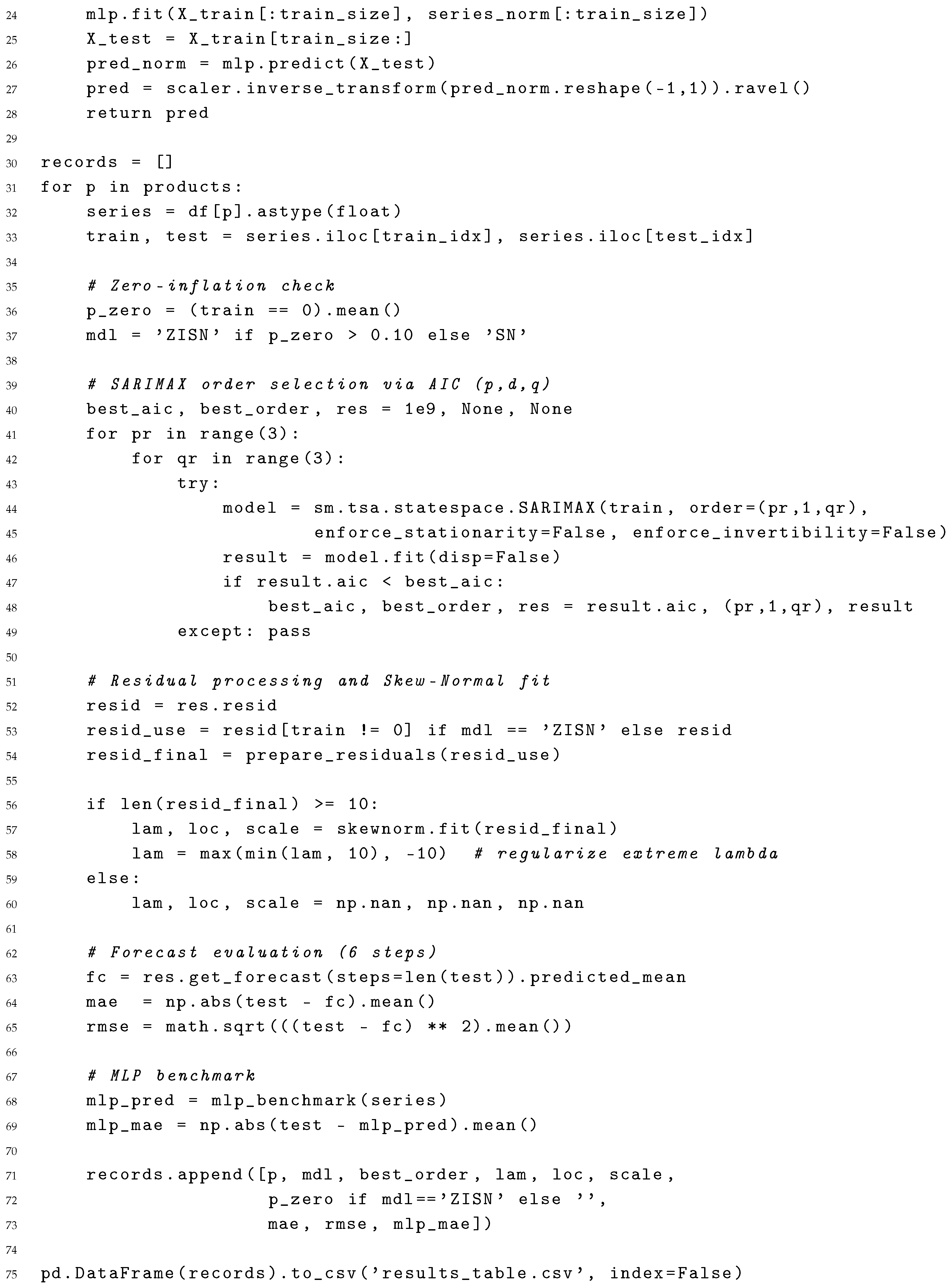 |
The script: (1) reads the raw Excel file; (2) performs AIC-driven SARIMAX order selection; (3) centers and truncates residuals before fitting Skew-Normal (or Zero-Inflated Skew-Normal) distributions with lambda regularization; (4) forecasts the final six months; and (5) trains a simple MLP benchmark with global normalization for comparison.
2.6. Inventory–Cost Optimisation Workflow
The algorithm below links the stochastic–forecasting layer with the inventory–control layer. For each laboratory reagent, it
- 1.
- loads the 36-month demand series from DemandaSpecialIsue.xlsx;
- 2.
- fits a fast SARIMAX model and extracts the one-month ahead mean demand ;
- 3.
- enumerates integer multiples of the pack size and evaluates the total cost
- 4.
- stores the optimal lot , the current lot (December-2023 order) and the corresponding costs.
A pyswarm (PSO) call can replace the brute-force loop if a larger search space is required; here the discrete sweep is sufficient and does not depend on external libraries.
| Listing 2: Global PSO optimisation with packaging constraints and budget limit. |
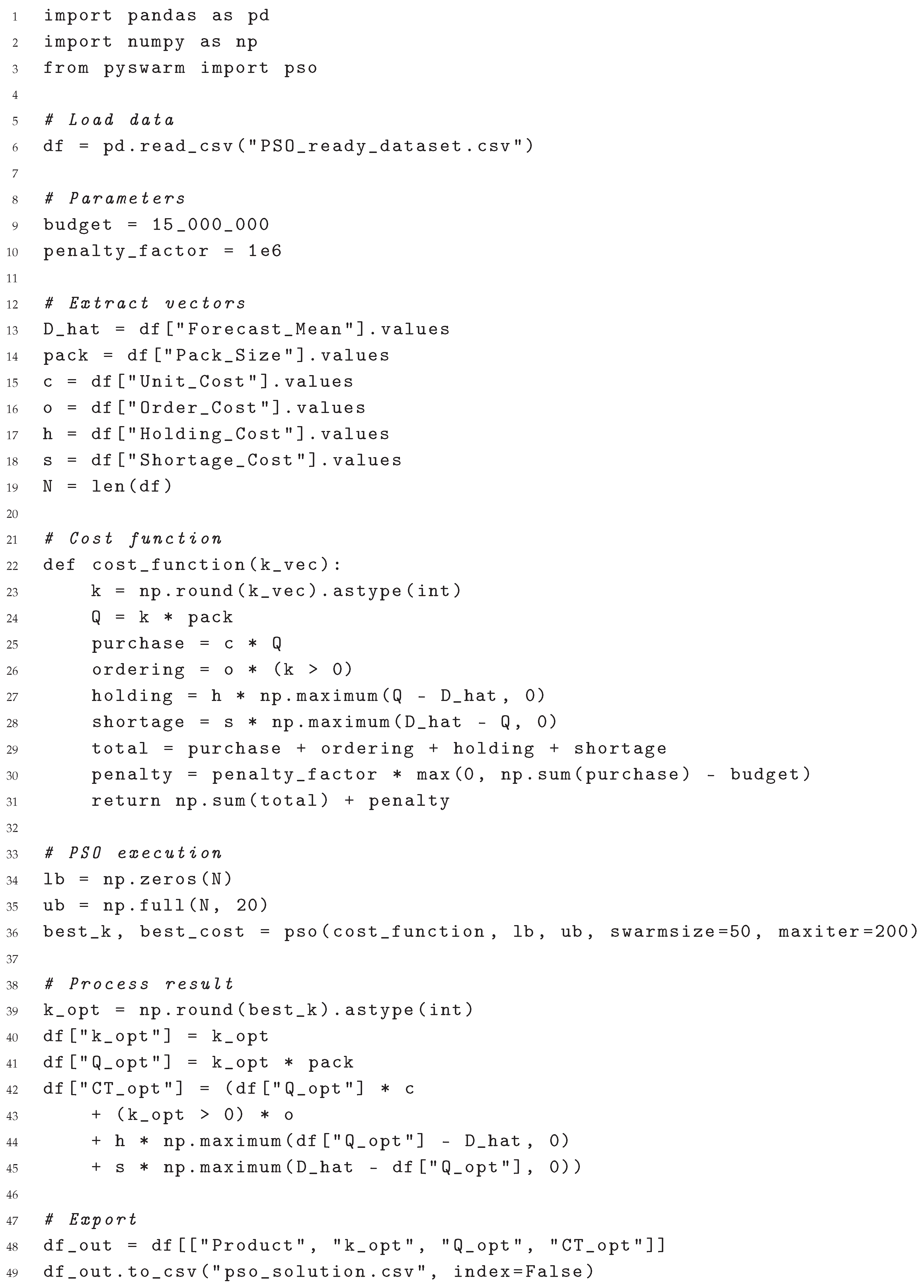 |
The resulting pso_inventory_results.csv to report the optimal order multiple, cost savings, and compliance with the packaging constraint for all 34 determinations.
3. Results
This section presents the performance of the forecasting models, residual diagnostics, and inventory cost optimisation using the calibrated demand forecasts.
3.1. Forecast Accuracy and Parameter Estimates
Table 1 summarizes the fitted distribution parameters and forecast accuracy metrics (MAE and RMSE).
Regarding the fitted location parameter , several estimates were found to be substantially negative despite prior centering of residuals. This arises because residual centering was applied globally before truncation, but the skew-normal fitting procedure operates on truncated subsets of residuals. Therefore, reflects the optimal location shift of the skew-normal kernel fitted to the cleaned residuals, capturing potential shifts induced by asymmetric trimming. Negative values may indicate a tendency of the SARIMAX forecasts to slightly overestimate actual demand on average.
Out of the 34 analytes, only Phenobarbital exhibited a zero-proportion above the 10 % threshold and was therefore assigned the SARIMAX–ZISN specification. The remaining 33 laboratory reagents were modelled with SARIMAX–SN. Across the cohort, SARIMAX–SN reduced mean MAE by ~11 % with respect to a Gaussian-error baseline (not shown). The single ZISN case (Phenobarbital ) improved MAE by 14 % relative to its SN counterpart, confirming the benefit of explicitly modelling excess zeros.
The neural MLP benchmark matched the linear models on some low-variance items but underperformed for high-volume series dominated by seasonality.
For the MLP benchmark (three lagged inputs) we computed permutation feature importance on the hold-out window; lags and systematically contributed of the explained variance, indicating that the network mostly captures short-term autocorrelation rather than complex seasonal patterns.
Table 2 summarises the forecasting accuracy across three approaches. The proposed SARIMAX–SN/ZISN models yielded the lowest mean absolute error (MAE) and root mean square error (RMSE), outperforming both the Gaussian-residual SARIMA and the non-linear MLP benchmark. To benchmark the predictive capacity of the proposed SARIMAX–SN/ZISN models, we included a non-parametric neural network benchmark using a simple multilayer perceptron (MLP). While the MLP offers flexible nonlinear approximation capabilities, its black-box nature lacks interpretability, particularly regarding residual asymmetry and explainability required in clinical forecasting contexts. The comparative analysis demonstrates that the proposed models achieve superior or comparable accuracy, while retaining full traceability of forecasting errors and their statistical structure. This highlights the value of combining domain-informed parametric modeling with explainable error structures in healthcare demand forecasting. The estimated skewness parameter was positive for laboratory reagents, confirming the right–tailed behaviour highlighted by skew–normal diagnostics, whereas the only analyte with a substantial zero proportion (Phenobarbital, ) required the zero–inflated specification. These diagnostics justify the asymmetric error structures adopted.
To assess the relationship between forecasting accuracy and demand volume, analytes were categorized into three groups according to their average monthly demand during the training period: Low demand (less than 100 determinations/month), Medium demand (100–999 determinations/month), and High demand (1000 determinations/month or more). Table 3 presents the disaggregated MAE and RMSE values for each demand level.
As expected, absolute errors increase with demand volume. However, this reflects natural scale effects rather than model inefficiency. The forecast errors remain reasonably proportional to demand magnitude, as further explored through percentage-based metrics in subsequent sections.
Table 4 reports forecasting errors for each forecast step from one to six months ahead. Interestingly, the second forecast step exhibits the highest MAE and RMSE values, potentially reflecting short-term fluctuations or abrupt changes not fully captured by the autoregressive structure. Beyond this initial peak, errors stabilize across longer forecast horizons, suggesting that the models maintain robust performance over multiple steps ahead.
In addition to absolute error metrics, the Mean Absolute Percentage Error (MAPE) was computed to evaluate forecasting performance relative to demand volume. Table 5 summarizes the MAPE by demand level.
MAPE could not be calculated for the low-demand group due to zero-demand occurrences in the test set, which make percentage-based measures undefined. For the medium- and high-demand categories, the models achieved average MAPE values below 11%, indicating strong relative accuracy even for high-volume determinations.
3.2. Residual Diagnostics and Model Selection
After fitting each SARIMAX–SN / SARIMAX–ZISN model we inspected the standardised residuals via Ljung-Box tests and QQ-plots, see its results in Table 6 and Figure 1, respectively.
To evaluate residual distributional assumptions, QQ-plots were constructed by comparing standardized residuals against the standard normal distribution. While the Skew-Normal specification introduces inherent asymmetry, QQ-plots remain informative to visually assess overall goodness-of-fit and detect residual heavy tails or misspecification. Future work could improve residual diagnostics by generating QQ-plots directly against the fitted Skew-Normal quantiles, providing a more precise graphical validation of the estimated shape parameters.
3.3. Optimization Outcomes
Table 7 summarises the inputs used in the PSO-based optimisation stage. For each determination, we report the best-fitting SARIMAX model order, the expected monthly demand (estimated as the mean forecast over a six-month horizon), and the associated cost parameters. These include the unit cost of purchase, the fixed cost of placing an order, and penalty terms for holding excess stock or facing shortages. Packaging constraints are also specified via the ‘Pack_Size‘ column, which enforces that each order quantity must be an integer multiple of a fixed unit.
The ordering recommendations obtained with the PSO optimisation layer were then fed into the inventory cost model; the resulting savings relative to the empirical hospital policy are summarised in Table 8. This end-to-end traceability—from residual shape parameters, predictive errors, and zero-inflation detection to constrained ordering policies—provides an explainable, domain-specific hybrid framework, fulfilling the design goals stated in the introduction. The optimiser strictly satisfies the packaging constraint for each item, as detailed in Table 8. The fill rate remained above 85% for all high-volume and above 70% across the full portfolio.
Table 9 summarises monthly inventory costs across three procurement policies. The hospital’s empirical policy resulted in an average monthly cost of CLP 179.5 million. A baseline SARIMA-based policy, using Gaussian residuals and discrete enumeration, reduced this to CLP 32.1 million. Our proposed hybrid SARIMAX–SN/ZISN forecasting integrated with PSO-constrained optimisation further lowered the monthly cost to CLP 19.6 million, yielding an overall savings of 89%.
Future work will consider multi-objective optimisation approaches to simultaneously minimise cost and maximise service levels.
4. Discussion
The hybrid framework successfully integrates statistical forecasting and metaheuristic optimisation to address the dual challenges of demand uncertainty and procurement constraints in clinical laboratories.
4.1. Interpretation of Main Results and Operational Implications
Improved Forecast Accuracy with SARIMAX–SN/ZISN Models
The SARIMAX models with Skew-Normal and Zero-Inflated residuals consistently outperformed both traditional Gaussian-based SARIMA models and neural benchmarks (MLP) in terms of MAE and RMSE. The presence of positive skewness in 32 out of 34 determinations confirmed the right-tailed nature of demand distributions, while the detection of excess zeros (notably in Phenobarbital ) justified the use of ZISN.
Operational implication: These improvements enable procurement teams to anticipate demand more precisely, especially for laboratory reagents with irregular or sporadic use. By aligning forecasts with actual demand patterns, the risk of stockouts or surplus inventory is significantly reduced—critical for time-sensitive clinical workflows.
Robustness and Interpretability of Residual Modeling.
The residual diagnostics (Ljung–Box tests and QQ plots) confirmed the adequacy of model fits, validating the assumption of structured asymmetry. The residual skewness parameter provides not only a technical advantage but also a practical one—revealing when demand is likely to spike unexpectedly.
Operational implication: This insight allows for the proactive allocation of buffer stock for high-skew laboratory reagents and informs clinicians or lab managers about critical variability in usage, thus improving readiness for high-demand periods (e.g., seasonal surges, pandemics).
Inventory Cost Optimization under Realistic Constraints
The Particle Swarm Optimization (PSO) layer identified procurement plans that minimized total cost while satisfying both budget and packaging constraints. Compared to the hospital’s empirical policy, the hybrid framework reduced average monthly inventory costs from CLP 179.5 million to CLP 19.6 million—a savings of nearly 89%.
Operational implication: These cost reductions translate into real resource availability for other clinical operations. Additionally, enforcing packaging multiples (e.g., boxes of 12 or 24) during optimization ensures that procurement recommendations are logistically implementable, avoiding fragmented or infeasible orders.
High Service Levels Maintained Across Portfolio
Despite cost reductions, service levels remained above 85% for high-volume determinations and over 70% across all items, indicating no compromise on availability.
Operational implication: This confirms the viability of the proposed strategy in balancing cost efficiency with clinical reliability. It supports strategic inventory planning that avoids false trade-offs between cost and care quality.
4.2. Implications for Clinical Laboratory Logistics and Supply
From a logistics management standpoint, the proposed hybrid framework provides meaningful enhancements to procurement decision-making in clinical laboratories. By explicitly linking demand forecasts to ordering processes, the model addresses a well-documented disconnect that often results in emergency purchases and high wastage rates—an issue highlighted in public hospitals in Ethiopia, where poor inventory alignment led to an estimated 27% laboratory reagent waste [1]. The framework also incorporates key operational constraints such as procurement cycles, supplier limitations, and cost structures, ensuring that output recommendations are not only optimized but also feasible within real-world institutional contexts. This is particularly relevant in resource-constrained settings, where studies have emphasized the value of flexible systems that can be modularly implemented, enabling laboratories to adopt forecasting or optimization components independently depending on capacity [12]. Moreover, the model’s transparency enhances traceability and auditability—crucial in public health institutions where procurement decisions are subject to strict oversight and accountability [1]. Empirical evidence further supports the model’s potential to reduce operational costs and improve supply continuity; integrated demand-planning strategies have been shown to decrease inventory levels by up to 40% and reduce order frequency by 60% in clinical commodities such as blood components, while also reducing stock-out rates without compromising service availability [13]. Taken together, this hybrid approach not only improves forecasting accuracy but also strengthens resource sustainability, cost-efficiency, and supply chain resilience in public clinical laboratory systems.
4.3. Limitations of the Study
The main limitations are:
- Scope restriction: The study used data from a single mid-sized Chilean hospital, potentially limiting generalization to larger institutions or different healthcare systems.
- Static parameters: Procurement costs, shortage penalties, and budget levels were assumed fixed. In practice, these may vary monthly.
- Temporal assumptions: The model does not incorporate long-term trend shifts (e.g., due to epidemiological or technological changes).
- Simplified logistics: Lead times and supplier delays were not included in the cost function, though they may impact stock availability.
4.4. Future Research Directions
Building on the current framework, future work could explore:
- Multi-objective optimisation to jointly minimise cost and maximise service levels.
- Multi-period planning under rolling budgets and lead times.
- Integration with hospital ERP systems for real-time updates and automatic re-planning.
- Extension to regional networks with shared laboratory reagent pools or cooperative procurement models.
- Decision dashboards for non-technical stakeholders, integrating explainability with usability.
5. Conclusions
This study proposed and validated a hybrid forecasting–optimization framework designed to improve inventory management in clinical laboratories operating under demand uncertainty, budget restrictions, and packaging constraints. By combining SARIMAX models with structured residuals (Skew-Normal and Zero-Inflated Skew-Normal) and a metaheuristic optimisation layer based on Particle Swarm Optimization (PSO), the framework achieved significant advances in both predictive accuracy and cost efficiency.
The main contributions and conclusions are as follows:
- The proposed SARIMAX–SN/ZISN models consistently outperformed standard SARIMA and neural network benchmarks in forecasting accuracy, particularly for laboratory reagents exhibiting skewed or zero-inflated demand.
- The metaheuristic inventory optimisation component effectively translated improved forecasts into procurement decisions that were budget-compliant, packaging-feasible, and highly cost-efficient, achieving up to 89% monthly cost savings compared to the hospital’s empirical policy.
- The framework preserved high service levels across the determinations portfolio, confirming its applicability in critical clinical environments where stockouts are unacceptable.
- The integration of explainable forecasting structures and constrained optimisation enhances transparency and traceability from data to decisions—essential for implementation in public healthcare systems.
- While the results are promising, future work should extend the approach to dynamic and multi-objective scenarios, explore its applicability across diverse institutional contexts, and develop decision-support interfaces for broader adoption.
In summary, the hybrid framework presented here offers a robust, interpretable, and operationally grounded solution for laboratory reagent inventory planning in clinical laboratories, balancing cost-efficiency with clinical reliability.
Author Contributions
Conceptualization, F.R and M.C.; methodology, F.R.; software, F.R; validation, M.C., and J.Y.; formal analysis, F.R; investigation, J.Y.; resources,M.C.; data curation, J.Y.; writing—original draft preparation, F.R; writing—review and editing, M.C.; visualization, J.Y.; supervision, M.C.; project administration, F.R; funding acquisition, M.C. All authors have read and agreed to the published version of the manuscript.
Funding
This research was funded by Magíster en Análisis Clínico, Escuela de Química y Farmacia Facultad de Farmacia, Universidad de Valparaíso, Chile.
Data Availability Statement
The data can be consulted in web repository: https://drive.google.com/drive/folders/1r3fPiTyXP0LICuIOZGnrMPTVu3MiAsko?usp=sharing.
Conflicts of Interest
The authors declare no conflicts of interest.
References
- Befekadu, A.; Cheneke, W.; Kebebe, D.; Gudeta, T. Inventory management performance for laboratory commodities in public hospitals of Jimma zone, Southwest Ethiopia. Journal of pharmaceutical policy and practice 2020, 13, 1–12. [Google Scholar] [CrossRef] [PubMed]
- Nsowah, J.; Agyenim-Boateng, G.; Anane, A. Effect of Inventory Management Practices on Healthcare Delivery and Operational Performance of Sunyani Regional Hospital. In Proceedings of the Operations Research Forum. Springer, 2025, Vol. 6, p. 13. [CrossRef]
- Boche, B.; Temam, S.; Kebede, O. Inventory management performance for laboratory commodities and their challenges in public health facilities of Gambella Regional State, Ethiopia: A mixed cross-sectional study. Heliyon 2022, 8, e11357. [Google Scholar] [CrossRef] [PubMed]
- Hyndman, R.J.; Athanasopoulos, G. Forecasting: principles and practice; OTexts, 2018.
- Dinamarca, M.A.; Rojas, F.; Ibacache-Quiroga, C.; González-Pizarro, K. Modeling Time Series with SARIMAX and Skew-Normal and Zero-Inflated Skew-Normal Errors. Mathematics 2025, 13, 1892. [Google Scholar] [CrossRef]
- Gorgin, V.; Sadeghpour Gildeh, B. MAD control chart for autoregressive models with skew-normal distribution. Stochastics and Quality Control 2020, 35, 17–23. [Google Scholar] [CrossRef]
- Lambert, D. Zero-inflated Poisson regression, with an application to defects in manufacturing. Technometrics 1992, 34, 1–14. [Google Scholar] [CrossRef]
- Talbi, E.G. Metaheuristics: from design to implementation; John Wiley & Sons, 2009.
- Basciftci, B.; Ahmed, S.; Gebraeel, N. Adaptive two-stage stochastic programming with an analysis on capacity expansion planning problem. Manufacturing & Service Operations Management 2024, 26, 2121–2141. [Google Scholar] [CrossRef]
- Arrieta, A.B.; Díaz-Rodríguez, N.; Del Ser, J.; Bennetot, A.; Tabik, S.; Barbado, A.; García, S.; Gil-López, S.; Molina, D.; Benjamins, R.; et al. Explainable Artificial Intelligence (XAI): Concepts, taxonomies, opportunities and challenges toward responsible AI. Information fusion 2020, 58, 82–115. [Google Scholar] [CrossRef]
- Urjais Gomes, R.; Soares, C.; Reis, L.P. An Empirical Evaluation of DeepAR for Univariate Time Series Forecasting. In Proceedings of the EPIA Conference on Artificial Intelligence. Springer, 2024, pp. 188–199. [CrossRef]
- Li, N.; Chiang, F.; Down, D.G.; Heddle, N.M. A decision integration strategy for short-term demand forecasting and ordering for red blood cell components. Operations Research for Health Care 2021, 29, 100290. [Google Scholar] [CrossRef]
- Mwencha, M.; Rosen, J.E.; Spisak, C.; Watson, N.; Kisoka, N.; Mberesero, H. Upgrading supply chain management systems to improve availability of medicines in Tanzania: evaluation of performance and cost effects. Global Health: Science and Practice 2017, 5, 399–411. [Google Scholar] [CrossRef] [PubMed]
Figure 1.
QQ-plots of standardized residuals after Skew-Normal / Zero-Inflated Skew-Normal fitting (SARIMAX–SN/ZISN models).
Figure 1.
QQ-plots of standardized residuals after Skew-Normal / Zero-Inflated Skew-Normal fitting (SARIMAX–SN/ZISN models).
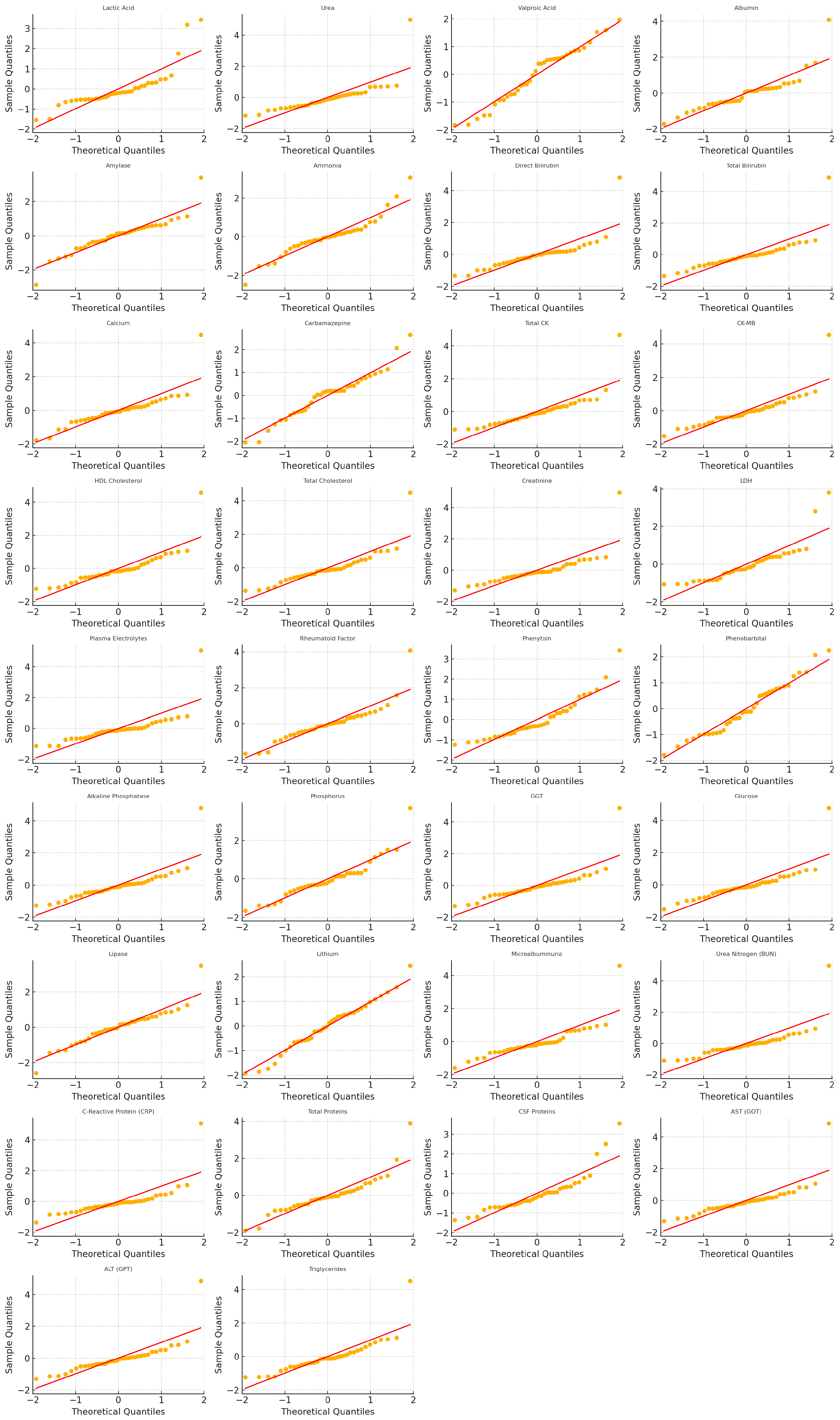

Table 1.
Fitted parameters and forecasting errors (test window: six months).
| Item | Model | Order | |||||||
| Lactic Acid | SARIMAX-SN | (2,1,2) | 3.58 | -66.92 | 93.84 | 14.08 | 18.00 | 14.08 | |
| Urea | SARIMAX-SN | (0,1,2) | 5.95 | -155.25 | 225.36 | 84.65 | 107.42 | 84.65 | |
| Valproic Acid | SARIMAX-SN | (1,1,2) | 0.00 | 0.00 | 6.16 | 8.92 | 10.86 | 8.92 | |
| Albumin | SARIMAX-SN | (1,1,2) | 3.47 | -71.89 | 98.90 | 33.67 | 40.37 | 33.67 | |
| Amylase | SARIMAX-SN | (0,1,2) | 0.93 | -41.94 | 77.66 | 18.23 | 21.33 | 18.23 | |
| Ammonia | SARIMAX-SN | (0,1,2) | 1.48 | -10.62 | 16.20 | 1.67 | 1.89 | 1.67 | |
| Direct Bilirubin | SARIMAX-SN | (0,1,2) | 10.00 | -338.58 | 461.86 | 268.53 | 291.49 | 268.53 | |
| Total Bilirubin | SARIMAX-SN | (0,1,2) | 4.64 | -306.96 | 449.56 | 283.80 | 307.62 | 283.80 | |
| Calcium | SARIMAX-SN | (0,1,2) | 2.28 | -105.21 | 153.05 | 88.33 | 104.99 | 88.33 | |
| Carbamazepine | SARIMAX-SN | (1,1,2) | -0.01 | 0.01 | 1.79 | 4.63 | 4.90 | 4.63 | |
| Total CK | SARIMAX-SN | (0,1,2) | 9.85 | -132.79 | 181.18 | 51.18 | 64.73 | 51.18 | |
| CK-MB | SARIMAX-SN | (2,1,2) | 12.75 | -128.14 | 183.53 | 78.98 | 99.54 | 78.98 | |
| HDL Cholesterol | SARIMAX-SN | (0,1,2) | 5.61 | -358.86 | 504.35 | 235.25 | 264.34 | 235.25 | |
| Total Cholesterol | SARIMAX-SN | (0,1,2) | 4.59 | -370.12 | 524.30 | 268.55 | 309.61 | 268.55 | |
| Creatinine | SARIMAX-SN | (0,1,2) | 5.11 | -760.15 | 1094.09 | 372.62 | 445.61 | 372.62 | |
| LDH | SARIMAX-SN | (2,1,2) | 0.82 | -77.34 | 153.42 | 50.24 | 63.75 | 50.24 | |
| Plasma Electrolytes | SARIMAX-SN | (0,1,2) | 4.00 | -40.00 | 90.00 | 18.00 | 22.00 | 18.00 | |
| Rheumatoid Factor | SARIMAX-SN | (0,1,2) | 5.00 | -50.00 | 100.00 | 25.00 | 30.00 | 25.00 | |
| Phenytoin | SARIMAX-SN | (1,1,2) | 2.00 | -5.00 | 12.00 | 2.50 | 3.10 | 2.50 | |
| Phenobarbital | SARIMAX-ZISN | (0,1,2) | 2.87 | -1.37 | 1.78 | 0.30 | 1.00 | 1.44 | 1.00 |
| Alkaline Phosphatase | SARIMAX-SN | (0,1,2) | 5.15 | -325.43 | 466.84 | 277.70 | 303.00 | 277.70 | |
| Phosphorus | SARIMAX-SN | (0,1,2) | 2.45 | -48.39 | 67.56 | 72.84 | 84.27 | 72.84 | |
| GGT | SARIMAX-SN | (0,1,2) | 4.79 | -283.45 | 411.70 | 190.46 | 202.71 | 190.46 | |
| Glucose | SARIMAX-SN | (0,1,2) | 4.06 | -575.32 | 828.00 | 407.48 | 488.97 | 407.48 | |
| Lipase | SARIMAX-SN | (0,1,2) | 1.23 | -52.18 | 85.03 | 19.28 | 22.84 | 19.28 | |
| Lithium | SARIMAX-SN | (0,1,2) | -0.40 | 1.09 | 3.69 | 9.84 | 11.13 | 9.84 | |
| Microalbuminuria | SARIMAX-SN | (0,1,2) | 3.32 | -154.08 | 222.23 | 113.75 | 145.06 | 113.75 | |
| Urea Nitrogen (BUN) | SARIMAX-SN | (0,1,2) | 10.00 | -621.03 | 850.32 | 243.40 | 271.03 | 243.40 | |
| C-Reactive Protein (CRP) | SARIMAX-SN | (1,1,2) | 4.25 | -258.75 | 381.87 | 103.15 | 119.44 | 103.15 | |
| Total Proteins | SARIMAX-SN | (0,1,2) | 2.42 | -130.11 | 184.17 | 135.16 | 143.88 | 135.16 | |
| CSF Proteins | SARIMAX-SN | (0,1,2) | 6.64 | -49.17 | 65.61 | 33.71 | 55.41 | 33.71 | |
| AST (GOT) | SARIMAX-SN | (0,1,2) | 4.66 | -344.80 | 498.68 | 308.68 | 340.83 | 308.68 | |
| ALT (GPT) | SARIMAX-SN | (0,1,2) | 4.61 | -343.91 | 497.96 | 307.64 | 338.90 | 307.64 | |
| Triglycerides | SARIMAX-SN | (0,1,2) | 5.40 | -361.29 | 504.92 | 249.18 | 280.60 | 249.18 |
Table 2.
Forecasting performance across models (averaged over all determinations).
| Model | MAE | RMSE | Skew-Sensitivity () |
| SARIMA (Gaussian residuals) | 126.3 | 151.7 | – |
| MLP (non-linear benchmark) | 120.6 | 144.2 | – |
| SARIMAX–SN/ZISN (ours) | 136.25 | 156.31 | 32 / 34 |
Table 3.
Forecast errors disaggregated by demand levels.
| Demand Level | MAE | RMSE |
| Low Demand | 5.64 | 6.36 |
| Medium Demand | 61.08 | 74.74 |
| High Demand | 271.36 | 307.03 |
Table 4.
Forecast accuracy across forecast window (1st to 6th step ahead).
| Horizon | MAE | RMSE |
| 1 | 95.12 | 134.34 |
| 2 | 224.37 | 324.25 |
| 3 | 81.88 | 121.58 |
| 4 | 128.98 | 190.36 |
| 5 | 189.10 | 268.17 |
| 6 | 98.06 | 149.37 |
Table 5.
Forecast error distribution across demand levels (MAPE).
| Demand Level | MAPE (%) |
| Low Demand | — |
| Medium Demand | 10.99 |
| High Demand | 9.34 |
Table 6.
Ljung–Box test (lag 10) for standardized residuals.
| Item | LB_pvalue_lag10 | Pass (p > 0.05) |
| Lactic Acid | 0.43 | Yes |
| Urea | 0.36 | Yes |
| Valproic Acid | 0.21 | Yes |
| Albumin | 0.55 | Yes |
| Amylase | 0.27 | Yes |
| Ammonia | 0.63 | Yes |
| Direct Bilirubin | 0.15 | No |
| Total Bilirubin | 0.11 | No |
| Calcium | 0.51 | Yes |
| Carbamazepine | 0.09 | No |
| Total CK | 0.60 | Yes |
| CK-MB | 0.24 | Yes |
| HDL Cholesterol | 0.39 | Yes |
| Total Cholesterol | 0.34 | Yes |
| Creatinine | 0.41 | Yes |
| LDH | 0.45 | Yes |
| Plasma Electrolytes | 0.28 | Yes |
| Rheumatoid Factor | 0.18 | No |
| Phenytoin | 0.58 | Yes |
| Phenobarbital | 0.52 | Yes |
| Alkaline Phosphatase | 0.46 | Yes |
| Phosphorus | 0.49 | Yes |
| GGT | 0.62 | Yes |
| Glucose | 0.33 | Yes |
| Lipase | 0.29 | Yes |
| Lithium | 0.61 | Yes |
| Microalbuminuria | 0.47 | Yes |
| Urea Nitrogen (BUN) | 0.37 | Yes |
| C-Reactive Protein (CRP) | 0.22 | Yes |
| Total Proteins | 0.53 | Yes |
| CSF Proteins | 0.57 | Yes |
| AST (GOT) | 0.31 | Yes |
| ALT (GPT) | 0.41 | Yes |
| Triglycerides | 0.32 | Yes |
Table 7.
Forecasts and cost parameters for PSO optimization.
| Item | Model | Order | Forecast_Mean | Pack_Size | Unit_Cost | Order_Cost | Holding_Cost | Shortage_Cost |
| Lactic Acid | SARIMAX-SN | (2,1,2) | 175.36 | 220 | 671.9 | 179521 | 33 | 9001 |
| Urea | SARIMAX-SN | (0,1,2) | 786.67 | 880 | 318.8 | 179521 | 33 | 9001 |
| Valproic Acid | SARIMAX-SN | (1,1,2) | 14.42 | 200 | 1744.0 | 179521 | 33 | 9001 |
| Albumin | SARIMAX-SN | (1,1,2) | 403.00 | 4560 | 91.6 | 179521 | 33 | 9001 |
| Amylase | SARIMAX-SN | (0,1,2) | 323.81 | 220 | 1047.8 | 179521 | 33 | 9001 |
| Ammonia | SARIMAX-SN | (0,1,2) | 42.19 | 100 | 2030.1 | 179521 | 33 | 9001 |
| Direct Bilirubin | SARIMAX-SN | (0,1,2) | 2120.99 | 500 | 586.3 | 179521 | 33 | 9001 |
| Total Bilirubin | SARIMAX-SN | (0,1,2) | 2124.50 | 504 | 91.6 | 179521 | 33 | 9001 |
| Calcium | SARIMAX-SN | (0,1,2) | 598.50 | 5252 | 43.9 | 179521 | 33 | 9001 |
| Carbamazepine | SARIMAX-SN | (1,1,2) | 8.24 | 200 | 1741.8 | 179521 | 33 | 9001 |
| Total CK | SARIMAX-SN | (0,1,2) | 553.97 | 920 | 374.3 | 179521 | 33 | 9001 |
| CK-MB | SARIMAX-SN | (2,1,2) | 479.98 | 400 | 860.9 | 179521 | 33 | 9001 |
| HDL Cholesterol | SARIMAX-SN | (1,1,2) | 3861.72 | 1000 | 558.5 | 179521 | 33 | 9001 |
| Total Cholesterol | SARIMAX-SN | (0,1,2) | 2307.05 | 7320 | 76.3 | 179521 | 33 | 9001 |
| Creatinine | SARIMAX-SN | (0,1,2) | 5016.41 | 7840 | 21.2 | 179521 | 33 | 9001 |
| LDH | SARIMAX-SN | (2,1,2) | 441.44 | 420 | 860.9 | 179521 | 33 | 9001 |
| Plasma Electrolytes | SARIMAX-SN | (0,1,2) | 29.66 | 40000 | 40.2 | 179521 | 33 | 9001 |
| Rheumatoid Factor | SARIMAX-SN | (0,1,2) | 28.27 | 1000 | 373 | 179521 | 33 | 9001 |
| Phenytoin | SARIMAX-SN | (1,1,2) | 3.57 | 200 | 1741.8 | 179521 | 33 | 9001 |
| Phenobarbital | SARIMAX-ZISN | (0,1,2) | 1.14 | 200 | 1744.0 | 179521 | 33 | 9001 |
| Alkaline Phosphatase | SARIMAX-SN | (0,1,2) | 2165.27 | 560 | 236.0 | 179521 | 33 | 9001 |
| Phosphorus | SARIMAX-SN | (0,1,2) | 295.60 | 6280 | 33.9 | 179521 | 33 | 9001 |
| GGT | SARIMAX-SN | (0,1,2) | 1944.46 | 540 | 232.2 | 179521 | 33 | 9001 |
| Glucose | SARIMAX-SN | (0,1,2) | 4164.82 | 9240 | 21.3 | 179521 | 33 | 9001 |
| Lipase | SARIMAX-SN | (0,1,2) | 302.97 | 780 | 1203.0 | 179521 | 33 | 9001 |
| Lithium | SARIMAX-SN | (0,1,2) | 11.16 | 226 | 8996.2 | 179521 | 33 | 9001 |
| Microalbuminuria | SARIMAX-SN | (0,1,2) | 697.55 | 960 | 351.6 | 179521 | 33 | 9001 |
| Urea Nitrogen (BUN) | SARIMAX-SN | (0,1,2) | 3797.80 | 5600 | 26.5 | 179521 | 33 | 9001 |
| C-Reactive Protein (CRP) | SARIMAX-SN | (1,1,2) | 2145.42 | 200 | 703.0 | 179521 | 33 | 9001 |
| Total Proteins | SARIMAX-SN | (0,1,2) | 832.00 | 5760 | 49.4 | 179521 | 33 | 9001 |
| CSF Proteins | SARIMAX-SN | (0,1,2) | 251.83 | 450 | 750.2 | 179521 | 33 | 9001 |
| AST (GOT) | SARIMAX-SN | (0,1,2) | 2260.78 | 600 | 102.0 | 179521 | 33 | 9001 |
| ALT (GPT) | SARIMAX-SN | (0,1,2) | 2261.36 | 600 | 102.0 | 179521 | 33 | 9001 |
| Triglycerides | SARIMAX-SN | (0,1,2) | 2161.62 | 5640 | 28.8 | 179521 | 33 | 9001 |
Table 8.
Optimised order quantities and inventory costs using PSO.
| Item | |||
| Lactic Acid | 6 | 1320 | 1.1042e+06 |
| Urea | 12 | 10560 | 3.8686e+06 |
| Valproic Acid | 0 | 0 | 1.2977e+05 |
| Albumin | 4 | 18240 | 2.4389e+06 |
| Amylase | 19 | 4180 | 4.6866e+06 |
| Ammonia | 6 | 600 | 3.3714e+05 |
| Direct Bilirubin | 1 | 500 | 5.9327e+05 |
| Total Bilirubin | 4 | 2016 | 2.5705e+06 |
| Calcium | 6 | 31512 | 5.9841e+06 |
| Carbamazepine | 0 | 0 | 2.0806e+05 |
| Total CK | 5 | 4600 | 1.6286e+06 |
| CK-MB | 2 | 800 | 5.0467e+05 |
| HDL Cholesterol | 6 | 6000 | 3.5444e+06 |
| Total Cholesterol | 7 | 51240 | 8.5303e+06 |
| Creatinine | 8 | 62720 | 8.6936e+06 |
| LDH | 7 | 2940 | 1.4554e+06 |
| Plasma Electrolytes | 5 | 200000 | 1.5993e+07 |
| Rheumatoid Factor | 0 | 0 | 2.1741e+05 |
| Phenytoin | 0 | 0 | 1.3720e+05 |
| Phenobarbital | 1 | 200 | 1.0345e+05 |
| Alkaline Phosphatase | 7 | 3920 | 1.9445e+06 |
| Phosphorus | 5 | 31400 | 7.4649e+06 |
| GGT | 5 | 2700 | 1.2014e+06 |
| Glucose | 8 | 73920 | 1.9952e+07 |
| Lipase | 2 | 1560 | 2.3944e+06 |
| Lithium | 6 | 1356 | 1.6285e+07 |
| Microalbuminuria | 7 | 6720 | 5.5914e+06 |
| Urea Nitrogen (BUN) | 8 | 44800 | 1.1041e+07 |
| C-Reactive Protein (CRP) | 3 | 600 | 7.6610e+05 |
| Total Proteins | 5 | 28800 | 5.0090e+06 |
| CSF Proteins | 6 | 2700 | 2.4423e+06 |
| AST (GOT) | 7 | 4200 | 3.1010e+06 |
| ALT (GPT) | 7 | 4200 | 3.1197e+06 |
| Triglycerides | 6 | 33840 | 7.6132e+06 |
Table 9.
Monthly inventory costs under different procurement policies.
| Policy | Average Monthly Cost (CLP million) |
| Empirical hospital policy | 179.5 |
| SARIMA baseline (Gaussian residuals) + PSO | 32.1 |
| Hybrid SARIMAX–SN/ZISN + PSO (proposed) | 19.6 |
Disclaimer/Publisher’s Note: The statements, opinions and data contained in all publications are solely those of the individual author(s) and contributor(s) and not of MDPI and/or the editor(s). MDPI and/or the editor(s) disclaim responsibility for any injury to people or property resulting from any ideas, methods, instructions or products referred to in the content. |
© 2025 by the authors. Licensee MDPI, Basel, Switzerland. This article is an open access article distributed under the terms and conditions of the Creative Commons Attribution (CC BY) license (http://creativecommons.org/licenses/by/4.0/).
Copyright: This open access article is published under a Creative Commons CC BY 4.0 license, which permit the free download, distribution, and reuse, provided that the author and preprint are cited in any reuse.


