Submitted:
23 July 2025
Posted:
23 July 2025
You are already at the latest version
Abstract
Life tables and survival analysis are crucial statistical tools that have been widely applied in various areas of research, particularly in medicine and clinical studies. They help predict survival probabilities over time as well as assess the impact of covariates on survival outcomes. In the present paper, the utility of both life tables and Kaplan-Meier survival analysis to research in the social sciences is illustrated, with particular emphasis placed on their usefulness in analyses involving “censored” data as well as on their relatively straightforward application within the SPSS statistical software program. Additionally, it covers the premises, applications, and benefits of each of these statistical methods for analyzing time-to-event data. It goes on to provide examples of how these might be utilized for medical conditions, including brain tumors, liver cancer, and lung cancer. The paper concludes by highlighting the importance of life tables and survival analysis in medicine, providing insights into survival rates and treatment efficacy.
Keywords:
Life Tables
; Survival Analysis
; Kaplan-Meier
; Censored Data
; Medical Research
; Time-to-Event Data
1. Introduction
The notion of time to some event, for example, death, progression, or recovery from disease, is fundamental to medical and clinical research. These studies can more commonly be classified as studies of time-to-event data, in which the main interest is how long it takes for an event to occur. Two prevalent statistical approaches that have sought to deal with this type of data are life tables and survival analysis. These methods are particularly helpful when not all subjects in the study experience the event of interest during the study period, resulting in censored cases [1,2,3].
A case is considered censored if the outcome of interest has not been observed until the time of the study [4]. This may be the case when the subject is alive after the study or withdraws for reasons that are unrelated to the event of interest. These scenarios run into issues with common statistical methods like t-tests or linear regression that assume a complete data set for their cases. To accommodate this problem, Lifetables and the Kaplan-Meier technique for the analysis of survival have been developed, which are useful tools to handle “censored” data and yield valid point estimates of survival proportions at specified points in time [5,6,7,8].
Life tables discretize the observation period into small time intervals and estimate the probability of experiencing the event in each time interval [9,10]. These are assumed to be intervals in which the probability of an event occurring at any given point within the interval is assumed to be constant among those living in that interval [11]. Conversely, the non-parametric Kaplan-Meier survival analysis does not assume a constant probability of events within time intervals and thus estimates the survival function. This technique is especially useful in cases of smaller sample sizes and sparse data points [12,13].
The purpose of this paper is to touch on the theory and applications of the life table and the Kaplan-Meier survival figure, along with points of interest in their use in medicine [14]. We will see how these techniques lend themselves to estimates of survival probabilities and hazard rates as well as comparisons of treatment or patient sub-groups. In addition, we are going to show how these techniques can be applied using SPSS software as a practical tool for data analysis [15,16,17,18].
Life tables and Kaplan-Meier analysis allow physicians to determine treatment as well as prognosis. These methods enable a more explicit interpretation of survival patterns, which in turn assist physicians and clinicians in determining optimal care for patients [19,20]. Life tables, which display survival of patients on different treatments, and Kaplan-Meier survival curves that graphically depict survival probabilities and lend themselves more readily to comparisons between groups, for instance, are examples of these techniques [21].
Such analyses can only take place in medicine, for instance, in clinical trials where an experiment is conducted to verify the efficacy of a novel treatment or medication. Similarly, in the study of cancer, life tables and the Kaplan-Meier analyses are utilized to assess the efficacy of a new chemotherapy treatment by ascertaining whether patients on the experimental treatment survive longer than patients on conventional chemotherapy [22,23]. Though these may also serve in the assessment of the influence of additional factors such as age, gender, or comorbidities on survival.
Important assumptions of these kinds of statistics will also be covered here, such as the proportional hazard assumption of the Kaplan-Meier analyses and the independence of censoring, and the event. It will discuss how these assumptions affect the analysis and later provide a set of recommendations for “good” survival analysis [24,25].
2. Literature Review
2.1. Life Tables and Survival Analysis
Life tables provide a statistical representation of the time until the event, generally survival, in each population [26]. The idea behind life tables is to partition the period of observation into smaller intervals of time and to estimate the probability of the event of interest occurring in each of the intervals. This is advantageous, particularly in the case of censored data, as it allows the estimation of survival probabilities at multiple points in time. Among them, Kaplan and Meier posed several statistical solutions to help the work of survival data analysis, including Kaplan-Meier survival analysis and Cox regression [27,28].
The Kaplan-Meier survival analysis is a method for estimating the survival function based on life tables. This is often used in clinical trials to compare survival probabilities between groups. The Cox regression is instead a semi-parametric method able to include covariates that allows for studying the effect of other variables on the survival time (Cox 1972) [2].
Kaplan and Meier’s seminal work introduced the Kaplan-Meier estimator, a non-parametric method used to estimate survival functions from time-to-event data. This method is particularly, but perhaps more useful, when some of the observations are censored [29]. The Kaplan-Meier estimator estimates survival probabilities at each event time based on the number at risk and the number experiencing the event [30]. This work was the basis for much of the modern survival analysis and is common practice in medical research to estimate survival probabilities for patients within clinical trials [31].
The Cox regression model examines the effect of covariates on survival time and was introduced in Cox’s paper on proportional hazards models [32]. Because it does not make a specified assumption regarding the form of the baseline hazard function, the model is semi-parametric and is considered a semi-parametric approach to survival analysis. Cox survival analysis is a frequently utilized statistical tool in clinical studies to analyze the impact of covariates, such as treatment or patient characteristics, on the time until an event occurs for a subject. Survival analyses using this approach are frequently completed alongside life tables and Kaplan-Meier analyses [33,34].
The book by Klein and Moesch Berger details all the survival analysis methods, including life tables, Kaplan-Meier analysis, and Cox regression. It encompasses the full spectrum of techniques for dealing with the analysis of censored and truncated data within the fields of Biostatistics, Medicine, Engineering, and the Social Sciences. The second edition provides enhanced discussion of these approaches in applied research with many examples, including those from cancer and cardiovascular research [35]. The book is a complete guide for someone new to survival analysis as well as for someone more experienced with it.
Breslow’s contribution can be seen as an alternative to Cox regression as a means of dealing with covariates in the presence of censored survival data. His method, Breslow’s approximation, is one way to obtain parameter estimates for the case of tied event times in survival analysis [36,37,38,39,40]. This approach is commonly employed in medical research because tied event times are frequent in time-to-event data, particularly in the case of small clinical trials where patients or events are few [41,42].
This Paper serves as a practical starting point for applying survival analysis, particularly regression models, to time-to-event data. It covers life tables, Kaplan-Meier estimates, and the Cox proportional hazards model in depth. In addition to the methods, they discuss the underlying assumptions and offer guidance on utilizing these techniques for practical medical problems, like the survival of patients following surgery or the effect of treatment protocols on the course of a disease [43,44,45].
The book by Armitage and Berry is a definitive work on the application of statistics to medical research and discusses many statistical techniques, including survival analysis [46]. The third edition also has complete sections on life table techniques, Kaplan-Meier analysis, and the more complicated topic of survival data regression modeling [47,48]. They also include practical examples and case studies from clinical trials to show the use of these kinds of methods in medical research [49].
Therneau and Grambsch offer a broader extension of Cox’s regression model to incorporate complex survival data that includes time-dependent covariates and the interaction of covariates [50]. They are likely to become an important resource for anyone who must contend with this type of survival data. The usefulness of this book is particularly relevant in clinical trials in which the treatment effect is time-varying [51,52,53,54].
2.2. Applications in Medical and Clinical Research
Survival analysis and life tables have been extensively employed in medical and clinical studies. These techniques have been frequently applied to determine treatment efficacy, prognostic indications of disease, and risk factor survival analyses. Life tables are employed in fields such as cancer studies, where survival rates for patients receiving different therapies are analyzed. Likewise, survival analysis is used in cardiovascular studies to recognize predictors of longer or shorter survival following heart attacks or surgeries [55,56].
3. Methodology
The statistical procedures utilized in this paper are life table analysis and the Kaplan-Meier survival analysis [57]. LTA uses the actuarial, or lifetable, approach, which partitions the observation period into smaller time intervals for the determination of event occurrence probability within each interval. The Kaplan-Meier method is a non-parametric approach that constructs an estimate of the survival function from the actual times of observed events [58,59].
Data for the analysis is obtained from medical studies involving patients with various conditions, such as brain tumors, liver cancer, and lung cancer. SPSS software is used to perform the analysis, where variables such as survival time, event status (death or survival), and treatment type are considered [60,61,62,63,64].
3.1. Assumptions
- The probability of the event of interest depends only on the time after the initial event.
- The survival function is assumed to be stable over time.
- There are no systematic differences between censored and non-censored cases.
4. Application
To compare two groups of (20) patients with a brain tumor, one of them received treatment A (Group 1) or conventional medication, while the second group received treatment B (Group 2) the new medication through the formation of a life table (Life Table) for a period measured in weeks and the event is the death of the Patient (1) while his survival (0).
The life schedule is analyzed in some steps. We get Table 1 results.
A life schedule is a descriptive table that summarizes the time it takes for an event to occur. The table is divided by each group (here we have two groups), including the period (0-30) as determined by the highest value (30), which has a Category length of 5. Then, determine the number of entrants in the corresponding period. Or the number of surviving cases at the beginning of the period. This value decreases steadily with each period as people who have died and for both groups. Here we have (20) people for the first group at the beginning of the study, of whom (8) died for the period from zero to less than (5) and of whom (12) survived, while one person from the second group, which reached (20) people also died, of whom (19) people remained, and so on, the rest of the values reach (3) survivors for the first group and(6) for the second group at the end of the study (30).
And determine the number of controlled cases in this period. These are still alive, but so far they have not existed longer than the indicated period in period. And here, there is only one person who survived outside the study for the period (15-20).
The table also shows that the greatest number and percentage of terminal events occurred during the first period (for the first group), with the highest risk rate, which indicates that patients should be closely monitored during the first period of the first group for their safety.
The median survival time (in Table 2) shows that the second group (who received the new drug) had an average survival time equal to 19.79 weeks and was better than the first group (who received the traditional drug) by an average of 10 weeks.
Survival curves give a visual representation of life schedules (Figure 1). The horizontal axis shows the time of the event. In this figure, the decreases in the survival curve occur at 5-week intervals, as specified in the previous dialog box. The vertical axis shows the probability of survival. Thus, any point on the survival curve shows the probability that the patient will remain in a certain category after that time.
It seems that the patients of the first group have a lower survival curve than the second group, and this is confirmed by the following risk function in Figure 2:
To determine whether these differences are due to chance, look at the tables of comparisons.
Table 3 provides a comprehensive test of the evenness of survival times across groups. The test statistics are based on the differences in the scores of the average group. Roughly speaking, the individual degree of the condition is increased for each comparison in which the survival time is higher and decreases when it has a lower survival time. The average score for the group is the average of the individual scores of the cases in the group. Since the value of p is greater than the morale level (0.05) of the Wilcoxon test (Jehan), you can conclude that the survival curves of the two groups do not differ significantly.
Kaplan-Meier Survival Analysis (Kaplan-Meier Survival Analysis):
There are several situations in which you may want to examine the distribution of times between two events, such as the length of employment (the time between hiring and leaving the company). However, this type of data usually includes some controlled cases. Controlled cases are cases where the second event was not recorded (for example, people were still working for the company at the end of the study). The Kaplan-Meier procedure is a method for estimating time-to-event models in the presence of controlled situations. The Kaplan-Meier model is based on estimating the conditional probabilities at each point in time when an event occurs and taking the resulting target (Limit) of these probabilities to estimate the survival rate at each point in time. For example, does the new AIDS treatment have any therapeutic benefit in prolonging life? You can conduct a study using two groups of AIDS patients, one receiving conventional treatment and the other receiving experimental treatment. The construction of the Kaplan-Meier model from the data will allow you to compare the overall survival rates between the two groups to determine whether the experimental treatment represents an improvement over conventional treatment. Kaplan Meier uses and Assumptions (Kaplan-Meier uses and Assumptions):
The Kaplan-Meier procedure uses a method for calculating life tables that estimate the survival or risk function at the time of each event. The life tables procedure uses an actuarial approach to survival analysis based on dividing the observation period into smaller time intervals and may be useful for dealing with large samples. Kaplan-Meier survival analysis is a descriptive procedure for examining the distribution of time variables to an event. In addition, you can compare the distribution by levels of the factor variable, or the product of separate analyses by levels of the stratification variable.
Assumptions: the probabilities for the event of interest should depend only on the time after the initial event - they are assumed to be stable concerning (positive) time. That is, cases entering the study at different times (for example, patients starting treatment at different times) should behave similarly. There should also be no stereotypical differences between controlled and uncontrolled cases. If many of the controlled cases are, for example, patients with more serious conditions, then your results may be biased. Let's get the following results:
The summary Table 4 of the case Operations shows that there were (40) sightings distributed over two groups of (20) sightings for which the first group took conventional treatment (17) event cases (death) versus (3) surviving cases, while the second group took suggested treatment for (13) death versus (7) surviving cases.
The survival schedule is a descriptive Table 5, separating the time until the drug takes effect. The table is divided by each level of treatment, and each viewing takes its row in the table. As a result, the table is quite large. Time represents the time of occurrence of the event or control.
Status indicates whether the status has been subjected to the final event or has been censored.
Cumulative Proportion Surviving at the time: the cumulative percentage surviving at that time, that is, the percentage of cases that survived from the beginning of the table to this time. When multiple cases experience the final event at the same time, these estimates are calculated once for that period and apply to all cases where the drug has become effective at that time, with the standard error.
N of Cumulative Events: the number of cumulative events, that is, the number of cases that have gone through the experience of the event from the beginning of the table to this time.
N of Remaining Cases: the number of remaining cases, that is, the number of cases that at this time have not witnessed the final event or were not controlled.
Table 6 of survival averages and medians provides a quick numerical comparison of the "typical" Times of impact for both conventional treatments, proposed, and total. Since there is a lot of overlap in confidence intervals, it is unlikely that there will be a significant (or significant) difference in the "average" survival time.
Table 7 presents the three comprehensive tests for the equalization of survival times across groups. Since the values of the tests of the teams are all greater than the morale level of 0.05, it is not possible to determine a significant difference between the survival curve of the first group compared with the second, as in Figure 3.
The survival curves give a visual representation of the life tables; the horizontal axis shows the time of the event. in this figure, we observe a decrease in the survival curve when the drug is applied to the patient. The vertical axis shows the probability of survival. And therefore, any point on the survival curve shows the probability that the patient undergoing the appointed treatment will not feel comfortable by that time. The curve of the new drug is much steeper than the current one throughout most of the trial period, suggesting that the new drug may give an advantage over the old one. To determine whether these differences are due to chance and the results of which cannot be generalized, look at the table of comparisons.
Using the Kaplan-Meier survival analysis procedure, the time distribution of the effect of two different drugs was tested, and comparative tests show that there is no statistically significant difference between them. We also note that the cumulative hazard function curve for the new drug group was lower than the cumulative hazard function curve for the traditional drug group, as shown in Figure 4:
5. Results
The analysis of life table data reveals the survival rates of patients undergoing different treatments. In the case of brain tumor patients, the group receiving the new treatment showed significantly higher survival rates compared to those receiving conventional treatment. Kaplan-Meier survival curves further illustrate the differences in survival probabilities between the two groups, with the new treatment group demonstrating a more favorable survival profile, as in Table 8.
6. Discussion
The outcomes of the survival analysis, including life tables and Kaplan-Meier survival analysis, suggest that these methods can be used to assess survival between treatment groups. The life table technique is less precise, can only be used if none of the subjects are censored, and the Kaplan-Meier procedure can accurately estimate the survival function at all time points. These methods are particularly useful to medical research, since censored data are common in medicine, and survival predictions often play an important role in treatment decisions.
Survival probabilities and hazard rates are quite valid, and it is easy to carry out these analyses with SPSS. It highlights the need to know what implicit assumptions are made under possible analytic methods for interpretations to be valid.
7. Conclusion
Life tables and survival analysis represent perhaps the best-known approaches to the description of time- until- event data, particularly in clinical and medical research. These techniques allow the incorporation of censored cases in the analysis, the estimation of survival probability estimates, as well as the testing of covariate effects on survival. These methods are easily conducted within SPSS, which is accessible to many more researchers than those with specialized software, and they yield valuable information regarding treatment response and disease prognosis.
Future Directions: Cox regression could be used to assess the influence of several covariates on survival in future research. Also, the use of time-dependent covariates could improve the models of survival analysis when the environment is dynamic.
References
- Kaplan, E. L., & Meier, P. (1958). Nonparametric Estimation from Incomplete Observations. Journal of the American Statistical Association, 53(282), 457-481. [CrossRef]
- Cox, D. R. (1972). Regression Models and Life Tables. Journal of the Royal Statistical Society: Series B (Methodological), 34(2), 187-220. [CrossRef]
- Klein, J. P., & Moeschberger, M. L. (2003). Survival Analysis: Techniques for Censored and Truncated Data (2nd ed.). Springer. [CrossRef]
- Collett, D. (2015). Modelling Survival Data in Medical Research (3rd ed.). CRC Press. [CrossRef]
- Breslow, N. E. (1974). Covariance Analysis of Censored Survival Data. Biometrics, 30(1), 89-99. [CrossRef]
- Hosmer, D. W., & Lemeshow, S. (1999). Applied Survival Analysis: Regression Modeling of Time-to-Event Data. Wiley-Interscience.
- Armitage, P., & Berry, G. (1994). Statistical Methods in Medical Research (3rd ed.). Blackwell Science.
- Therneau, T. M., & Grambsch, P. M. (2000). Modeling Survival Data: Extending the Cox Model. Springer. [CrossRef]
- Ali, T. H. (2022). Modification of the adaptive Nadaraya-Watson kernel method for nonparametric regression (simulation study). Communications in Statistics - Simulation and Computation, 51(2), 391–403. [CrossRef]
- Ali, Taha Hussein, Heyam Abd Al-Majeed Hayawi, and Delshad Shaker Ismael Botani. "Estimation of the bandwidth parameter in Nadaraya-Watson kernel non-parametric regression based on universal threshold level." Communications in Statistics-Simulation and Computation 52.4 (2023): 1476-1489. [CrossRef]
- Ali, Taha Hussein, Saman Hussein Mahmood, and Awat Sirdar Wahdi. "Using Proposed Hybrid method for neural networks and wavelet to estimate time series model." Tikrit Journal of Administration and Economics Sciences 18.57 part 3 (2022). https://www.tjaes.org/index.php/tjaes/article/view/324. [CrossRef]
- Heyam A. Hayawi, Ahmed Mahmoud Al-Sabawi,(2002),”methods”, The third Scientific Conference of the Iraqi society for Statistical Sciences,182-199.
- Heyam A. Hayawi, Ahmed Mahmoud Al-Sabawi,(2002),”A proposed Method for Solving the Transportation Model”,Iraqi Journal Of Statistical Sciences, 4 (2), 61-71.
- Ali, Taha Hussein and Jwana Rostam Qadir. "Using Wavelet Shrinkage in the Cox Proportional Hazards Regression model (simulation study)", Iraqi Journal of Statistical Sciences, 19, 1, 2022, 17-29. https://stats.uomosul.edu.iq/article_174328.html. [CrossRef]
- Ali, Taha Hussein, and Saleh, Dlshad Mahmood, "Proposed Hybrid Method for Wavelet Shrinkage with Robust Multiple Linear Regression Model: With Simulation Study" QALAAI ZANIST JOURNAL 7.1 (2022): 920-937. https://journal.lfu.edu.krd/ojs/index.php /qzj/article/view/907/937. [CrossRef]
- Ali, Taha Hussein, and Dlshad Mahmood Saleh. "COMPARISON BETWEEN WAVELET BAYESIAN AND BAYESIAN ESTIMATORS TO REMEDY CONTAMINATION IN LINEAR REGRESSION MODEL" PalArch's Journal of Archaeology of Egypt/Egyptology 18.10 (2021): 3388-3409. https://www.archives.palarch.nl/index.php/ja e/article/view/10382/9524.
- Ali, Taha Hussein, Rahim, Alan Ghafur, and Saleh, Dlshad Mahmood. "Construction of Bivariate F-Control Chart with Application" EURASIAN JOURNAL OF SCIENCE AND ENGINEERING (EAJSE), 4.2 (2018): 116-133. [CrossRef]
- Taha H. A., Dr.Nazeera Sedeek K., and Awaz Shahab Mohammad "Construction robust simple linear regression profile Monitoring" Journal of Kirkuk University for Administrative and Economic Sciences, 9.1. (2019): 242-257. https://iasj.rdd.edu.iq/journals/uploads /2024/12/07/30d2a37cb5b86ed8c2079a73e2818afc.pdf.
- Omar, C., Ali, T. H., & Hassn, K. (2020). Using Bayes weights to remedy the heterogeneity problem of random error variance in linear models. Iraqi Journal of Statistical Sciences, 17(2), 58–67. https://stats.uomosul.edu.iq/article_167391_002eac088c04564fa24970cc53dc749d.pdf. [CrossRef]
- Qais Mustafa Abd alqader and Taha Hussien Ali, (2020), Monthly Forecasting of Water Consumption in Erbil City Using a Proposed Method, Al-Atroha journal, 5.3:47-67. https://www.researchgate.net/publication/353033062_Monthly_Forecasting_of_Water_Consumption_in_Erbil_City_Using_a_Proposed_Method.
- Ali, Taha Hussein, 2018, Solving Multi-collinearity Problem by Ridge and Eigenvalue Regression with Simulation, Journal of Humanity Sciences, 22.5: 262-276. https://pdfs.semanticscholar.org/77aa/9ef17d35c6cedd2401eaa725f92b18648177.pdf. [CrossRef]
- Ali, Taha Hussein, Nasradeen Haj Salih Albarwari, and Diyar Lazgeen Ramadhan. "Using the hybrid proposed method for Quantile Regression and Multivariate Wavelet in estimating the linear model parameters." Iraqi Journal of Statistical Sciences 20.1 (2023): 9-24. https://stats.uomosul.edu.iq/article_178679.html. [CrossRef]
- Ali, Taha Hussein, Avan Al-Saffar, and Sarbast Saeed Ismael. "Using Bayes weights to estimate parameters of a Gamma Regression model." Iraqi Journal of Statistical Sciences 20.1 (2023): 43-54.https://stats.uomosul.edu.iq/article_178687.html. [CrossRef]
- Raza, Mahdi Saber, Taha Hussein Ali, and Tara Ahmed Hassan. "Using Mixed Distribution for Gamma and Exponential to Estimate of Survival Function (Brain Stroke)." Polytechnic Journal 8.1 (2018). [CrossRef]
- Ali, Taha Hussein & Mardin Samir Ali. "Analysis of Some Linear Dynamic Systems with Bivariate Wavelets" Iraqi Journal of Statistical Sciences 16.3 (2019): 85-109. https://stats.uomosul.edu.iq/article_164176.html. [CrossRef]
- Ali, T. H., Sedeeq, B. S., Saleh, D. M., & Rahim, A. G. (2024). Robust multivariate quality control charts for enhanced variability monitoring. Quality and Reliability Engineering International, 40(3), 1369-1381. [CrossRef]
- Haydier, Esraa Awni, Nasradeen Haj Salih Albarwari, and Ali, Taha Hussein "The Comparison Between VAR and ARIMAX Time Series Models in Forecasting." Iraqi Journal of Statistical Sciences 20.2 (2023): 249- 262. https://stats.uomosul.edu.iq/article_181260 _ff0164e286f99f8046e2ee21368235b4.pdf. [CrossRef]
- Ali, Taha Hussein, Haider, Israa Awni, and Rasoul, Fatima Othman Hama. “Create a Bayesian panel for the number of weighted defects and compare it with the Shewart panel”. Journal of Business Economics for Applied Research, 5.5 (2023): 305-320. https://iasj.rdd.edu.iq/journals/uploads/2024/12/07/a2d11f761ef87ac4b48e1eb942d6049a.pdf. [CrossRef]
- Omer, A. W., Sedeeq, B. S., & Ali, T. H. (2024). A proposed hybrid method for Multivariate Linear Regression Model and Multivariate Wavelets (Simulation study). Polytechnic Journal of Humanities and Social Sciences, 5(1), 112-124. https://journals.epu.edu.iq/index.php /Mitanni/article/view/1452. [CrossRef]
- Samad Sedeeq, B., Muhammad, Z. A., Ali, I. M., & Ali, T. H. (2024). Construction Robust -Chart and Compare it with Hotelling’s T2-Chart. Zanco Journal of Human Sciences, 28(1), 140–157. https://doi.org/10.21271/zjhs.28.1.11. [CrossRef]
- Sakar Ali Jalal; Dlshad Mahmood Saleh; Bekhal Samad Sedeeq; Taha Hussein Ali. "Construction of the Daubechies Wavelet Chart for Quality Control of the Single Value". IRAQI JOURNAL OF STATISTICAL SCIENCES, 21, 1, 2024, 160-169. [CrossRef]
- Ali, T. H., Raza, M. S., & Abdulqader, Q. M. (2024). VAR TIME SERIES ANALYSIS USING WAVELET SHRINKAGE WITH APPLICATION. Science Journal of University of Zakho, 12(3), 345–355. [CrossRef]
- Duaa Faiz Abdullah Faiz Abdullah; Jwana Rostom Qadir; Diyar Lazgeen Ramadhan; Taha Hussein Ali. "CUSUM Control Chart for Symlets Wavelet to Monitor Production Process Quality.". IRAQI JOURNAL OF STATISTICAL SCIENCES, 21, 2, 2024, 54-63. https://iasj.rdd.edu.iq/journals/uploads/2024/12/08/f3592dd1129053cfe9fc12136e50cab2.pdf. [CrossRef]
- Ali, T. H., Saleh, D., Mustafa Abdulqader, Q., & Omer Ahmed, A. (2025). Comparing Methods for Estimating Gamma Distribution Parameters with Outliers Observation. Journal of Economics and Administrative Sciences, 31(145), 163-174. [CrossRef]
- Omer, A. W., & Ali, T. H. (2025). Dealing with the Outlier Problem in Multivariate Linear Regression Analysis Using the Hampel Filter. Kurdistan Journal of Applied Research, 10(1). [CrossRef]
- Elias, I. I., & Ali, T. H. (2025). Optimal level and order of the Coiflets wavelet in the VAR time series denoise analysis. Frontiers in Applied Mathematics and Statistics, 11, 1526540. [CrossRef]
- Elias, Intisar and Hussein Ali, T. (2025) “Choosing an Appropriate Wavelet for VARX Time Series Model Analysis”, Journal of Economics and Administrative Sciences, 31(146), pp. 174–196. https://jeasiq.uobaghdad.edu.iq/index.php/JEASIQ/article/view/3609. [CrossRef]
- Ali, T. H., Hamad, A. A., Mahmood, S. H., & Ahmed, K. H. (2025). ARIMAX time series analysis for a general budget in the Kurdistan Region of Iraq using wavelet shrinkage. Communications in Statistics: Case Studies, Data Analysis and Applications, 11(2), 164–188. [CrossRef]
- Taha Hussein Ali, Hutheyfa Hazem Taha, Mahdi Saber Raza Shalee et al. Evaluating the Effectiveness of Classical and Bayesian Control Charts in Detecting Process Mean Shifts, 28 April 2025, PREPRINT (Version 1) available at Research Square [https://doi.org/10.21203/rs.3.rs-6536864/v1]. [CrossRef]
- Taha Huseeian Ali; Heyam A.A Hayawi; Hunar Adam Hamza. "Bayesian Time Series Modelling with Wavelet Analysis for Forecasting Monthly Inflation". IRAQI JOURNAL OF STATISTICAL SCIENCES, 22, 1, 2025, 181-194. [CrossRef]
- Mahammad Mahmoud Bazid; Taha Hussien Ali. "Estimating Outliers Using the Iterative Method in Partial Least Squares Regression Analysis for Linear Models.". IRAQI JOURNAL OF STATISTICAL SCIENCES, 22, 1, 2025, 88-100. [CrossRef]
- Sarah Bahrooz Ameen; Taha Hussein Ali. "Proposed Quality Control Charts Using Haar Wavelet Coefficients for Enhanced Production Monitoring". IRAQI JOURNAL OF STATISTICAL SCIENCES, 22, 1, 2025, 127-140. [CrossRef]
- Hutheyfa Hazem Taha, Taha Hussein Ali, Heyam A. A. Hayawi et al. Mitigating Contamination Effects on Gamma Distribution Parameter Estimation Using Wavelet Shrinkage Techniques, 10 June 2025, PREPRINT (Version 1) available at Research Square [https://doi.org/10.21203/rs.3.rs-6855768/v1]. [CrossRef]
- Botani, D., Kareem, N., Ali, T., Sedeeq, B. (2025). Optimizing bandwidth parameter estimation for non-parametric regression using fixed-form threshold with Dmey and Coiflet wavelets. Hacettepe Journal of Mathematics and Statistics, 54(3), 1094-1106. [CrossRef]
- Heyam A. Hayawi, Safa Younes Safawi,(2002),”A proposed method for generalizing the optimal state of the boundaries of layers in the stratigraphic preview” ,Iraqi Journal Of Statistical Sciences 3 (2), 37-43.
- Heyam A. Hayawi,(2008),”State Space Models Employment and Principle Components Approach to Estimate the Delay Time”, Iraqi Journal Of Statistical Sciences 8 (1), 104-112. https://stats.uomosul.edu.iq/article_31567_c5b0fa8c3aefe9071b661e21eddded8a.pdf. [CrossRef]
- Heyam A. Hayawi, Thafer Ramathan Muttar,(2009),”A Suggest Instrumental to Identify a Linear Stochastic Dynamic System When it Invariant with Time”,Damascus University Journal 25 (1), 151-176. https://www.damascusuniversity.edu.sy/mag/eng/images/stories/matarE.pdf.
- Heyam A. Hayawi, Edrees Mohamad Nori,(2009),”Using maximum distances from unit line to the Embedding vectors to estimate the delay time with an application”,Iraqi Journal Of Statistical Sciences 9 (1), 43-62. https://stats.uomosul.edu.iq/article_30596_61a45a718dae3e0d5e45889bfa6363ac.pdf. [CrossRef]
- Heyam A. Hayawi,(2009),”A Comparison between the Prediction of State Space models and Stochastic Dynamic Linear Systems with Application”,Iraqi Journal Of Statistical Sciences 9 (1), 77-92. https://stats.uomosul.edu.iq/article_30612_c5ee5dc0e7056ae1ab993a6894129be6.pdf. [CrossRef]
- Heyam A. Hayawi,(2010),”Estimation of State Space Models by using Ridge Regression Technique with Application”,Iraqi Journal Of Statistical Sciences 10 (2), 155-176. https://stats.uomosul.edu.iq/article_28422_8a83377b5850f5f5f98709e2360db591.pdf. [CrossRef]
- Heyam A. Hayawi, Thafer Ramathan Muttar,(2011),”A proposed method for detecting feedback in motor systems”,The fourth scientific conference of the Faculty of Computer Science and mathematics.
- Thafer Ramathan Muttar ,Heyam A. Hayawi,(2011),”The Recursive Identification of Stochastic Linear Dynamical Systems Simulation Study”,Iraqi Journal Of Statistical Sciences 11 (1),21-54. https://stats.uomosul.edu.iq/article_28368_cf8f38c6cf3d7c4f6235fc8d26dd087a.pdf. [CrossRef]
- Ahmed S.Altaee, Heyam A. Hayawi,(2012),”Employment of the Factor Analysis Approach to Predict the Transfer Function Models”,Iraqi Journal Of Statistical Sciences 12 (1),97-118. https://stats.uomosul.edu.iq/article_60237_a95d855e4b9593aa2c5776746a94b5f7.pdf. [CrossRef]
- Shereen Turky, Heyam A. Hayawi,(2012),”Prediction Comparison by using Transfer Function Models”,Iraqi Journal Of Statistical Sciences 22, 98-120. https://stats.uomosul.edu.iq/article_67721_fc2b4f3efa8fce462dab34a2bf455e98.pdf. [CrossRef]
- Qusay, A. Qusay A. Taha, Heyam A. Hayawi,(2013),”Study Series Stocks Exchange by using PMRS, ANN, and ARIMA”,Iraqi Journal Of Statistical Sciences 13 (1),99-118. https://stats.uomosul.edu.iq/article_75428_26021a98d60cb5f3bda99674ccc5d2e6.pdf. [CrossRef]
- Hayfaa Saieed, Mahasen S. Abdulla, Heyam A. Hayawi,(2020),”Inverse Generalized Gamma Distribution with it's properties”,Iraqi Journal of Statistical Sciences 17 (1), 29-33. https://stats.uomosul.edu.iq/article_165446_3ac72ba21126f36dd0e9276283e66de0.pdf. [CrossRef]
- Heyam A. Hayawi,(2020),”Employ the Principle Components in the Detection of Feedback”,Journal of Physics :Conference Series, 1-9. https://iopscience.iop.org/article/10.1088/1742-6596/1591/1/012100/pdf. [CrossRef]
- Zeina Assem, Heyam A. Hayawi, (2021),”Identifaction State Space models and some Time Series models”,Iraqi Journal Of Mathematics Science 18(1): 30-37. https://stats.uomosul.edu.iq/article_168374_9f221f3e457f790957b8c7b2b0647ca5.pdf. [CrossRef]
- Heyam A. Hayawi , Ibrahim, Najlaa Saad ,Mohammed, Lamyaa Jasim,(2021),”Using the fuzzy technique to identification stochastic linear dynamic systems”,Journal of Statistics and Managment Systems 24 (4), 801-808. [CrossRef]
- Fahad S. Subhy, Heyam A. Hayawi,(2021),”Comparison Prediction of Transfer Function Models and State Space Models Using Fuzzy Method”,Iraqi Journal Of Statistical Sciences 18 (2), 73-81. https://stats.uomosul.edu.iq/article_169968_15dcff99123c01faa43fa60f0432a54b.pdf. [CrossRef]
- Sara M. Abdel Qader, Heyam A. Hayawi,(2021),”Output Error Dynamic Models Identification and Transfer Function-A comparative study”,Iraqi Journal of Statistical Sciences 18 (1), 14-20. https://stats.uomosul.edu.iq/article_168372_6de8b78a2c84065df030813714b5de12.pdf. [CrossRef]
- Najlaa Saad Ibrahim, Heyam A. Hayawi,(2021),”Employment the State Space and Kalman Filter Using ARMA models ”,International Journal on Advanced Science Engineering Information Technology ,Vol.11,(1),145-149. file:///C:/Users/ASUS/Downloads/sriatmaja,+19.+Najlaa+14094+-AAP.pdf. [CrossRef]
- Heyam A. Hayawi, Najlaa Saad Ibrahim, Omer Salem Ibrahim,(2021), ”FORECASTING THE FUZZY HYBRID ARIMA-GARCH MODEL OF STOCK PRICES IN IRAQISTOCK EXCHANGE”,Int.J.Agricult. Stat.Sci. 17 (1), 2229-2238. https://connectjournals.com/03899.2021.17.2229.
- Ahmed K. Husein, Heyam A. Hayawi,(2022),”Diagnostic and Prediction For the Models of state spaces and transfer function model-A Contrastive Study”, AL-Anbar University journal of Economic and Administration Sciences,11(25),514-530.
Figure 1.
First-order Control: Group.
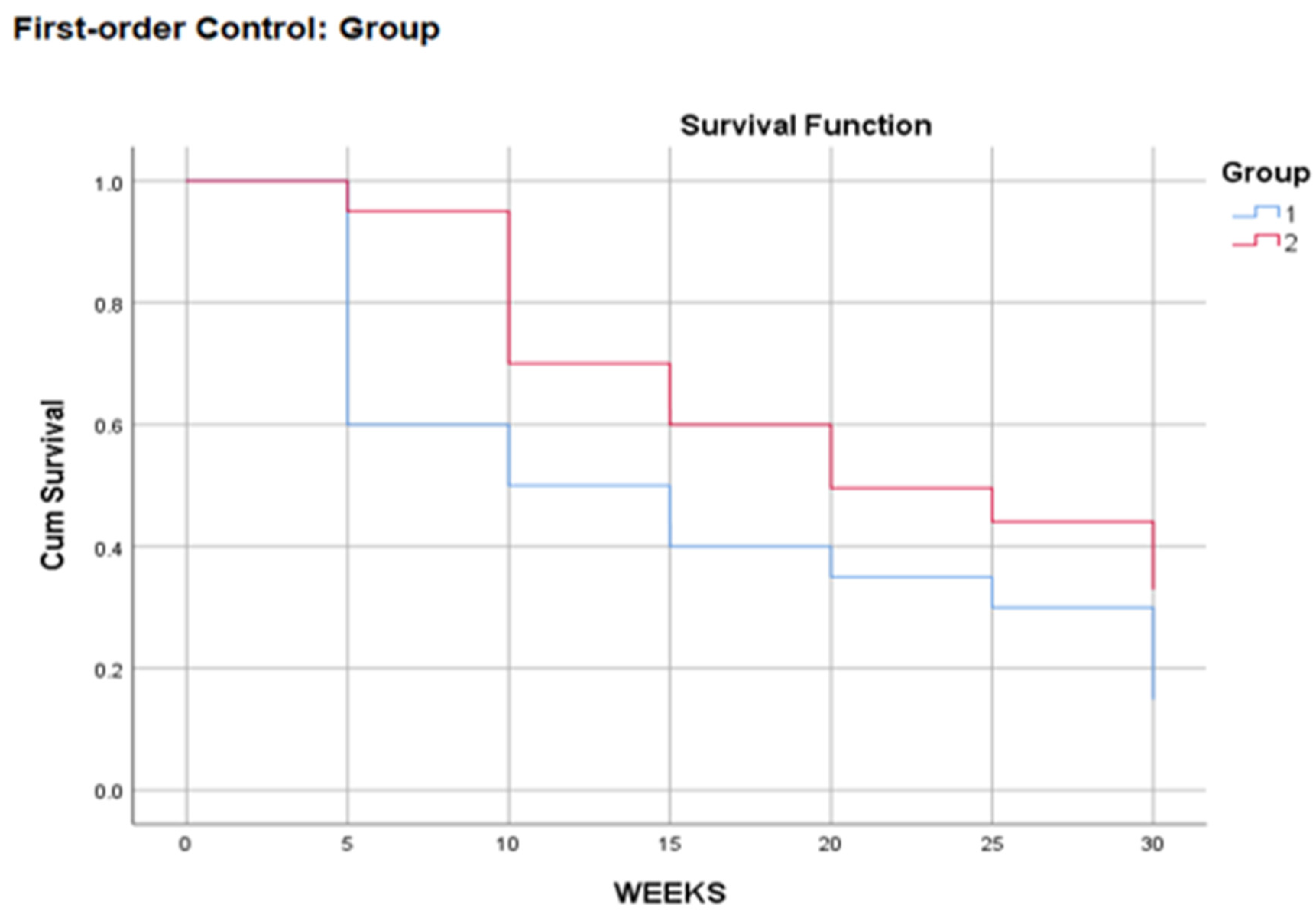
Figure 2.
Hazard Function.
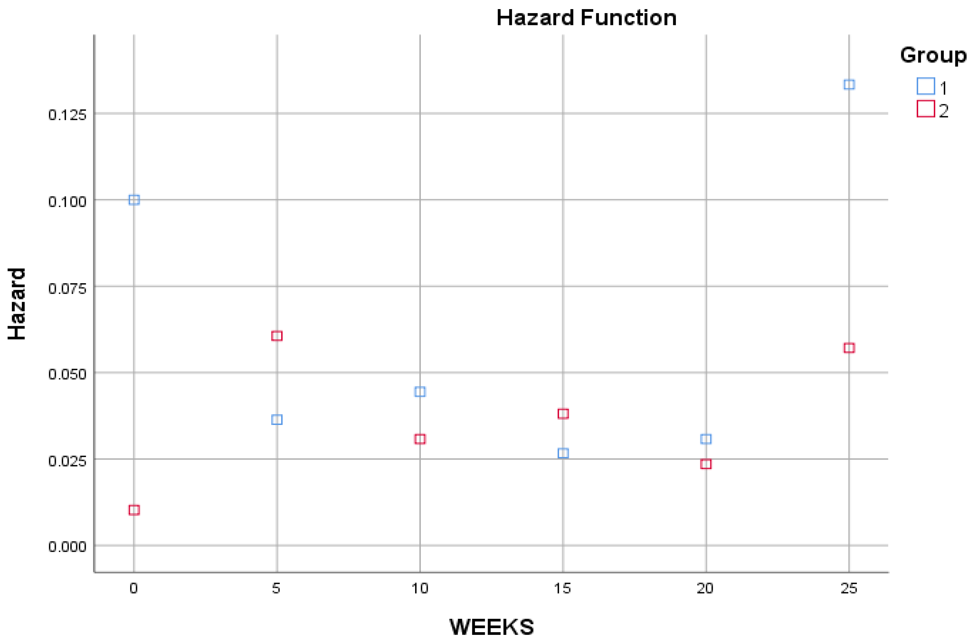
Figure 3.
Survival Functions.
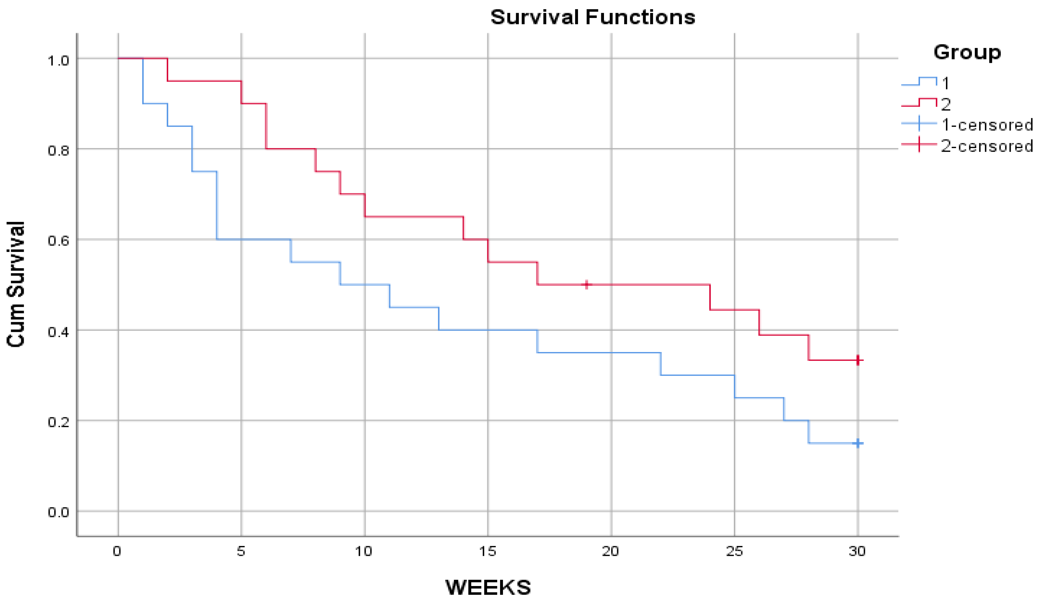
Figure 4.
Hazard Function.
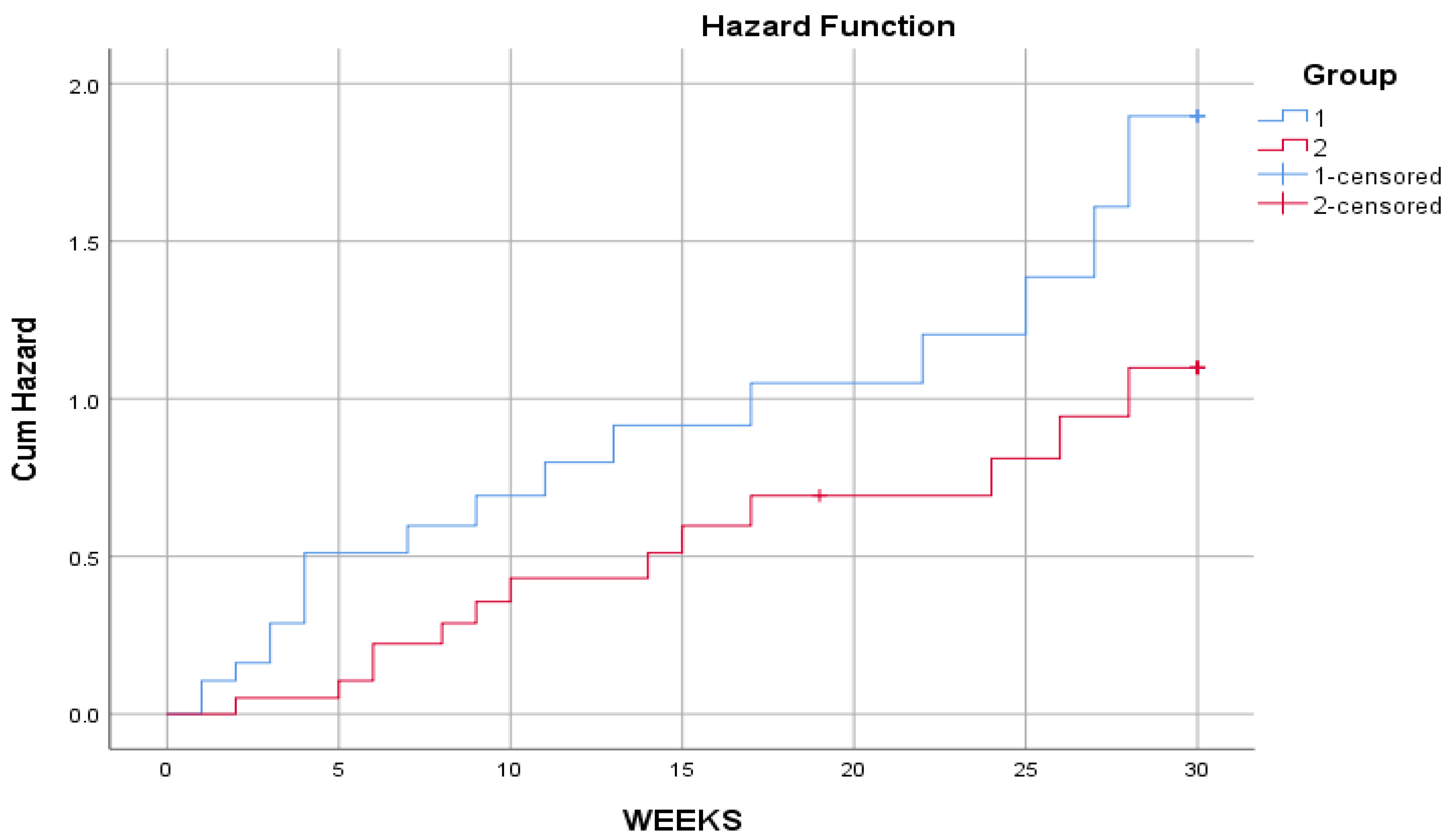

Table 1.
Life table for a period.
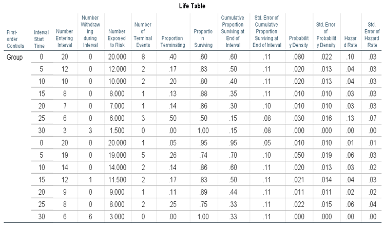 |
Table 2.
Median Survival Time.
| First-Order Controls | Med Time | |
| Group | 1 | 10.00 |
| 2 | 19.79 | |
Table 3.
Comparisons for Control Variable: Group.
| Overall Comparisons | ||
| Wilcoxon (Gehan) Statistic | df | Sig. |
| 3.122 | 1 | 0.077 |
| a. Comparisons are exact | ||
Table 4.
Case Processing Summary.
| Censored | ||||
| Group | Total N | N of Events | N | Percent |
| 1 | 20 | 17 | 3 | 15.0% |
| 2 | 20 | 13 | 7 | 35.0% |
| Overall | 40 | 30 | 10 | 25.0% |
Table 5.
Survival Table.
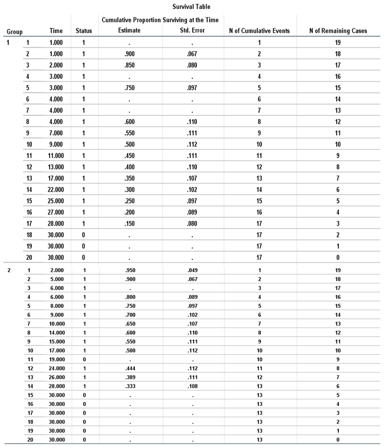 |
Table 6.
Means and Median for Survival Time.
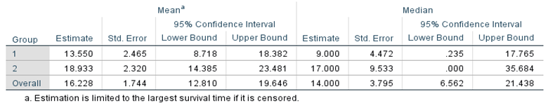 |
Table 7.
Overall Comparisons.
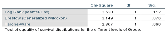 |
Table 8.
Brain Tumor Patients Data.
| ID | Time (weeks) | Event (Death=1, Survival=0) | Group (1: Conventional, 2: New Treatment) |
|---|---|---|---|
| 1 | 1 | 1 | 1 |
| 2 | 1 | 1 | 1 |
| 3 | 2 | 1 | 1 |
| 4 | 3 | 1 | 1 |
| ... | ... | ... | ... |
Disclaimer/Publisher’s Note: The statements, opinions and data contained in all publications are solely those of the individual author(s) and contributor(s) and not of MDPI and/or the editor(s). MDPI and/or the editor(s) disclaim responsibility for any injury to people or property resulting from any ideas, methods, instructions or products referred to in the content. |
© 2025 by the authors. Licensee MDPI, Basel, Switzerland. This article is an open access article distributed under the terms and conditions of the Creative Commons Attribution (CC BY) license (https://creativecommons.org/licenses/by/4.0/).
Copyright: This open access article is published under a Creative Commons CC BY 4.0 license, which permit the free download, distribution, and reuse, provided that the author and preprint are cited in any reuse.


