
Submitted:
22 July 2025
Posted:
23 July 2025
You are already at the latest version
Abstract
With the development of the Industrial Internet of Things (IIoT) technology, fault diagnosis has emerged as a critical component of its operational reliability, and machine learning algorithms play a crucial role in fault diagnosis. To achieve better fault diagnosis results, it is necessary to have a sufficient number of fault samples participating in the training of the model. In actual industrial scenarios, it is often difficult to obtain fault samples, and there may even be situations where no fault samples exist. For scenarios without fault samples, accurately identifying the unknown faults of equipment is an issue that requires focused attention. This paper presents a method for the normal-sample-based mechanical equipment unknown fault detection. By leveraging the characteristics of the auto-encoder network (AE) in deep learning for feature extraction and sample reconstruction, normal samples are used to train the AE network. Whether the input sample is abnormal is determined via the reconstruction error and a threshold value, achieving the goal of anomaly detection without relying on fault samples. In terms of input data, the frequency domain features of normal samples are used to train the AE network, which improves the training stability of the AE network model, reduces the network parameters, and saves the occupied memory space at the same time. Moreover, this paper further improves the network based on the traditional AE network by incorporating a convolutional neural network (CNN) and a long short-term memory network (LSTM). This enhances the ability of the AE network to extract the spatial and temporal features of the input data, further improving the network’s ability to extract and recognize abnormal features. In the simulation part, through public datasets collected in factories, the advantages and practicality of this method compared with other algorithms in the detection of unknown faults are fully verified.
Keywords:
industrial internet of things
; fault diagnosis
; auto-encoder network
; convolutional neural network
; long short-term memory network
1. Introduction
With the rapid technological evolutions in manufacturing, we are now experiencing a new generation of industrial revolution, that is IIoT [1,2,3,4,5]. In critical sectors covered by the Industrial Internet, such as manufacturing, energy, transportation, and healthcare, equipment failures can lead to production line disruptions, inefficient resource utilization, safety risks, and ecological and environmental hazards [6,7,8]. Typical scenarios include: downtime of key processing equipment in discrete manufacturing workshops, which can incur direct production losses ranging from hundreds to tens of thousands of dollars per hour for a single machine; failures in energy transmission and distribution systems, which may cause regional power outages affecting tens of thousands of users; and malfunctions of core components in rail transit, which could jeopardize operational safety. Therefore, establishing a precise equipment fault diagnosis system to achieve early defect identification and potential fault prediction has become a core technical requirement for safeguarding industrial systems’ reliability, safety, and economic efficiency.
With the development of industrial big data and machine learning technologies [9], data-driven fault classification algorithms have made remarkable progress. However, their core relies on an adequate number of labeled fault samples to build training models [10]. Nevertheless, in real industrial scenarios, equipment failures are significantly random and sporadic, and it is difficult to define fault types in advance [11]. Moreover, for large and critical equipment, failures may lead to catastrophic consequences. The operation and maintenance strategies rely on high-frequency manual inspections and component replacements, resulting in an extreme shortage of real fault data [12]. Against this backdrop, breaking through the strong dependence of traditional supervised learning on labeled samples and developing unknown fault detection methods suitable for few-sample or no-sample scenarios has become a key research direction in the field of industrial Internet fault diagnosis [13]. Traditional methods relying on regular maintenance and manual inspections are inefficient. It is difficult to monitor the equipment degradation trend in real time, and it is even more difficult to effectively predict sudden failures [14]. There is an urgent need to achieve a paradigm shift from "post-failure repair" to "predictive maintenance" through intelligent diagnosis technologies[15]. In the field of industrial Internet equipment fault diagnosis, deep learning technologies, by constructing multi-layer nonlinear mapping networks, have provided a revolutionary solution for unknown fault detection. As a typical unsupervised learning paradigm, the Autoencoder (AE) minimizes the mean squared error between the input and the reconstructed output, realizing feature compression and reconstruction of high-dimensional signals in the hidden layer[16]. Its core advantage lies in that it only requires normal samples to build a fault detection model. When an abnormal sample is input, the difference in feature distribution that has not participated in the training will lead to significant reconstruction errors. By setting an adaptive threshold, unknown faults can be accurately identified [17]. Traditional AEs and their variants (such as sparse autoencoders and deep convolutional autoencoders) perform excellently in static data processing. However, when facing dynamic signals such as time-series vibrations and currents collected by industrial sensors, due to the lack of the ability to model the correlation of time series and spatial local features, the accuracy of abnormal identification is limited [18]. In response to this challenge, an improved AE architecture that integrates a CNN Network and an LSTM Network is needed. By extracting the frequency-domain spatial features and time-series dynamic patterns of signals, it significantly enhances the fault representation ability under complex working conditions [19]. In the scenarios of industrial predictive maintenance, the deep learning-driven fault detection system shows unique advantages: by continuously collecting equipment operation data, the model can monitor the changes in reconstruction errors in real time and identify the performance degradation trend at the initial stage of device aging. When an abnormality is detected and maintenance is completed, the newly obtained fault data can be used for model iteration, forming a data closed loop of "detection - maintenance - optimization"[20]. This capability enables the system not only to detect unknown faults but also to accurately predict the types of faults through continuous learning of historical fault patterns, guide the formulation of targeted maintenance strategies, greatly improve the operation and maintenance efficiency and reliability of industrial equipment, and promote the paradigm shift of smart factories from passive maintenance to active health management[21].
Amid substantial research on fault detection, deep learning methods arise as a pivotal direction. The main reason lies in deep learning methods’ capability to automatically extract data features through continuous learning. Their superior adaptability and generalization capabilities enable effective handling of complex nonlinear data, a trait that has attracted significant research interest from academia and industry. [22]. An intelligent diagnostic method utilizing Deep Neural Networks (DNNs) was proposed in [23] to address the shortcomings of traditional methods in handling complex nonlinear data. With the prominence of CNN capability in local feature extraction, the authors in the paper [24] proposed a CNN-based prediction model, which achieved the classification of mechanical equipment faults and attained high accuracy even with limited data sources. To further improve the performance of algorithms in equipment fault diagnosis, researchers have begun to combine neural network algorithms with traditional machine learning algorithms. In [25], the researchers integrated CNN with SVM to propose a CNN-SVM bearing fault diagnosis scheme, which uses CNN to extract data features and then employs SVM for classification. This approach reduces system runtime while improving classification accuracy. In reference [26], the authors developed a novel RF-based CNN model, incorporating a dropout layer into the CNN to prevent overfitting. Experimental results confirmed that this method outperforms traditional algorithms such as SVM, CNN, and RF. As input time-series data lengthen, Long Short-Term Memory (LSTM) networks have been adopted in fault diagnosis to capture long-range temporal dependencies. Reference [27] presented a fault diagnosis method for wind turbine gearboxes leveraging an LSTM-based approach. It optimizes the network with cosine loss to reduce the impact of signal intensity on diagnostic accuracy and enhance diagnostic precision. The synergistic integration of CNN and LSTM facilitates concurrent extraction of localized spatial features and long-term temporal dependencies from data. Reference [28] designed a novel CNN-LSTM neural network that takes raw data collected by sensors as input to achieve end-to-end fault detection. Meanwhile, Reference [29] proposed a deep neural network based on a bidirectional convolutional LSTM network to address the complex responses of planetary gearboxes, determining the type of planetary gearbox faults by automatically extracting the spatiotemporal features of input signals. Reference [30] proposed a new convolutional LSTM network to fully utilize signal features and improve detection accuracy, using raw signals combined with Fourier-transformed and wavelet-transformed signals as inputs to process and classify this multichannel information. This method maintained high accuracy even with shorter input signal segments. The papers [31,32,33,34,35,36,37] have made contributions to the anomaly detection of equipment from different perspectives. The development of autoencoder (AE) networks in the field of deep learning has provided new insights for anomaly detection in mechanical equipment. AE is an unsupervised neural network model with a symmetric network structure [38]. Researchers use the symmetric structure of AE to restore original samples from features extracted by the encoder through the decoder. When only normal samples are trained, the reconstruction error between the input samples and the generated samples continuously decreases with the increase in training iterations. However, when an abnormal sample is input, since it did not participate in training, the network cannot reconstruct it well, resulting in a large reconstruction error. By setting a reasonable reconstruction error threshold, abnormal samples can be accurately detected [39]. The papers [40,41,42,43,44,45] demonstrate the application scenarios of AE networks, which achieve the function of anomaly detection but cannot classify abnormal samples.
In summary, autoencoders (AEs) trained exclusively on normal samples can only classify normal samples, but inherently lack the capability to distinguish abnormal samples. If classification algorithms are applied to fault detection, they can only assign samples to predefined known classes. When unknown faults emerge, they may lead to erroneous judgments by maintenance personnel, reduce maintenance efficiency, and cause certain production losses. Therefore, the detection of unknown fault types amid known faults is a challenge that demands attention. This paper presents the following primary contributions to fault detection in IIoT:
- This paper proposes a DC-LSTM-AE model based on deep CNN and LSTM. The model extracts spatial features via a five-layer CNN and captures the long-term dependencies of time-series data through LSTM, enabling spatiotemporal feature fusion for high-dimensional nonlinear time-series signals in industrial environments. This approach addresses traditional autoencoders’ limitations in extracting features from complex signals and enhances unknown fault detection performance.
- To address the core problem of scarce fault samples in industrial scenarios, we design a training procedure using only normal samples. By leveraging the reconstruction error characteristics of autoencoders, a benchmark feature space is constructed through training with normal samples. When abnormal samples are input, their absence from the training process leads to significantly increased reconstruction errors. Anomaly detection is achieved by setting thresholds based on the Pauta criterion. This strategy breaks through the dependence of traditional supervised learning on fault samples, providing a feasible solution for early equipment maintenance.
- In this study, we employ sliding windows and fast Fourier transform (FFT) to convert time-series signals into spectral features. This reduces data dimensions while preserving key information, enhances model training stability, and lowers memory consumption. The L2 regularization term is introduced to optimize the loss function, suppress overfitting, and enhance the model’s generalization ability. By dynamically adjusting the regularization coefficient through cross-validation, a balance is achieved between model complexity and detection accuracy, making it suitable for real-time detection requirements in industrial sites.
- We evaluate our method using two industrial datasets: the Southeast University gearbox dataset (containing four fault types) and a constant-speed water pump dataset from factory settings (with one fault type). Compared to traditional autoencoders, deep convolutional autoencoders, and some machine learning algorithms, the results show that DC-LSTM-AE significantly outperforms the comparative methods in metrics such as accuracy and precision. Especially when processing unknown faults with high feature similarity, it exhibits more pronounced reconstruction error distinctions. These results conclusively validate the method’s effectiveness and industrial applicability.
These contributions collectively advance the understanding and development of fault detection problems in IIoT, providing a robust foundation for future work and practical applications. The remainder of this article is organized as follows: Section II provides the system models and an overview of the fault detection model in the IIoT situation. The fault detection strategy based on the DC-LSTM-AE algorithm is created in Section III. The simulation results and performance analysis are discussed in Section IV. In Section V, the conclusions are given.
2. System Model
The model proposed in this paper is shown in Figure 1. An improved DC-LSTM-AE model based on deep CNN and LSTM is developed by enhancing the traditional auto-encoding algorithm. Specifically, the CNN component processes high-dimensional and complex-structured sensor signals, significantly improving the model’s representation capability for input data. The LSTM algorithm model can better capture long-term dependency relationships, thereby improving fault detection accuracy. The combination of CNN and LSTM further enhances the model’s ability to extract and analyze the spatial and temporal information of sensor data. Consequently, the neural network has strong noise immunity and enhanced stability in industrial environments.
The DC-LSTM-AE algorithm model architecture includes an encoder and a decoder. The encoder employs a five-layer CNN for spatial feature extraction, and each layer of the CNN contains a normalization layer, an activation layer, and a pooling layer. This study substitutes LeakyReLU for the traditional ReLU function in activation layers to mitigate the representational capacity degradation caused by neuronal deactivation, which occurs when ReLU outputs zero for negative inputs. LeakyReLU addresses this issue by introducing a small non-zero gradient (typically 0.01 or 0.02) in the negative domain. Its mathematical formulations are as follows:
where is a small constant. This ensures that when the input is negative, the neuron avoids complete deactivation by retaining a small gradient, thereby alleviating vanishing gradients and preserving the network’s learning capacity. The pooling layer is applied to retain certain prominent features maximally, thereby enhancing the model’s fault detection accuracy. Following convolution, an LSTM network is applied to extract temporal features. Subsequently, a fully connected layer (FCL) is used for feature integration and dimensionality reduction.
In the decoder, the encoder’s output features are first expanded via an FCL network. Then, the temporal features are restored using an LSTM network. Furthermore, the spatial features of the samples are recovered via a five-layer transposed CNN to ultimately achieve sample reconstruction. Each layer of the transposed CNN also includes a normalization layer, an activation layer, and an unpooling layer. Here, the LeakyReLU activation function is also used in the activation layer.
3. The Proposed DC-LSTM-AE Algorithms
The working environment of actual industrial production is extremely complex, with complicated and changeable working conditions, and most of the signals collected by sensors are non-stationary and non-linear data[46]. Under these conditions, fault detection and diagnosis require more powerful feature extraction tools to obtain more valuable information from such signals. Deep learning addresses this through powerful feature extraction and learning capabilities enabled by deep neural networks with increased parameters and depth[47].
3.1. The CNN Algorithm
CNN is a deep learning model widely applied in time-series signal analysis. They excel at processing grid-structured data and are extensively used in mechanical equipment fault detection, demonstrating excellent performance in signal processing and feature extraction [48]. The core idea of CNN is to extract local features via convolution operations and reduce computational complexity via pooling. Key CNN principles are local connectivity, parameter sharing, and pooling operations, allowing identification of discriminative patterns across signal locations. Local connectivity in CNN ensures that each neuron connects only to a localized region of the input, rather than the entire input layer as in fully connected layers. In mechanical fault signals, local features are critical diagnostic information, and local connectivity enables the targeted extraction of information from these regions, enhancing the detection accuracy. Parameter sharing refers to the use of the same convolution kernel for the connections between all output layer nodes and their corresponding local regions in the input layer. This approach significantly reduces trainable parameter counts, particularly for high-dimensional data, enabling efficient CNN training and deployment in resource-constrained environments. CNN is a hierarchical model whose basic structure consists of an input layer, convolutional layers, pooling layers, fully connected layers, and an output layer with detailed layer specifications provided below [49]:
Input Layer: The input layer serves to receive raw data as input and transmit this information to subsequent layers for feature extraction. In the context of mechanical equipment fault detection, the input data can be time-series data collected by sensors or preprocessed spectrograms.
Convolutional Layers: The convolutional layer extracts local features from the input data, which are leveraged by CNN in mechanical equipment fault diagnosis to identify potential anomalies and faults. The convolutional layer scans the input data using multiple convolution kernels to extract local features in different dimensions. The core formula for the convolution operation is as follows:
Where x is the input signal, y is the output signal, w is the convolution kernel, b is the bias term, and M and N are parameters representing the size of the convolution kernel.
Pooling Layers: The pooling layer is an important component of CNN, mainly used for dimensionality reduction of feature maps, significantly reducing model parameters while preserving critical information. The operation improves the computational efficiency and enhances its robustness and translation invariance to data. In the fault detection of mechanical equipment, the pooling layer facilitates extracting key features from vibration signals or spectrograms while reducing the impact of noise.
Fully Connected Layers: The fully connected layer is typically located at the back end of the network. Its main function is to utilize the features extracted by the preceding convolutional and pooling layers for classification, regression, or other tasks. In mechanical equipment fault detection, the fully connected layer transforms analyzed feature representations into diagnostic labels of health states, performing critical fault classification decisions.
3.2. The LSTM Algorithm
The LSTM network introduces memory cells, input gates, output gates, and forget gates, which are based on the recurrent neural network (RNN), which enables it to effectively handle long-sequence problems [50,51]. The structure diagram of the network is shown in Figure 2.
Input Gate: The input gate computes an affine transformation of the current input and the hidden state output at the previous moment, transforming it via sigmoid activation to the range of [0,1] to generate a gating signal. Its function is to determine which information is selected for storage in the cell state at the current time step. The specific calculation formula is as follows:
Where and are the weight parameters of the input gate and is the bias parameter of the input gate. In mechanical equipment fault detection, the input gate mechanism prevents critical time series information from being discarded, reduces sensitivity to transient irrelevant signals, and consequently extracts key features from long-term data trends.
Forget Gate: The Forget Gate determines which portions of the prior cell state to preserve and which to discard at the current time step through gated operations. This mechanism ensures that the model can dynamically adjust the content of the memory units to adapt to changes in the input data. The calculation formula for the gating signal is as follows:
Where and are the weight parameters of the forget gate and is the bias parameter of the forget gate. In fault detection, the forget gate retains the maximum amount of information relevant to fault patterns. Conversely, for random noise or irrelevant operational signals, it filters out such information, effectively suppressing their interference with the judgment of the equipment’s state.
Memory Cell: The Memory Cell is the core component of the LSTM network, responsible for storing and maintaining long-term information and dynamically updating information flow through a gating mechanism. Its operations involve two key components: information retained from the previous time step and information input at the current time step. The specific formulas are as follows:
Where denotes the input information and is the state information of the memory cell at the current time step. In equipment fault detection, signals collected by sensors may contain a large amount of noise and redundant features. This approach can adaptively filter important information, effectively mitigating key information loss in long time series.
Output Gate: The output gate primarily controls information flow to the next time step. It dynamically selects which historical information to extract from the memory cells for output to the current hidden state. The relevant formula is as follows:
Where and are the weight parameters of the output gate, is the bias parameter of the output gate, and is the gating signal of the output gate with a value range of [0, 1]. In mechanical equipment fault detection, the output gate extracts and outputs content related to fault features from the memory cells. This enables real-time monitoring of operational status and prediction of future failure risks.
3.3. The AE Algorithm
AE is a common unsupervised learning method, which mainly consists of two parts: an encoder and a decoder, and has a symmetrical structure [52]. Autoencoders are typically used for dimensionality reduction of high-dimensional data. When high-dimensional data is input into an AE network, it produces output data matching the input dimension. The network is continuously trained by minimizing the reconstruction error between the output data and the input data. Finally, the middle hidden layer yields a low-dimensional representation, achieving dimensionality reduction and feature extraction. It aims to learn a low-dimensional data representation by minimizing reconstruction error. During fault detection, the deviation in reconstruction error of test data from normal data serves to detect anomalies [53].
The structure of the AE is shown in Figure 3. For high-dimensional input data , where n represents the number of data points, the corresponding low-dimensional representation is obtained through the encoder. The low-dimensional representation of the data is then input into the decoder to obtain the corresponding output data. Assuming the input data is , the formulas for the encoding and decoding processes can be expressed as:
Where is the low-dimensional feature vector obtained by the encoder; and represent the activation functions of the encoder and decoder, respectively; and are the weights and biases of the encoder; and are the weights and biases of the decoder; and denotes the output data obtained by the decoder.
During the training process, the loss function of AE generally selects the MSE loss function:
The above function iteratively updates the network parameters via backpropagation and gradient descent algorithms, minimizing the reconstruction error between the output data and the input data, and the middle hidden layer of the network obtains a low-dimensional representation of the input data. When the AE network is trained, new input data that significantly differs from the training data will be poorly reconstructed by the network, resulting in a large reconstruction error. Comparing the magnitudes of reconstruction errors across individual samples enables the identification of anomalous samples.
3.4. The DC-LSTM-AE Algorithm
The specific process of the mechanical equipment’s unknown fault detection method based on normal samples proposed is shown in Figure 4:
From the flow chart, vibration signals from mechanical equipment are first processed to observe variations. The sliding window method segments normal samples into frames. Based on FFT requirements, model input size constraints, and the trade-off between data overlap and information novelty per sample, the window width and step size are set to 2048 and 1024, respectively. This windowing process yields time-series normal samples. Convert the obtained time-series normal signal into the frequency domain via FFT to generate the training dataset , where n denote the number of normal samples. This can be expressed by the formula:
where represents the m-th frequency value of the i-th sample, denotes the k-th time-series value of the i-th sample, and l is the size of the sliding window. Due to the symmetry of the Fourier transform, we retain only half of the spectrum after the Fourier transform to reduce the number of network parameters. The training dataset is subjected to Z-Score standardization processing [54] to obtain the standardized dataset . The specific formula is:
where is the standardized value of the j-th feature in the i-th sample. is the j-th feature value of the i-th sample. represents the set of all values for the j-th feature across all training samples. denotes the mean value of the j-th feature computed from the training samples. denotes the standard deviation of the j-th feature computed from the training samples. After standardizing the training dataset, store the computed mean and standard deviation values for future use.
Subsequently, the standardized dataset of normal samples is used to train the designed DC-LSTM-AE model. After training, both the model parameters and the reconstruction error threshold derived from normal samples are stored. This threshold is then used to classify test samples as normal or abnormal. Once the trained model and the reconstruction error threshold are obtained, mechanical equipment anomaly detection proceeds as follows. Newly acquired sensor time-series signals are first converted to the frequency domain via the FFT. These frequency-domain signals are then standardized by applying the mean and standard deviation saved during the Z-score normalization of the training data. The preprocessed samples are subsequently input into the saved DC-LSTM-AE model to generate their reconstructions. The reconstruction error between each input and its reconstructed counterpart is calculated and compared against the saved threshold. If the error is less than or equal to the threshold, the sample is classified as normal. Conversely, if the error exceeds the threshold, the sample is classified as abnormal, triggering an alarm to alert staff. This prompts necessary corrective actions to prevent further damage, avoid production losses, and mitigate safety risks.
4. Results Simulation and Discussion
To fully validate the practicality and effectiveness of the proposed normal-sample-based fault detection method for mechanical equipment, multiple datasets were selected for experimental verification, including the gearbox dataset from Southeast University and the constant-speed water pump dataset collected in actual factories. Furthermore, the proposed method was extensively compared with established anomaly detection techniques and various autoencoder network architectures. These comparisons aimed to demonstrate the method’s superiority in detecting unknown faults.
4.1. Experimental Setup
Without loss of generality, the simulation parameters were set as follows in Python for WIN10. The Computer Configuration was as follows: the Processor (CPU) was an Intel(R) Core(TM) i7-10750H CPU @ 2.60 GHz; the Clock Speed was 2.59 GHz; the Memory (RAM) was 1024 GB with an NVIDIA GeForce GTX 1650 Ti. After the data collected from the sensor undergoes sliding window sampling and FFT processing, each sample has a dimensionality of 1024. Table 1 details the DC-LSTM-AE network architecture and layer output dimensions, designed according to this input size. For model training, we use the Adam optimizer with a learning rate of 0.001, training for 500 epochs with a batch size of 128.
4.2. Experimental Datasets
4.2.1. The Gearbox Dataset from Southeast University
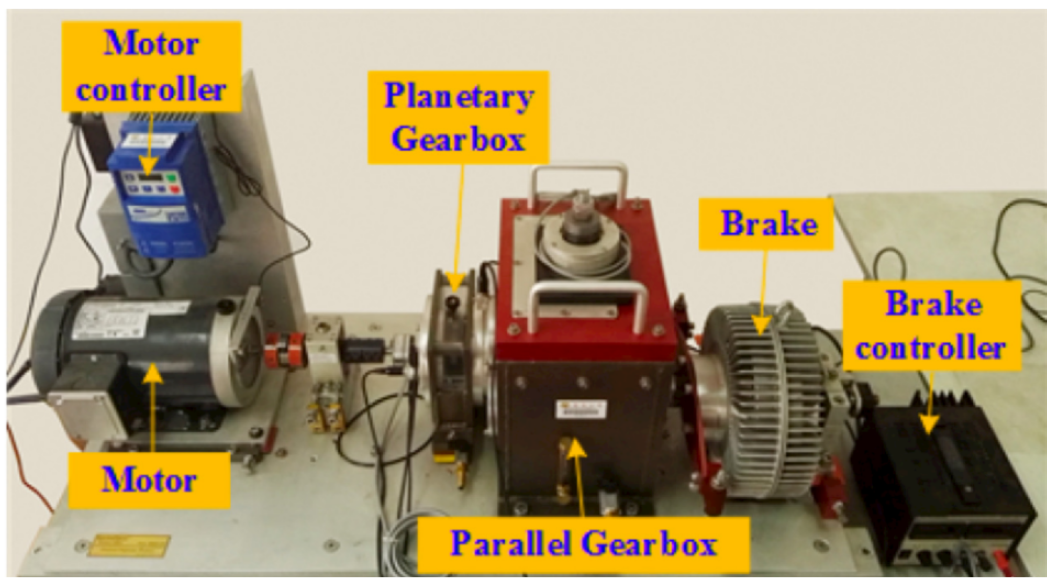
The gearbox dataset from Southeast University was collected by a gearbox test rig, as shown in Figure 1. The test rig consists of a motor, motor controller, planetary gearbox, reduction gearbox, brake, and brake controller. In this experiment, the gearbox status data were collected under the working conditions of a rotational speed of 20 Hz and a load of 0 V, including healthy data under normal operation and four types of fault data. The fault types are: crack in gear, tooth breakage, root crack of gear, and surface wear of gear. The dataset contains signals collected by multiple sensors. To better analyze the operating status of the gearbox, the vibration signals in the x-direction of the planetary gearbox were selected as the signal source in this experiment.
Figure 5.
Gearbox Test Rig of Southeast University Dataset
To demonstrate the proposed algorithm’s ability in mechanical equipment fault detection without relying on fault samples, the normal samples were first randomly divided into training and test sets at an 8:2 ratio. Subsequently, 200 samples were randomly selected from each type of fault sample as test samples for unknown faults. The model was trained exclusively on normal samples, while testing utilized both normal samples and samples from four fault types. The detailed division of the number of training and test samples in the dataset is shown in Table 2.
4.2.2. Constant-Speed Water Pump Dataset
To validate the practicality of the model proposed in this chapter, a constant-speed water pump dataset collected from an actual factory was selected for experimental verification. Beyond normal pump operation measurements, this dataset also comprises bearing fault condition data. Similarly, only normal samples were used for training, while both normal and fault samples were used for testing. The ratio of normal samples used for training to those used for testing was 8:2. The specific division of the number of training and test samples is shown in Table 3.
4.3. Evaluation Metrics
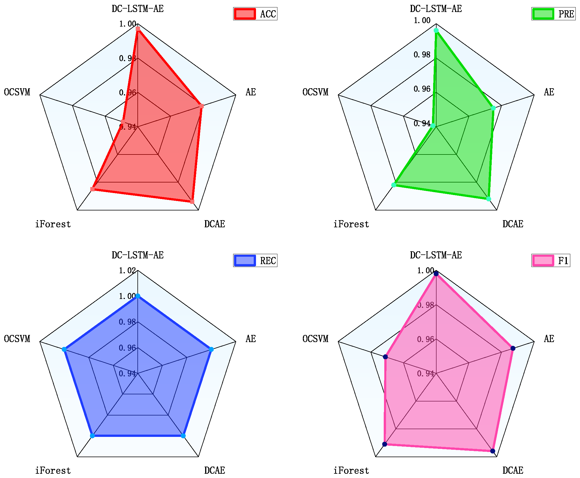
Due to a significant imbalance between fault and normal data proportions, mechanical equipment anomaly detection faces substantial class imbalance challenges. When the number of samples in one category of the data is significantly smaller than that in other categories, simply using accuracy to compare the performance between algorithms often leads to an unfair evaluation. Therefore, to more effectively evaluate the detection performance of the model for unknown fault samples, this paper uses accuracy (ACC), precision (PRE), recall (REC), and F1-score (F1) as evaluation indicators. The closer the values of these indicators are to 1, the better the detection effect. The specific calculation formulas for each indicator are as follows:
Herein, denotes the number of actual fault samples correctly predicted as faulty, represents the number of actual normal samples correctly predicted as normal, signifies the number of actual fault samples incorrectly predicted as normal, and indicates the number of actual normal samples incorrectly predicted as faulty. The -score, defined as the harmonic mean of precision () and recall (), provides a comprehensive evaluation of fault detection performance by integrating these complementary metrics.
4.4. Experimental Results and Analysis
To evaluate the abnormal sample detection performance of the proposed model, we benchmarked it against two common anomaly detection algorithms: Isolation Forest (iForest) and One-Class Support Vector Machine (OCSVM). In the iForest algorithm, the number of isolation trees was set to 100, the maximum depth of each tree was 8, and each tree randomly selected 256 samples for training. For the OCSVM algorithm, the Gaussian kernel function served as the kernel, and the proportion of abnormal samples was set to 0.02. Furthermore, to evaluate the superiority of the designed DC-LSTM-AE model in feature extraction compared to traditional autoencoder networks, comparisons were also conducted with the traditional autoencoder (AE) and the deep convolutional autoencoder (DCAE) [42,55]. The network depth of both AE and DCAE was the same as that of the DC-LSTM-AE model. In the AE model, all hidden layers were composed of fully connected layers, while in the DCAE network, the hidden layers consisted of convolutional layers and fully connected layers. During the experiment, each algorithm was trained using only normal samples and tested using both normal and fault samples, with the ratio of normal samples for training to testing set at 8:2.
4.4.1. Experimental Verification of Southeast University Gearbox Dataset
To validate the effectiveness of the proposed normal-sample-based mechanical fault detection method, we first conducted experiments using the Southeast University (SEU) gearbox dataset. Given the scarcity of fault samples in industrial settings, our method’s practicality is demonstrated by training exclusively on normal samples while evaluating performance using both normal and fault samples. Figure 6 presents the DC-LSTM-AE model’s reconstruction errors for test data. The results demonstrate lower reconstruction errors for normal samples compared to fault samples. Moreover, the reconstruction errors of normal test samples generally remain below the threshold, whereas those of unknown fault samples mostly exceed it. The unknown fault detection successfully identifies all four fault types while maintaining high classification accuracy for normal samples. Furthermore, distinct characteristics of the four fault types result in varying degrees of deviation from the normal sample. Since the model is only trained on normal samples, the differences in reconstruction errors between different types of faults are relatively large, but show little variation within the same fault type, because samples of the same fault share similar characteristics. This is also reflected in Figure 6.
The proposed DC-LSTM-AE framework integrates a 5-layer CNN and LSTM modules into the encoder of a traditional autoencoder. By combining CNN-based spatial feature extraction with LSTM-based temporal modeling, the model effectively learns spatiotemporal representations, thereby enhancing its capability to detect previously unseen faults. To demonstrate the detection advantages of the proposed DC-LSTM-AE model for unknown fault samples, the AE model and the DCAE model were selected for comparative analysis. Figure 7 shows the reconstruction errors of the test data of the AE model and the DCAE model in the gearbox dataset. It can be seen from the figure that the AE model’s limited feature extraction capability leads to misidentification of most unknown fault samples as normal when their features resemble those of normal samples, despite the correct detection of some normal samples and specific fault types. For the DCAE model, the incorporation of CNN significantly enhances feature extraction capability, enabling the correct detection of unknown faults. However, compared with the DC-LSTM-AE model, it lacks temporal information extraction, resulting in a small gap between the reconstruction errors of the model for unknown fault samples and those of normal samples. When the fault features are relatively similar to those of normal samples, there is still a risk of detection errors. However, for the DC-LSTM-AE model, due to the large difference in reconstruction errors between normal samples and fault samples, it exhibits superior detection capability for unknown faults and precisely identifies even small equipment faults.
To demonstrate the advantages of the proposed DC-LSTM-AE model for mechanical equipment unknown fault detection, the iForest model and the OCSVM model were selected for comparative analysis. The T-SNE algorithm was used to visualize the high-dimensional features of the test samples[56], and Figure 8 shows the detection results of different algorithms for the test samples of the gearbox dataset. The first image shows the distribution of normal and fault samples in the real test samples. The detection results of the DC-LSTM-AE model show that all unknown fault samples are correctly detected, and only a few normal samples are mistakenly detected as unknown fault samples. However, although the traditional iForest algorithm accurately detects most normal samples, most unknown fault samples are mistakenly detected as normal samples. The OCSVM algorithm correctly detects all unknown fault samples, but most normal samples are detected as fault samples, which will lead to many false alarms in practical applications. For the gearbox dataset, the detailed experimental results of each algorithm are shown in Figure 9. It can be seen from the table that the proposed DC-LSTM-AE-based method for mechanical equipment unknown fault detection outperforms all comparable algorithms across all evaluation metrics when trained exclusively on normal samples.
4.4.2. Experimental Validation of Constant-Speed Water Pump Dataset
To further validate the effectiveness of the normal-sample-based mechanical equipment unknown fault detection in practical industrial environments, experimental validation was conducted on a constant-speed water pump dataset collected from actual factories. For this dataset, only normal samples were used for model training, and both normal and unknown fault samples were used for testing, with the training-to-testing ratio of normal samples set at 8:2. Figure 10 shows the reconstruction errors of the test data from the DC-LSTM-AE model for the constant-speed water pump dataset. It can be seen that a significant difference in reconstruction errors between normal samples and unknown fault samples.
According to the judgment criteria for unknown fault detection, only 1 normal sample was misclassified as a faulty sample in the test data, and all unknown fault samples were correctly detected, indicating that the proposed method also demonstrates excellent detection performance for unknown faults in practical industrial environments. Furthermore, observing the reconstruction errors of unknown fault samples reveals that the reconstruction error of faulty samples gradually increases over time, suggesting that the degree of equipment damage intensifies in practical industrial settings. Owing to its high sensitivity to unknown faults, it can detect anomalies during the initial phase of fault inception. Therefore, issuing early warnings and implementing effective maintenance at the early fault stage can effectively prevent further equipment damage, improve production efficiency, safeguard the lives and property of frontline workers, and avoid serious production accidents.
To highlight the superiority of the DC-LSTM-AE model over traditional autoencoder structures in detecting unknown faults, the AE and DCAE models were also tested on the constant-speed water pump dataset. Figure 11 shows the reconstruction errors of the AE and DCAE models on the test data from this dataset.
It can be observed that a significant gap between the reconstruction errors of normal samples and those of unknown fault samples, attributable to pronounced feature dissimilarity. Moreover, the AE model’s limited feature extraction capability results in ineffective reconstruction of normal samples, leading some normal samples to be misclassified as faulty. In contrast, the DC-LSTM-AE model effectively captures both spatial and temporal information of samples via its CNN and LSTM networks. Compared to the AE and DCAE models, the DC-LSTM-AE model achieves greater separation between normal and unknown fault reconstruction errors while maintaining more stable error distributions. These results validate the superiority of the DC-LSTM-AE model over traditional autoencoder structures in detecting unknown faults.
To demonstrate the advantages of the normal-sample-based mechanical equipment unknown fault detection over traditional machine learning algorithms in practical industrial environments, experiments were conducted on the iForest and OCSVM algorithms using the constant-speed water pump dataset collected from actual factories. Figure Section 4.4.2 shows the detection results of different algorithms for the test samples of the constant-speed water pump dataset. First, significant feature dissimilarity between normal and unknown fault samples enables the model to readily distinguish unknown fault samples when trained on normal samples. However, in terms of detecting normal samples, both the iForest and OCSVM algorithms misclassified some normal samples as unknown fault samples. The DC-LSTM-AE model, benefiting from the effective extraction of spatiotemporal information of samples, has strong reconstruction capability and high recognition accuracy for normal samples, resulting in higher detection accuracy for normal samples. Moreover, Figure 13 shows the detailed detection results of various algorithms in the experiment on the constant-speed water pump dataset. It can be seen from the table that the proposed DC-LSTM-AE-based method for mechanical equipment unknown fault detection algorithm based on the DC-LSTM-AE model outperforms other algorithms in all metrics when only normal samples are used for training.
Figure 12.
Detection Results of Different Algorithms on the Test Samples of the Constant-Speed Water Pump Dataset.
Figure 12.
Detection Results of Different Algorithms on the Test Samples of the Constant-Speed Water Pump Dataset.
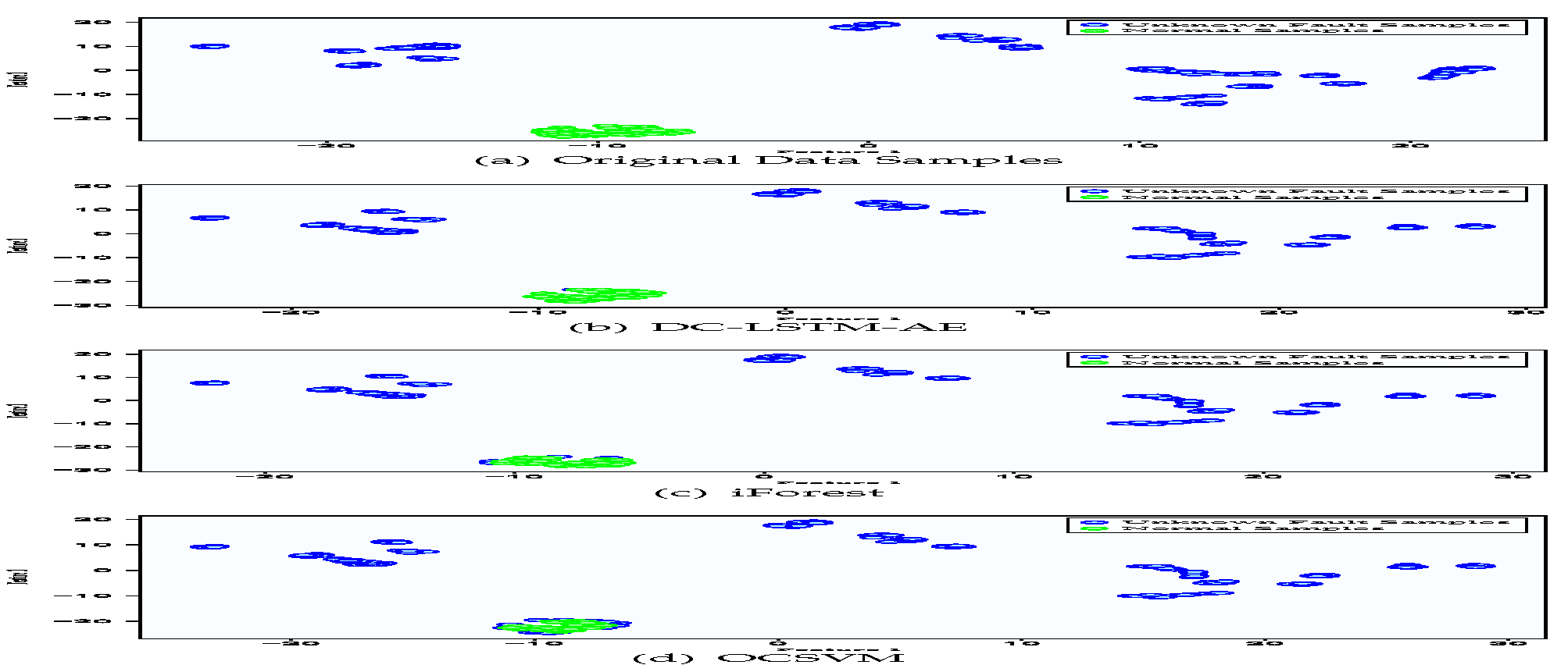
Figure 13.
Unknown Fault Detection Performance of Various Algorithms on Constant-Speed Water Pump Dataset.
Figure 13.
Unknown Fault Detection Performance of Various Algorithms on Constant-Speed Water Pump Dataset.
5. Conclusions
This paper presents a novel mechanical equipment unknown fault detection that addresses the challenge of limited fault samples by training solely on normal samples, enabling accurate detection of unknown faults without relying on fault samples. To overcome the insufficient expressiveness of conventional autoencoders for high-dimensional nonlinear signals, the proposed DC-LSTM-AE model incorporates both CNN and LSTM modules to jointly extract spatial and temporal features, thereby improving its ability to detect unknown faults. The structure of the DC-LSTM-AE model is described in detail, and a mechanical equipment unknown fault detection based on normal samples is designed based on this model, with a detailed elaboration of the detection process for unknown fault samples. To validate the effectiveness of this method, the gearbox dataset from Southeast University and the constant-speed water pump dataset collected from actual factories are selected for experimental validation. Comparative experiments are conducted with traditional autoencoder models and common unknown fault detection algorithms. The experimental results show that the proposed method outperforms other algorithms in multiple metrics for unknown fault detection when only trained on normal samples. Moreover, due to the strong feature extraction capability of the proposed model for samples, it has strong sensitivity and recognition ability for unknown fault samples.
In practical industrial environments, there are often a large number of sensors, and the data types collected by sensors are diverse. Multidimensional data fusion can integrate information from different sensors to improve data integrity and judgment accuracy. Follow-up research will focus on introducing multidimensional data fusion technology into autoencoder networks. Using this technology for feature fusion of different data types can enhance the overall perception ability of autoencoders for equipment conditions, further improving the recognition ability for abnormal or unknown fault samples, and realizing mechanical equipment unknown fault detection based on deep multidimensional data fusion.
References
- Liu, Y.; Chi, C.; Zhang, Y.; Tang, T. 2022. Identification and Resolution for Industrial Internet: Architecture and Key Technology. IEEE Internet of Things Journal. [CrossRef]
- F. Piccialli, N. Bessis, and E. Cambria, “Guest editorial: Industrial internet of things: Where are we and what is next,” IEEE Transactions on Industrial Informatics, vol. 17, no. 11, pp. 7700–7703, 2021. [CrossRef]
- W. Z. Khan, M. Rehman, H. M. Zangoti, and M. K. Afzal, “Industrial internet of things: Recent advances, enabling technologies and open challenges,” Computers & electrical engineering, vol. 81, p. 106522, 2020.
- A. A. Zainuddin, D. Handayani, and I. H. Mohd Ridza, “Converging for security: Blockchain, internet of things, artificial intelligence - why not together,” in 2024 IEEE 14th Symposium on Computer Applications and Industrial Electronics (ISCAIE), 2024, pp. 181–186.
- L. D. Xu, W. He, and S. Li, “Internet of things in industries: A survey,” IEEE Transactions on Industrial Informatics, vol. 10, no. 4, pp. 2233–2243, 2014.
- F. Cao, “Research on machine tool fault diagnosis and maintenance optimization in intelligent manufacturing environments,” Journal of Electronic Research and Application, vol. 8, no. 4, pp. 108–114, 2024.
- J. Sun, J. Liu, and Y. Liu, “A blocking method for overload-dominant cascading failures in power grid based on source and load collaborative regulation,” International Journal of Energy Research, vol. 2024, 2024. [CrossRef]
- C. Arindam and S. K. Ghosh, “Predictive maintenance of vehicle fleets through hybrid deep learning-based ensemble methods for industrial IoT datasets,” Logic Journal of the IGPL, 2024.
- S. Hong, “Advanced data-driven fault detection and diagnosis in chemical processes: Revolutionizing industrial safety and efficiency,” Industrial Chemistry, vol. 10, no. 3, pp. 1–2, 2024.
- H. T. Tai, Y.-W. Youn, H.-S. Choi, and Y.-H. Kim, “Partial discharge diagnosis using semi-supervised learning and complementary labels in gas-insulated switchgear,” IEEE Access, vol. 13, pp. 58 722–58 734, 2025.
- X. Cao and K. Peng, “Stochastic uncertain degradation modeling and remaining useful life prediction considering aleatory and epistemic uncertainty,” IEEE Transactions on Instrumentation and Measurement, vol. 72, pp. 1–12, 2023.
- J. Qi, Z. Chen, Y. Song, and J. Xia, “Remaining useful life prediction combining advanced anomaly detection and graph isomorphic network,” IEEE Sensors Journal, vol. 24, no. 22, pp. 38 365–38 376, 2024.
- K. Choi, J. Yi, and C. Park, “Deep learning for anomaly detection in time-series data: Review, analysis, and guidelines,” IEEE Access, vol. 9, pp. 120 043–120 065, 2021.
- H. Asmat, I. Ud Din, and A. Almogren, “Digital twin with soft actor-critic reinforcement learning for transitioning from industry 4.0 to 5.0,” IEEE Access, vol. 13, pp. 40 577–40 593, 2025.
- J. Zhou, J. Yang, and S. Xiang, “Remaining useful life prediction methodologies with health indicator dependence for rotating machinery: A comprehensive review,” IEEE Transactions on Instrumentation and Measurement, vol. 74, pp. 1–19, 2025. [CrossRef]
- Z.-L. Ma, X.-J. Li, and F.-Q. Nian, “An interpretable fault detection approach for industrial processes based on improved autoencoder,” IEEE Transactions on Instrumentation and Measurement, vol. 74, pp. 1–13, 2025.
- M. Lv, Y. Li, and H. Liang, “A spatial-temporal variational graph attention autoencoder using interactive information for fault detection in complex industrial processes,” IEEE Transactions on Neural Networks and Learning Systems, vol. 35, no. 3, pp. 3062–3076, 2024.
- D. Drinic, M. Novicic, and G. Kvascev, “Detection of lr-ddos attack based on hybrid neural networks cnn-lstm and cnn-autoencoder,” in 2024 11th International Conference on Electrical, Electronic and Computing Engineering (IcETRAN), 2024, pp. 1–4.
- X. Li, P. Li, and Z. Zhang, “Cnn-lstm-based fault diagnosis and adaptive multichannel fusion calibration of filament current sensor for mass spectrometer,” IEEE Sensors Journal, vol. 24, no. 2, pp. 2255–2269, 2024.
- J. Fu, S. Peyghami, and A. N¨²ez, “A tractable failure probability prediction model for predictive maintenance scheduling of large-scale modular-multilevel-converters,” IEEE Transactions on Power Electronics, vol. 38, no. 5, pp. 6533–6544, 2023.
- Z. Wang, W. Shangguan, and C. Peng, “A predictive maintenance strategy for a single device based on remaining useful life prediction information: A case study on railway gyroscope,” IEEE Transactions on Instrumentation and Measurement, vol. 73, pp. 1–14, 2024.
- Y. Lecun, Y. Bengio, and G. Hinton, “Deep learning,” Nature, vol. 521, no. 7553, p. 436, 2015.
- F. Jia, Y. Lei, J. Lin, X. Zhou, and N. Lu, “Deep neural networks: A promising tool for fault characteristic mining and intelligent diagnosis of rotating machinery with massive data,” Mechanical Systems and Signal Processing, vol. 72-73, pp. 303–315, 2016. [CrossRef]
- R. M. Souza, E. G. S. Nascimento, and U. A. Miranda, “Deep learning for diagnosis and classification of faults in industrial rotating machinery,” Computers and Industrial Engineering, vol. 153, p. 107060, 2020.
- T. Han, LongwenYin, and ZhongjunTan, “Rolling bearing fault diagnosis with combined convolutional neural networks and support vector machine,” Measurement, vol. 177, no. 1, 2021.
- Y. Sun, H. Zhang, and T. Zhao, “A new convolutional neural network with random forest method for hydrogen sensor fault diagnosis,” IEEE Access, vol. PP, no. 99, pp. 1–1, 2020. [CrossRef]
- A. Yin, Y. Yan, and Z. Zhang, “Fault diagnosis of wind turbine gearbox based on the optimized LSTM neural network with cosine loss,” Sensors (Basel, Switzerland), vol. 20, no. 8, 2020.
- A. Khorram, M. Khalooei, and M. Rezghi, “End-to-end cnn plus lstm deep learning approach for bearing fault diagnosis,” Applied Intelligence: The International Journal of Artificial Intelligence, Neural Networks, and Complex Problem-Solving Technologies, no. 2, p. 51, 2021.
- J. S. A, D. P. B, and Z. P. B, “Planetary gearbox fault diagnosis using bidirectional-convolutional lstm networks,” Mechanical Systems and Signal Processing, vol. 162.
- M. Jalayer, C. Orsenigo, and C. Vercellis, “Fault detection and diagnosis for rotating machinery: A model based on convolutional LSTM, fast fourier and continuous wavelet transforms,” Computers in Industry, vol. 125, 2020.
- Y. Qiao, K. Wu, and P. Jin, “Efficient anomaly detection for high-dimensional sensing data with one-class support vector machine,” IEEE Transactions on Automatic Control, vol. 35, no. 1, p. 14, 2023. [CrossRef]
- M. S. Sadooghi and S. E. Khadem, “Improving one class support vector machine novelty detection scheme using nonlinear features,” Pattern Recognition, p. S0031320318301663, 2018.
- J. Pang, X. Pu, and C. Li, “A hybrid algorithm incorporating vector quantization and one-class support vector machine for industrial anomaly detection,” IEEE Transactions on Industrial Informatics, vol. 18, no. 12, pp. 8786–8796, 2022.
- X. Song, G. Liu, and G. Li, “An innovative application of isolation-based nearest neighbor ensembles on hyperspectral anomaly detection,” IEEE Geoscience and Remote Sensing Letters, vol. 21, pp. 1–5, 2024.
- C. Li, L. Guo, H. Gao, and Y. Li, “Similarity-measured isolation forest: Anomaly detection method for machine monitoring data,” IEEE Transactions on Instrumentation and Measurement, vol. 70, pp. 1–12, 2021.
- H. Sun, S. Yu, and Z. Li, “Fault diagnosis method of turbine guide bearing based on multi-sensor information fusion and neural network,” IOP Publishing Ltd, 2025.
- H. Ding, K. Ding, J. Zhang, Y. Wang, L. Gao, Y. Li, F. Chen, Z. Shao, and W. Lai, “Local outlier factor-based fault detection and evaluation of photovoltaic system - sciencedirect,” Solar Energy, vol. 164, pp. 139–148, 2018.
- J. Qian, Z. Song, and Y. Yao, “A review on autoencoder based representation learning for fault detection and diagnosis in industrial processes,” Chemometrics and Intelligent Laboratory Systems, 2022.
- S. Plakias and Y. S. Boutalis, “A novel information processing method based on an ensemble of auto-encoders for unsupervised fault detection,” Computers in Industry, p. 142, 2022.
- E. Principi, D. Rossetti, and S. Squartini, “Unsupervised electric motor fault detection by using deep autoencoders,” IEEE/CAA Journal of Automatica Sinica, vol. 6, no. 002, pp. 441–451, 2019. [CrossRef]
- J. Wu, Z. Zhao, and C. Sun, “Fault-attention generative probabilistic adversarial autoencoder for machine anomaly detection,” IEEE Transactions on Industrial Informatics, vol. 16, no. 12, pp. 7479–7488, 2020.
- J. K. Chow, Z. Su, and J. Wu, “Anomaly detection of defects on concrete structures with the convolutional autoencoder,” Advanced Engineering Informatics, vol. 45, no. 3, p. 101105, 2020.
- C. Zhang, D. Hu, and T. Yang, “Anomaly detection and diagnosis for wind turbines using long short-term memory-based stacked denoising autoencoders and xgboost,” Reliability Engineering and System Safety, vol. 222, 2022.
- E. Karapalidou, N. Alexandris, and E. Antoniou, “Implementation of a sequence-to-sequence stacked sparse long short-term memory autoencoder for anomaly detection on multivariate timeseries data of industrial blower ball bearing units,” Sensors (14248220), vol. 23, no. 14, 2023. [CrossRef]
- C. Yin, S. Zhang, and J. Wang, “Anomaly detection based on convolutional recurrent autoencoder for IoT time series,” IEEE Transactions on Systems, Man, and Cybernetics: Systems, vol. 52, no. 1, pp. 112–122, 2022.
- H. Xiang, Aijun Su, “Fault detection of wind turbine based on scada data analysis using CNN and LSTM with attention mechanism,” Measurement, vol. 175, no. 1, 2021.
- D. Zhang, L. Zou, X. Zhou, and F. He, “Integrating feature selection and feature extraction methods with deep learning to predict clinical outcome of breast cancer,” IEEE Access, pp. 1–1, 2018.
- J. Jiao, M. Zhao, J. Lin, and K. Liang, “A comprehensive review on convolutional neural network in machine fault diagnosis,” Neurocomputing, vol. 417, 2020. [CrossRef]
- K. O’Shea and R. Nash, “An introduction to convolutional neural networks,” Computer Science, 2015. [CrossRef]
- T. Mikolov, M. Karafi¨¢t, L. Burget, J. Cernock, and S. Khudanpur, “Recurrent neural network based language model,” in Interspeech, Conference of the International Speech Communication Association, Makuhari, Chiba, Japan, September, 2015.
- Y. Yu, X. Si, C. Hu, and J. Zhang, “A review of recurrent neural networks: Lstm cells and network architectures,” Neural Computation, vol. 31, no. 7, pp. 1235–1270, 2019.
- A. Makhzani and B. Frey, “k-sparse autoencoders,” Computer Science, 2013.
- Z. Chen, C. K. Yeo, B. S. Lee, and C. T. Lau, “Autoencoder-based network anomaly detection,” in 2018 Wireless Telecommunications Symposium (WTS), 2018.
- A. Curtis, T. Smith, B. Ziganshin, and J. Elefteriades, “The mystery of the z-score,” Aorta, vol. 4, no. 04, pp. 124–130, 2016.
- M. A. Panza, M. Pota, and M. Esposito, “Anomaly detection methods for industrial applications: A comparative study,” Electronics (2079-9292), vol. 12, no. 18, 2023. [CrossRef]
- V. D. M. Laurens and G. Hinton, “Visualizing data using t-SNE,” Journal of Machine Learning Research, vol. 9, no. 2605, pp. 2579–2605, 2008.
Figure 1.
DC-LSTM-AE Model Architecture.
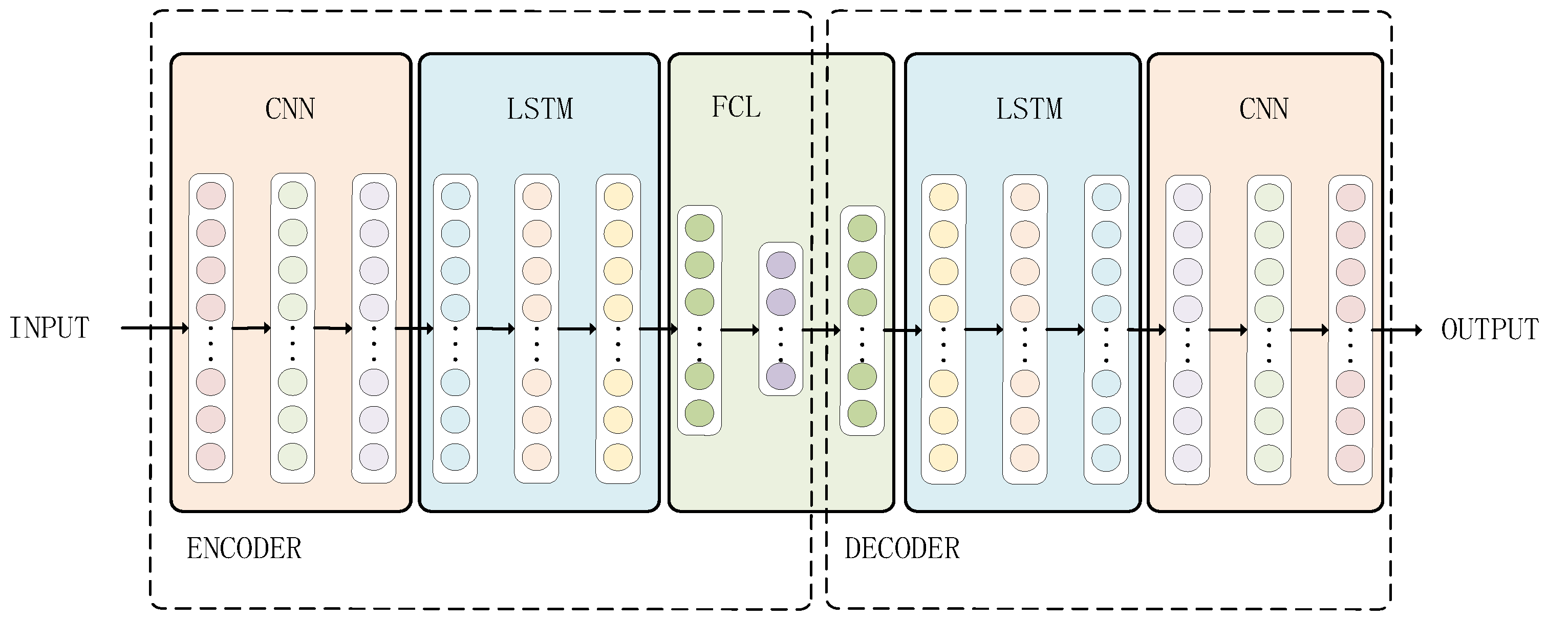
Figure 2.
Structure Diagram of Long Short-Term Memory Network
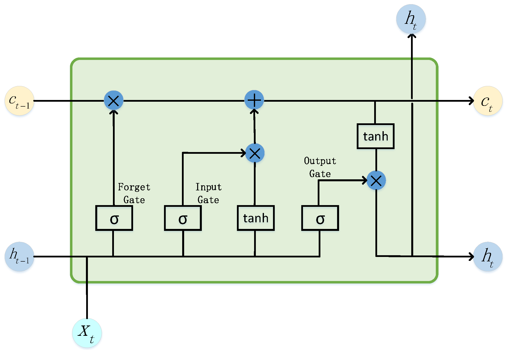
Figure 3.
The Structure of Autoencoder.
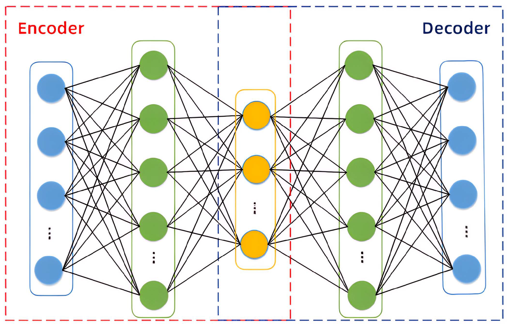
Figure 4.
Mechanical Equipment Unknown Fault Detection Process Based on Normal Samples
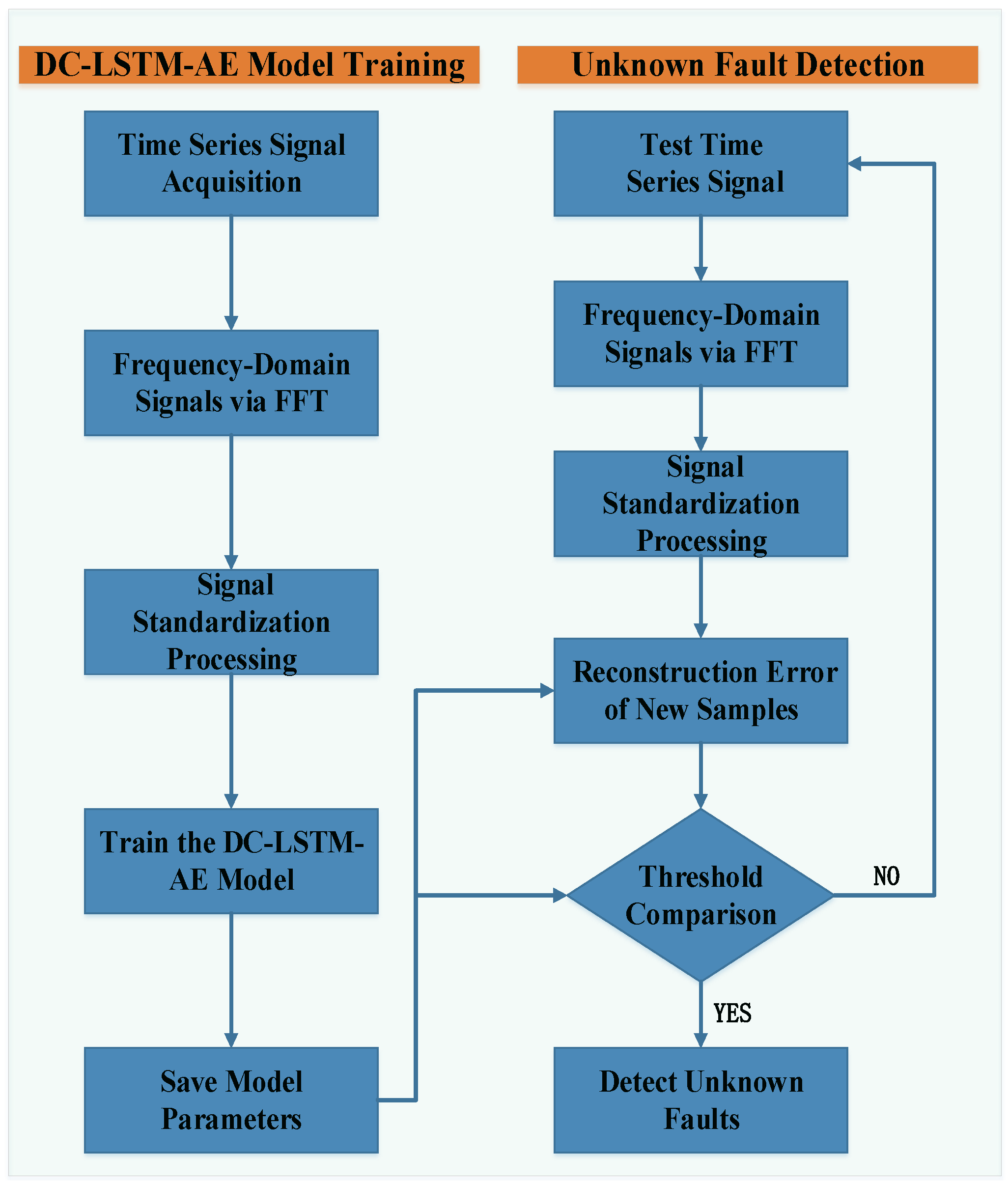
Figure 6.
Reconstruction Error of Test Data for the DC-LSTM-AE Model in the Gearbox Dataset
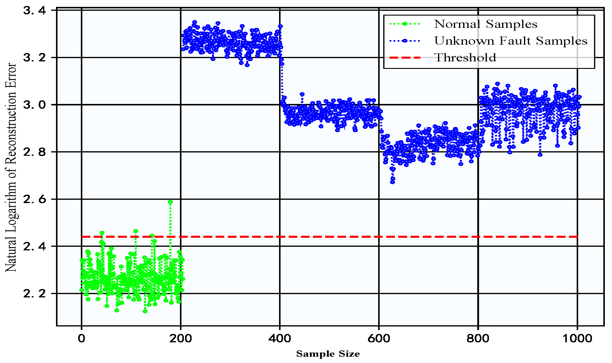
Figure 7.
Reconstruction Errors of Test Data for the AE Model and DCAE Model in the Gearbox Dataset
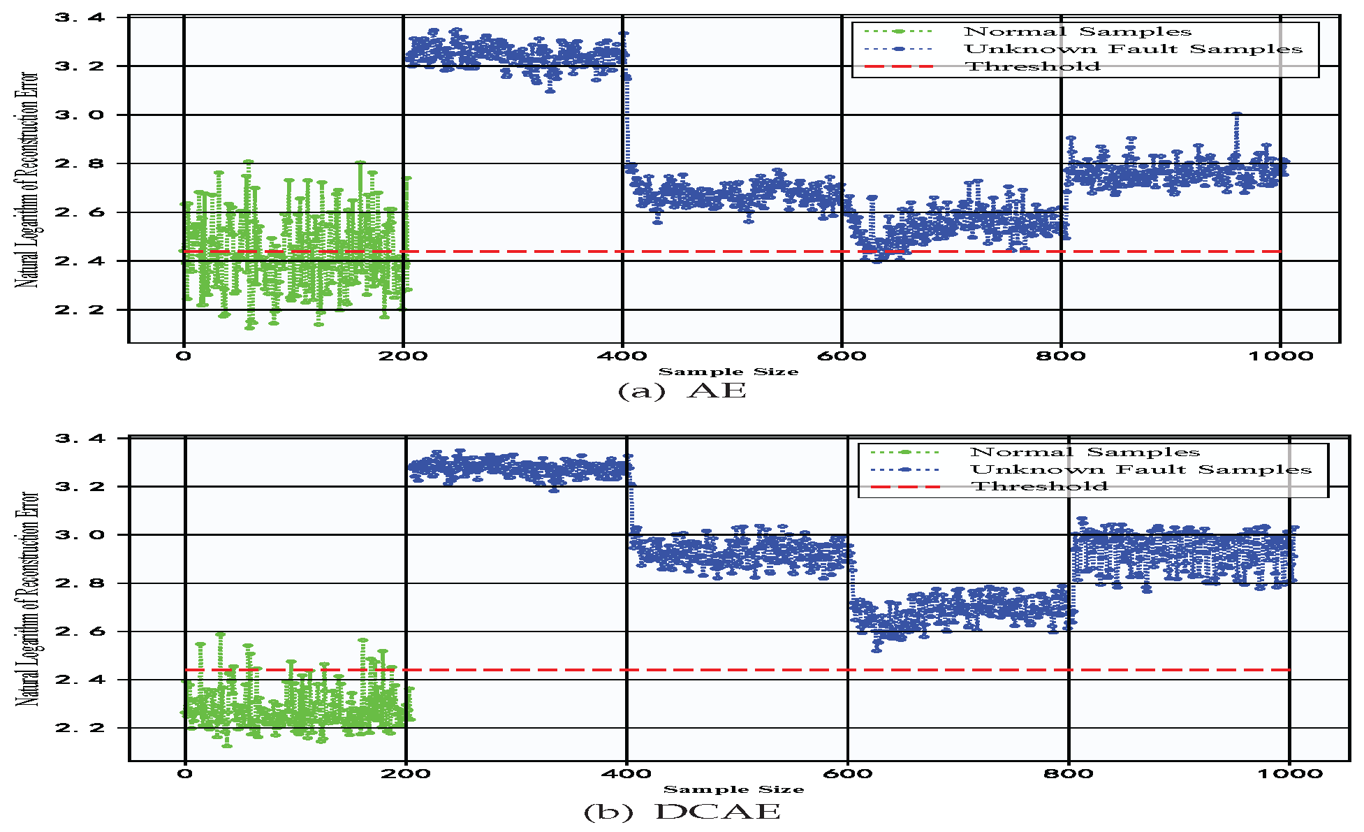
Figure 8.
Detection Results of Different Algorithms for Test Samples in the Gearbox Dataset
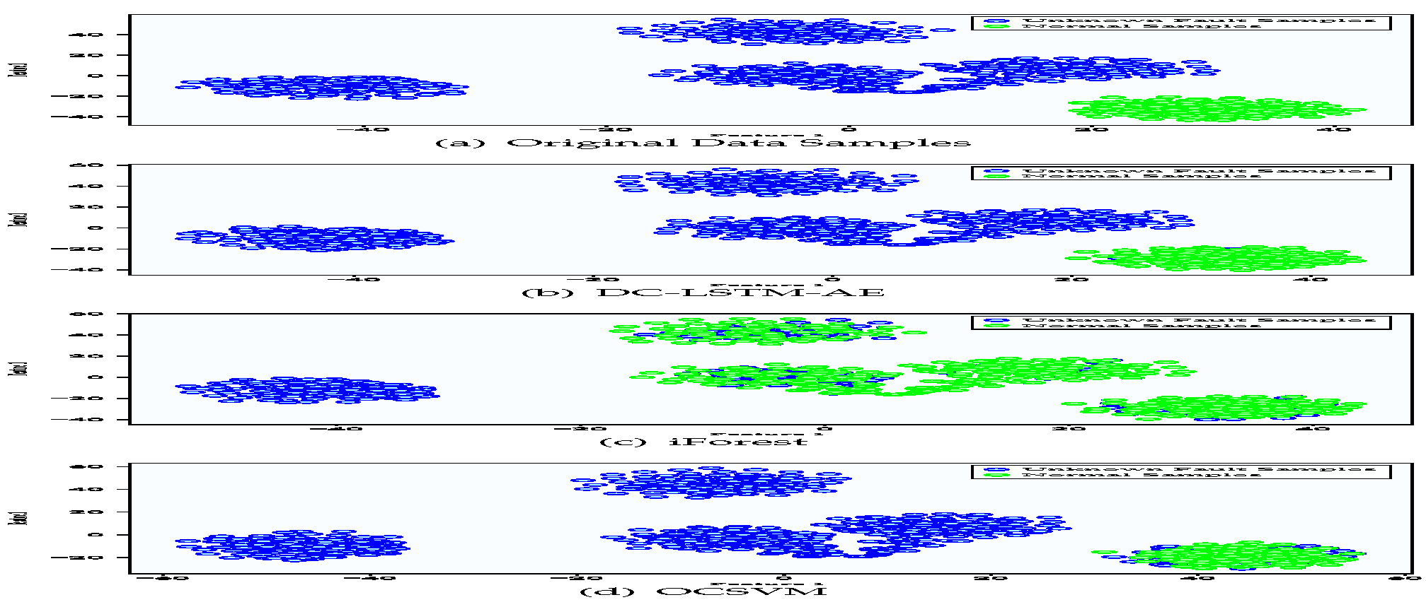
Figure 9.
Unknown Fault Detection Performance of Various Algorithms on Gearbox Dataset
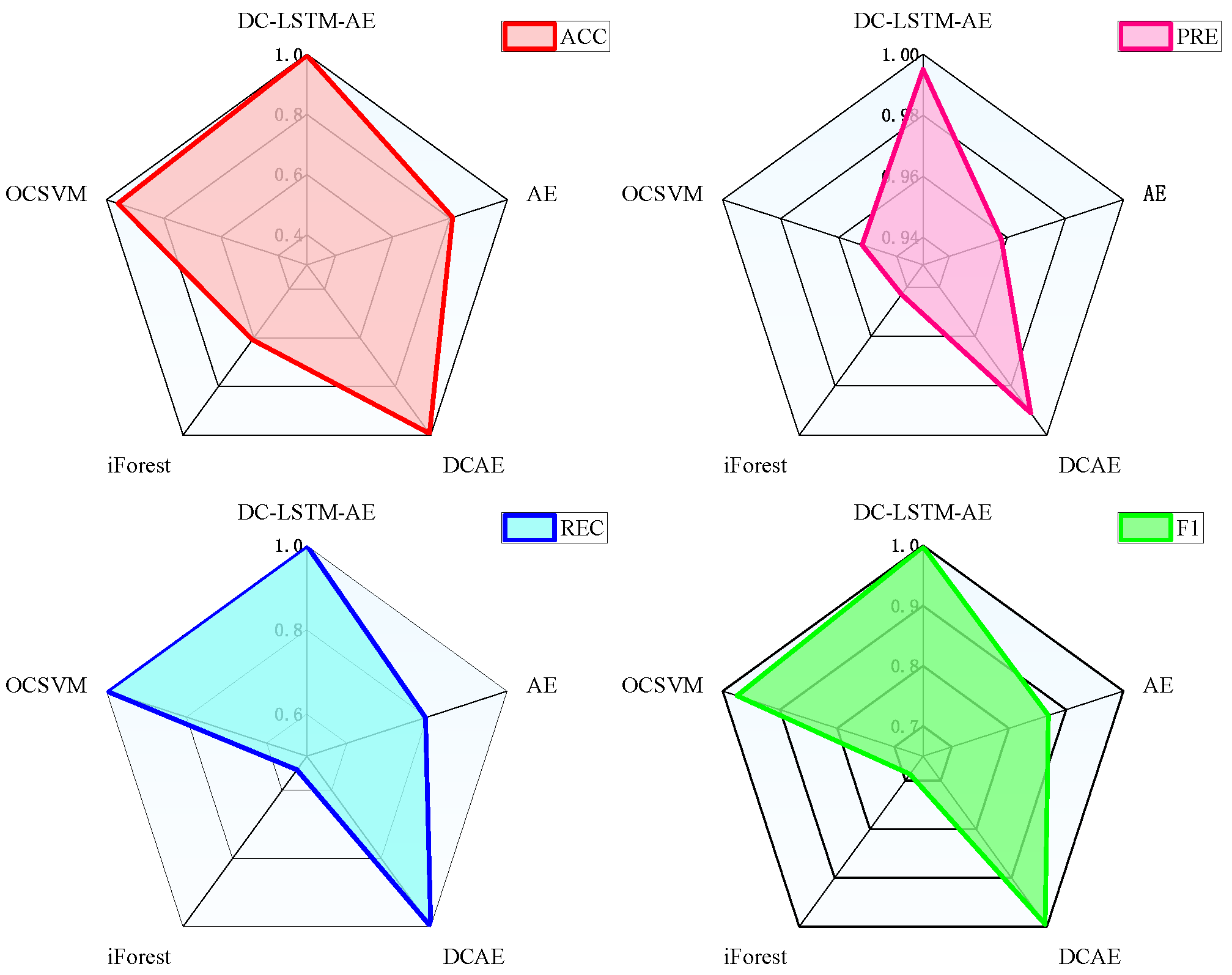
Figure 10.
Reconstruction Errors of Test Data for DC-LSTM-AE Model in Constant-Speed Water Pump Dataset.
Figure 10.
Reconstruction Errors of Test Data for DC-LSTM-AE Model in Constant-Speed Water Pump Dataset.
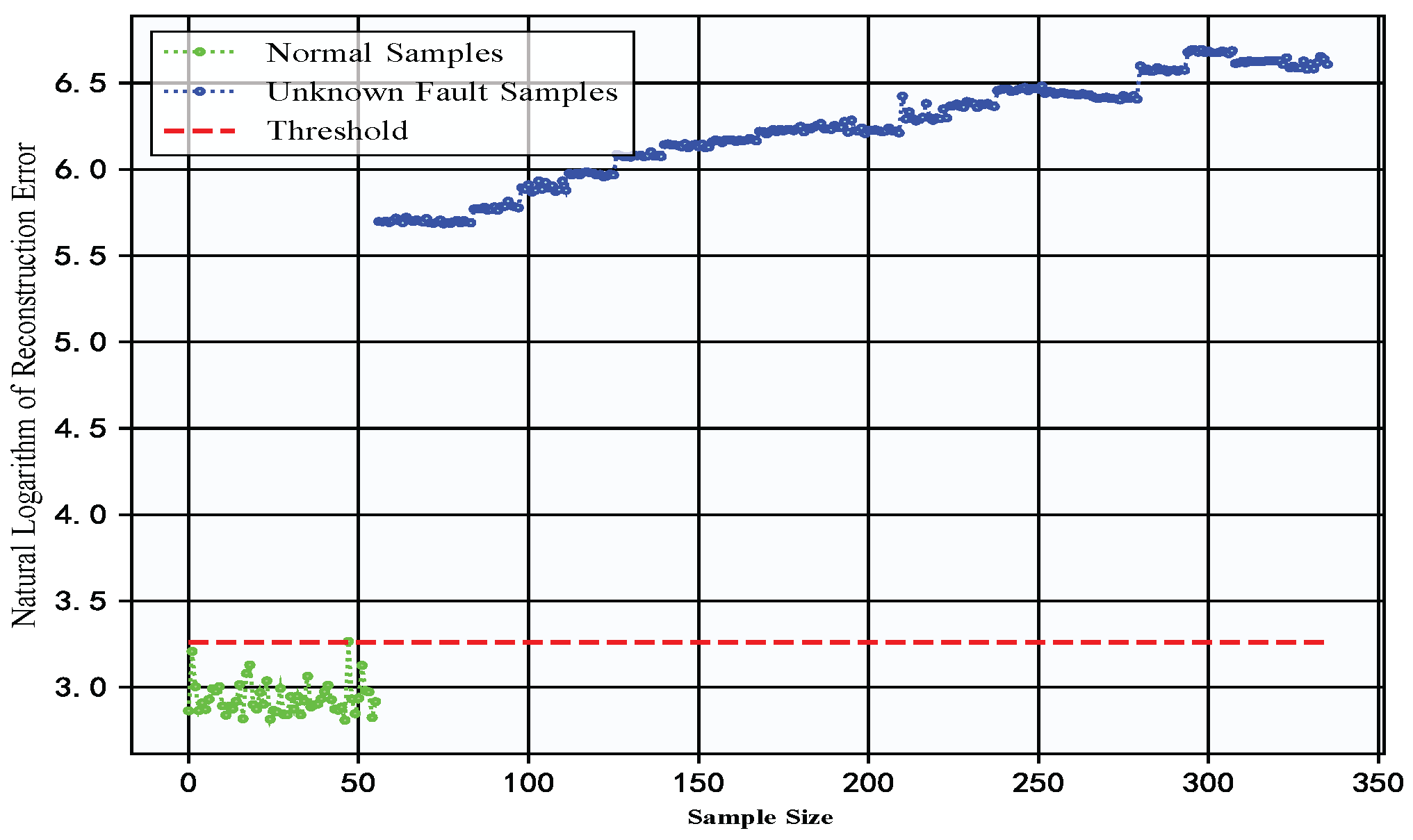
Figure 11.
Reconstruction Errors of Test Data for AE Model and DCAE Model in Constant-Speed Water Pump Dataset.
Figure 11.
Reconstruction Errors of Test Data for AE Model and DCAE Model in Constant-Speed Water Pump Dataset.


Table 1.
Network Architecture of the DC-LSTM-AE Model
| Encoder | Decoder | ||
| Network Layer | Input Dimension | Network Layer | Output Dimension |
| Input Layer | FC Layer 3 | ||
| Conv Layer 1 | FC Layer 4 | ||
| Conv Layer 2 | LSTM Network | ||
| Conv Layer 3 | Deconv Layer 1 | ||
| Conv Layer 4 | Deconv Layer 2 | ||
| Conv Layer 5 | Deconv Layer 3 | ||
| LSTM Network | Deconv Layer 4 | ||
| FC Layer 1 | Deconv Layer 5 | ||
| FC Layer 2 | Output Layer | ||
Table 2.
Dataset Division for Fault Detection Experiment
| Fault Type | All Samples | Training | Testing |
|---|---|---|---|
| Normal | 1022 | 817 | 205 |
| Crack on gear | 200 | 0 | 200 |
| Broken tooth on gear | 200 | 0 | 200 |
| Crack at gear root | 200 | 0 | 200 |
| Wear on gear surface | 200 | 0 | 200 |
Table 3.
Dataset Division for Constant-speed Water Pump Experiment
| Fault Type | All Samples | Training | Testing |
|---|---|---|---|
| Normal | 280 | 224 | 56 |
| Bearing Fault | 280 | 0 | 280 |
Disclaimer/Publisher’s Note: The statements, opinions and data contained in all publications are solely those of the individual author(s) and contributor(s) and not of MDPI and/or the editor(s). MDPI and/or the editor(s) disclaim responsibility for any injury to people or property resulting from any ideas, methods, instructions or products referred to in the content. |
© 2025 by the authors. Licensee MDPI, Basel, Switzerland. This article is an open access article distributed under the terms and conditions of the Creative Commons Attribution (CC BY) license (http://creativecommons.org/licenses/by/4.0/).
Copyright: This open access article is published under a Creative Commons CC BY 4.0 license, which permit the free download, distribution, and reuse, provided that the author and preprint are cited in any reuse.


