
Submitted:
18 July 2024
Posted:
19 July 2024
You are already at the latest version
Abstract
Condition monitoring is a crucial process for ensuring industrial assets' reliability and operational efficiency. In the age of the digital industry, AI-based data-driven condition monitoring is proving extremely effective in detecting potential issues before they escalate into major problems, thereby reducing downtime, minimizing maintenance costs, and extending the lifespan of the equipment. The availability of tools that can enable the operationalization of these data-driven solutions is, therefore, critical. In this direction, this work proposes a comprehensive, modular, and scalable pipeline covering all the steps from the data acquisition to the AI model training and inference phases. The tool integrates the data acquisition and processing steps with a configurable feature extraction phase. Moreover, the system also integrates deep learning algorithms for diagnosis and prognosis, including a domain adaptation stage to permit transfer learning and increase generalizability. In addition, it features a communication system using MQTT, which allows for an online data stream to enable real-time monitoring and maintenance. The overall infrastructure was deployed in actual industrial settings and tested in a real-time experiment, demonstrating the proposed approach's validity.
Keywords:
data pipeline
; predictive maintenance
; condition monitoring
; domain adaptation
; fault diagnosis
; remaining useful life estimation
1. Introduction
The digital industry revolution, driven by the development of technologies for extracting value from data, has led to the emergence of Condition Monitoring (CM) as a fundamental pillar of the sector. Predictive Maintenance (PM) employs CM techniques to plan maintenance activities strategically, with the objective of preventing critical unexpected downtimes in a controlled industrial plant. PM draws upon data-driven insights to identify patterns and anomalies, thereby enabling the prediction of potential issues at an early stage.
AI-based strategies are increasingly gaining popularity over traditional methods, predominantly based on empirical observations and regular equipment inspections. The former has proven to be more reliable and accurate and can guarantee higher levels of automation and scalability.
Such approaches in industrial applications, however, typically require the processing of a substantial volume of heterogeneous data in real-time, in addition to the implementation of reliable and general models to provide accurate indications of the state of the machinery. Nevertheless, the performance of algorithms can be significantly degraded by the presence of bottlenecks at any point in the flow.
With all the new algorithms proposed yearly, which claim competitive performance, industries must invest time and resources in setting up ad hoc experiments to test their efficiency in a specialized environment. Therefore, the availability of a general and stable framework that is easily portable across different machines and allows domain experts to quickly implement modern solutions and find the most suitable for their needs becomes even more crucial.
This work proposes a comprehensive, modular, and scalable data pipeline that integrates all the stages of a complete CM workflow. It encompasses data acquisition and processing steps, a configurable feature extraction phase, and the possibility of deploying the developed deep learning models.
The modular structure ensures high flexibility of the data stream, as the different modules can be modified and recombined according to the user’s specific problem. Finally, the setup is available for offline simulation over historical data and real-time signal monitoring in a dynamic environment.
Unlike other works, this approach incorporates several analysis and processing strategies and guarantees new users maximum compatibility to integrate new setups and models easily.
The pipeline was developed in collaboration with an Italian gearbox manufacturer, and its efficacy was subsequently evaluated through a series of experiments on the test bench, designed to reproduce real-world gearbox stress and degradation accurately. The proposed pipeline implements deep learning models for the two principal tasks of predictive maintenance: fault identification and breaking point forecasting. Additionally, it incorporates the most common domain adaptation algorithms, which enable the transfer of domain knowledge across different machines, thereby aiding the model’s learning.
While the models’ performances will be presented in the text for completeness, we want to stress that this work focuses primarily on the full solution that moves from the ingestion of the data to the adaptation of the algorithms and the final predictions of the models.
This paper is structured as follows. First, in Section 2, we review some state-of-the-art analyses and present related works of similarly designed data pipelines in the industrial field. Then, in Section 3, we extensively analyze the structure proposed by accurately describing the distinct modules, including its real-time processing workflow, which is deepened in Section 4. Subsequently, the pipeline is validated on a real-world case study in Section 5. Finally, possible future updates are suggested in Section 6, and conclusions are drawn in Section 7.
2. Related Works
Traditional approaches to predictive maintenance predominantly rely on engineering analysis of the physical systems, necessitating a detailed examination of system components and operational parameters to identify in advance potential failures. As a result, these frameworks are largely concentrated on analyzing the sensors implemented in the system and establishing thresholds for the acquired signals to differentiate between normal and anomalous behaviors [1,2]. In recent years, domain experts in the field of industrial condition monitoring have increasingly turned to data-driven approaches over model-based methods. This is because, in the former, no underlying physical knowledge of the engineering system is required [3]. However, this assumption is based on the premise that the background knowledge can be replaced with machine and deep learning algorithms, an operation that is often not straightforward. Several publications [4,5] underscore the critical role of research within data pipelines. Although this aspect may be considered secondary to the development of models, it remains essential when models need to be used in a production environment. Research in this area predominantly addresses common issues encountered across different setups and explores optimal strategies for their resolution. This paper incorporates such an analysis, mostly based on the case study detailed below, and approaches these problems by employing methods that are as generalizable as possible, thereby allowing the framework to be adaptable to different contexts.
Many solutions have been developed and proposed to provide a general framework for automating the most common workflows, encompassing the data processing stages and tuning hyperparameters in models. Nevertheless, most of those were designed to address the aforementioned scenario, characterized by a scarcity of machine learning experts.
An illustrative example is provided by the TPOT project (Tree-based Pipeline Optimization Tool) [6] and its subsequent updates [7] and [8]. TPOT is presented as a tool for automating signal processing and machine learning tasks, designed to be fully automated and accessible to non-experts in the field. It leverages genetic programming and Pareto optimization to maximize classification scores on a reference dataset.
In the AUTORUL [3] project, automatic feature extraction and model selection are integrated with fine-tuned standard regression methods to adapt the pipeline for prognostic tasks. However, this approach appears overly simplistic and too limited when applied to complex predictive maintenance problems.
Neuroimage analysis, with pipelines like FastSurfer [9], appears to share a common approach with predictive maintenance. Neuroimaging, as PM, faces the problem of dealing with large datasets and, therefore, follows similar workflows.
In PipeDream-2BW [10], the primary objective is to enhance parallelization and acceleration, providing a dependable solution to the configurations in which large models are executed in low-memory setups. This is achieved by meticulously distributing the operations across the available devices. It is acknowledged that the hardware available for predictive maintenance is often a limiting factor in the analysis process. The monitored components are designed to operate reliably for several years under normal working conditions. However, maintaining a real-time setup with a continuous data stream can become prohibitively expensive when multiple new-generation devices are involved. Consequently, we have proposed a set of models with minimal hardware requirements for the training and inference phases while maintaining satisfactory performance. Our objective has been to balance time/memory efficiency and cost sustainability optimally.
To meet all realistic scenario requirements, we propose MoPiDiP (MOdular real-time PIpeline for machinery DIagnosis and Prediction), a tool that guarantees customization and scalability. It is intended to be used semi-supervised by professionals who seek solutions for R&D and production tasks.
3. Pipeline Organization
The processing workflow proposed in this paper is organized in a data pipeline composed of several independent blocks. Each block is designed to implement functions and utilities covering the most common data processing steps, which can be personalized and recombined according to needs. The aim is to provide a solution that seamlessly integrates with different machine setups and allows a degree of customization to accommodate data-driven models and processing requirements. Given the variability of sensor installations, the different data formats they produce and all the possible end usages of the devices, the robustness of the structure is a priority, also to account for common disruptions like signal downtimes and human interventions. The modular structure, with independent, customizable, and recombinable blocks, provides sufficient flexibility to adapt to different machine configurations. The setup has been explicitly evaluated for industrial gearbox diagnosis and prognosis, and it is primarily intended to handle condition monitoring tasks, both online and offline.
The general planned workflow of the data management part is summarized in Figure 1.
The initial section of the pipeline (Section 3.1) encompasses all the building blocks designed for data management and preparation. It directly communicates with the sensors to supervise the acquisition and loading of raw data. It implements the most common signal processing techniques to extract and prepare relevant features that will be employed by the models. The final step of this section entails preparing the data for the domain adaptation phase, whereby the samples are split and normalized into the assigned domains.
Following this preprocessing stage, the subsequent module supports the extraction of supplementary anomaly detection indices (Section 3.2). It employs both well-established machine learning tools and autoencoder-like models, which facilitate the extraction of features that are more domain-independent.
The final blocks of the structure (Section 3.3–Section 3.5) are dedicated to the design and implementation of two general deep-learning models that can address prognostics and diagnostics tasks. Due to the variability of the problem, novel domain adaptation techniques are adopted to enhance the ability to generalize to unforeseen situations and machines, frequent problems in real-world scenarios.
The pipeline’s modular design allows users to safely incorporate new custom steps into the infrastructure without modifying existing blocks. This feature enables, for instance, the transition to an online mode via a simple plugin. This plugin communicates with the sensor data stream to save intermediate files that are compatible with the format required by the first block, thus permitting the standard workflow through the rest of the pipeline.
The following Sections will examine each module in detail, elucidating its functionality and its role within the infrastructure. Additionally, delving into the technical aspects, the resilience of each block with respect to common disruptions in real machine environments will be demonstrated.
3.1. Data ETL
The first part of the infrastructure covers the fundamental data ETL (Extract, Transform, and Load) operations. Skipping the transmission of data by the sensors, which will be explored in the “online section" (Section 4), three fundamental blocks can be identified within this first preprocessing stage:
- Signal Extraction
- Features Extraction
- Domain Splitting
The high level of modularity of this infrastructure allows for the isolation and utilization of each pipeline component separately. Indeed, the project was realized with the objective that different users should be able to reassemble the blocks according to their specific needs and the machine setup. The only requirement is rigorous control of the input and output data formats throughout the flow, as incompatibilities may result in the generation of undesirable errors and behaviors. Moreover, as a stable solution for an industrial setup, the pipeline is designed to operate with a fair number of heterogeneous experiments even simultaneously. For this reason, folders, file names, tags, and versioning are required to follow a strict hierarchical structure with a clearly defined internal nomenclature. This enables the user to run multiple evaluations.
3.1.1. Signal Extraction
The monitoring of industrial systems is often characterized by the presence of many sensors that collect and dispatch variables of diverse types and meanings, each with its own acquisition rate. Collecting all this information, HDF5 is among the most effective data formats since it allows storing large amounts of heterogeneous data in a hierarchical structure [11]. Although the memory access is not optimal, this format ensures high flexibility, particularly for real-time acquisition and mapping. Finally, it permits the dynamic introduction of new channels without necessarily affecting existing stable operations.
The expected internal key structure of the HDF5 files is "sensor" → "channel" → "RAW/PreProcess" → "Timestamp". This approach ensures the potential for transmitting diverse signals from the same sensors and accounts for the possibility of preliminary operations performed directly by the devices. Metadata pertaining, for example, to the acquisition time, working conditions, and sample rate can be embedded directly within the structure as independent channels.
Since data transmission is not always continuous, dividing the signal into multiple “sessions" is advisable. These are defined as data periods containing multiple time windows of arbitrary length, called “acquisitions". The length of both sessions and acquisitions may vary according to the characteristics and operational routines of the observed machine. This solution is initially developed to address the occasional downtimes of the devices involved, minimizing the consequent loss of data chunks. Additionally, it permits mitigating storage costs for large data collection periods at high frequencies.
The extraction of meaningful information from the HDF5 files is achieved by looping over all available sessions and creating Python objects containing both the signals and metadata of each acquisition window. As a result, one binary Pickle [12] dump file is generated for each individual session. Also, while the HDF5 files contain the entire set of signals transmitted by the sensors, after this step, only the required variables are sent to the subsequent modules, significantly reducing the dataset dimension.
In offline mode, when multiple acquisition files are available, the signal extraction phase can be accelerated by enabling multiprocessing, which launches jobs that run in parallel for each HDF5. Nevertheless, this feature is disabled by default in order to prevent an increase in the hardware requirements for this infrastructure.
Aware of common practices in industrial environments, the pipeline needs to be robust to periodic changes in the machine setup. To enhance its flexibility, the configuration allows for the possibility of providing a customized set of input channels. This is achieved by providing a simple JSON file [13], which allows the user to reassign all the default channels with the new nomenclature employed by the sensors. This ensures the pipeline’s operativity even with new devices. The online procedure (Section 4) provides a dedicated mapping of the channel streams, which can reproduce intermediate HDF5 files with the same structure, thus easily connecting to the rest of the pipeline. This step is of critical importance for scalability. If different data sources are provided, developing an ad-hoc plugin to connect the new signals to the default key structure and proceed with the flow-through will be sufficient. On the other side, the usage of Pickle files enables an initial unfolding of the larger HDF5 files and the elimination of redundant or unnecessary variables.
The pipeline has been tested using data from various sources, including accelerometers (vibration), thermometers (temperature), multimeters (current, voltage), and field buses (speed, torque). Such data was sampled at high (25 kHz) and low (1 Hz) frequencies. The procedure is described in a general manner, as it must be applicable to all types of signals collected by the sensors. However, the literature [14,15,16] clearly shows that vibrational signals are the most informative in the context of predictive maintenance for rotating systems.
3.1.2. Feature Extraction
The second block of the pipeline encompasses the entire feature extraction stage. In predictive maintenance focusing on diagnostics and prognostics of rotating machinery, most state-of-the-art models necessitate a preprocessing step aimed at extracting significant features that more accurately reflect the degradation status of the observed component. The binary files generated in the previous stage contain the time series associated with the sensors’ measurements, organized in sessions, sorted by acquisition time, and with the associated metadata. The module, iterating over each file, extracts all the single acquisition objects within the sections and further fragments them into non-overlapping sub-acquisition windows of parametrically adjustable length. This procedure ensures a higher number of samples available and equal-length sub-signals, thus generating more consistent features across the entire dataset.
The preponderance of the developed functions has been designed explicitly for analyzing vibrational signals, given their superior informative value in condition monitoring tasks. Information brought by other variables, such as the device temperature or the operational velocity of the apparatus, can also be incorporated into the models, for example, through statistical representation (average, standard deviations).
Digital Signal Processing (DSP) is a crucial tool in extracting meaningful features from the signals acquired by the sensors. The effectiveness of predictive maintenance is heavily reliant on the relevance of this information, as these meaningful features serve as the building blocks for predictive models, providing valuable insights into the health and performance of the machinery. These features can encompass various characteristics, including frequency-domain analysis, time-domain analysis, statistical measures, and spectral analysis. Consequently, selecting variables that most accurately reflect the deterioration of the apparatus’s operational regime represents a critical stage in formulating maintenance strategies. The pipeline implements the most common features provided by DSP, that have been used, in the years, as condition indicators for some kind of tasks affine with condition monitoring ([14,15,17,18]). For simplicity, they are grouped by output dimensionality.
The actual list of one-dimensional features implemented is:
- -
- Time-Domain Statistics
- -
- Wavelet Packet Energy
- -
- Hilbert-Huang
- -
- Kurtogram statistics
- -
- Wavelet statistics
- -
- Frequency-domain statistics (from the power spectrum)
- -
- Rolling Mean, Variance, RMS
Most 1-dimensional features consist of statistics (mean, variance, maximum, peaks, etc.) extracted from the transformed signal. In this way, the meaningful content of the signal is preserved and compressed in a few informative variables.
The actual list of two-dimensional features implemented is:
The module also supports the extraction of complex-valued features, like the Short-Time-Fourier-Transform ([23,24]), of which one can take the magnitude or continue with non-real-valued operations. The raw signal can be treated as a feature in itself and carried forward without additional processing, as many recent transformer-based models claim high performances when taking in input time series ([25,26]). Alternatively, rolling variables (the pipeline implements rolling mean, rolling variance, and rolling mean-square) can represent a good trade-off between maintaining the time series structure and, at the same time, compressing the information stored in the data.
The module also implements some canonical filters to be applied to the signal before processing. They could help reduce the noise or remove undesired frequencies:
Another functionality implemented in the block is automatically managing gaps in the signals. Given that data acquisitions and transmissions are not always synchronized and stable, the acquisition objects created in the preceding block are monitored and, if necessary, realigned to preserve the dataset’s coherence and avoid missing or duplicate samples. Finally, the pipeline enables the signal to be downsampled to a lower frequency before feature extraction [31]. This allows the results to be aligned across sensors with different sampling rates and facilitates the comparison of the results achieved on a narrower spectrum. The features extracted from each sub-acquisition window are reformatted as dictionary-like objects and saved as binary files. This approach ensures the scalability of the pipeline even with heterogeneous data. The extraction phase is completely configurable, allowing for the inclusion of specific features or parameter variations tailored to each experiment. Additionally, the two cases of diagnosis and prognosis may require separate setups, and thus, they are handled independently. A metadata file is compiled to maintain a log of the domain-specific details of every acquisition, with one entry for each distinct binary file. The hardware requirements may vary contingent upon the specific features selected, with higher memory consumption requisite for tasks involving images, like spectrograms or nested plots, compared to those involving sparser or one-dimensional variables. Nevertheless, the resultant files from this phase serve more of a transient purpose, as they will be subject to recombination and rescaling in the subsequent step. Consequently, under strict constraints on the available memory, these files could theoretically be deleted post-processing yet remain recoverable from the original HDF5 files.
For the case study presented below in Section 5, better prediction performances were obtained considering MFCC, Time-Domain Features, and Rolling RMS of the signal.
3.1.3. Splitting
The third and final block of the ETL part of the pipeline deals with the final preparation and organization of the samples just before the training and inference modules of the models. The main objective of this Section is to arrange a dedicated setup for the various domain adaptation algorithms (Section 3.3), which are the final part of the infrastructure. Consequently, the previously extracted features are organized into source and target sets, each including train, validation, and inference subsets.
The splitting step, which is fully configurable, allows the train-validation-test division to be defined by either stating the percentage or the exact number of hours of data that should be added to each subset. Furthermore, the pipeline automatically assigns the "healthy" or "faulty" labels to the samples indicated for diagnosis tasks. The module copies the files into the appropriate subfolder and updates a metadata file with the new destination path. This allows the pipeline to keep track of the files and recombine them in multiple source-target combinations.
Duplicating all files is not an optimal storage solution. However, this approach can be beneficial in guaranteeing the best performance from the actual setup when working with heterogeneous data and running multiple experiments. In real-time monitoring, data generated within this block can be deleted right after being used by models to free up space.
Once per experiment, a normalization object is fitted on a custom portion of the dataset and then used to rescale all the upcoming features.
Among the methods implemented, the most common choices are standardization and min-max scaling. These practices have allowed a successive memory-friendly data-loading step during the model training and inference phases. In industrial applications, sensors often collect data for very long periods; thus, the possibility of efficiently selecting and loading the samples assumes high relevance. A more detailed discussion of domain adaptation algorithms is presented later in the paper.
3.2. High-Level Feature Extraction
A common and straightforward approach to fault detection tasks is to compare signals’ features with some reference thresholds, which may be obtained from literature or earlier studies ([32,33]). However, direct confrontation may be deceptive because signals are frequently acquired in different dynamic situations or from different devices or sensors.
In the presented framework, an intermediate module provides an alternative linkage between the low-level features extracted by the ETL stage and the models implemented afterward. The objective is to provide a novel set of more domain-independent variables that could enable a more fair comparison. Furthermore, integrating these higher-level features may reduce the workload for subsequent diagnostic and prognostic algorithms by supplying new data that are more compressed, more sensitive to changes in the machine’s health, and, therefore, better suited for anomaly detection tasks. It is still possible to feed features such as raw signals or time-frequency representations, like MFCCs, directly into the models by simply skipping this block. However, this may compromise the scalability of the solution, especially in situations where an extended period of data acquisition or a demanding transfer learning step is required.
In the tested solution, autoencoders were selected to provide greater abstraction in the feature engineering process. An autoencoder is an artificial neural network designed to learn efficient latent representations of data, typically by reducing the input’s dimensionality and capturing the most relevant features. Composed of a pair encoder-decoder, autoencoders are trained via backpropagation to minimize a reconstruction loss, typically a mean-squared error between the input and its reconstruction. Autoencoders have been well established in the literature for anomaly detection tasks and are widely used also in the area of condition monitoring [25,34,35]. The solution implements a Multi-Variational Autoencoder (MultiVAE) model, a composite architecture that processes the different feature channels from the preceding modules, automatically adapting to their types and dimensions. Additionally, the MultiVAE is designed to enhance the information content of the lower-level features, thereby providing a more accurate reflection of the machine’s degradation status at the subsequent stages of the pipeline.
As the name suggests, the architecture employs three different categories of autoencoders:
- -
- -
- a Convolutional Autoencoder for two-dimensional features (MFCC, Fourier transforms, spectrograms) [36];
- -
The training procedure and the network’s primary parameters are entirely customizable. At the same time, the pipeline automatically selects the optimal architecture, depending on the collection of selected features generated by the earlier stages. The complete MultiVAE setup workflow is shown in Figure 2.
The model employs the features extracted from the signals as independent channels to generate a compressed latent representation of the input data. The latent space is deliberately formed of a limited number of variables, thereby enforcing the compression of the information contained in the input. Typically, only data from the experiment’s initial period, comprising samples still deemed "healthy" status, are utilized to train the model. From this perspective, the model can be conceptualized as a denoising autoencoder, capable of recognizing artifacts in the healthy features but gradually losing its generalization capabilities beyond this working point. As the machine status gradually deteriorates, the characteristics retrieved by the vibration signal start to deviate from stable conditions, accumulating more noise. Therefore, the changes in the latent space can be used as a reliable measure of this degradation and exploited for anomaly detection. Empirical evidence suggests that the most effective variable for replicating this decline is the model’s reconstruction loss, whose gradual deterioration across the machine’s lifetime is clear in the examples reported in the scheme Figure 2.
Autoencoders ensure enhanced operational efficacy, particularly in terms of hardware requirements. In support of this consideration, the technical details of the implemented architectures, the training phase, and the devices utilized in the case study experiments are presented in Appendix A. These models exhibit a contained parameter count and are designed to learn only from a portion of the data, typically spanning the initial hours of the experiment. This allows the training phase to be run completely offline, which is particularly useful in scenarios characterized by stringent online device constraints. The updated network’s weights can be deployed within a lightweight online setup. Portability is, in fact, another of the main qualities of this pipeline. Finally, autoencoders facilitate the compression of high-dimensional features, such as the frequently used MFCCs, into subsets of variables rearranged in tabular formats, expediting successive domain adaptation steps and drastically reducing the memory requirements.
In the development stage, autoencoders’ architectures were engineered to overfit the training dataset on purpose. This strategy aimed to compress input information of a healthy configuration, leveraging the divergence of points in the latent space and the reconstruction error as metrics for assessing health degradation. Notably, a small latent space leads to an efficient latent representation, enhancing model sensitivity to deviations in system health.
To enhance the resilience of diagnostic and prognostic models, the pipeline facilitates the incorporation of anomaly detection indices with the variables generated by the autoencoders. Over the years, numerous machine learning algorithms have been developed to identify irregularities and deviations from “ordinary conditions". The pipeline integrates some general and common methodologies, allowing users to increase the number of signals connected with the machinery’s health status degeneration. The available methods include One-Class SVM [38], Local Outlier Factor [39], Isolation Forest [40] and Elliptic Envelope [41], which can be applied to either the signal itself or the latent space of the autoencoders.
Each experiment is processed separately within this pipeline block, and the final features are eventually combined, rearranged, and gathered to create a distinct tabular dataset that ensures a compressed depiction of the monitored component’s health condition.
In the forthcoming case study (Section 5), the MultiVAE model has been exclusively employed for the prognosis task, combining the compressed latent representation of MFCCs, time-domain features, and rolling RMS values from the vibration signal (as detailed in Section 3.1, paragraph Feature Extraction). The novel tabular data were constructed utilizing the reconstruction errors of the three autoencoders and their respective latent variables. Conversely, within the diagnostic problem, the original MFCCs underwent direct processing without intermediary compression, accordingly undergoing the domain adaptation phase.
As previously articulated, industrial applications necessitate an approach that accommodates their inherent diversity and specificity, precluding the application of a singular, universally applicable methodology. It is crucial to remark that this paper does not want to delineate an optimal strategy for resolving condition monitoring tasks; rather, it focuses on presenting a flexible and complete framework. This objective is complemented by a validation conducted in a real-world scenario, for which a valid and reliable solution is presented.
3.3. Domain Adaptation
The final module of the pipeline contains the models implemented to fulfill tasks of diagnosis and prognosis of the machinery’s health status (the complete workflow is summarized in Figure 3).
One of the main challenges inherent in industrial systems lies in the distinctive nature of each possible setup configuration. The unique attributes encompassing operational modalities, mechanical component heterogeneity, variability in consumption and utilization, and sensor acquisition disparities further underscore each setup’s individuality. One approach to mitigate this challenge involves conducting comparative analyses with a designated reference experiment characterized by a well-documented lifespan. PM models can attempt to project this information onto the new monitored setup by extrapolating insights derived from this reference scenario. Consequently, the incorporation of domain adaptation techniques becomes essential in the development of a trustworthy and general solution [42,43].
Domain adaptation (DA) is a subcategory of transfer learning, providing algorithms and techniques designed to address the common problem in which the distribution of data used for training a model (source domain) differs from the distribution of data where the model is deployed (target domain). In a monitored system, the accuracy of predictive models is often compromised because the source domain, typically represented by historical data or simulated environments, diverges substantially from the operational context. Domain adaptation will facilitate the seamless knowledge transfer, thereby mitigating performance degradation and enhancing generalization capabilities across heterogeneous domains.
Finally, domain adaptation promotes the optimization of resource utilization and cost-effectiveness by eliminating the need for domain-specific model retraining in the target operational context.
This work encompasses some of the most common deep learning domain adaptation algorithms, re-adapted from the PyTorch implementation proposed in the public GitHub repository "DeepDA" [44]. The authors presented their work as a lightweight, extendable, and easily learnable toolkit that precisely met the needs of the pipeline. Aware of the rapid development in Condition Monitoring, it would have been impractical to include a unique solution in the infrastructure, given the frequency with which new frameworks are proposed. Consequently, the pipeline incorporates a few general and well-established algorithms while remaining flexible and adaptable to setup-specific routines or emerging innovative architectures.
The fundamental infrastructure of the DA module involves essentially three networks:
- -
- a Transfer Network, the main core of the setup, implements the transfer rule and produces a latent high-dimensional representation of the input data;
- -
- a Domain Discriminator, to learn distinguishing the sample domain (source or target);
- -
- a Predictive Model, focused on learning the main task (a classifier for diagnosis problems and a regressor for prognosis ones).
This simple design facilitates the implementation of several DA algorithms proposed in recent literature while concurrently accommodating user-defined optimization functions or case-specific transfer networks. At the time of this paper’s composition, the repository hosts two adversarial-based algorithms: Domain-Adversarial Neural Networks [45] and Dynamic Adversarial Adaptation Networks [46]. These algorithms, operating at the training level, aim to map input variables onto a shared latent space, rendering target samples indistinguishable from labeled source samples. Other techniques, such as Maximum Mean Discrepancy (MMD [47]), Correlation Alignment for Unsupervised Domain Adaptation (CORAL [48]), Batch Nuclear-norm Maximization (BNM [49]) and Local MMD (LMMD [50]), on the other hand, are metric-based procedures and endeavor to minimize specific loss functions to align features originating from distinct domains. For those, the Domain Discriminator is usually replaced by artefacts within the cost function. Moreover, the proposed module accommodates a multi-source modality, wherein training batches are assembled proportionally by mixing samples from various reference experiments. This approach is anticipated to enhance information exchange in scenarios characterized by the availability of multiple data sources.
The backbone of the transfer learning infrastructure is designed to be versatile, supporting both diagnosis and prognosis tasks. A detailed discussion of specific use cases will be provided in subsequent Sections, while in what follows, the main focus is on the domain adaptation step.
The considered feature set comprises a combination of the high-level variables generated by the MultiVAE (Section 3.2), alongside the features extracted from the raw signals through digital signal processing operations. The former should be more helpful in this context, as they have been designed to be more domain invariant. Nevertheless, since each machine is processed independently, a transfer learning step can still help map the insights obtained from historical data to the ongoing experiment.
In the case study discussed later, the Domain-Adversarial Neural Network emerged as the most proficient algorithm for exploiting vibration signals. Here, the transfer network functions as a novel feature extractor aiming to align the latent spaces of the source and target domains through its transfer loss, rendering them indistinguishable. In operational terms, these networks were trained simultaneously but with different learning rates, minimizing a composite loss function comprising the regressor’s mean-squared error and the discriminator’s cross-entropy. Further details of the employed architectures, parameters, and training methodologies are provided in Appendix A.
Selecting an appropriate source domain is a crucial step within condition monitoring applications, significantly influencing the accuracy and validity of predictive outcomes. Without a universal criterion, the choice hinges upon empirical validation. The overarching strategy involves selecting an experiment that closely mirrors the monitored machine’s mechanical attributes and usage dynamics, guided by any available prior information. This approach should facilitate the transfer of knowledge between coherent environments. In industrial contexts, to ensure adequate preparation for new components to be monitored, it is imperative to organize a diverse array of experiments, encapsulate a wide spectrum of configurations, and be able always to provide a reliable set of source data (as in the case presented in Appendix B).
Another advantageous aspect of employing this domain adaptation framework is its minimal hardware demands, in continuity with the objectives of the autoencoder-based feature extraction methodology outlined in Section 3.2. In addition to the modest parameter count of the neural networks involved (Appendix A), the training phase occurs only once, after the initial data collection phase of the target experiment. In a manner analogous to the MultiVAE model, the initial data samples obtained pertain to a system still in a healthy condition, thus establishing a baseline for the machine status.
An alternative approach could have been the periodic retraining of the domain adaptation model in a continuous learning framework as new data arrive. Nonetheless, in the context of real-world components, monitoring operations may persist for extended durations, potentially spanning years, resulting in a substantial accumulation of large volumes of data, necessitating prolonged training times and increased hardware prerequisites. Moreover, different kinds of machine utilization and consumption could exacerbate model performance degradation, compounded by the absence of a standardized labeling protocol for newly acquired samples.
Consequently, it is believed that adopting a lightweight yet reliable and portable setup is imperative. This approach significantly diminishes the duration of simulations and tests, obviating the need for a progressive retraining process. It also cuts the costs associated with periodic data transmission and storage. Furthermore, online operations are reduced to only model inference and forecasting tasks by conducting the training phase offline on dedicated hardware.
3.4. Fault Diagnosis
In industrial system monitoring, the topic of fault detection and diagnosis, namely locating and understanding the underlying cause of anomalies or malfunctions in a system, is crucial. Accurately identifying parts of a complex apparatus that exhibit abnormal behavior enables timely intervention and remediation, thereby helping to prevent machine downtimes, increase dependability, and avoid costly system failures.
Most of the features extracted in the stages described until this point can be used to indicate anomalies in the sensor measurements, at least in comparison with a baseline of ordinary behavior. In the case study under consideration, the optimal strategy was to rely on the MFCC (Section 3.1) of the vibration signal. The feature extractor network comprised one-dimensional convolutional and linear layers in this case. Although the model required two-dimensional features, the preprocessing step involved computing the mean value across the rows to reduce the fluctuation of the features in the time domain and to focus the analysis on the frequency domain. Further technical details regarding the training phase and the architecture are provided in the Appendix A. Fault diagnosis often involves different techniques, varying according to the monitored component or available sensors. This pipeline implements a dedicated module that reframes the problem as a classification task, thereby enabling the generalization to new experiments by applying the domain adaptation algorithms presented in Section 3.3.
The implementation requires a set of source case studies composed of samples collected (and processed) from healthy and faulty conditions. A class represents each condition, and the classifier is trained to distinguish such classes. The classifier is trained using the adversarial domain adaptation framework in which the hidden features generated by the healthy part of the target experiment are aligned with the healthy hidden features of the source sets.
Being set up as an anomaly detection classifier, the algorithms can also be trained offline, with the initial "healthy" hours of the monitored experiment providing the model with the baseline conditions. During the inference phase, in online running, the module outputs two fundamental metrics:
- the classification probability of the new features representing a healthy configuration or one of the known fault classes;
- the relative risk, defined as the ratio between the current probabilities the diagnosis model returned and those observed during the training phase.
As a machine component gradually deteriorates, the pipeline is expected to warn users about the specific part presenting anomalies. This is achieved by returning, for each acquisition, a vector of probabilities associated with the different health conditions. Conversely, the values associated with the healthy class will inevitably decline over time due to the inevitable consumption. An illustrative example of typical behavior extrapolated within a real-world experiment is presented in Figure 4, which depicts a typical scenario ending with the pinion breaking. As the test progresses, it becomes evident that the probability associated with the healthy class declines while the values connected with the classes of the faults increase. Among these, the pinion class emerges as the most prominent, as evidenced by the relative risk on the right. A detailed explanation of the case study is provided subsequently in Section 5.
3.5. RUL Estimation
Machine health prognostics is the other area of research in this context. Unlike diagnostics, prognostic models take a step further by predicting the potential evolution of a device’s damage over time, enabling timely interventions to prevent costly downtimes and maintain operational reliability. By leveraging predictive techniques, prognostic models can anticipate and warn about potential failures, optimize maintenance strategies, enhance safety, and increase the machine lifespan in industrial plants. Prognostic models are designed to provide reliable estimates of the future state of a system based on its current condition and operational history. They also allow the forecasting of critical parameters such as the Health Index (HI) and the Remaining Useful Life (RUL) [51,52], which are indicators of the health status of the component being actively monitored.
From an operational standpoint, the prognostic model implemented in the pipeline is based on the same domain adaptation backbone described in Section 3.3. The setup employs domain adversarial learning to train a regressor on one or more complete run-to-failure sources. This enables the model to learn from the machine’s entire lifespan, thereby enhancing its capability of mapping the observed features’ anomalies to reliable health index values. The input variables are typically comprised of a combination of Digital Signal Processing features (Section 3.1) and MultiVAE (Section 3.2) features. However, training a regressor requires a characterization of the source information. In the absence of a general and objective strategy to label the training samples, empirical observations have led to the hypothesis of a linear degradation, which appears to represent a satisfactory approximation over time. Consequently, each feature in the source set is assigned a corresponding Health Index value in the interval [1,0], inversely proportional to the running time of the experiment. This behavior is then transferred to the target latent space during the domain adaptation phase, essentially enforcing the trends of the target features to collapse on such linearity and providing a punctual estimate of the Health Index for the new samples. As previously outlined in Section 3.3, the model’s training during real-time monitoring necessitates only the target experiment’s initial “healthy" hours to deceive the discriminator in an adversarial learning setup. In contrast, the regressor is trained exclusively with the labeled source samples. The final state of the architecture should comprise a regressor model capable of functioning indiscriminately across the two domains, thereby enabling the generation of a punctual health index estimate during the forward pass.
The number of remaining useful hours until machine failure can be estimated by analyzing the general trend of the Health Index for an ongoing experiment. This is achieved by re-adapting, in the pipeline, a robust open-source forecasting algorithm, such as Facebook Prophet [53], to support breaking-point prediction. Model predictions can show high fluctuations in real-world data, which is often characterized by large amounts of noise and discontinuities. Consequently, simple forecasting approaches such as linear interpolations can be problematic and misleading if used without further consideration. To overcome this problem, the proposed solution adopts Prophet [53] to extrapolate the RUL. According to its documentation:
“Prophet is a procedure for forecasting time series data based on an additive model where non-linear trends are fit with yearly, weekly, and daily seasonality, plus holiday effects. It works best with time series with strong seasonal effects and several seasons of historical data. Prophet is robust to missing data and shifts in the trend and typically handles outliers well.”
To our knowledge, no previous research has exploited this algorithm for condition monitoring applications, as it is primarily designed to analyze trends in economic contexts. However, even if machinery vibrations cannot be commonly considered seasonal data, the robustness of the model to the common frequent changes in the Health Index appears appropriate for this task. Furthermore, as the lifespan of industrial machines is commonly several years long, the algorithm could detect periodicity (or seasonality) in usage and maintenance and exploit this information to improve accuracy.
This choice is contingent on the case study and is not guaranteed to be the optimal solution for all configurations and setups. However, as the pipeline is designed to function in different environments, it allows for the parallel implementation of several alternatives, thereby enabling a fair comparison of the different methods. Potential alternatives to Prophet, depending on the type of machine and data the user will be working with, include:
Figure 5 depicts an illustrative example of the anticipated behavior of the forecasting algorithm at a specific point in the operational lifetime of the monitored device. It also serves as a comprehensive display of the machine’s status, offering immediate insights to the technician responsible for the pipeline. A detailed description of the scenarios in the image, with a quantitative analysis of the experiments analyzed, is provided in Section 5.
4. Online Processing
One of the key advantages of this pipeline is its adaptability, which allows for the recombination of all the modules described with ease. A plugin has been developed to facilitate the execution of the aforementioned modules in an online setting, with data acquisition facilitated through an MQTT broker and real-time processing. MQTT is a widely adopted transmission protocol in industrial applications, offering robustness and reliability in low-bandwidth networks [56].
For companies, the availability of a framework capable of operating seamlessly in both offline and online modalities holds considerable significance. Online processing assumes importance because it simplifies portability and guarantees remote management capabilities such as real-time monitoring and alerting.
The online procedure has been designed to be scalable and low-memory demanding, thus suitable for deployment on an edge computing model (technical specifications of the hardware employed are reported in Appendix A). Condition monitoring can run for several years and necessitates balancing the costs of data transfer and storage. The data stream is rarely continuous, a more common setup consists in sending periodic fix-sized acquisitions that can be loaded, processed and then discarded, to preserve space. As previously discussed in Section 3.2 and Section 3.3, the models require only an initial training phase that can run completely offline. Consequently, the model’s weights can be deployed at run-time, and the inference phase can be reduced to the last independent period of data without necessarily reloading the whole experiment. That’s a very convenient strategy that optimizes hardware usage.
The initial stage of the online version of the pipeline is the data acquisition step. Upon the beginning of an online experiment, the pipeline collects a specified number of hours, which are subsequently utilized as a training set for the models. Afterward, the pipeline proceeds to the inference phase for each subsequent acquisition. Following the real-time data processing and feature extractions, the pipeline interrogates the trained models and transmits the predictions through the MQTT broker for diagnostic and prognostic activities. The modular architecture of the pipeline affords scalability across various communication channels for result dissemination, including dashboards and real-time databases. Furthermore, the pipeline incorporates a set of recovery protocols to address potential interruptions, such as preserving the pipeline’s operational state to facilitate resumption from a specific execution juncture in the event of failure. Another notable characteristic entails parallelizing the operations of the models within non-blocking parallel threads. This approach ensures that computationally intensive tasks executed by the models do not impede the workflow of the pipeline, instead functioning autonomously within distinct instances.
An online functioning pipeline is a fundamental block of a condition monitoring framework.
5. Gearboxes Case Study
The pipeline has been developed over three years in collaboration with a leading company specialized in producing gear motors, drive systems, planetary gearboxes, and inverters [57]. The project’s final objective was the definition and realization of predictive maintenance algorithms for fault diagnosis and prediction for their products and clients. Such collaboration enabled the development of the pipeline within a real-world setting, with partial control of the environment and of the experimental conditions.
A total of forty-eight tests were conducted during the project duration, with datasets collected from five different gearbox families (coaxial gearboxes, planetary gearboxes, angular axes, worm-type gearboxes, and parallel axes) and covering most common usages and configurations. These experiments were characterized by dynamical lifespans resulting from different mechanical loads, rotational speeds, prototypes, and interventions. The tests can be divided into two categories: endurance experiments, which evaluate the predictions of the prognostic model, and "healthy-faulty" experiments, in which damage to the system was artificially simulated and sensor measurements were recorded in damaged and non-damaged cases. In Appendix B, a few examples of the different deterioration patterns observed in the gearboxes illustrate the wide range of different dynamics the model had to support.
The diagnosis setup employed artificially simulated faults to collect vibration signals from healthy and faulty machinery. Five possible damage scenarios were considered for the main components of gearboxes: solar, pinion, crown, bearing, and unbalance. The diagnostic model returns each class’s corresponding probability of occurrence and relative risk.
Given that industrial devices are typically assumed to last for many years under normal load conditions, the data acquisition period was reduced to just a few months by accelerating the experiments by removing lubrication or increasing speed and torque beyond nominal usage. This approach allowed for the collection of reliable data for the lifetime of many devices. Additionally, technicians performed maintenance during the tests to extend their duration and simulate a real-world environment. The model could often independently capture such interventions, showing a local increase in the health index immediately after. Another advantage of testing the algorithms in real-time experiments is that less prevalent issues may be encountered in the offline setup. Interruptions to the data stream can lead to complications in the continuous predictions of the models, particularly in instances where the system is idle. Still, the sensors continue to transmit (noisy) data. The pipeline demonstrated resilience in correctly identifying and handling these situations, logging the downstream periods, and excluding them from the analysis and processing phases.
Figure 4 and Figure 5, which have already been presented, depict an actual example of the return values of the pipeline after the inference tests. The former image represents the results predicted by the diagnosis model in an endurance experiment conducted in April 2022. The test was conducted on a coaxial gearbox, and the pinion broke after just a few days due to installation problems. The model employed as a reference source a dataset from the historical archive relative to another coaxial gearbox covering three fault classes (bearings, pinions, crowns). It is evident that, as expected, the risk associated with the component sustaining significant damage gradually increased over time, while the probability associated with the healthy state decreased. With this prediction available, the technicians could have terminated the trial before the sudden failure of the machine, potentially identifying the installation error and preventing further costly maintenance. The second image presents an example of the prognostic algorithm for an endurance experiment conducted between June and September 2023. The source was a coaxial gearbox, while the target was an angular gearbox. Figure 5 provides an overview of a model prediction near failure. As previously explained in Section 3.5, Prophet provides a forecast of the Health Index returned by the model, from which the estimated breaking point of the machine can be extrapolated as the intersection between the prediction and the x-axis. The remaining useful life is the number of hours until that point. The algorithm also returns a confidence interval, which can be set depending on the task, that can be exploited to define a corresponding range for the punctual prediction . The algorithm has been designed to raise two warnings, "yellow" and "red," in correspondence with the Health Index dropping below the thresholds of 10% and 5%, respectively. The former warning indicates that the gearbox is heavily damaged and requires replacement. In contrast, the latter warning indicates that the machine is approaching a catastrophic failure and should immediately cease operation to prevent further damage. Numerically, a red warning often corresponds to a RUL prediction of 0 hours.
For completeness, the performances obtained regarding RUL estimation are presented and discussed in Appendix B for some of the cases. In conclusion, the configuration was scalable, efficient, and cost-effective regarding hardware requirements, including storage, processing, training, inference, and transfer times.
6. Future Works
The pipeline and implementation presented in this paper proved to be a robust and scalable solution for diagnosis and prognosis in industrial applications. Its modular architecture facilitates seamless module substitution, contingent upon adherence to input/output format specifications.
For instance, emerging domain adaptation methodologies, including multi-source domain generalization approaches, are poised to replace the existing ones.
Furthermore, as previously mentioned in Section 3.5, additional techniques should be investigated in HI forecasting and RUL estimation, such as incorporating approaches based on Long Short-Term Memory networks. Such integration could guarantee more reliable estimates of the RUL of the observed component. Moreover, the pipeline’s reliance on the manual selection of source experiments, practiced according to the characteristics and operations of the target entity, underscores the imperative of integrating domain expertise. Consequently, the proposed methodology assumes a hybrid stance between model-based and data-driven approaches. The pipeline may implement various automatizations to extract domain knowledge from the solution, including unsupervised source set selection and automatic parameter tuning for the models. Such enhancements could empower non-expert users to obtain reliable machine health estimates, even without comprehensive domain familiarity.
7. Conclusions
In this paper, we address one of the main problems faced by modern industries: the necessity of real-time processing of large volumes of data to develop reliable algorithms that provide accurate representations of machinery status. As presented in Section 2, the majority of the existing solutions are entirely automatized and addressed to non-experts in the machine learning area, thereby limiting the potential for those seeking more configurable solutions to address their specific problems and for those who wish to keep up with the latest developments in the field of predictive maintenance. We have designed a comprehensive, modular, scalable data pipeline, integrating the data acquisition and processing steps with recent deep learning solutions to the most common condition monitoring tasks. Furthermore, the various functions are guaranteed to be composable, and the possibility of minimizing online operations is guaranteed, thereby promising minimum hardware requirements. As reported in Section 5, the pipeline has been tested on many real-world experiments (both in an offline and online fashion) planned by Bonfiglioli, a leader company in the gearbox production, confirming the technical characteristics planned for. Furthermore, these examinations demonstrated the software’s robustness and adaptability in addressing the most prevalent issues encountered in a real-world setting. Despite not being the paper’s primary focus, we present how the models have been implemented and validated in a realistic environment, yielding satisfactory outcomes in fault diagnosis and remaining useful life estimation tasks. Additionally, it has been demonstrated that forecasting algorithms, such as Prophet, could play a pivotal role in condition monitoring, providing further motivation for future research endeavors.
Author Contributions
Conceptualization, M.C. and A.G.; methodology, M.P., A.G. and P.S.; software, D.C and M.P; validation, M.P. and D.C.; formal analysis, M.C.,P.S.; investigation, M.P.; resources, M.P. and D.C.; data curation, M.P and D.C; writing—original draft preparation, M.P.; writing—review and editing, M.C., A.C., P.S. and M.C.; visualization, M.P and D.C; supervision, M.C., A.G and P.S.; project administration, M.C.; funding acquisition, M.C. All authors have read and agreed to the published version of the manuscript.
Funding
This research received no external funding.
Data Availability Statement
The data that support the findings of this study are the property of Bonfiglioli SPA [57], which supported the research. Due to the proprietary nature of the data, they are not publicly available. Researchers who wish to access the data for replication or further study should contact the company manager to discuss the possibility of access under appropriate confidentiality agreements and conditions.
Acknowledgments
These testing activities have been supported by Bonfiglioli SPA, within the financed project “AIoTBonfiglioli“ n° 01/17, funded by Trentino Sviluppo. The aim of the project was the creation of an Industrial IoT platform based on algorithms that combine model based reasoning with artificial intelligence dedicated to the realization of Bonfiglioli IOT devices aimed at enhancing the Bonfiglioli commercial offer. Furthermore, the tests were carried out in a test center designed and built as part of this project at the Bonfiglioli site in Rovereto.
Conflicts of Interest
The authors declare no conflicts of interest. The funders had no role in the design of the study; in the collection, analyses, or interpretation of data; in the writing of the manuscript; or in the decision to publish the results.
Abbreviations
The following abbreviations are used in this manuscript:
| AI | Artificial Intelligence |
| DL | Deep Learning |
| PM | Predictive Maintenance |
| CM | Condition Monitoring |
| DA | Domain Adaptation |
| DSP | Digital Signal Processing |
| MFCC | Mel Frequency Cepstral Coefficients |
| multiVAE | Multiple Variational Autoencoder |
| LSTM | Long short-term memory |
| MQTT | Message Queuing Telemetry Transport |
| MoPiDiP | MOdular real-time PIpeline for machinery DIagnosis and Prediction |
Appendix A. Training Details
The pipeline was designed to run the algorithms implemented on the iMX8 ARM 64 bit [58] edge computing setup. The hardware made available 2GB of RAM and 16 GB of eMMC, part of which was reserved for the installation of the requisite packages. As the features are processed in real-time, the effective storage required can be reduced to the space occupied by the features of a single acquisition window, which can be freed just after the inference step. A proper setting of the batch size can help regulate the RAM used. During the experiments, the training processes were performed using no more than 2 GB, thanks to the low parameter count of the models.
Table A1 details the complexity of the various models employed and summarizes the dimension of input and output variables of this specific setup.

Table A1.
Complexity of the architectures
| Model | N parameters | Size parameters | Input shape | Output shape |
| VAE | 5978 | 0.03 MB | (11,) | (11,) |
| ConvVAE | 20183 | 0.22 MB | (39,50) | (39,50) |
| LSTMVAE | 50497 | 0.23 MB | (1,30) | (1,30) |
| Health Index Regressor | 117746 | 0.48 MB | (192,) | (1,) |
| Fault Classifier | 566889 | 2.27 MB | (100,) | (4,) |
The MultiVAE architectures have been trained with an Adam optimizer, with a learning rate oscillating between and , according to a cyclic scheduler. The weight decay of the regularization has been set to , and the latent spaces of the autoencoders have been reduced to just 2 latent units. In a machine with a NVIDIA V100 gpu and 8 GB of RAM, the training times of the three architectures can vary from a few minutes (one-dimensional VAE) to a few dozen (especially for the convolutional networks). The actual numbers largely depend on the amount of data used, both in terms of sampling frequency and number of hours collected.
Appendix B. Bonfiglioli Experiments
A multitude of data was collected throughout the project, under different working conditions, for a range of apparatus and subject to different load cycles.
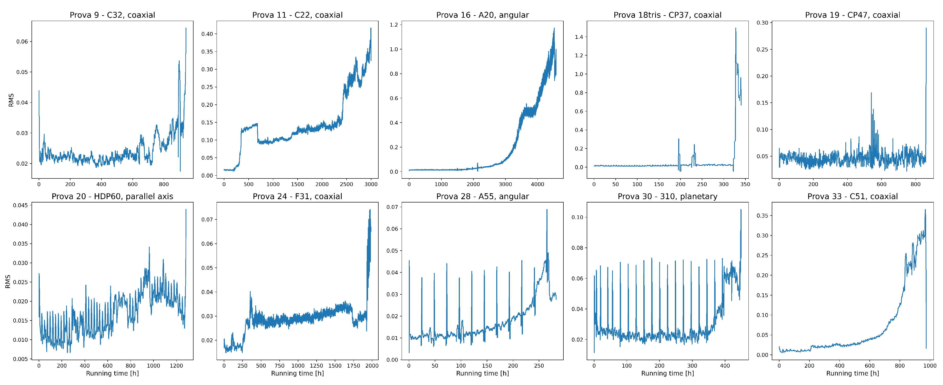
As illustrated in Figure A1, which depicts the Root-Mean-Square (RMS) of the signal for some of the experiments, the dynamics exhibited by the system can be disparate. In some cases, the vibrations seem to remain stable until the end of the device’s operational life, while in others the consumption appears to be more gradual over time. In yet others, local oscillations are observed as a result of regime changes or maintenance work. The pipeline developed and the models implemented were designed to guarantee optimal and balanced performance in most cases, ensuring solutions that were independent of environmental conditions.
Figure A1.
RMS of the Bonfiglioli experiments analyzed.
Finally, in Table A2, some numerical results related to the prognosis experiments obtained with the forecasting model described in Section 3.5 are reported. The commissioner was satisfied with the results achieved as they guaranteed to raise meaningful warnings, potentially enabling prompt maintenance that could have delayed the breakup of the gearbox.
Table A2.
Some results of Bonfiglioli experiments.
| Source | Target | Target Duration [h] | First Warning [h] | Second Warning [h] | ||
|---|---|---|---|---|---|---|
| RUL (true) | RUL (pred) | RUL (true) | RUL (pred) | |||
| 9 (coaxial) | 14 (planetary) | 150 | 30.53 | 45 [0,95] | 5.05 | 0 [0,0] |
| 9 (coaxial) | 28 (angular) | 280 | 17.53 | 70 [0,-] | 2.01 | 0 [0,0] |
| 9 (coaxial) | 18 (coaxial) | 350 | 126.09 | 45 [0,-] | 54.71 | 0 [0,0] |
| 33 (coaxial) | 15 (angular) | 550 | 47.81 | 0 [0,95] | 18.72 | 0 [0,70] |
| 15 (angular) | 11 (coaxial) | 2200 | 396.21 | 382 [166,-] | 278.17 | 0 [0,22] |
This table contains the results achieved with the RUL model for some of the Bonfiglioli experiments. The column "RUL (true)" contains the exact remaining life of the machine (a posteriori) when the warning was raised, while "RUL (pred)" contains the model’s exact prediction with the corresponding confidence interval (when the interval is half open we assume that the upper extreme is higher than 30 days).
References
- Metje, N.; Chapman, D.; Walton, R.; Sadeghioon, A.; Ward, M. Real time condition monitoring of buried water pipes. Tunnelling and Underground Space Technology 2012, 28, 315–320. [Google Scholar] [CrossRef]
- Zhao, Y.; Liu, Z.; Zhang, H.; Han, Q.; Liu, Y.; Wang, X. On-line condition monitoring for rotor systems based on nonlinear data-driven modelling and model frequency analysis. Nonlinear Dynamics 2024, 112, 5229–5245. [Google Scholar] [CrossRef]
- Zöller, M.A.; Mauthe, F.; Zeiler, P.; Lindauer, M.; Huber, M.F. Automated Machine Learning for Remaining Useful Life Predictions. 2023; arXiv:cs.LG/2306.12215]. [Google Scholar]
- Raj, A.; Bosch, J.; Olsson, H.H.; Wang, T.J. Modelling Data Pipelines. 2020 46th Euromicro Conference on Software Engineering and Advanced Applications (SEAA), 2020, pp. 13–20. [CrossRef]
- Munappy, A.R.; Bosch, J.; Olsson, H.H. Data Pipeline Management in Practice: Challenges and Opportunities. Product-Focused Software Process Improvement; Morisio, M., Torchiano, M., Jedlitschka, A., Eds.; Springer International Publishing: Cham, 2020; pp. 168–184. [Google Scholar] [CrossRef]
- Olson, R.S.; Bartley, N.; Urbanowicz, R.J.; Moore, J.H. Evaluation of a Tree-based Pipeline Optimization Tool for Automating Data Science. CoRR, 2016; abs/1603.06212, [1603.06212]. [Google Scholar]
- Olson, R.S.; Moore, J.H. Identifying and Harnessing the Building Blocks of Machine Learning Pipelines for Sensible Initialization of a Data Science Automation Tool. CoRR 2016, abs/1607.08878, [1607.08878].
- Gijsbers, P.; Vanschoren, J.; Olson, R.S. Layered TPOT: Speeding up Tree-based Pipeline Optimization. CoRR 2018, abs/1801.06007, [1801.06007].
- Henschel, L.; Conjeti, S.; Estrada, S.; Diers, K.; Fischl, B.; Reuter, M. FastSurfer - A fast and accurate deep learning based neuroimaging pipeline. NeuroImage 2020, 219, 117012. [Google Scholar] [CrossRef]
- Narayanan, D.; Phanishayee, A.; Shi, K.; Chen, X.; Zaharia, M. Memory-Efficient Pipeline-Parallel DNN Training. CoRR 2020, abs/2006.09503, [2006.09503].
- Folk, M.; Heber, G.; Koziol, Q.; Pourmal, E.; Robinson, D. An overview of the HDF5 technology suite and its applications. AD ’11, 2011.
- Van Rossum, G. The Python Library Reference, release 3.8.2; Python Software Foundation, 2020.
- Pezoa, F.; Reutter, J.L.; Suarez, F.; Ugarte, M.; Vrgoč, D. Foundations of JSON schema. Proceedings of the 25th International Conference on World Wide Web. International World Wide Web Conferences Steering Committee, 2016, pp. 263–273.
- Zhu, J.; Nostrand, T.; Spiegel, C.; Morton, B. Survey of condition indicators for condition monitoring systems. PHM 2014 - Proceedings of the Annual Conference of the Prognostics and Health Management Society 2014, 2014; 635–647. [Google Scholar]
- Soualhi, A.; Hawwari, Y.; Medjaher, K.; Guy, C.; Razik, H.; Guillet, F. PHM Survey : Implementation of Signal Processing Methods for Monitoring Bearings and Gearboxes. International Journal of Prognostics and Health Management 2018, 9. [Google Scholar] [CrossRef]
- Wang, D.; Tsui, K.L.; Miao, Q. Prognostics and Health Management: A Review of Vibration Based Bearing and Gear Health Indicators. IEEE Access 2018, 6, 665–676. [Google Scholar] [CrossRef]
- Jaber, A.A. , 2017; pp. 53–73. https://doi.org/10.1007/978-3-319-44932-6_3.Monitoring. In Design of an Intelligent Embedded System for Condition Monitoring of an Industrial Robot; Springer International Publishing: Cham, 2017; pp. 53–73. [Google Scholar] [CrossRef]
- Benkedjouh, T.; Chettibi, T.; Saadouni, Y.; Afroun, M. Gearbox Fault Diagnosis Based on Mel-Frequency Cepstral Coefficients and Support Vector Machine. 6th IFIP International Conference on Computational Intelligence and Its Applications (CIIA); Amine, A., Mouhoub, M., Mohamed, O.A., Djebbar, B., Eds.; Springer International Publishing: Oran, Algeria, 2018. [Google Scholar] [CrossRef]
- Saxena, M.; Bannet, O.O.; Gupta, M.; Rajoria, R. Bearing Fault Monitoring Using CWT Based Vibration Signature. Procedia Engineering 2016, 144, 234–241. [Google Scholar] [CrossRef]
- Miao, Y.; Zhao, M.; Lin, J. Improvement of kurtosis-guided-grams via Gini index for bearing fault feature identification. Measurement Science and Technology 2017, 28. [Google Scholar] [CrossRef]
- Abdul, Z.K.; Al-Talabani, A.K. Mel Frequency Cepstral Coefficient and its Applications: A Review. IEEE Access 2022, 10, 122136–122158. [Google Scholar] [CrossRef]
- Lin, H.T.; Lam, T.Y.; von Gadow, K.; Kershaw, J.A. Effects of nested plot designs on assessing stand attributes, species diversity, and spatial forest structures. Forest Ecology and Management 2020, 457, 117658. [Google Scholar] [CrossRef]
- Safizadeh, M.; Lakis, A.; Thomas, M. USING SHORT-TIME FOURIER TRANSFORM IN MACHINERY DIAGNOSIS. 2005, Vol. 3.
- Vippala, S.R.; Bhat, S.; Reddy, A.A. Condition Monitoring of BLDC Motor Using Short Time Fourier Transform. 2021 IEEE Second International Conference on Control, Measurement and Instrumentation (CMI), 2021, pp. 110–115. [CrossRef]
- Han, P.; Ellefsen, A.L.; Li, G.; Holmeset, F.T.; Zhang, H. Fault Detection With LSTM-Based Variational Autoencoder for Maritime Components. IEEE Sensors Journal 2021, 21, 21903–21912. [Google Scholar] [CrossRef]
- Kim, J.; Kang, H.; Kang, P. Time-series anomaly detection with stacked Transformer representations and 1D convolutional network. Engineering Applications of Artificial Intelligence 2023, 120, 105964. [Google Scholar] [CrossRef]
- Chebyshev Type II Fil Ters. Design and Analysis of Analog Filters: A Signal Processing Perspective; Springer US: Boston, MA, 2001; pp. 155–176. [Google Scholar] [CrossRef]
- Talbi, M. Introductory Chapter: Signal and Image Denoising. In Denoising; chapter 1; Talbi, M., Ed.; IntechOpen: Rijeka, 2023. [Google Scholar] [CrossRef]
- Donoho, D. De-noising by soft-thresholding. IEEE Transactions on Information Theory 1995, 41, 613–627. [Google Scholar] [CrossRef]
- Schafer, R.W. What Is a Savitzky-Golay Filter? [Lecture Notes]. IEEE Signal Processing Magazine 2011, 28, 111–117. [Google Scholar] [CrossRef]
- Sokolovsky, A.; Hare, D.; Mehnen, J. Cost-Effective Vibration Analysis through Data-Backed Pipeline Optimisation. Sensors 2021, 21, 6678. [Google Scholar] [CrossRef] [PubMed]
- Juričić, D.; Kocare, N.; Boškoski, P. On Optimal Threshold Selection for Condition Monitoring. Advances in Condition Monitoring of Machinery in Non-Stationary Operations; Chaari, F., Zimroz, R., Bartelmus, W., Haddar, M., Eds.; Springer International Publishing: Cham, 2016; pp. 237–249. [Google Scholar]
- Straczkiewicz, M.; Barszcz, T.; Jabloński, A. Detection and classification of alarm threshold violations in condition monitoring systems working in highly varying operational conditions. Journal of Physics: Conference Series 2015, 628, 012087. [Google Scholar] [CrossRef]
- Holly, S.; Heel, R.; Katic, D.; Schoeffl, L.; Stiftinger, A.; Holzner, P.; Kaufmann, T.; Haslhofer, B.; Schall, D.; Heitzinger, C.; Kemnitz, J. Autoencoder based Anomaly Detection and Explained Fault Localization in Industrial Cooling Systems, 2022, [arXiv:cs.LG/2210.08011].
- Zemouri, R.; Levesque, M.; Amyot, N.; Hudon, C.; Kokoko, O. Deep Variational Autoencoder: An Efficient Tool for PHM Frameworks. 2020, pp. 235–240. [CrossRef]
- Tian, R.; Liboni, L.; Capretz, M. Anomaly Detection with Convolutional Autoencoder for Predictive Maintenance. 2022 9th International Conference on Soft Computing & Machine Intelligence (ISCMI), 2022, pp. 241–245. [CrossRef]
- Chunkai, Z.; Chen, Y. Time Series Anomaly Detection with Variational Autoencoders 2019.
- Schölkopf, B.; Williamson, R.; Smola, A.; Shawe-Taylor, J.; Platt, J. Support Vector Method for Novelty Detection. 1999, Vol. 12, pp. 582–588.
- Breunig, M.; Kröger, P.; Ng, R.; Sander, J. LOF: Identifying Density-Based Local Outliers. 2000, Vol. 29, pp. 93–104. [CrossRef]
- Liu, F.T.; Ting, K.M.; Zhou, Z.H. Isolation Forest. 2008 Eighth IEEE International Conference on Data Mining, 2008, pp. 413–422. [CrossRef]
- Hardin, J.S.; Rocke, D.M. Outlier detection in the multiple cluster setting using the minimum covariance determinant estimator. Comput. Stat. Data Anal. 2004, 44, 625–638. [Google Scholar] [CrossRef]
- Hassan Pour Zonoozi, M.; Seydi, V. A Survey on Adversarial Domain Adaptation. Neural Processing Letters 2022, 55. [Google Scholar] [CrossRef]
- Taghiyarrenani, Z.; Nowaczyk, S.; Pashami, S.; Bouguelia, M.R. Multi-domain adaptation for regression under conditional distribution shift. Expert Systems with Applications 2023, 224, 119907. [Google Scholar] [CrossRef]
- Wang, J.; Hou, W. DeepDA: Deep Domain Adaptation Toolkit. https://github.com/jindongwang/transferlearning/tree/master/code/DeepDA.
- Ganin, Y.; Lempitsky, V. Unsupervised Domain Adaptation by Backpropagation, 2015, [arXiv:stat.ML/1409.7495].
- Yu, C.; Wang, J.; Chen, Y.; Huang, M. Transfer Learning with Dynamic Adversarial Adaptation Network, 2019, [arXiv:cs.LG/1909.08184].
- Tzeng, E.; Hoffman, J.; Zhang, N.; Saenko, K.; Darrell, T. Deep Domain Confusion: Maximizing for Domain Invariance. CoRR 2014, abs/1412.3474, [1412.3474].
- Sun, B.; Saenko, K. Deep CORAL: Correlation Alignment for Deep Domain Adaptation. CoRR 2016, abs/1607.01719, [1607.01719].
- Cui, S.; Wang, S.; Zhuo, J.; Li, L.; Huang, Q.; Tian, Q. Towards Discriminability and Diversity: Batch Nuclear-norm Maximization under Label Insufficient Situations. CoRR 2020, abs/2003.12237, [2003.12237].
- Zhu, Y.; Zhuang, F.; Wang, J.; Ke, G.; Chen, J.; Bian, J.; Xiong, H.; He, Q. Deep Subdomain Adaptation Network for Image Classification. IEEE Transactions on Neural Networks and Learning Systems 2021, 32, 1713–1722. [Google Scholar] [CrossRef]
- Cao, X.; Li, P.; Ming, S. Remaining Useful Life Prediction-Based Maintenance Decision Model for Stochastic Deterioration Equipment under Data-Driven. Sustainability 2021, 13. [Google Scholar] [CrossRef]
- Ferreira, C.; Gonçalves, G. Remaining Useful Life prediction and challenges: A literature review on the use of Machine Learning Methods. Journal of Manufacturing Systems 2022, 63, 550–562. [Google Scholar] [CrossRef]
- Taylor, S.; Letham, B. Forecasting at scale, 2017. [CrossRef]
- Yang, J.; Peng, Y.; Xie, J.; Wang, P. Remaining Useful Life Prediction Method for Bearings Based on LSTM with Uncertainty Quantification. Sensors 2022, 22, 4549. [Google Scholar] [CrossRef] [PubMed]
- Fattah, J.; Ezzine, L.; Aman, Z.; Moussami, H.; Lachhab, A. Forecasting of demand using ARIMA model. International Journal of Engineering Business Management 2018, 10, 184797901880867. [Google Scholar] [CrossRef]
- Apache Software Foundation. Hadoop. Technical report.
- Bonfiglioli.
- iMX8 ARM 64 bit.
Short Biography of Authors
 |
Mattia Pujatti is a technologist at the Data Science for Industry and Physics unit (DSIP) at the Digital Industry Center, FBK, (Trento, Italy). He received his Master’s Degree in Physics of Data from the University of Padua in 2021. His work and research interests focus on developing machine and deep learning solutions for predictive maintenance in collaboration with several industrial partners. |
 |
Davide Calzà is a research assistant of the Data Science for Industry and Physics unit (DSIP) at the Digital Industry Center, FBK, (Trento, Italy). He joined DSIP in 2022, after spending three years in the Embedded Systems (ES) unit. He is currently a Master’s student of Data Science at the University of Trento, Italy, where he received his Bachelor’s degree in Computer Science in 2022. His work and research interests focus on developing predictive models for industrial machinery analysis, diagnosis, and prognosis. |
 |
Andrea Gobbi is a senior researcher at Data Science for Industry and Physics unit (DSIP) at the Digital Industry Center, FBK, (Trento, Italy). He received his Ph.D. in Mathematics from the University of Trento in 2013. His work and research interests focus on multivariate-multistep time-series forecasting algorithms based on Deep Learning models for industrial applications such as diagnosis and prognosis. |
 |
Piergiorgio Svaizer is a senior researcher at the Data Science for Industry and Physics unit (DSIP) of the Digital Industry Center, FBK, (Trento, Italy). After his degree in Electronic Engineering for Communications (at the University of Padova, in 1989), he has been working on national and European projects concerning digital signal processing for acoustics and speech recognition, adaptive filtering for source separation, noise reduction and echo cancellation, time-frequency analysis of vibrations for condition monitoring and predictive maintenance. His current activity is in prognostics and health management of industrial equipment with machine learning and deep neural networks. |
 |
Marco Cristoforetti Head of the Data Science for Industry and Physics unit (DSIP) at the Digital Industry Center, FBK, (Trento, Italy). Ph.D. in computational theoretical physics is actively engaged in diverse projects as a data scientist. These projects span from applying machine learning for time series forecasts in industrial and weather contexts to implementing Deep Learning methods in High Energy and Space Physics. He leads several projects that apply deep learning for predictive maintenance and condition monitoring, collaborating closely with industrial partners and contributing to H2020 projects. |
Figure 1.
Pipeline Workflow (data management)
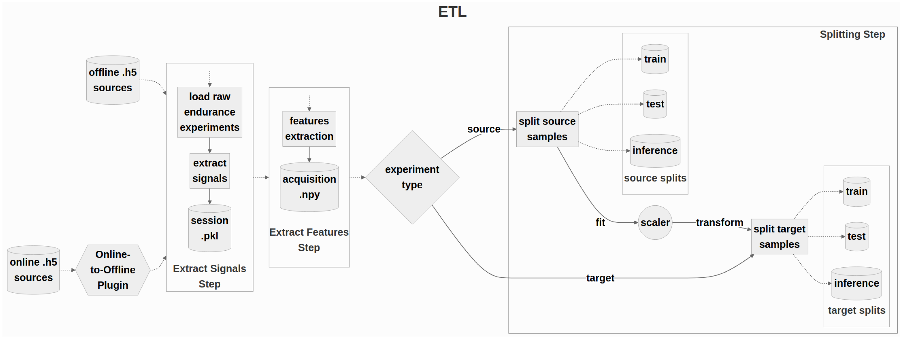
Figure 2.
Anomaly Detection Setup with Multiple-Variational Autoencoders.
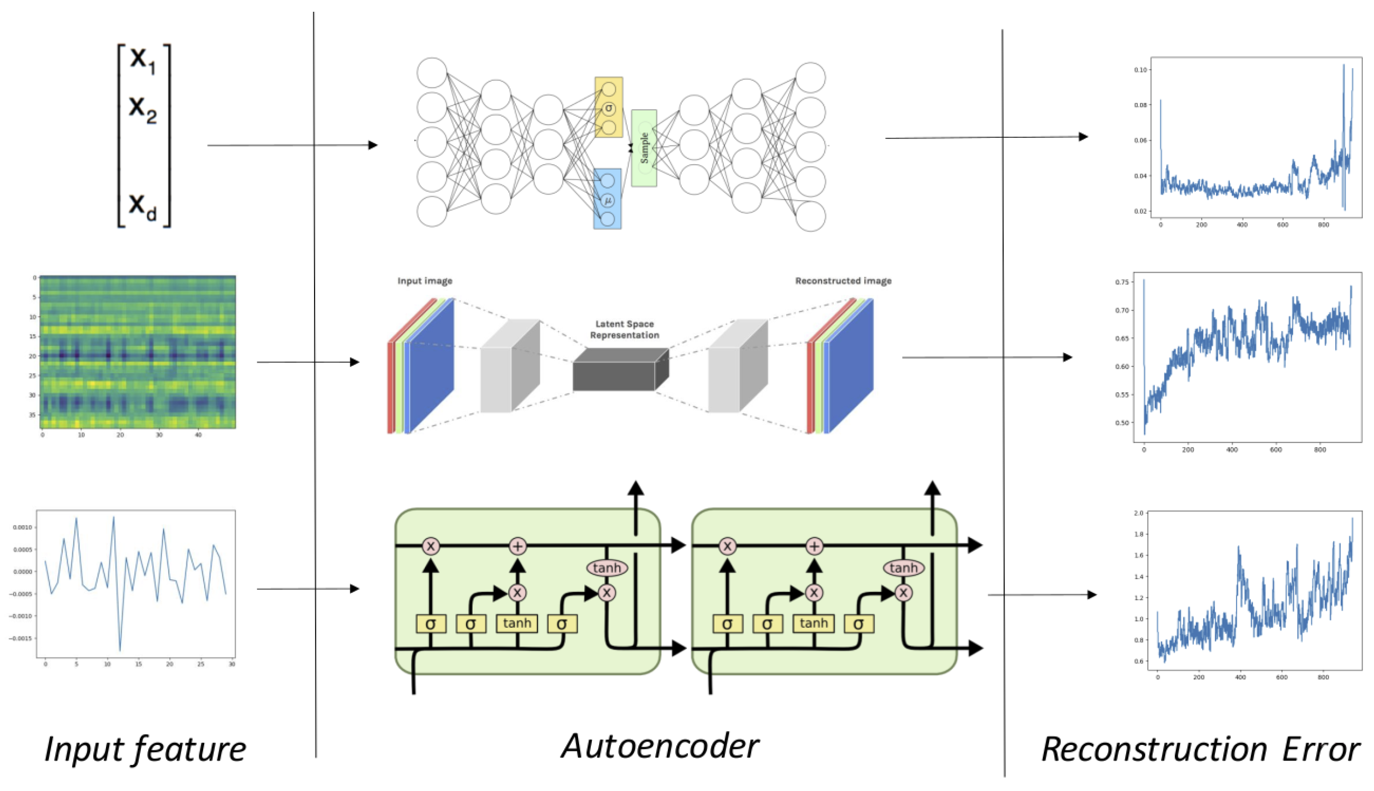
Figure 3.
Workflow of the predictive models with domain adaptation.
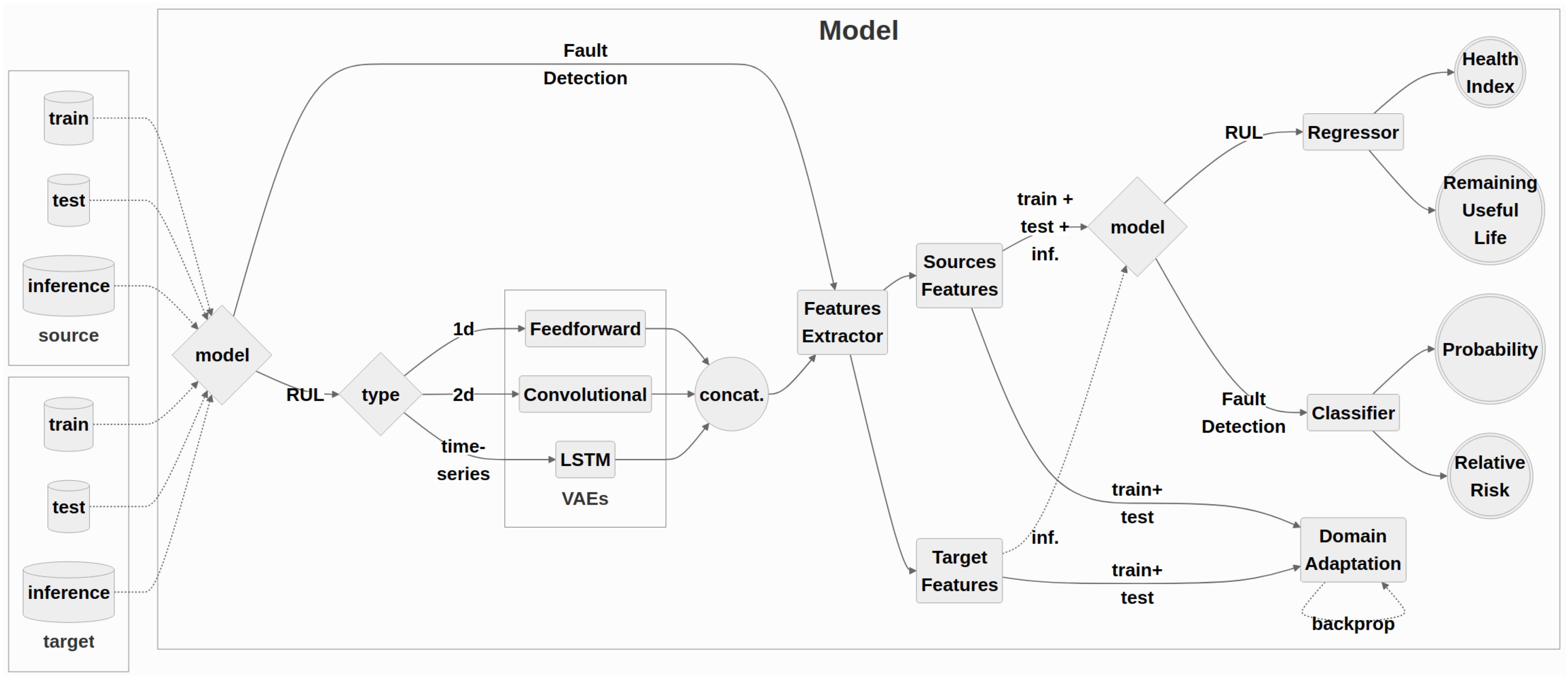
Figure 4.
Example of Diagnosis predictions on a real-world experiment.
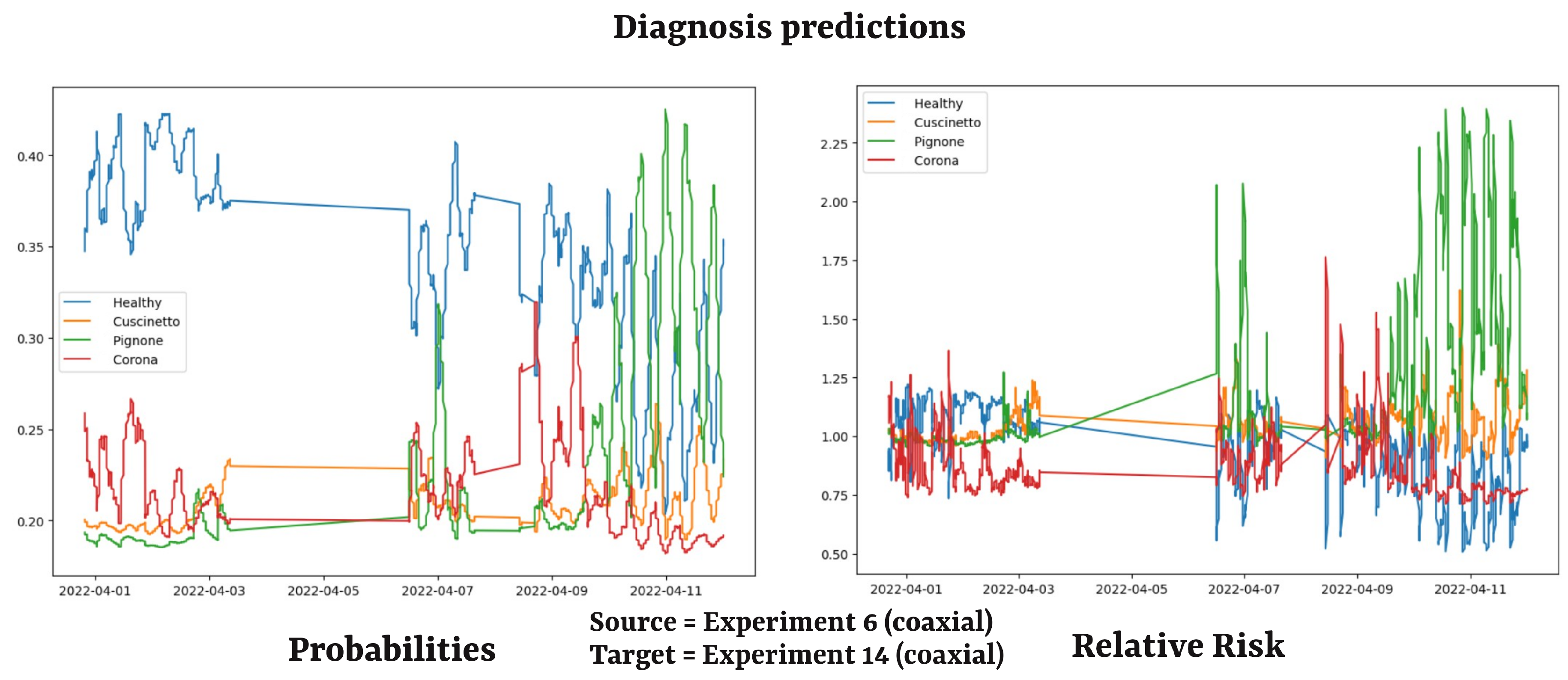
Figure 5.
Example of prognostic prediction in a real-time experiment.
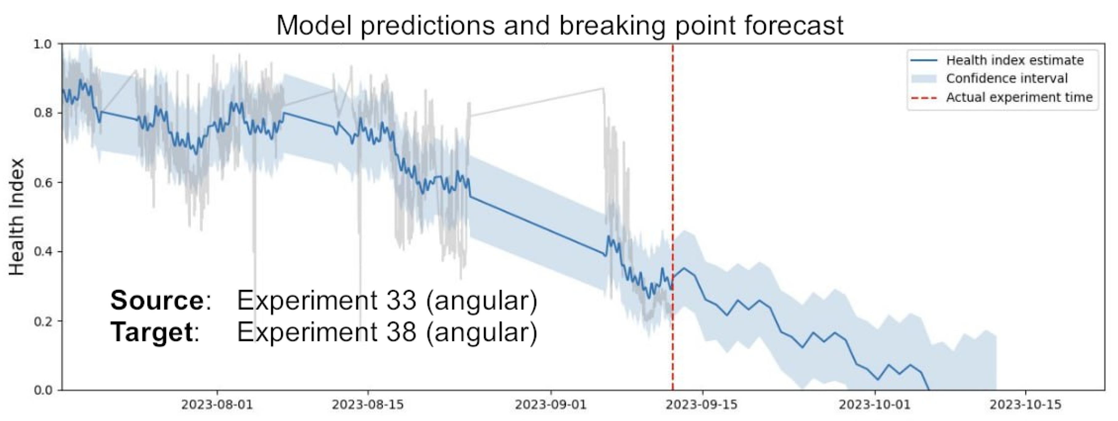
Disclaimer/Publisher’s Note: The statements, opinions and data contained in all publications are solely those of the individual author(s) and contributor(s) and not of MDPI and/or the editor(s). MDPI and/or the editor(s) disclaim responsibility for any injury to people or property resulting from any ideas, methods, instructions or products referred to in the content. |
© 2024 by the authors. Licensee MDPI, Basel, Switzerland. This article is an open access article distributed under the terms and conditions of the Creative Commons Attribution (CC BY) license (http://creativecommons.org/licenses/by/4.0/).
Copyright: This open access article is published under a Creative Commons CC BY 4.0 license, which permit the free download, distribution, and reuse, provided that the author and preprint are cited in any reuse.


