
Submitted:
21 July 2025
Posted:
23 July 2025
You are already at the latest version
Abstract
Traditionally, duct sizing in ventilation systems is based on balancing pressure losses across all branches, with fan selection performed subsequently. However, this sequential approach is inadequate for systems with distributed fans in the central duct network, where pressure losses can vary significantly. Consequently, when designing the system topology, fan placement and duct sizing must be considered together. Recent research has demonstrated that discrete optimisation methods can account for multiple load cases and produce ventilation layouts that are both cost- and energy-efficient. However, existing approaches usually concentrate on component placement and assume that duct sizing has already been finalised. While this is sufficient for later design stages, it is unsuitable for the early stages of planning, when numerous system configurations must be evaluated quickly. In this work, we present a novel methodology that simultaneously optimises duct sizing, fan placement, and volume flow controller configuration to minimise life-cycle costs. To achieve this, we exploit the structure of the problem and formulate a Mixed-Integer Linear Program (MILP), which, unlike existing non-linear models, significantly reduces computation time while introducing only minor approximation errors. The resulting model enables fast and robust early-stage planning, providing optimal solutions in a matter of seconds to minutes as demonstrated by a case study.
Keywords:
ventilation system design
; system optimization
; fan placement optimization
1. Introduction
With increasing pressure to reduce energy consumption and meet climate targets, the energy efficiency of ventilation systems is gaining importance. In the European Union, fans account for approximately 12.3% of the total electrical energy demand [1]. Mechanical ventilation systems have the potential to reduce overall energy consumption. This reduction is achievable when these systems incorporate heat recovery mechanisms and are paired with highly insulated building designs. However, this energy saving potential depends on the fans themselves having a low energy demand [2].
This raises the question of how to reduce fan power demand. The electrical power demand of a system with multiple fans is the sum of the individual fan’s power demands , which can be calculated by
with the fan’s pressure increase , volume flow q and efficiency . The total electrical power demand of a system thus can be reduced by (i) lowering the volume flows, (ii) reducing the pressure losses in the system or (iii) increasing efficiency.
The volume flows (i) can be reduced to the actual demand, with variable volume flow systems, this is state-of-the-art and thus assumed given. The pressure losses (ii) depend on the system topology: In a central system, central fans must overcome the highest pressure loss across all branches. Distributed systems, in contrast, can reduce this requirement by integrating additional fans into high-loss branches. Research from the University of Kassel has demonstrated the potential and practicality of this approach [3,4], and optimisation-based methods have further refined distributed fan system design [5,6]. Wider ducts can also reduce pressure losses by lowering airflow resistance. Finally, improving efficiency (iii) involves ensuring all components — fans and volume flow controllers (VFCs) —operate within efficient regimes.
Considering all three factors simultaneously is challenging for human planners, which is why heuristic methods are commonly used instead. In the literature, duct sizing is often approached by balancing pressure losses across all branches [7]. However, this approach does not incorporate the trade-off between electrical energy costs and investment costs. Moreover, it fails in the presence of distributed fans. A common approach sizes ducts by balancing pressure losses across branches [7], but this ignores investment vs. operational cost trade-offs and fails when distributed fans are used. Some recent methods optimise component selection and operation within fixed duct layouts [5,6] with detailed fan characteristics, including acoustic considerations [6,8]. However, they do not address early-stage duct layout and dimensioning.
The first planning phase — preplanning — defines the ventilation system’s basic layout. At this stage, the duct network is roughly established, and the number and placement of components such as fans and VFCs are determined. Due to coordination with other building trades, the layout is typically fixed externally, and planning is divided into two tasks: duct sizing and component placement.
In this paper, we propose a novel optimisation-based approach for early-stage ventilation planning. Specifically, we address the joint optimisation of duct sizing and fan placement - including the use of distributed fans. The model captures fundamental trade-offs, such as whether to increase duct cross-sections to reduce pressure losses, or to install additional fans in high-loss branches to lower energy consumption.
To formulate this problem, we use tools from mathematical optimisation, and more precisely, from discrete optimisation. Discrete optimisation allows us to model binary decisions, such as whether a fan or volume flow controller (VFC) is installed, in combination with continuous decisions such as duct dimensions or fan speeds. This approach is particularly well-suited for early design stages, where many components are either present or absent and must be selected from a catalogue of options.
Furthermore, to reflect realistic operating conditions, we model multiple load cases and define a two-stage stochastic optimisation problem. The first stage captures investment decisions, while the second stage evaluates operational performance under varying demand. To ensure computational tractability, we linearise both fan characteristics and pressure loss equations. This enables the solution of large instances within seconds, making the method highly suitable for practical use in preplanning.
By explicitly formulating the planning task as a discrete optimisation problem, we bridge the gap between coarse high-level models and detailed component-level planning. The proposed model enables early-stage planners to systematically explore design trade-offs and generate energy-efficient, cost-effective system layouts - even under uncertainty.
2. Methods
The following section introduces the system model, the fan model, and the duct model in detail.
2.1. System Model
The supply and exhaust air systems are modelled separately, and the ventilation system can be represented as a mathematical tree-like graph , where the nodes are and the edges are . The ventilation system model is formulated as a Mixed-Integer Linear Program (MILP). This model includes the objective function, the mathematical graph representation of the system, the component models (see following subsections), the load cases , topology constraints, and conservation equations. The fans, VFCs and ducts are defined on the edges .
The mathematical optimisation problem is structured into two stages:
- Determining a cost-effective purchase decision for the components.
- Operating a subset of the purchased components for each load case within the specified load profile, ensuring that the system meets the demand while maximising efficiency.
The load cases differ in volume flow demand for each room. This formulation results in a 2-stage stochastic MILP. The system model is not given in detail, refer to [6] section 2.3 for the model.
The objective of the optimisation is to minimise the life-cycle costs, consisting of:
(i) Investment costs, including costs for fans (fan-type dependent : ), VFCs (), and ducts (, see Equation (10)) and
(ii) Operating costs, determined by the load case frequency , electrical energy cost in , the ventilation system’s entire operation time in hours and the energy consumption of the fans .
The investment costs are calculated according to the annuity method described in [9]. With these costs, the objective function can be expressed as:
For improved clarity, this paper uses capital letters to denote parameters of the optimisation model and lowercase letters to represent variables.
Fan, VFC, and pressure loss models for ducts and fittings complete the system model. The VFCs are modelled to allow a variable pressure loss when purchased. The remaining models are presented in the following.
2.2. Fan Station Model
Each fan is described by its rotational speed n, volume flow q, pressure increase and its electrical energy consumption . These relationships are defined by manufacturer data in the form of two curves: one describing pressure as a function of flow and speed , and one describing power consumption as a function of the same :
where () and () are fan-specific constants derived from fitting manufacturer data.
To operate multiple fans in parallel, their pressure increase is set equal and only their volume flow may be different. As shown by Groß et al., in case of identical parallel fans, maximum efficiency is achieved when the fans operate identically [10]. This is modelled with additional constraints. Fans can be purchased at the cost , and only a purchased fan can be activated in the load cases.
The fan characteristic curves are non-linear and non-convex, which makes them difficult to include directly in an optimisation problem. To ensure fast solving times, the curves are simplified using a linear approximation technique. Common techniques to handle the complexity are linearisation approaches adding binary (yes/no) variables (i.e., piecewise linear approximations). These however still have extensive solving times, compare [11]. Another approach from the field of discrete optimisation is to approximate the fan curves using linear approximations without introducing binary variables (i.e., outer polyhedral approximation).
The key is to express the fan’s electrical power demand as a function of flow and pressure, and to approximate this function from below using linear expressions. This results in conservative estimates, ensuring that energy demand is never underestimated. In the following we outline the core procedure for constructing these linear fan models:
- Fan power consumption is expressed as a function of flow and pressure , using the fan pressure curve Equation (4).
- For multiple parallel fans, the total electrical power consumption is split into hydraulic power, , and the residual losses , such that . Since the total flow rate Q is known in advance (unlike the individual flows), the hyraulic term is linear. Moreover, the loss function exhibits a smaller locally non-convex region than the full fan curve.
- The power loss function is linearised for each fan by constructing a set of linear inequalities - lower bounds at selected operating points (i.e., outer polyhedral approximation). Since the optimisation minimises electrical power, the solution will lie on one of these lower bounding constraints.
- Because the fan speed is no longer a decision variable, it must be constrained indirectly to stay within feasible bounds. This is achieved via additional linear inequalities that ensure the estimated electrical power does not exceed the value at 100 % fan speed.
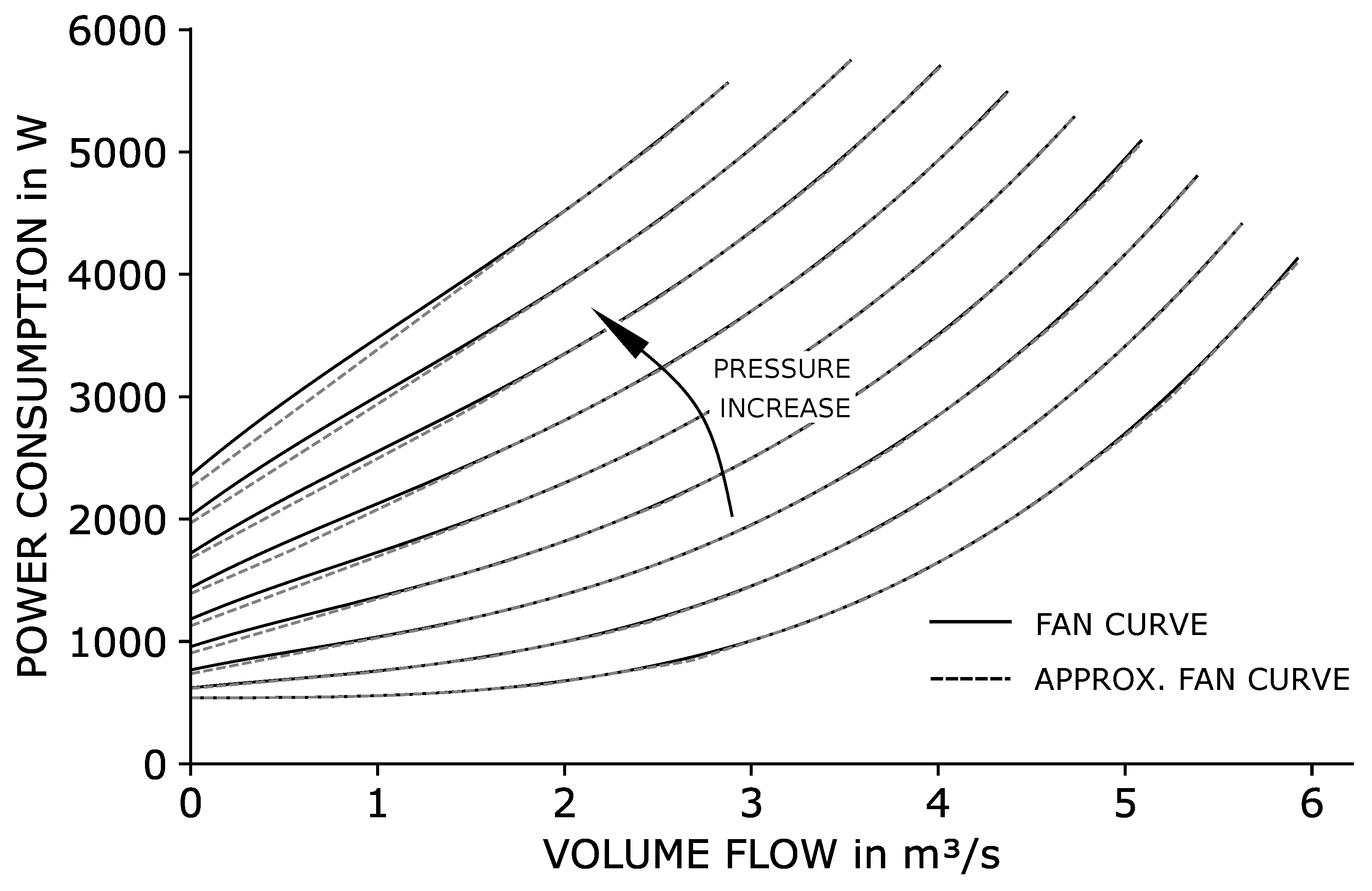
This linearisation enables highly efficient computation. However, in certain non-linear regions of the power loss model, the approximation visibly deviates from the true fan behaviour (see fig:fanapproximation).
Because the model underestimates power losses by definition, the computed power consumption represents a lower bound: no real system can perform better than this. To assess the actual system performance, we can recalculate the exact power consumption of the optimised solution by evaluating the exact fan model at the resulting pressure and flow values. This yields an upper bound. As a result, the exact life-cycle cost of the system lies within a bounded range between the estimated and the recalculated exact values. This solution bounding approach allows engineers to evaluate how close the optimisation result is to the true optimum – while ensuring fast computation.
Figure 1.
Approximation of an example fan curve: The dashed lines represent approximations of the solid lines representing non-linear fan curves. At low volume flows and high pressure losses, the electric power is visibly underestimated, while at high volume flows, the approximation error is minimal.
2.3. Pressure Losses
The pressure losses are present on every edge of the graph that represents the duct network or auxiliary components other than fan stations. As the duct topology is fixed, each duct’s length L as well as the volume flow Q through the ducts and auxiliary components are known beforehand. Given the volume flows, the auxiliary components’ pressure losses are calculated a priori and are thus not part of the optimisation. Concerning the ducting, the design variables are only the width w and the height h. The pressure loss is described by
with density and resistance coefficient .
For duct friction, can be calculated using the Darcy-Weisbach equation [12]:
with being the friction factor dependent on the relative roughness and the Reynolds number . For simplicity is assumed to be constant. is the hydraulic diameter of a rectangular cross-section. Plugging Equation (7) into Equation (6) and reformulating, one obtains
For fittings, the pressure loss depends on geometrical and/or flow factors. The fitting-dependent resistance coefficient is calculated according to VDI standard 3803 part 6 [13]. For most fittings it is feasible to approximate a fixed value that can be calculate a-priori. For a branch, the pressure loss strongly depends on the ratio of velocities in the branches. To avoid excessive pressure losses in branches, configurations with very small velocity ratios are excluded from the optimisation.
Since the above equations are highly non-linear in width and height, they are linearised to maintain solver efficiency. For the pressure loss model, it can be shown, that the general pressure loss formula Equation (6) as well as the duct friction formula Equation (9) are convex functions w.r.t. width w and height h. A proof is provided in Appendix A.1, but is not required for understanding the method. Since the optimisation aims to minimise pressure losses for given w and h, the non-linear expressions are again approximated from below using linear constraints (i.e., polyhedral outer approximation).
The investment cost of ducts is proportional to their surface area and can be expressed as:
with being the duct costs in .
3. Case Study
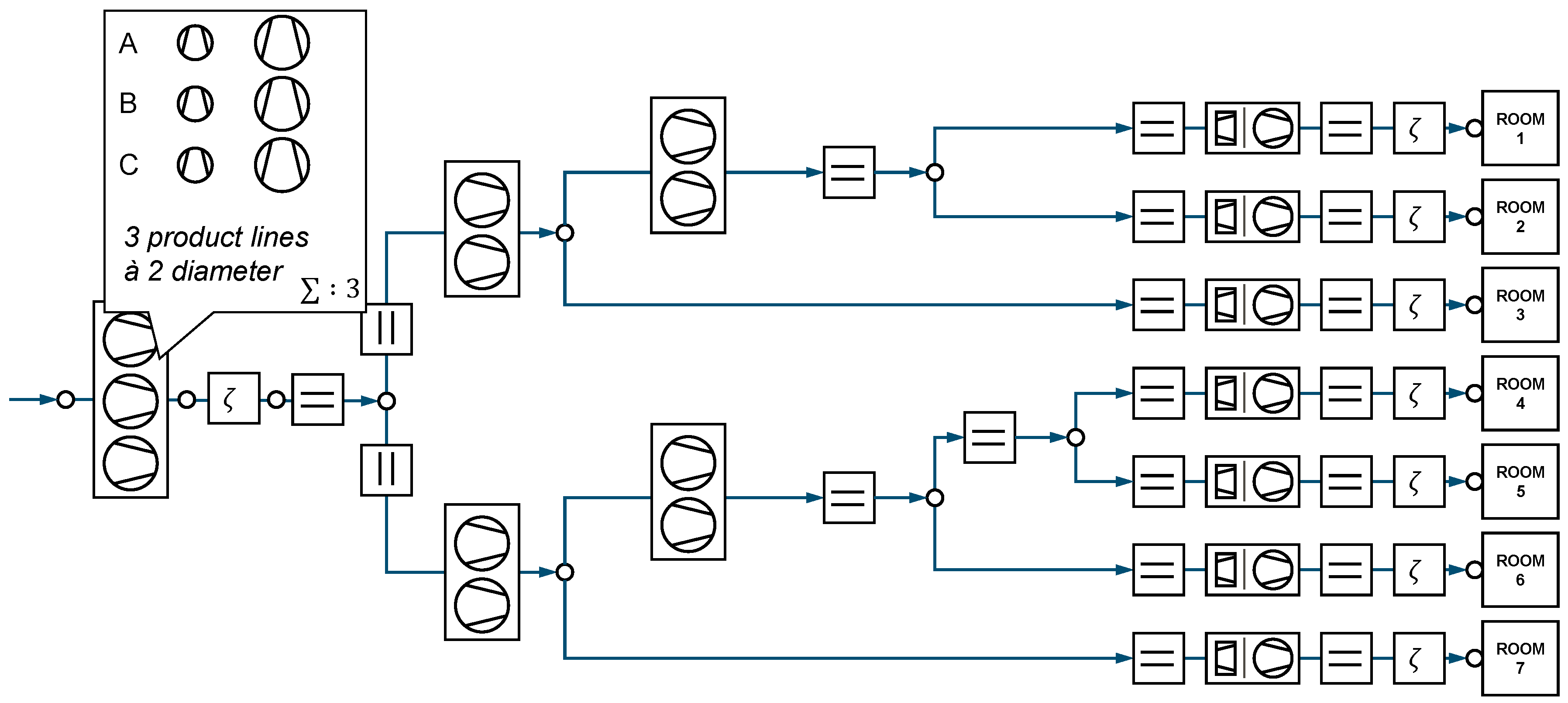
In this case study, the same building and load cases as in Breuer [6] are optimised, see fig:problem. Only the supply air system is optimised. The system is planned to operate for 12 years. The duct network layout is predefined; however, the width w and height h of each section remain to be determined as part of the optimisation process. The dimensions of the ducts range between and , except for the central duct, where the maximum dimension is .
The central fan station can accommodate up to three fans, selected from two product lines with two different diameters. Each individual fan type can be installed up to three times. Additionally, upstream of each room and each branch up to three fans – chosen from the same set of fans as those used centrally – and/or a VFC can be installed. The case where both, fans and a VFC, are purchased would result in a parallel arrangement where either one or the other component is active.
Figure 2.
The case study building’s ventilation system supplies outdoor air to seven rooms. The blocks represent system components: in addition to the fan and VFC blocks, there is a -value block with a prescribed -value. The blocks with two horizontal parallel lines represent duct sections that require dimensioning. When distributed fans are present, the branches require shut-off dampers, which are not shown in this diagram.
4. Results
The mathematical models are implemented in Python using the PYOMO [14] modelling language and solved using Gurobi 12.0.1 [15]. Gurobi employs a branch-and-bound algorithm to solve the problem. The computations were carried out on a Ubuntu Workstation with Ubuntu 24.04 operating system, 80 GB of RAM, and two AMD EPYC 7313 32-core processors and a maximum clock speed of 3.7 GHz.
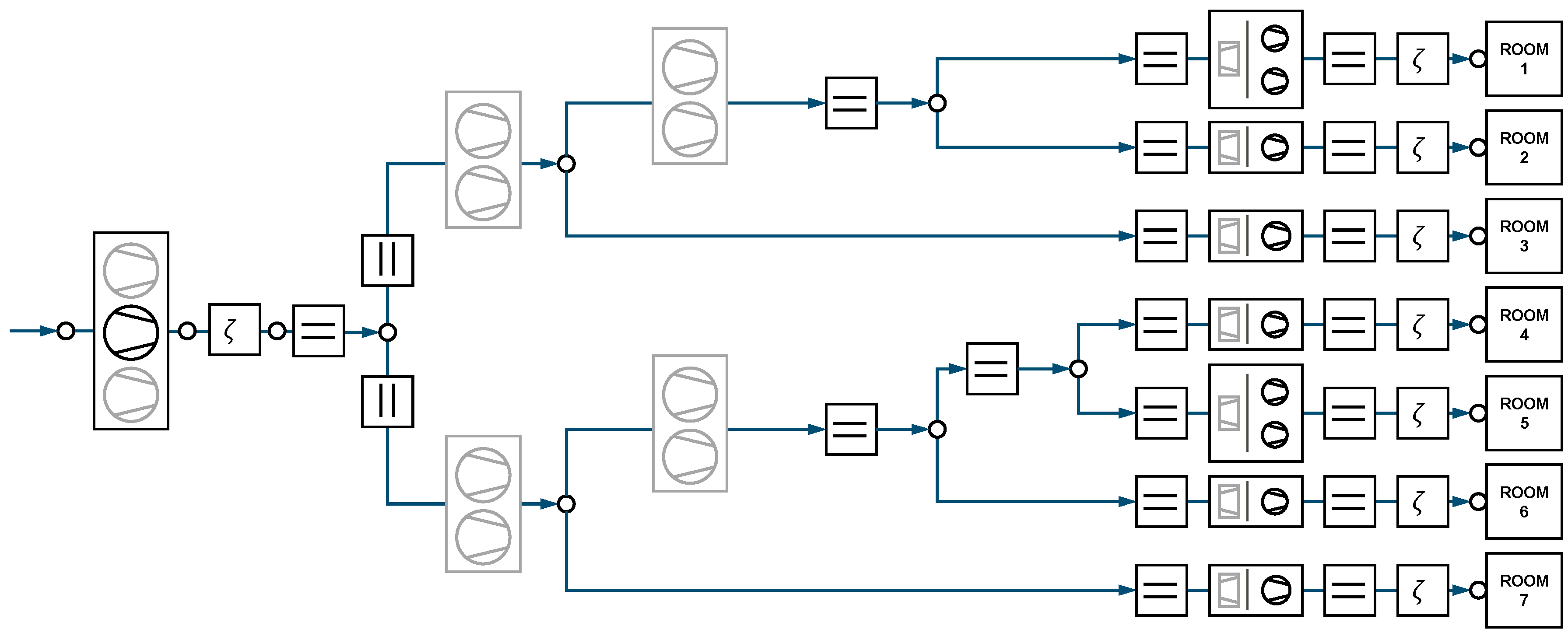
The resulting ventilation system is shown in fig:solution. A single fan is purchased centrally, no fan is purchased in front of a branch and in front of each room one or two fans but no VFCs are purchased – the optimal topology is distributed. In comparison to the optimal central solution (which is not shown here), the system has decreased life-cycle costs. Counter-intuitively, this does not stem from decreased energy costs but from the fact that the cheapest fans are cheaper than the cheapest VFCs.
Figure 3.
A distributed system is the optimal configuration for the case study building. A single fan is purchased centrally while in front of every room one or two fans are purchased.
Figure 3.
A distributed system is the optimal configuration for the case study building. A single fan is purchased centrally while in front of every room one or two fans are purchased.
The life-cycle costs of the system are 49 255 €. The cost distribution is given in fig:costdistribution. The largest cost factor, at 41 %, is the duct investment costs, followed by the fan electric energy costs with . The fan investment cost is just below that.
Figure 4.
Cost distribution of optimal solution. Duct investment costs are the biggest cost factor.
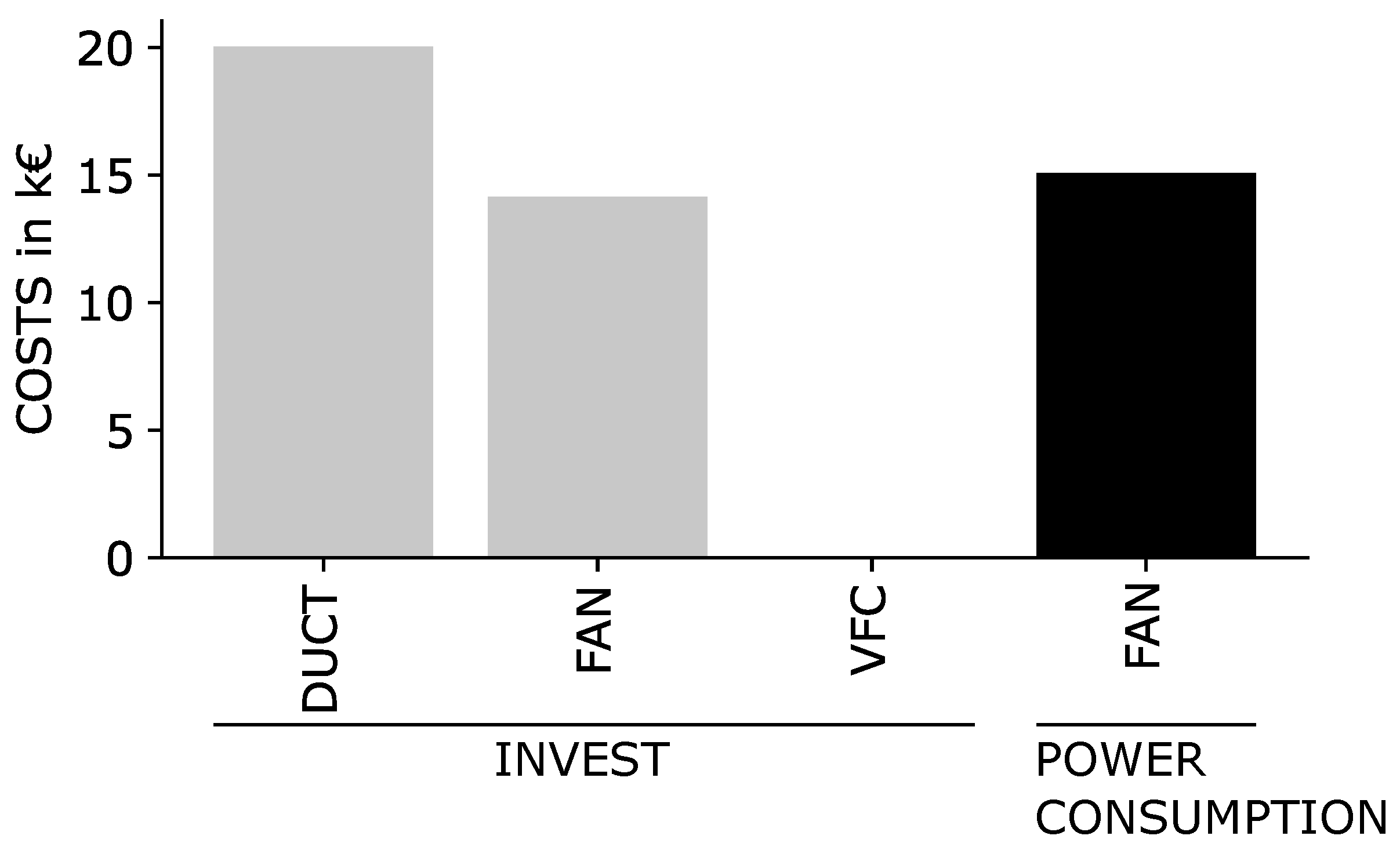
Figure 5.
Comparisons of exact values and those approximated using outer polyhedral approximation. The line with unit slope represents exact similarity between exact and approximated values.
Figure 5.
Comparisons of exact values and those approximated using outer polyhedral approximation. The line with unit slope represents exact similarity between exact and approximated values.
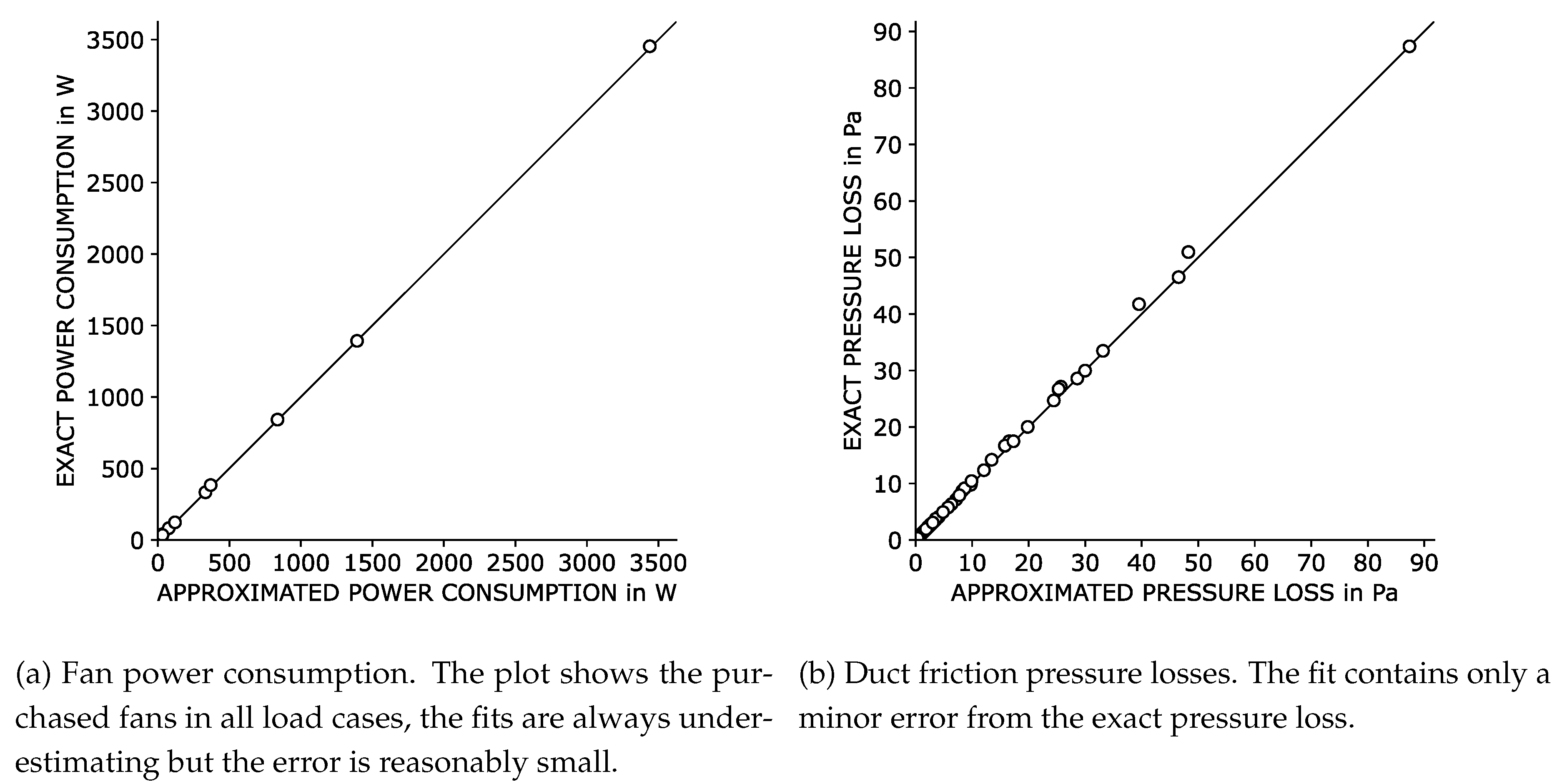
As multiple approximations are employed, it is important to evaluate the approximation errors. Using the known operating points, the fan’s exact electrical power consumption can be calculated. Similarly, with the known duct dimensions, the exact friction pressure loss per duct can also be determined. The approximated values are then compared to the exact values, as shown in fig:approximationerrors. Overall, the approximation demonstrates good agreement with the exact values. Using the solution bounding approach, it is made sure that any optimisation performed using exact fan characteristic curves will yield results that lie between the approximated and the exact problem. In other words, optimising the topology with exact fan characteristic curves could, at best, achieve up to 1.4 % lower electrical power consumption compared to the current approximated topology.
5. Discussion and Conclusions
This paper introduces a novel methodology that enables a systematic trade-off between larger duct dimensions and distributed fans. By utilising mathematical optimisation, the approach provides valuable insights into the optimal design and behaviour of ventilation systems, balancing investment costs and operational efficiency.
The results of the presented case study demonstrate the capability of the methodology to solve complex preplanning tasks within seconds. This efficiency stems from the linear nature of the problem formulation, which ensures very low computational times. For comparison, solving the same problem using the original non-linear fan models (Equations (4) and (5)) takes multiple hours, whereas the linearised model solves within 2.5 min.
The results further show that the approximated fan power and pressure losses align closely with exact values. The observed deviation of up to 1.4 % from the exact power consumption is a reasonably small error given the significant reduction in solving times. This trade-off between accuracy and computational efficiency makes the methodology particularly suitable for the preplanning stage. In the preplanning stage, planners typically try many different topologies. Using the method shown in this paper, the planners can optimise different duct network topologies within seconds and compare their results. The solution bounding approach even allows statements of the non-approximated system’s optimal life-cycle costs.
In the case study, duct width and height were treated as independent parameters, allowing them to vary within identical ranges. However, this approach may not fully align with practical applications, as the optimisation naturally leads to symmetric duct dimensions for maximum efficiency. In real-world planning, dimensions are often influenced by constraints imposed by other building trades, particularly limitations on duct height. Such constraints can be directly incorporated into the optimisation process by setting upper limits on duct height or allowing only specific width-to-height ratios. Additionally, due to the iterative nature of the planning process and interactions with other trades, spatial limitations frequently arise. For example, it is often not feasible to increase duct dimensions beyond a certain height simply because there is not enough available space.
The findings of this case study should not be generalised. A larger-scale investigation involving multiple buildings with more complex ventilation systems is needed to better identify scenarios where distributed fans provide significant value. Yet, first results on a larger building with more distributed fans and more fan product lines show that the methodology’s computational efficiency scales well and solves within a few minutes. In contrast, solving the non-linear formulation takes multiple days. The accuracy of the larger building’s solution is even better than in this case study.
Further research could also include integrating heat demands and respective components into the optimisation framework. This extension would enable an even more comprehensive evaluation of system performance and energy efficiency, further broadening the applicability of the methodology.
Author Contributions
Conceptualization, Julius Breuer; Data curation, Julius Breuer; Funding acquisition, Peter Pelz; Methodology, Julius Breuer; Project administration, Julius Breuer and Peter Pelz; Software, Julius Breuer; Supervision, Peter Pelz; Validation, Julius Breuer; Visualization, Julius Breuer; Writing – original draft, Julius Breuer; Writing – review & editing, Julius Breuer.
Funding
The presented results were obtained within the research project “Algorithmic System Planning of Air Handling Units”, Project No. 22289 N/1, funded by the program for promoting the Industrial Collective Research (IGF) of the German Ministry of Economic Affairs and Climate Action (BMWK), approved by the Deutsches Zentrum für Luft- und Raumfahrt (DLR). We want to thank all the participants of the working group for the constructive collaboration.
Data Availability Statement
Not applicable.
Conflicts of Interest
“The authors declare no conflicts of interest.”
Abbreviations
The following abbreviations are used in this manuscript:
| VFC | Volume flow controller |
| MILP | Mixed-Integer Linear Program |
Appendix A.
Appendix A.1. CONVEXITY
To show that the general pressure loss formula Equation (6) as well as the duct friction formula Equation (9) are convex functions w.r.t. width w and height h, we show that their curvature is always positive. As these functions are multivariate, their Hessian must thus be positive semi-definite.
To show this, first the general pressure loss formula Equation (6) is simplified by removing its constant factors.
Now, we calculate the Hessian
and thus, the principal minors are non-negative:
Similarly, the principal minors of the duct friction Equation (9) are also non-negative and thus the duct friction is convex.
References
- European Commission. Commission Regulation (EU) No 327/2011 of 30 March 2011 implementing Directive 2009/125/EC with regard to ecodesign requirements for fans driven by motors with an electric input power between 125 W and 500 kW. http://data.europa.eu/eli/reg/2011/327/oj, 2011. EU Regulation, Official Journal L 90, pp. 8–21, 6 April 2011.
- Federal Ministry for Economic Affairs and Energy. Energy Efficiency Strategy for Buildings: Methods for Achieving a Virtually Climate-Neutral Building Stock. Government report, BMWi, Berlin, Germany, 2015.
- Alsen, N.; Klimmt, T.; Knissel, J.; Giesen, M. Einsatz dezentraler Ventilatoren zur Luftförderung in zentralen RLT-Anlagen insbesondere bei Nicht-Wohngebäuden. Final report, Kassel University, 2018.
- Knissel, J.; Giesen, M.; Klimmt, T. Planungsleitfaden Semizentrale Lüftung – Dezentrale Ventilatoren in zentralen RLT-Anlagen. Final report, University of Kassel, 2018.
- Müller, T.M.; Sachs, M.; Breuer, J.H.; Pelz, P.F. Planning of distributed ventilation systems for energy-efficient buildings by discrete optimisation. Journal of Building Engineering 2023, 68, 106205. [Google Scholar] [CrossRef]
- Breuer, J.H.; Pelz, P.F. Algorithmic planning of ventilation systems: Optimising for life-cycle costs and acoustic comfort. Journal of Building Engineering 2025, 99, 111547. [Google Scholar] [CrossRef]
- Kabbara, Z.; Jorens, S.; Ahmadian, E.; Verhaert, I. Improving HVAC ductwork designs while considering fittings at an early stage. Building and Environment 2023, 237, 110272. [Google Scholar] [CrossRef]
- Breuer, J.H.P.; Pelz, P.F. Efficient and Quiet: Optimisation of Ventilation Systems by coupling Airflow with Acoustics in a Multipole Approach. In Operations Research Proceedings 2023: Selected Papers of the Annual International Conference of the German Operations Research Society (GOR 2023); Lecture Notes in Operations Research, Springer, Cham: Cham, Switzerland, 2025; pp. 1–7. [Google Scholar]
- Verein Deutscher Ingenieure (VDI). VDI 2067 Blatt 1: Economic efficiency of building installations – Fundamentals and cost calculation; VDI-Verlag: Düsseldorf, Germany, 2012. [Google Scholar]
- Groß, T.F.; Pöttgen, P.F.; Pelz, P.F. Analytical Approach for the Optimal Operation of Pumps in Booster Systems. Journal of Water Resources Planning and Management 2017, 143, 04017029. [Google Scholar] [CrossRef]
- Müller, T.M.; Leise, P.; Lorenz, I.S.; Altherr, L.C.; Pelz, P.F. Optimization and validation of pumping system design and operation for water supply in high-rise buildings. Optimization and Engineering 2021, 22, 643–686. [Google Scholar] [CrossRef]
- Idelchik, I.E.; Steinberg, M.O.; Martynenko, O.G. Handbook of hydraulic resistance; Vol. 2, Hemisphere publishing corporation New York, 1986.
- Verein Deutscher Ingenieure (VDI). VDI 3803 Blatt 6: Luftleitsysteme – Druckverluste und wärmetechnische Berechnungen; VDI-Verlag: Düsseldorf, Germany, 2023. [Google Scholar]
- Hart, W.E.; Watson, J.P.; Woodruff, D.L. Pyomo: Modeling and solving mathematical programs in Python. Mathematical Programming Computation 2011, 3, 219–260. [Google Scholar] [CrossRef]
- Gurobi Optimization, LLC. Gurobi Optimizer Reference Manual, 2023.
Disclaimer/Publisher’s Note: The statements, opinions and data contained in all publications are solely those of the individual author(s) and contributor(s) and not of MDPI and/or the editor(s). MDPI and/or the editor(s) disclaim responsibility for any injury to people or property resulting from any ideas, methods, instructions or products referred to in the content. |
© 2025 by the authors. Licensee MDPI, Basel, Switzerland. This article is an open access article distributed under the terms and conditions of the Creative Commons Attribution (CC BY) license (http://creativecommons.org/licenses/by/4.0/).
Copyright: This open access article is published under a Creative Commons CC BY 4.0 license, which permit the free download, distribution, and reuse, provided that the author and preprint are cited in any reuse.


