
Submitted:
21 July 2025
Posted:
22 July 2025
You are already at the latest version
Abstract
In this study, a hybrid sensor-based electronic nose circuit was developed using eight metal-oxide semiconductors and 14 quartz crystal microbalance gas sensors. The study included 100 participants: 60 individuals diagnosed with lung cancer, 20 healthy nonsmokers, and 20 healthy smokers. A total of 338 experiments were performed using the breath samples throughout the study. In the classification phase of the obtained data, in addition to traditional classification algorithms, such as decision trees, support vector machines, k-nearest neighbors, and random forests, the fuzzy logic method supported by the optimization algorithm was also used. While the data were classified using the fuzzy logic method, the parameters of the membership functions were optimized using a nature-inspired optimization algorithm. In addition, principal component analysis and linear discriminant analysis were used to determine the effects of dimension-reduction algorithms. As a result of all the operations performed, the highest classification accuracy of 94.58% was achieved using traditional classification algorithms, whereas the data were classified with 97.93% accuracy using the fuzzy logic method optimized with optimization algorithms inspired by nature.
Keywords:
breath analysis
; hybrid sensor based electronic nose
; lung cancer detection
; data classification and fuzzy logic algorithm
; nature inspired optimization algorithms
1. Introduction
Motivation: Lung cancer (LC) has the highest mortality rate of all cancers worldwide. According to the World Health Organization (WHO) data, the global mortality rate of LC surpasses that of combined kidney, colorectal, and prostate cancers [1,2]. Although LC ranks second after bowel cancer in terms of the number of diagnosed cancers, it stands out as a form of cancer associated with the highest fatality rate. Globally, there were 10 million fatalities attributed to cancer, and 19.3 million new cancer cases were reported, according to the GLOBOCAN 2020 data. The two most common cancers in terms of incidence and mortality are LC and breast cancer, respectively. Figure 1 illustrates the incidence of new cancer cases and cancer-related fatalities in 2020, as reported by GLOBOCAN [3].
Studies have shown that while the five-year survival rate of individuals diagnosed with LC in the early stages can reach up to 90%, this rate drops below 10% in individuals whose disease is detected in the advanced stages [4]. Changes in the 5-year survival rates according to the stage at which LC is detected are shown in Figure 2 [5]. Various medical methods have been employed to examine individuals in the high-risk category for the early identification of LC. These approaches typically encompass a combination of saliva cytology [6,7], analysis of circulating tumor biomarkers [8,9], examination of blood protein structure [10,11], chest tomography [12,13], nuclear magnetic resonance [14], chest radiography [15], and low-dose computed tomography [16], among others. Because these methods exhibit restricted diagnostic capabilities when employed for an extended period, ongoing research is aimed at enhancing their performance. The limited success of imaging techniques for early stage LC detection and mortality reduction has prompted researchers to focus on breath analysis in this field.
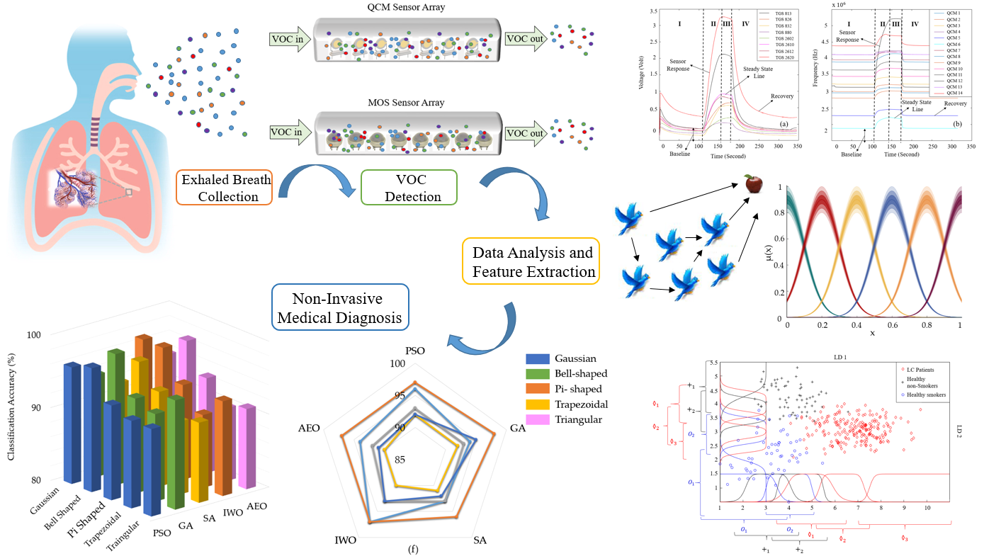
Proposed approach: Studies in the field of breath analysis aims to identify and measure volatile organic molecules (VOCs), which may be disease markers, in the breath.
Any imbalance in the functioning of the organs in the body causes the amount of VOCs detected in the breath to change. When studies on breath analysis were examined, it was determined that in cases of febrile illness and sepsis, the pentane concentration in the breath was higher than that in healthy individuals [17]. Individuals with diabetes, a widespread global ailment, exhibit elevated levels of acetone and methyl nitrate in their exhaled breath [18,19]. Ammonia and di/trimethylamine are nitrogen-containing compounds present in the breath, and these volatile organic compounds are notably detected in the breath of individuals with kidney disease [20,21]. In addition, many studies have examined the VOCs in the breath associated with LC diseases. In a study examining LC, which is the subject of this study, Peng et al. examined VOCs found in the breath of patients with cancer using gas chromatography-mass spectrometry (GC-MS) performed on four different types of cancer: LC, bowel cancer, breast cancer, and prostate cancer. As a result of the study, they identified 80% non-overlapping VOCs in the breaths of patients and healthy people. The identified VOCs were quantified as 33, 54, 34, and 36 for lung cancer,breast cancer, 34 for bowel cancer, and 36 for prostate cancer, respectively [22]. In a study carried out by Poli and his colleagues, they examined the aldehyde levels in the exhaled breath of individuals with LC. In their studies, researchers determined that propanal, butanal, pentanal, hexanal, heptanal, octanal, and nonanal aldehyde levels were different in the breath samples of the collection groups [23]. Jia et al. examined 25 studies in the literature in their review article on the breath content of individuals with LC. Biomarkers identified in a minimum of four studies were filtered and prioritized based on their frequency of occurrence. These VOCs were identified as toluene, propanol, isoprene, pentanol, acetone, hexane, ethyl benzene, 2-butanol, Benzene, heptane, propanal, pentanal, ethanol, butanol, and benzene [24].
GC-MS is mostly utilized in these studies to ascertain breath content. In addition to these methods, ion flow tube mass spectrometry, laser absorption spectrometry, and infrared spectroscopy have been extensively utilized to identify VOCs in breath. However, these devices require methods are expensive, and the tests are performed for a long time. Moreover, the preconcentration of breath samples is essential for enhancing the efficiency of VOC detection using these methods.
Hardware and data analysis approaches: compared with the above methods, electronic noses (e-noses) are cheaper and, easier to install and use. In addition, no concentration process was required before the experiments. Target gases can be detected and distinguished with high accuracy using the appropriate sensors. The e-nose is an instrument inspired by the biological olfactory system of living organisms. Owing to its structure, which has both a chemical detection system and a data processing system, it can detect many simple and complex odors. These devices primarily comprise three components: a sensing unit, an electronic module, and a pattern-recognition component. An illustrated comparison of the e-nose and mammalian olfactory systems is shown in Figure 3 [25]. Numerous studies have utilized e-nose technology for breath analysis to detect lung cancer. Nakleh et al. conducted experiments using an e-nose with breath samples collected from patients with LC (n=45), patients with different cancer types (n=357), and controls (n=411). They used Au and a single-walled carbon nanotube-based e-nose and classified the data with a success rate of 85% [26]. Binson et al. attempted to distinguish LC patients from other patients using an e-nose with metal oxide semiconductor (MOS) sensors. As a result of the study, the researchers obtained 91.3% sensitivity, 84.4% specificity and 94.4% accuracy values [27]. A total of 200 volunteers participated in the study conducted by Aguilar et al. LC (n=50), breast cancer (n=50), COPD (n=50), and control (n=50). The researchers used a Cyranose 320 e-nose device for the experiments and achieved a classification accuracy of 91.35 % at the end of the study [28]. Morzarati et al. conducted their study using an e-nose consisting of a MOS sensor array, and 16 people, including lung cancer (n=6) and control (n=10). The researchers classified the data obtained from the e-nose in their study with 85.7% sensitivity, 100% specificity, and 93.8% accuracy [29]. Saidi et al. examined the breath samples of volunteers in the LC (n=32) and control (n = 12) groups using a chemical gas sensor-based e-nose. Researchers classified breath samples with 98.6% accuracy in their study [30]. Kort et al. used Aeonose brand e-nose device in their study with LC (n=239) and control (n=253) groups. The researchers classified the data with 91.3% sensitivity and 84.4% specificity rates as a result of data classification [31]. Apart from these example studies, there are many studies in the literature where e-noses are used in the medical area [32,33,34,35]. In the literature, almost all e-noses used in studies on LC detection use a single type gas sensor. This includes commercial e-noses and those developed by researchers. In this study, unlike other studies in the literature, two different types of sensors, MOS and Quartz Crystal Microbalance (QCM), were used to obtain both conductivity and frequency information. Although various studies have applied fuzzy logic-based approaches for data classification, these applications predominantly utilize fuzzy logic (FL) in conjunction with other computational techniques such as neuro-fuzzy networks, fuzzy k-nearest neighbors, or hybrid machine learning frameworks. In contrast, the approach adopted in this study relies solely on the fundamental components of fuzzy logic membership functions, rule bases, and inference mechanisms for data classification.
2. Materials and Methods
This section provides a detailed explanation of the developed e-nose system. Subsequently, the data preprocessing, feature extraction, and pattern recognition processes are described in detail in the following sections.
2.1. Experimental Setup
A block diagram of the e-nose circuit, which performed breath analysis in this study, is shown in Figure 4. The experimental setup consisted of five components: These components included dry air tubes, Teflon pipes, a vacuum pump, solenoid valves, a quartz crystal microbalance (QCM) sensor cell, an MOS sensor cell, a sensor interface circuit, a control card, an analog digital data acquisition card, and a computer. To determine the MOS sensors to be used, studies in the literature were reviewed and analyzed. VOCs present at varying concentrations in the breath profiles of patients compared to those of healthy individuals were identified, and sensors were selected to detect these VOCs. The MOS sensors placed in the sensor chamber and the target gases of these sensors are shown in Figure 5. Another type of sensor used in this study was the QCM gas sensor. The QCM sensors were manufactured at the TUBITAK Marmara Research Center. The researchers used AT-cut quartz crystals provided by Klove Electronics (Westerlo, Belgium). In addition, dry airflow was used to remove the residual solvent from the QCM sensors before application. The chambers in which the QCM sensors were placed contained an internal frequency counter circuit.
The frequency values produced by the QCM sensors were detected using a frequency counter circuit and transferred to a computer. Thus, frequency information corresponding to the breath samples was acquired. Images of the QCM sensor chambers used in this study are shown in Figure 6. Dry airflow was used to remove the samples. Images of the QCM sensor chambers used in this study are shown in Figure 6. The MOS and QCM sensors used in this study are shown in Figure 7. Before and after all experiments, the entire system was cleaned with dry air containing 21% oxygen and 79% nitrogen. The flow rate of the dry air in the system was fixed at 10 L/min. Teflon pipes were used to accurately direct both dry air and breath samples to the appropriate sections. Teflon pipes do not react with most chemicals and do not retain odor molecules, thereby preventing any residual unwanted odor molecules from previous experiments from remaining on them. A vacuum pump operating at a direct current of 12V was used to deliver breath samples to the sensors. The constant voltage of the vacuum pump ensured uniform delivery of the breath samples into the sensor chambers. The voltage supplied to the vacuum pump was determined during the installation phase of the e-nose system. During this phase, the volumes of the Tedlar bags and sensor chambers were collected, and the breath samples were introduced to the sensors at a flow speed of 3.6 L/min. Six solenoid valves were used in the experiments to directly direct the breath samples and dry air. These valves, branded JELPC (JELPC, Zhejiang, Ningbo, China), had electrical working values of 24V (DC) and 4.8 W. A control card circuit was designed to transfer the required energy to the valves, and a vacuum pump was used in our study. With the help of this control card, the valves and vacuum pump are activated for appropriate periods, and the experiments can be conducted as desired. A visual representation of the experimental setup is shown in Figure 8. The experiments were divided into four distinct phases. The first phase involved purging the system with dry air for 130 s. Following the initial cleaning, the vacuum pump transferred the collected breath to the QCM and MOS sensor chambers over a period of 40 s. Subsequently, all valves were closed, allowing a 30-second period for the sensors to react to the collected breath. Finally, the entire circuit undergoes a 140-second cleaning cycle with dry air to prepare it for the next experiment.
A randomly selected sample from the data of the MOS and QCM sensors is shown in Figure 9. In this Figure, the behavior of the sensor data at the stages of the experiment can be seen.
2.2. Collection of Breath Samples
This study involved 338 experiments utilizing breath samples obtained from 40 healthy volunteers and 60 lung cancer patients treated at the Hospital of the Faculty of Medicine, Karadeniz Technical University. Prior to the work, all required ethics committee documents were obtained from Karadeniz Technical University, and the ethics approval number assigned was 24237859-517. After LC diagnosis of each patient volunteer, participants in the study were confirmed according to bronchoscopy and biopsy results, and breath samples were collected. Information on all volunteers from whom breath samples were collected is presented in Table 1.
The tumor stages of the lung cancer patients participating in the study were evaluated using the 7th edition of the TNM classification system, which assesses Tumor Extent (T), Regional Lymph Node Metastases (N), and Distant Metastasis (M) as defined by the American Joint Committee on Cancer (AJCC). Prior to breath sample collection, the patients did not undergo any surgical procedures. The healthy volunteers who participated in the study had no pregnancy status or any other lung disease. Half of the healthy volunteers were healthy smokers. All volunteers participated in the study voluntarily. Figure 10 shows the cancer stage and lung cancer cell types of the study participants.
2.3. Analysis of Data and Extraction of Features
Before feature extraction, the data were preprocessed. To ensure accurate visualization of the obtained data and obtain beneficial information from these data, reference correction was applied to the data obtained from both the MOS and QCM sensors using Equations (1) and (2), respectively.
In these equations, represents the raw sensor data, represents the sensor data obtained at the first moment that the collected sample is delivered to the sensors, where represents the data for which the value of is set to zero, represents the raw frequency data, represents the resonance frequency value of the sensors, and denotes the data for which the value of is set to zero.
Upon reviewing the e-nose studies presented in the literature, it was determined that the conductivity information of the MOS sensor was used rather than the voltage information obtained from the load resistance connected in series to the MOS sensors. In this study, the voltage information derived from the load resistances connected to the sensors was converted into conductivity data using Equation (3).
In this equation, represents the supply voltage of the sensors, represents the resistance values connected in series to the MOS sensors, and represents the conductivity information of the MOS sensors.
The graph in Figure 11 shows the raw data obtained from the MOS sensors and conductivity data were drawn to the same reference point. As part of this study, 338 experiments were conducted using breath samples obtained from all participating volunteers. Of these experiments, 219 were conducted using breath samples from individuals diagnosed with LC, and 119 used samples from healthy volunteers. In this study, several features were extracted, including the maximum, variance, mean, kurtosis, skewness, and gradient of the data across specified temporal intervals. As a result of using the specified features, the dimension of the feature matrix using the data of the MOS sensors was (338 × 91), and the size of the feature matrix created using the QCM sensors was (338 × 7). The feature matrices obtained in this study were classified without reducing the size of the feature matrix and by reducing the size of these matrices using linear discriminant analysis (LDA) and principal component analysis (PCA) algorithms. When using these algorithms, care was taken to ensure that the data with a reduced size contained at least 90% of the information contained in the main data. The initial dimensions of the feature matrix derived from the MOS sensor data were (338 × 91), which were reduced to (338x11) and (338x2) through the application of LDA and PCA, respectively. The initial dimensions of the feature matrix derived from the QCM sensor data were (338 × 7), and this dimension was reduced to (338x4) and (338x3) by applying the LDA and PCA methods, respectively. Following these processes, a feature matrix with dimensions (338 × 98) was generated by integrating the original feature matrices derived from the MOS and QCM sensors. In the remainder of this paper, this feature matrix is referred to as the hybrid feature matrix. The dimensions of the hybrid feature matrix were reduced using LDA and PCA. The size of the hybrid feature matrix was reduced to (338x14) using the PCA method and to (338x3) using the LDA method. The scatter graphs created using the first two features of the dimension-reduced hybrid feature matrix are shown in Figure 12.
3. Data Classification and Results
In this study, the data of LC, healthy non-smokers (HnS), and healthy smoker (HS) volunteers were classified into three classes using classification algorithms. The created feature matrices were classified using decision tree (DT), random forest (RF), k-nearest neighbor (k-NN), support vector machine (SVM), and fuzzy logic (FL) algorithms, without reducing their dimensions and by reducing their dimensions using PCA and LDA methods. The classification results are presented in Table 2. The results are presented in Table 2, and the feature matrices in question are labeled using abbreviations that indicate the sensor data features utilized and the dimension reduction algorithm applied to reduce the dimensions of these matrices. For instance, the feature matrix derived from MOS sensor data without dimension reduction is denoted as MOS (in the rest of the study, the names of the feature matrices are underlined), the feature matrix obtained by reducing its dimension using the PCA method is denoted as PCA(MOS), and the feature matrix obtained by reducing its dimension using the LDA method is denoted as LDA(MOS). A 5-fold cross-validation method was used to calculate the performance of the classifiers used in this study. The classification process was repeated 10 times for each classification algorithm for each feature matrix, and the results of each classification process were provided, including the average accuracy, highest accuracy, lowest accuracy, and standard deviation values. In addition to the results presented in Table 2, confusion matrices were created for the classification of feature matrices whose dimensions were not reduced. The confusion matrices related to the classification results of the MOS, QCM, and MOS+QCM feature matrices are shown in Figure 13. When these confusion matrices are examined, the effect of the sensor type used on the classification success is observed more clearly. As shown in Figure 13, the feature matrix derived using MOS sensors provided a higher classification accuracy than the feature matrix obtained from QCM sensors. One of the main motivations of this study was to increase the classification success by combining different types of sensor data. It is clearly seen in Figure 13 that this process is successful. It is clearly seen in Figure 13 that the accuracy obtained by classifying the MOS+QCM feature matrix, which is the feature matrix created by combining the MOS and QCM features, is higher than the classification success obtained by using the MOS and QCM features separately. In addition, to determine the impact of the PCA and LDA algorithms on classification success, confusion matrices of dimension-reduced data were calculated. The confusion matrices shown in Figure 14 and Figure 15 show the classification results for the feature matrices whose dimensions were reduced using the PCA and LDA algorithms, respectively. Upon analyzing these results, it can be seen that the feature matrix derived by combining the MOS and QCM features provides the best classification accuracy, even when its dimensions are reduced. When Figure 14 and Figure 15 are examined, it is observed that the LDA algorithm has a greater positive effect on classification success than the PCA algorithm.
Another algorithm used for data classification in this study was the FL method. The distribution graph formed as a result of reducing the dimensions of the MOS+QCM with LDA in Figure 12 (b) reveals that this feature matrix can be classified using the FL method. In the FL method, the more information we have about the problem to be solved, the more accurate the membership functions to be used and the rule table to be created are. Therefore, the distribution graph was carefully examined before the classification. It was decided to use 2 membership functions for the HnS and HS classes, while it was decided to use 3 membership functions for the cancer patients class. The regions where the membership functions to be used were initially placed in the distribution graph are shown in Figure 16. This initial placement process was performed such that the distribution graph of each class was divided into equal parts.
One of the most important issues in applications where the FL method is used is the correct creation of a rule table. Determining the rule table appropriately is the most important factor that provides the correct solution to the problem being addressed. To determine the rule table, the system being examined must be examined in detail by experts, and all its details must be mastered. In this study, while creating the rule table, the positions and distributions of the classes in the distribution chart were examined in detail, and a rule table was created. Because seven membership functions are used for both LD1 and LD2 features, the size of the rule table created is (7 × 7), and the number of rules is 49. The rule table created for the classification using FL is presented in Table 3. In this table, “” represents healthy smokers, while “” and “” represent healthy non-smokers and lung cancer patients, respectively. For instance, if a data from the LD1 feature belongs to the “” fuzzy set and the data from the LD2 feature belongs to the “” fuzzy set, the breath of relevant individual belongs to the “” class. Similarly, if the data from the LD1 feature belongs to the “” fuzzy set and the data from the LD2 feature belongs to the “” fuzzy set, the breath of the relevant individual belongs to the “” class.
Another important process that increased the success of the study and applications performed using the FL method was the appropriate selection of the parameters of the membership functions used [36]. The parameters of the membership functions determine their positions and shapes, and these have been chosen appropriately to enhance system performance [37,38]. The information on the[ membership functions used in this study is listed in Table 4. Parameters of the membership functions used in this study were determined using five different nature-inspired optimization algorithms. In this process, the dataset to be classified was divided into five parts. The first four parts were used as training data. The parameters of the membership functions were initially plotted on a scatter plot using the training data. These parameters were optimized using five different nature-inspired optimization algorithms. The results obtained using the optimized membership functions were compared with the real class values. If this comparison result does not converge sufficiently, the optimization algorithm updates the parameters of the membership functions. This update continues until the results obtained using the test data are as close as possible to the actual results. For each of the four training data and one test data combinations, this process was repeated 10 times, and the results were recorded. The process described above is repeated such that the second dataset is the test data. This process continued until each piece of the dataset was divided into five pieces and used as the test data. The performance of the classification process was recorded by calculating the maximum, minimum, mean, and standard deviation of the classification accuracy obtained as a result of this process. A visual representation of the implemented method is shown in Figure 17. In this study, the parameters of the membership functions were determined using nature-inspired optimization algorithms. Nature-inspired optimization algorithms are based on the remarkable and complex behaviors observed in natural systems. In recent years, the growing complexity of optimization problems has motivated researchers to investigate efficient algorithms that emphasize decentralized and self-organizing systems for solving problems [39,40,41]. Metaheuristic algorithms are inspired by physical phenomena, biological evolution, and the behavior of organisms such as fish, termites, birds, and ants. In this study, genetic algorithm (GA), particle swarm optimization (PSO), simulated annealing (SA), invasive weed optimization (IWO) algorithm, and artificial ecosystem-based optimization (AEO) algorithms were used to optimize the membership functionns [42,43]. Information regarding these algorithms is provided in Table 5 and Table 6.
In light of these operations, the details of the classification results obtained with FL as a result of optimizing the membership functions are listed in Table 7. The classification process was repeated 10 times with each optimization algorithm and membership function, and the results of each classification were given as the mean accuracy, highest accuracy, lowest accuracy, and standard deviation value. When the results in Table 7 are examined, it is observed that the highest classification success is achieved by using the GA-generalized bell-shaped pair using the FL classifier. As a result of this process, in which the highest classification accuracy was achieved, the final states of the generalized bell-shaped membership functions created by the optimization algorithm on the distribution graph are shown in Figure 18.
When the results listed in Table 7 are examined, the best classification result of all the optimization algorithms used was achieved using the generalized bell-shaped membership function. In this study, in addition to the membership function and optimization algorithm that provides the best classification process, the performance of all the optimization algorithms used and all membership functions were examined. The performances of each optimization algorithm using Gaussian, generalized bell-shaped, pi-shaped, trapezoidal, and triangular membership functions are shown in Figure 19, Figure 20, Figure 21, Figure 22 and Figure 23, respectively.
4. Discussion
In the literature, almost all e-noses used in studies on LC detection use a single type of gas sensor. This includes commercial e-noses and those developed by researchers. In this study, a hybrid sensor-based e-nose circuit was developed using eight MOS sensors and 14 QCM sensors. Experiments were performed in an e-nose circuit with breath samples collected from 60 LC patients, 20 HnS and 20 HS volunteers. The data obtained from the experiments were examined, and the features that best distinguished the data of the LC-HnS-HS volunteers from each other were determined. The feature matrices created in this study were initially classified using traditional classification methods, such as DT, k-NN, SVM, and RF. When the MOS and QCM feature matrices were classified separately, the highest classification accuracies obtained were 81.54% and 73.18%, respectively. After the separate classification of the MOS and QCM feature matrices, the hybrid feature matrix (MOS+QCM) created by combining these feature matrices was classified. The hybrid feature matrix was classified with a classification accuracy of 85.26 %. The classification results support the idea at the beginning of this study that the combined use of different types of sensors could increase the detection of lung cancer. In the initial stage, the created feature matrices were classified without reducing their dimensions. Then, to determine the impact of PCA and LDA dimension reduction algorithms on the classification success, data classification was performed by reducing the dimension of the extracted features, and the LDA dimension reduction algorithm was observed to have a significant effect on the classification accuracy. Figure 24 presents a comparative illustration of the impact of different feature matrix types and dimensionality reduction techniques on classification accuracy. In addition, the distribution between classes obtained by reducing the size of the feature matrix using the LDA method gave rise to the idea that the FL method could also be used as a classifier. In the classification with FL, the distribution matrix shown in Figure 12(b) was carefully examined, and the most appropriate rule table was created. After creating the rule table, the membership functions, which are another basic element of the FL algorithm, were determined. Five different types of membership functions (Gaussian, generalized bell-shaped, pi-shaped, trapezoidal, and triangular) were used to classify data using the FL method. In FL classification, the positions of the membership functions were arranged in a way that would separate the data in the scatter plot at equal intervals. The parameters that formed the shapes of these membership functions were assigned randomly. Subsequently, these membership functions were optimized using five different nature-inspired optimization algorithms (GA, PSO, SA, IWO, and AEO). With this optimization process, both the positions and shapes of the membership functions were ideal. Consequently, the LDA(MOS+QCM) feature matrix was classified with a 97.93% classification accuracy. The effects of different fuzzy sets and optimization algorithms used to optimize the FL algorithm should not be overlooked. An analysis of Table 7 clearly reveals that the membership functions and optimization algorithms used affect the classification accuracy. Figure 25 presents a comparative illustration of the impact of different membership functions and nature inspired optimization algorithms on classification accuracy.
Although various studies have applied fuzzy logic-based approaches for data classification, these applications predominantly utilize fuzzy logic in conjunction with other computational techniques such as neuro-fuzzy networks, fuzzy k-nearest neighbors, or hybrid machine learning frameworks. In contrast, the approach adopted in this study relies solely on the fundamental components of fuzzy logic— namely, membership functions, rule base, and inference mechanism—for data classification.
Author Contributions
Conceptualization, Umit Ozsandikcioglu, Ayten Atasoy and Selda Guney; methodology, Umit Ozsandikcioglu, Ayten Atasoy and Selda Guney; software, Umit Ozsandikcioglu; validation, Ayten Atasoy and Selda Guney; formal analysis, Ayten Atasoy; investigation, Umit Ozsandikcioglu and Selda Guney; re-sources, Umit Ozsandikcioglu and Ayten Atasoy; data curation, Umit Ozsandikcioglu and Selda Guney; writing—original draft preparation, Umit Ozsandikcioglu and Ayten Atasoy; writing—review and editing, Umit Ozsandikcioglu, Ayten Atasoy and Selda Guney; visualization, Umit Ozsandikcioglu; supervision, Ayten Atasoy and Selda Guney; project administration, Ayten Atasoy; funding acquisi-tion, Ayten Atasoy. All authors have read and agreed to the published version of the manuscript.
Funding
This research was funded by THE SCIENTIFIC AND TECHNOLOGICAL RESEARCH COUNCIL OF TÜRKIYE (TUBITAK), grant number 215E380 and “The APC was funded by THE SCIENTIFIC AND TECHNOLOGICAL RESEARCH COUNCIL OF TÜRKIYE (TUBITAK).
Institutional Review Board Statement
The study was conducted in accordance with the Declaration of Helsinki, and approved by the Ethics Committee of KARADENIZ TECHNICAL UNIVERSITY ( 24237859-517, 16.09.2015).
Informed Consent Statement
Informed consent was obtained from all subjects involved in the study.
Data Availability Statement
The data presented in this study are not publicly available at this time because they are part of ongoing research. The data may be made available by the authors upon reasonable request once the related studies are completed.
Acknowledgments
We would like to thank The Scientific and Technological Research Council of Türkiye (TUBITAK) and TUBITAK Marmara Research Center Materials Sciences Institute for supporting this study within the scope of the project numbered 215E380 and for their contributions to this project.
Conflicts of Interest
The authors declare no conflicts of interest. The funders had no role in the design of the study; in the collection, analyses, or interpretation of data; in the writing of the manuscript; or in the decision to publish the results.
Abbreviations
The following abbreviations are used in this manuscript:
| LC | Lung cancer |
| WHO | World health organization |
| VOC | Volatile organic molecules |
| GC-MS | Gas chromatography-mass spectrometry |
| E-NOSES | Electronic noses |
| QCM | Quartz crystal microbalance |
| MOS | Metal oxide semiconductor |
| TUBITAK | The Scientific and Technological Research Council of Turkey |
| FL | Fuzzy logic |
| AJCC | American Joint Committee on Cancer |
| LDA | Linear discriminant analysis |
| HnS | Healthy non-smokers |
| HS | Healthy smoker |
| DT | Decision tree |
| RF | Random forest |
| PCA | Principal component analysis |
| k-NN | k-nearest neighbor |
| SVM | Support vector machine |
| GA | Genetic algorithm |
| PSO | Particle swarm optimization |
| SA | Simulated annealing |
| IWO | Invasive weed optimization |
| AEO | Artificial ecosystem-based optimization |
References
- Thandra, K. C.; Barsouk, A.; Saginala, K.; Aluru, J. S.; Barsouk, A. Epidemiology of lung cancer. Contemp. Oncol. 2021, 25, 45–52. [Google Scholar]
- Ferlay, J.; Colombet, M.; Soerjomataram, I.; Parkin, D. M.; Piñeros, M.; Znaor, A.; Bray, F. Cancer statistics for the year 2020: An overview. Int. J. Cancer 2021, 149, 778–789. [Google Scholar] [CrossRef] [PubMed]
- Bray, F.; Laversanne, M.; Sung, H.; Ferlay, J.; Siegel, R. L.; Soerjomataram, I.; Jemal, A. Global cancer statistics 2022: GLOBOCAN estimates of incidence and mortality worldwide for 36 cancers in 185 countries. CA Cancer J. Clin. 2024, 74, 229–263. [Google Scholar] [CrossRef] [PubMed]
- Leiter, A.; Veluswamy, R. R.; Wisnivesky, J. P. The global burden of lung cancer: current status and future trends. Nat. Rev. Clin. Oncol. 2023, 20, 624–639. [Google Scholar] [CrossRef] [PubMed]
- Spigel, D. R.; Faivre-Finn, C.; Gray, J. E.; Vicente, D.; Planchard, D.; Paz-Ares, L.; Antonia, S. J. Five-year survival outcomes from the PACIFIC trial: durvalumab after chemoradiotherapy in stage III non–small-cell lung cancer. J. Clin. Oncol. 2022, 40, 1301–1311. [Google Scholar] [CrossRef] [PubMed]
- VanderLaan, P. A.; Roy-Chowdhuri, S.; Griffith, C. C.; Weiss, V. L.; Booth, C. N. Molecular testing of cytology specimens: overview of assay selection with focus on lung, salivary gland, and thyroid testing. J. Am. Soc. Cytopathol. 2022, 11, 403–414. [Google Scholar] [CrossRef] [PubMed]
- Morais, C. L.; Lima, K. M.; Dickinson, A. W.; Saba, T.; Bongers, T.; Singh, M. N.; Bury, D. Non-invasive diagnostic test for lung cancer using biospectroscopy and variable selection techniques in saliva samples. Analyst 2024, 149, 4851–4861. [Google Scholar] [CrossRef] [PubMed]
- Bano, A.; Yadav, P.; Sharma, M.; Verma, D.; Vats, R.; Chaudhry, D.; Bhardwaj, R. Extraction and characterization of exosomes from the exhaled breath condensate and sputum of lung cancer patients and vulnerable tobacco consumers—potential noninvasive diagnostic biomarker source. Journal of Breath Research 2024, 18, 046003. [Google Scholar] [CrossRef] [PubMed]
- Johnson, P.; Zhou, Q.; Dao, D. Y.; Lo, Y. D. Circulating biomarkers in the diagnosis and management of hepatocellular carcinoma. Nat. Rev. Gastroenterol. Hepatol. 2022, 19, 670–681. [Google Scholar] [CrossRef] [PubMed]
- Ma, L.; Muscat, J. E.; Sinha, R.; Sun, D.; Xiu, G. Proteomics of exhaled breath condensate in lung cancer and controls using data-independent acquisition (DIA): a pilot study. J. Breath Res. 2021, 15, 026002. [Google Scholar] [CrossRef] [PubMed]
- Nooreldeen, R.; Bach, H. Current and future development in lung cancer diagnosis. Int. J. Mol. Sci. 2021, 22, 8661. [Google Scholar] [CrossRef] [PubMed]
- Thakur, S. K.; Singh, D. P.; Choudhary, J. Lung cancer identification: a review on detection and classification. Cancer Metastasis Rev. 2020, 39, 989–998. [Google Scholar] [CrossRef] [PubMed]
- Quasar, S. R.; Sharma, R.; Mittal, A.; Sharma, M.; Agarwal, D.; de La Torre Díez, I. Ensemble methods for computed tomography scan images to improve lung cancer detection and classification. Multimed. Tools Appl. 2024, 83, 52867–52897. [Google Scholar] [CrossRef]
- Zhang, C. Y. Effectiveness of early cancer detection method: magnetic resonance imaging and X-ray technique. Proc. Int. Conf. Mod. Med. Glob. Health 2023, N/A, N/A. [Google Scholar] [CrossRef]
- Shimazaki, A.; Ueda, D.; Choppin, A.; Yamamoto, A.; Honjo, T.; Shimahara, Y.; Miki, Y. Deep learning-based algorithm for lung cancer detection on chest radiographs using the segmentation method. Sci. Rep. 2022, 12, 727. [Google Scholar] [CrossRef] [PubMed]
- Lancaster, H. L.; Heuvelmans, M. A.; Oudkerk, M. Low-dose computed tomography lung cancer screening: Clinical evidence and implementation research. J. Intern. Med. 2022, 292, 68–80. [Google Scholar] [CrossRef] [PubMed]
- Issitt, T.; Wiggins, L.; Veysey, M.; Sweeney, S. T.; Brackenbury, W. J.; Redeker, K. Volatile compounds in human breath: critical review and meta-analysis. J. Breath Res. 2022, 16, 024001. [Google Scholar] [CrossRef] [PubMed]
- Behera, B.; Joshi, R.; Vishnu, G. A.; Bhalerao, S.; Pandya, H. J. Electronic nose: A non-invasive technology for breath analysis of diabetes and lung cancer patients. J. Breath Res. 2019, 13, 024001. [Google Scholar] [CrossRef] [PubMed]
- Zaim, O.; Bouchikhi, B.; Motia, S.; Abelló, S.; Llobet, E.; El Bari, N. Discrimination of diabetes mellitus patients and healthy individuals based on volatile organic compounds (VOCs): analysis of exhaled breath and urine samples by using e-nose and VE-tongue. Chemosensors 2023, 11, 350. [Google Scholar] [CrossRef]
- Chan, M. J.; Li, Y. J.; Wu, C. C.; Lee, Y. C.; Zan, H. W.; Meng, H. F.; Tian, Y. C. Breath ammonia is a useful biomarker predicting kidney function in chronic kidney disease patients. Biomedicines 2020, 8, 468. [Google Scholar] [CrossRef] [PubMed]
- Song, G.; Jiang, D.; Wu, J.; Sun, X.; Deng, M.; Wang, L.; Chen, M. An ultrasensitive fluorescent breath ammonia sensor for noninvasive diagnosis of chronic kidney disease and Helicobacter pylori infection. Chem. Eng. J. 2022, 440, 135979. [Google Scholar] [CrossRef]
- Peng, G.; Hakim, M.; Broza, Y. Y.; Billan, S.; Abdah-Bortnyak, R.; Kuten, A.; Haick, H. Detection of lung, breast, colorectal, and prostate cancers from exhaled breath using a single array of nanosensors. Br. J. Cancer 2010, 103, 542–551. [Google Scholar] [CrossRef] [PubMed]
- Poli, D.; Goldoni, M.; Corradi, M.; Acampa, O.; Carbognani, P.; Internullo, E.; Mutti, A. Determination of aldehydes in exhaled breath of patients with lung cancer by means of on-fiber-derivatisation SPME–GC/MS. J. Chromatogr. B 2010, 878, 2643–2651. [Google Scholar] [CrossRef] [PubMed]
- Jia, Z.; Patra, A.; Kutty, V. K.; Venkatesan, T. Critical review of volatile organic compound analysis in breath and in vitro cell culture for detection of lung cancer. Metabolites 2019, 9, 52. [Google Scholar] [CrossRef] [PubMed]
- Tan, J.; Xu, J. Applications of electronic nose (e-nose) and electronic tongue (e-tongue) in food quality-related properties determination: a review. Artif. Intell. Agric. 2020, 4, 104–115. [Google Scholar] [CrossRef]
- Nakhleh, M. K.; Amal, H.; Jeries, R.; Broza, Y. Y.; Aboud, M.; Gharra, A.; Haick, H. Diagnosis and classification of 17 diseases from 1404 subjects via pattern analysis of exhaled molecules. ACS Nano 2017, 11, 112–125. [Google Scholar] [CrossRef] [PubMed]
- Binson, V. A.; Subramoniam, M.; Mathew, L. Discrimination of COPD and lung cancer from controls through breath analysis using a self-developed e-nose. J. Breath Res. 2021, 15, 046003. [Google Scholar] [CrossRef] [PubMed]
- Rodríguez-Aguilar, M.; de León-Martínez, L. D.; Gorocica-Rosete, P.; Pérez-Padilla, R.; Domínguez-Reyes, C. A.; Tenorio-Torres, J. A.; Flores-Ramírez, R. Application of chemoresistive gas sensors and chemometric analysis to differentiate the fingerprints of global volatile organic compounds from diseases. Preliminary results of COPD, lung cancer and breast cancer. Clin. Chim. Acta 2021, 518, 83–92. [Google Scholar] [CrossRef] [PubMed]
- Marzorati, D.; Mainardi, L.; Sedda, G.; Gasparri, R.; Spaggiari, L.; Cerveri, P. A metal oxide gas sensors array for lung cancer diagnosis through exhaled breath analysis. Proc. IEEE EMBC 2019, 2019, 1584–1587. [Google Scholar]
- Saidi, T.; Moufid, M.; de Jesus Beleño-Saenz, K.; Welearegay, T. G.; El Bari, N.; Jaimes-Mogollon, A. L.; Bouchikhi, B. Non-invasive prediction of lung cancer histological types through exhaled breath analysis by UV-irradiated electronic nose and GC/QTOF/MS. Sens. Actuators B Chem. 2020, 311, 127932. [Google Scholar] [CrossRef]
- Kort, S.; Brusse-Keizer, M.; Schouwink, H.; Citgez, E.; de Jongh, F. H.; van Putten, J. W.; van der Palen, J. Diagnosing non-small cell lung cancer by exhaled breath profiling using an electronic nose: a multicenter validation study. Chest 2023, 163, 697–706. [Google Scholar] [CrossRef] [PubMed]
- Gasparri, R.; Sedda, G.; Spaggiari, L. The electronic nose’s emerging role in respiratory medicine. Sensors 2018, 18, 3029. [Google Scholar] [CrossRef] [PubMed]
- Wilson, A.D.; Baietto, M. Advances in Electronic-Nose Technologies Developed for Biomedical Applications. Sensors 2011, 11, 1105–1176. [Google Scholar] [CrossRef] [PubMed]
- Lu, B.; Fu, L.; Nie, B.; Peng, Z.; Liu, H. A Novel Framework with High Diagnostic Sensitivity for Lung Cancer Detection by Electronic Nose. Sensors 2019, 19, 5333. [Google Scholar] [CrossRef] [PubMed]
- Tyagi, H.; Daulton, E.; Bannaga, A.S.; Arasaradnam, R.P.; Covington, J.A. Non-Invasive Detection and Staging of Colorectal Cancer Using a Portable Electronic Nose. Sensors 2021, 21, 5440. [Google Scholar] [CrossRef] [PubMed]
- Pan, Y.; Li, Q.; Liang, H.; Lam, H. K. A novel mixed control approach for fuzzy systems via membership functions online learning policy. IEEE Trans. Fuzzy Syst. 2021, 30, 3812–3822. [Google Scholar] [CrossRef]
- Antczak, T. Optimality conditions for invex nonsmooth optimization problems with fuzzy objective functions. Fuzzy Optimization and Decision Making 2023, 22, 1–21. [Google Scholar] [CrossRef]
- Dong, J.; Wan, S.; Chen, S. M. Fuzzy best-worst method based on triangular fuzzy numbers for multi-criteria decision-making. Inf. Sci. 2021, 547, 1080–1104. [Google Scholar] [CrossRef]
- Zhang, C.; Wang, W.; Pan, Y. Enhancing Electronic Nose Performance by Feature Selection Using an Improved Grey Wolf Optimization Based Algorithm. Sensors 2020, 20, 4065. [Google Scholar] [CrossRef] [PubMed]
- Zhai, Z.; Liu, Y.; Li, C.; Wang, D.; Wu, H. Electronic Noses: From Gas-Sensitive Components and Practical Applications to Data Processing. Sensors 2024, 24, 4806. [Google Scholar] [CrossRef] [PubMed]
- Kumar, A.; Nadeem, M.; Banka, H. Nature inspired optimization algorithms: a comprehensive overview. Evol. Syst. 2023, 14, 141–156. [Google Scholar] [CrossRef]
- Wen, K.; Zhao, T. Interpretable and robust online self-organizing granule-based fuzzy rule classification for data stream. Int. J. Fuzzy Syst. 2025, N/A, N/A. [Google Scholar] [CrossRef]
- Zhang, X.; Xu, X.; Sun, S.; et al. An improved adaptive particle swarm optimization based on belief rule base. Int. J. Fuzzy Syst. 2025, N/A, N/A. [Google Scholar] [CrossRef]
Figure 1.
(a) The incidence of new cancer cases and (b) fatalities attributed to cancer in the year 2020.
Figure 1.
(a) The incidence of new cancer cases and (b) fatalities attributed to cancer in the year 2020.
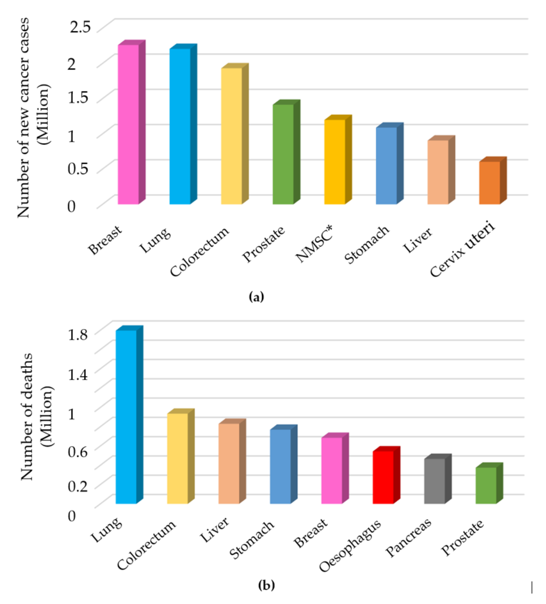
Figure 2.
Changes in 5-year survival rates according to the stage at which lung cancer is detected.
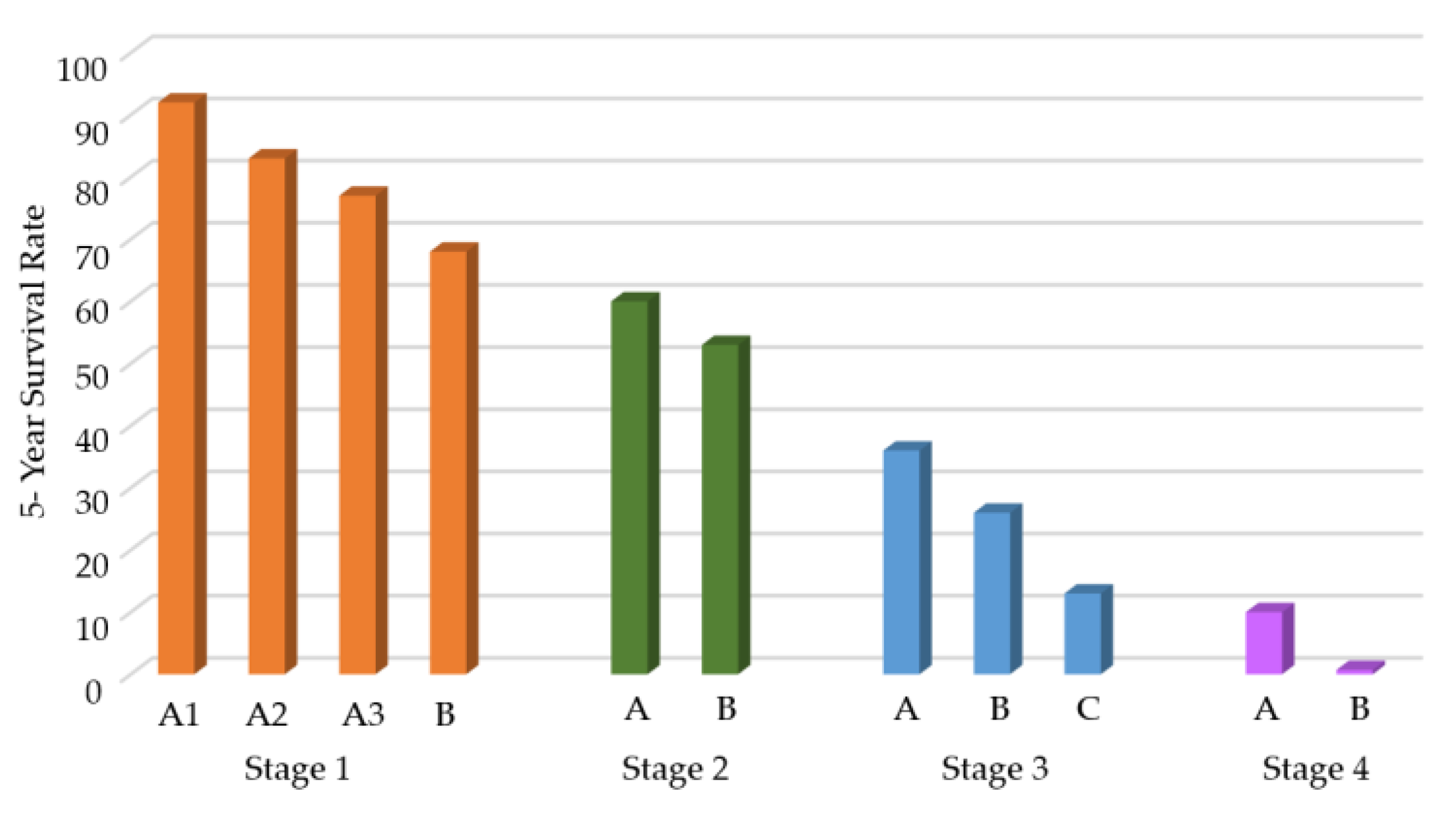
Figure 3.
An illustrative diagram displaying the structure of the mammalian nose in comparison with an e-nose.
Figure 3.
An illustrative diagram displaying the structure of the mammalian nose in comparison with an e-nose.
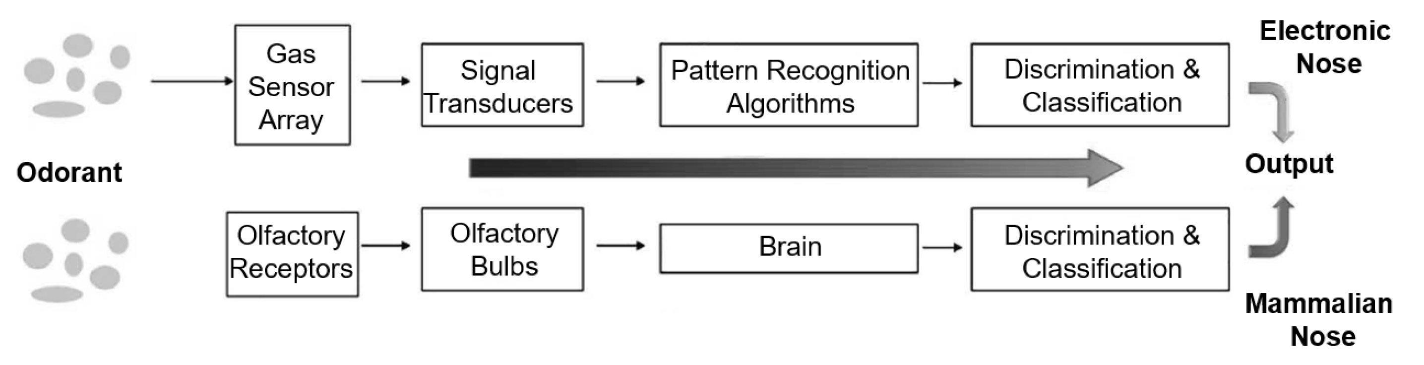
Figure 4.
Schematic representation of the e-nose circuit.
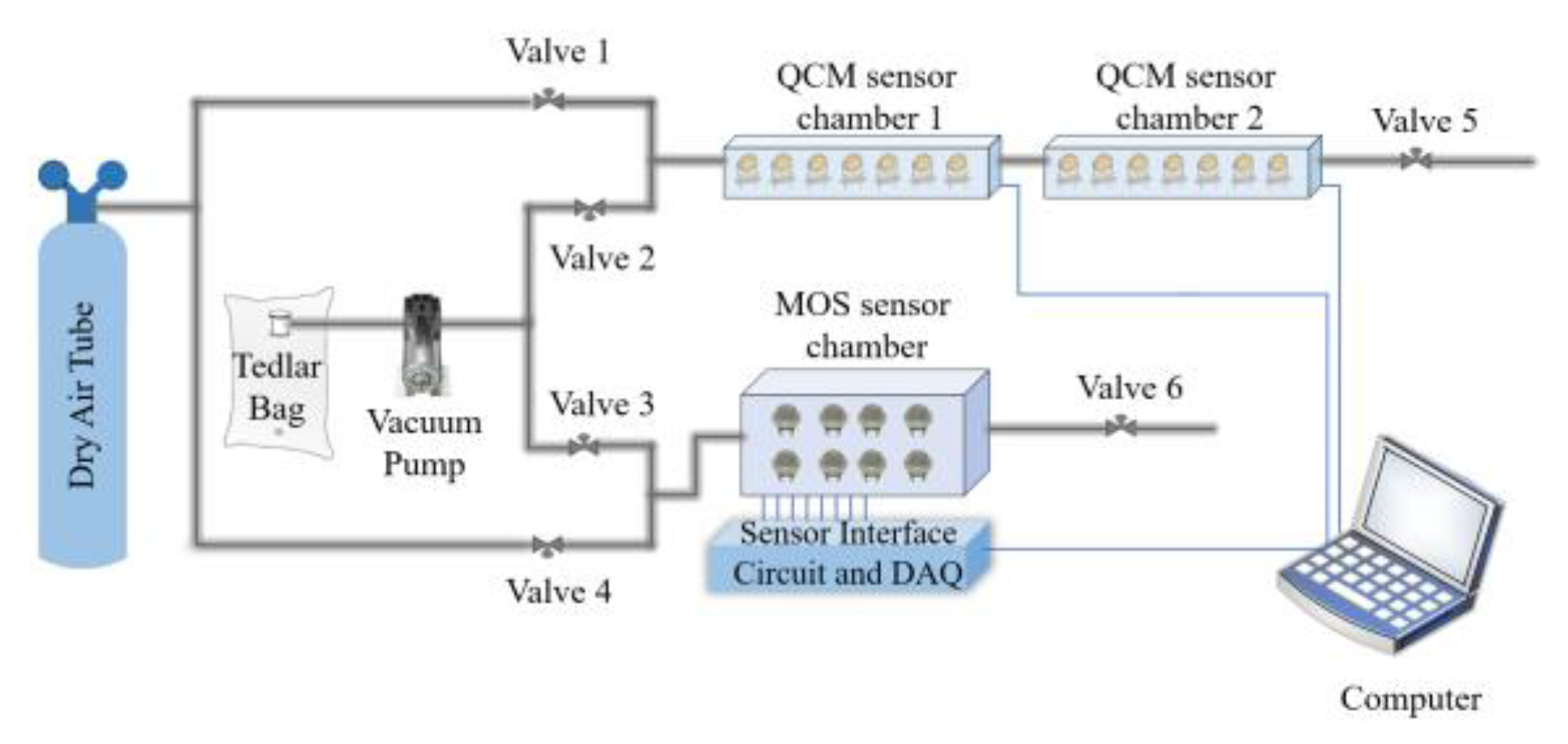
Figure 5.
MOS sensors and their target gases.
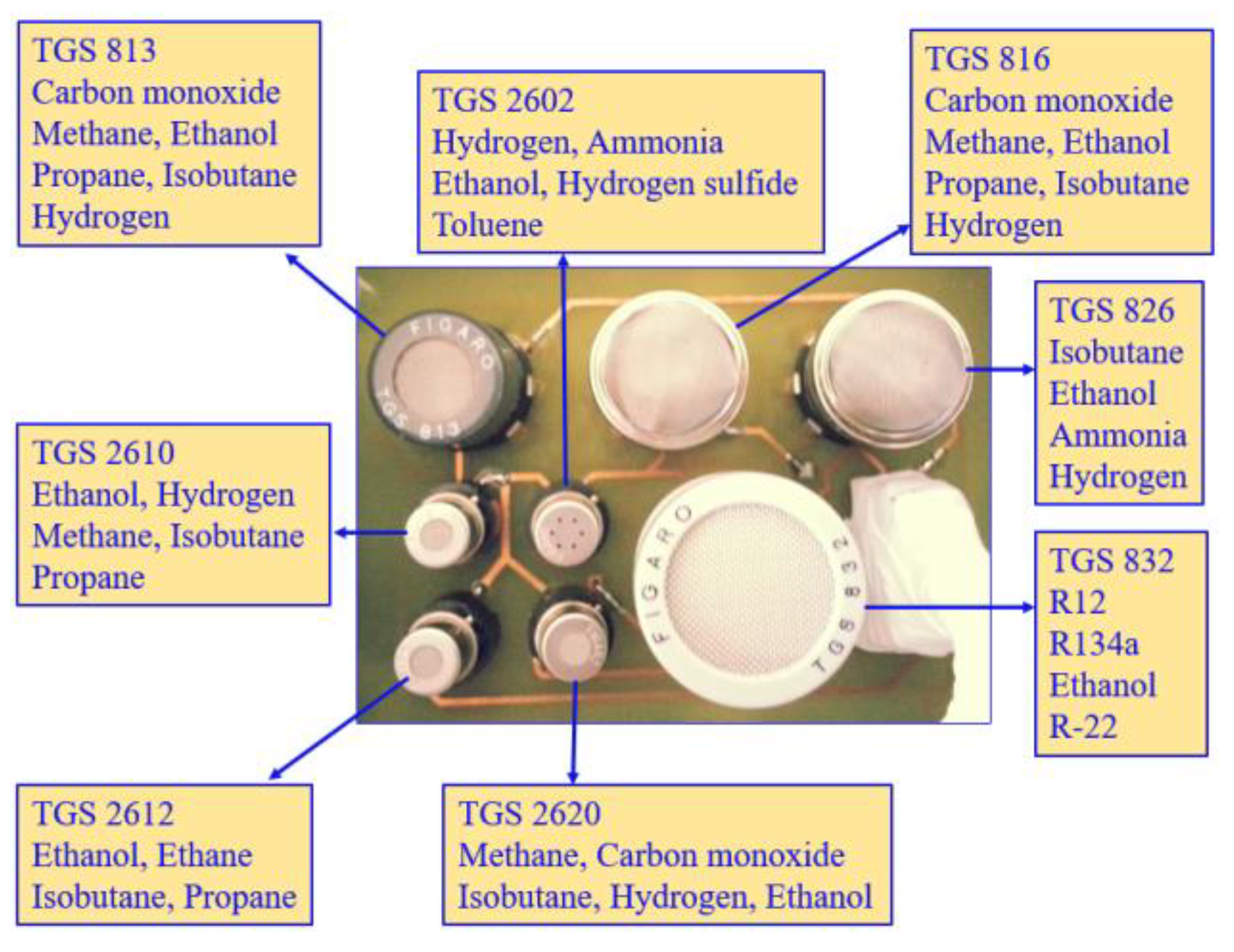
Figure 6.
QCM sensor chamber.
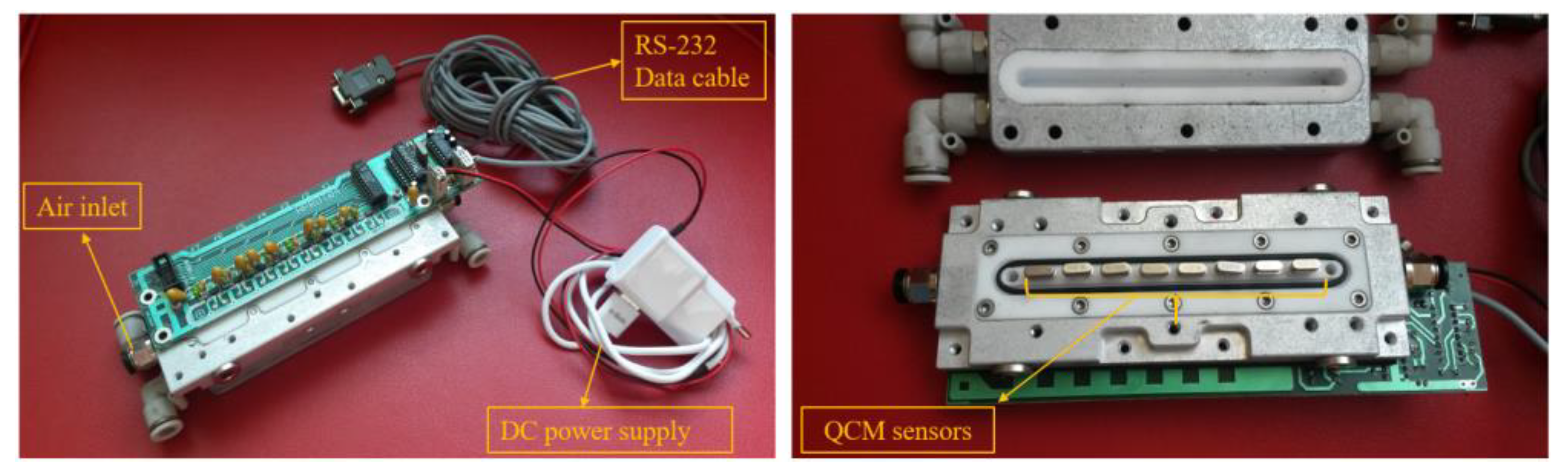
Figure 7.
QCM and MOS sensors utilized in this study.
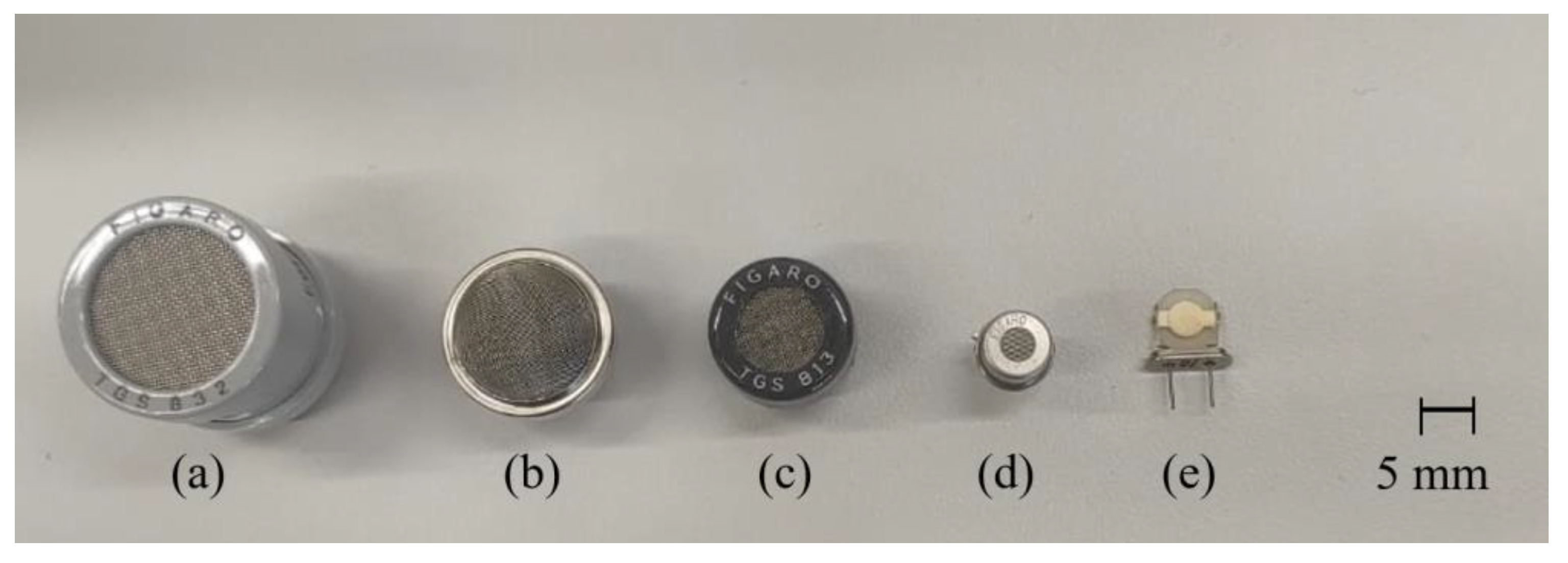
Figure 8.
Developed e-nose circuit.
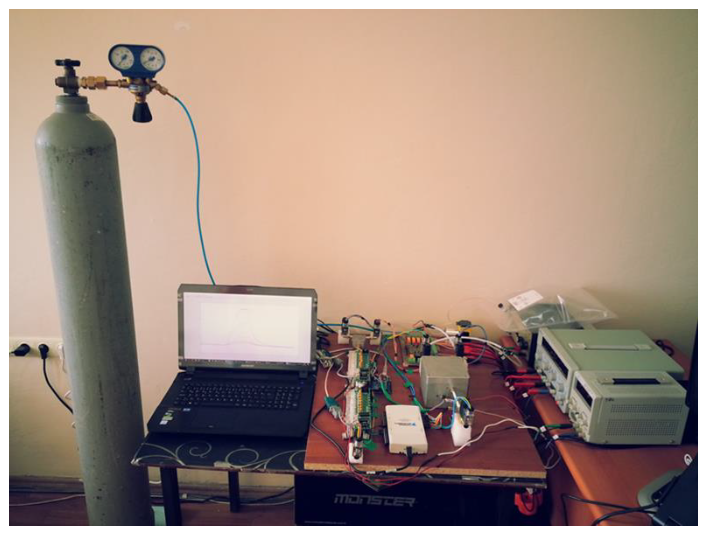
Figure 9.
(a) The signals of the MOS sensor and (b) QCM sensor generated as a result of the experiment.
Figure 9.
(a) The signals of the MOS sensor and (b) QCM sensor generated as a result of the experiment.
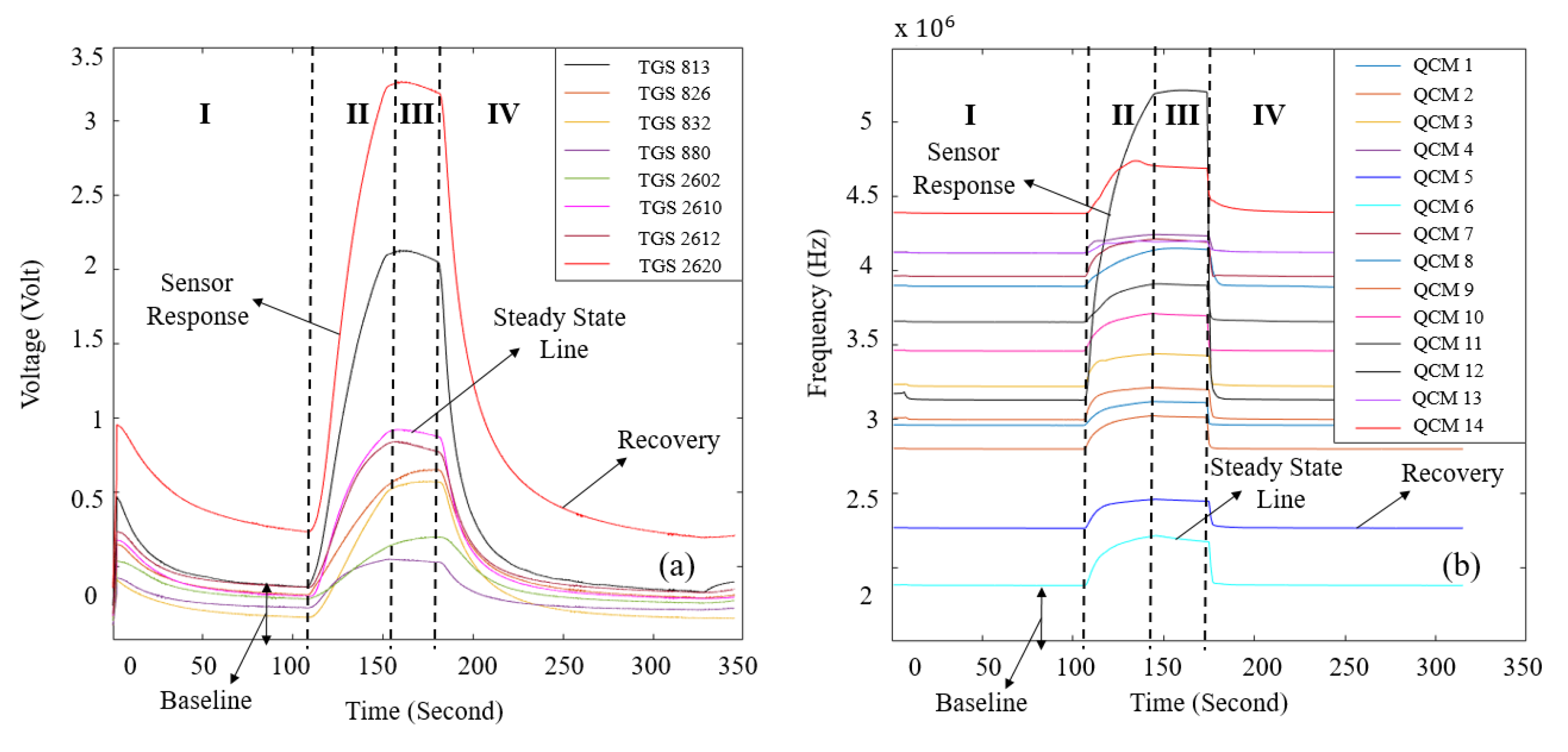
Figure 10.
(a) Distribution of patients based on the histological type of cancer and (b) distribution of patients according to the cancer stage.
Figure 10.
(a) Distribution of patients based on the histological type of cancer and (b) distribution of patients according to the cancer stage.
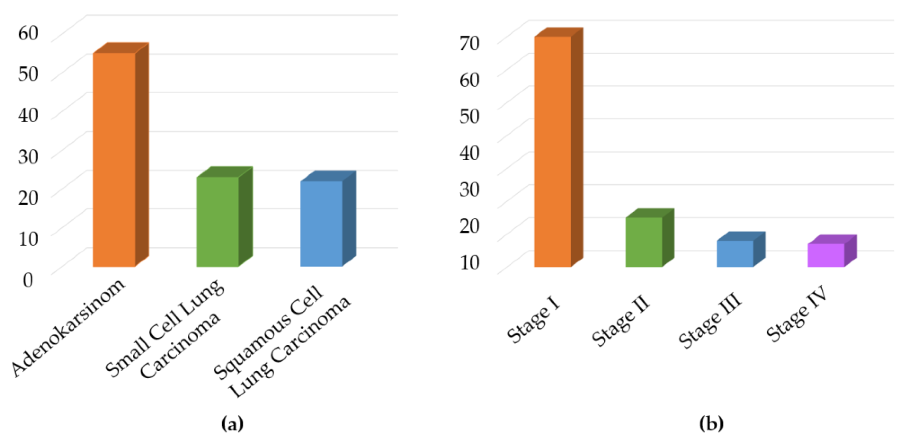
Figure 11.
(a) Raw data; (b) conductivity data of MOS sensors.
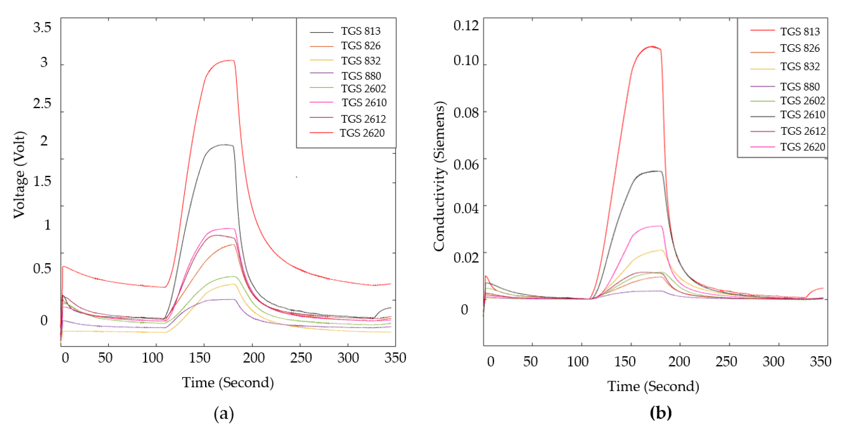
Figure 12.
Scatter plot of the first two features of the dimension-reduced hybrid feature matrix, (a) the dimension of which is reduced by PCA; (b) the dimension of which is reduced by LDA.
Figure 12.
Scatter plot of the first two features of the dimension-reduced hybrid feature matrix, (a) the dimension of which is reduced by PCA; (b) the dimension of which is reduced by LDA.
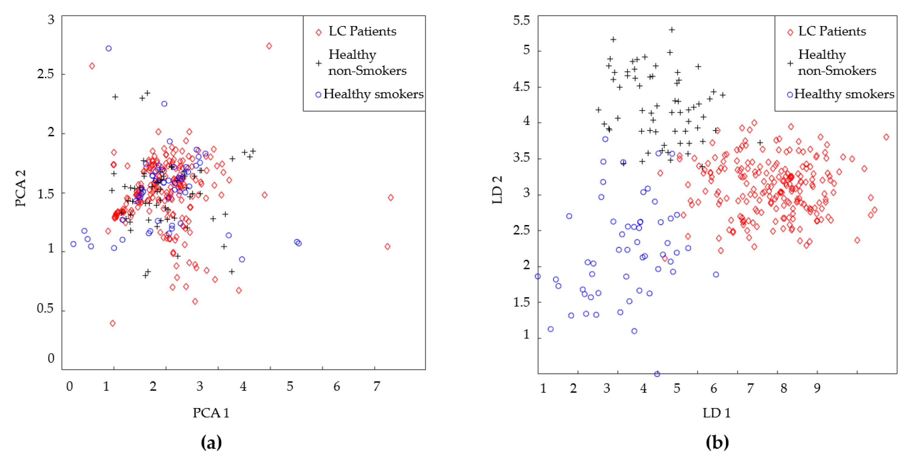
Figure 13.
Confusion matrices obtained as a result of classification of (a) MOS, (b) QCM, (c) MOS+QCM feature matrices.
Figure 13.
Confusion matrices obtained as a result of classification of (a) MOS, (b) QCM, (c) MOS+QCM feature matrices.
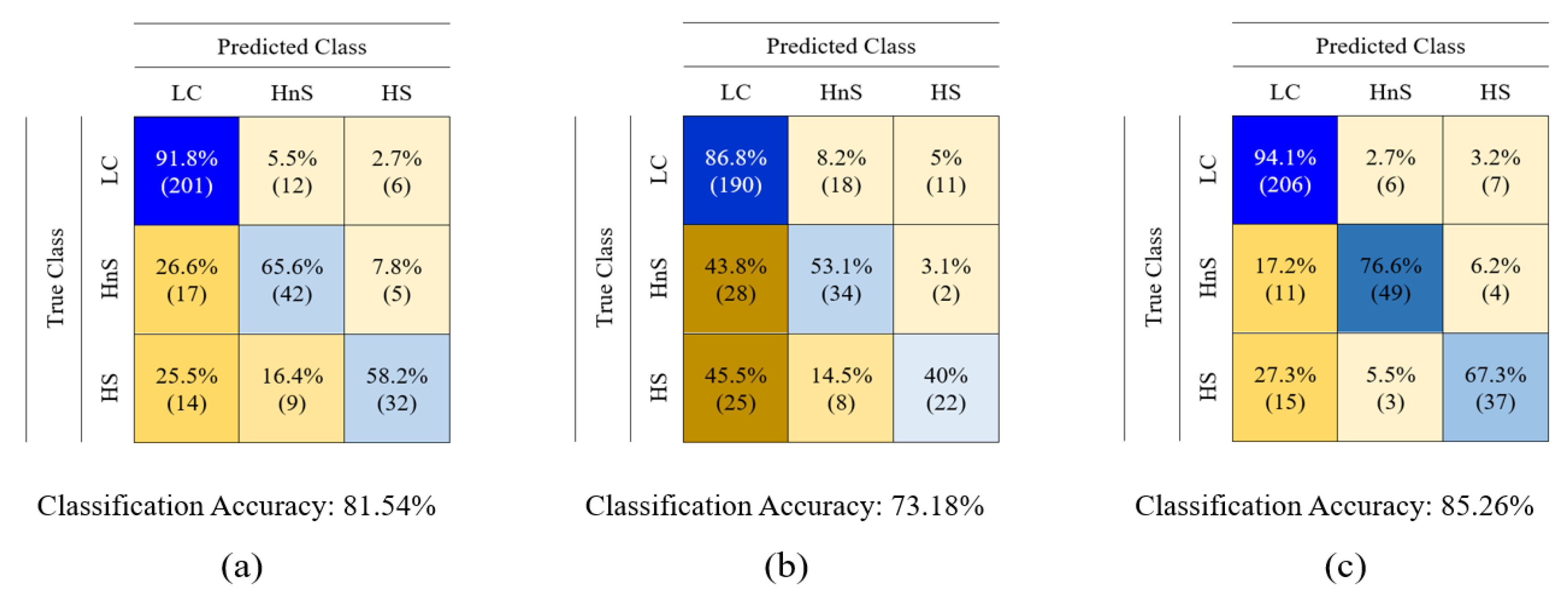
Figure 14.
Confusion matrices obtained as a result of classification of (a) PCA(MOS), (b) PCA(QCM), (c) PCA(MOS+QCM) feature matrices.
Figure 14.
Confusion matrices obtained as a result of classification of (a) PCA(MOS), (b) PCA(QCM), (c) PCA(MOS+QCM) feature matrices.
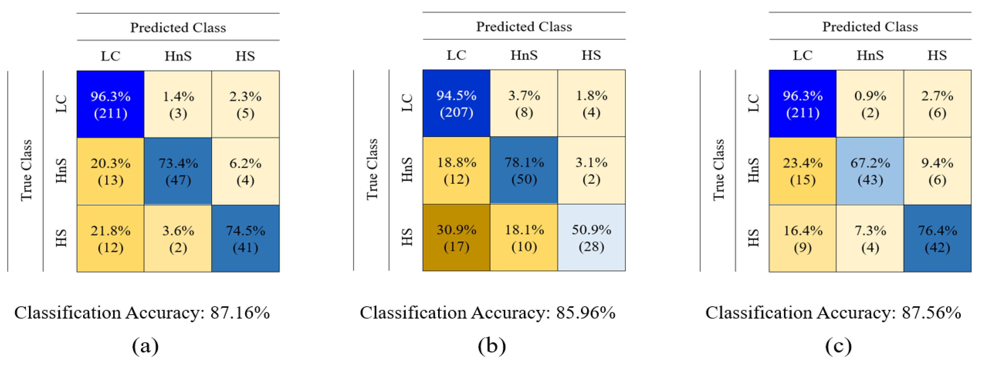
Figure 15.
Confusion matrices obtained as a result of classification of (a) LDA(MOS), (b) LDA(QCM), (c) LDA(MOS+QCM) feature matrices.
Figure 15.
Confusion matrices obtained as a result of classification of (a) LDA(MOS), (b) LDA(QCM), (c) LDA(MOS+QCM) feature matrices.
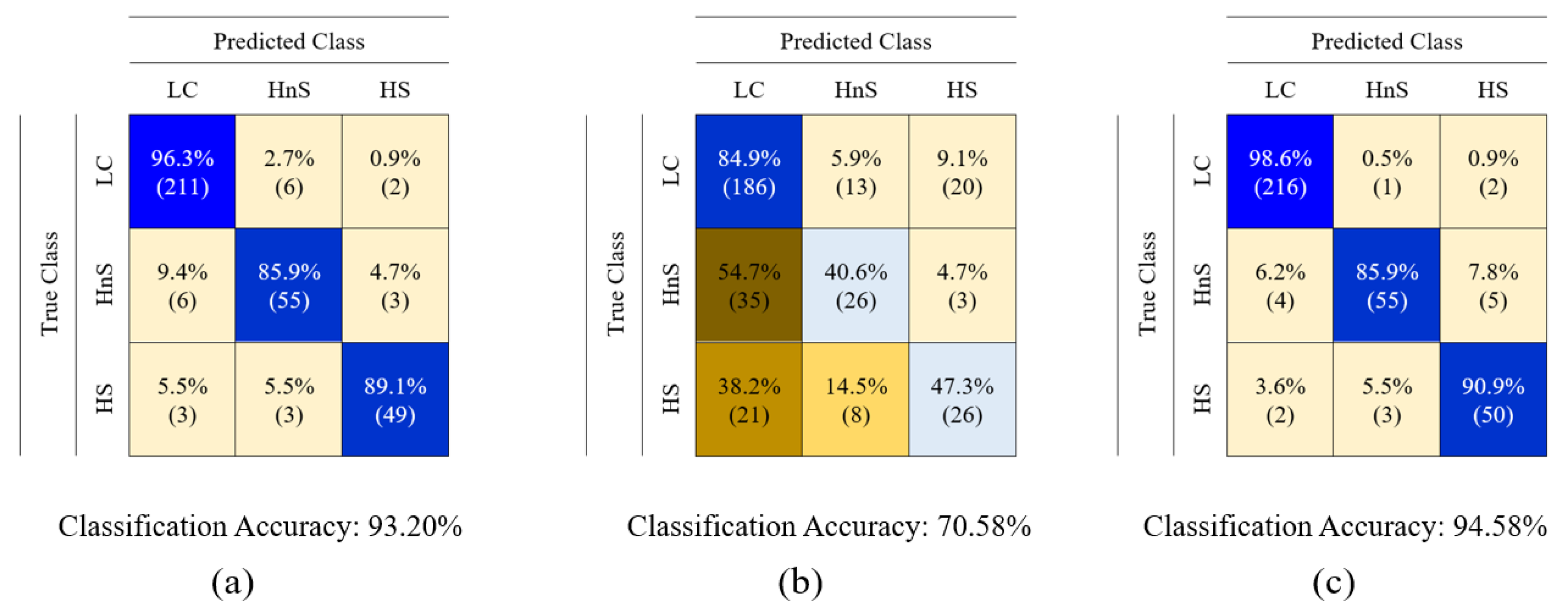
Figure 16.
The initial placement of fuzzy sets on the scatter plot.
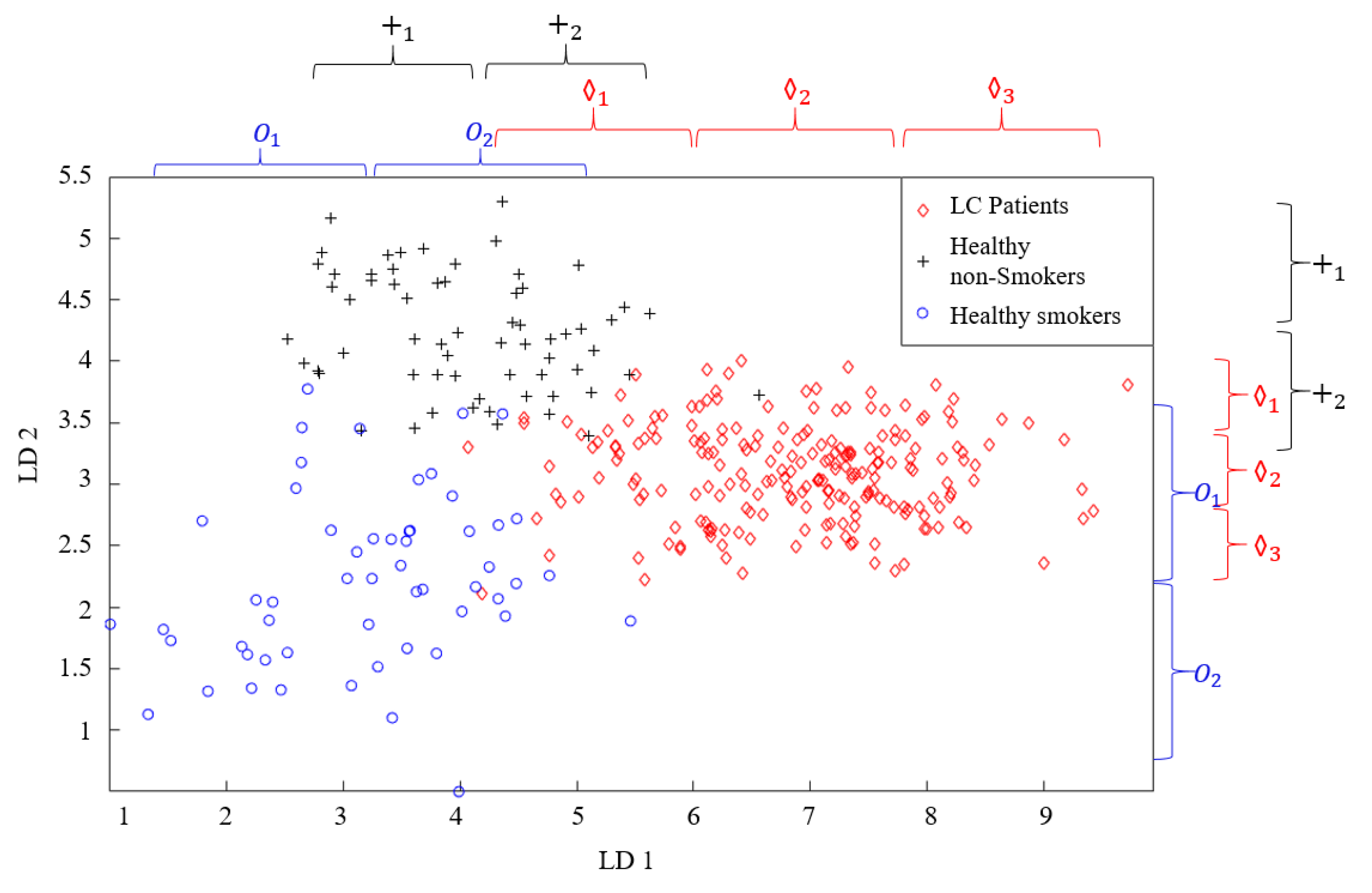
Figure 17.
Optimizing the parameters of fuzzy sets.
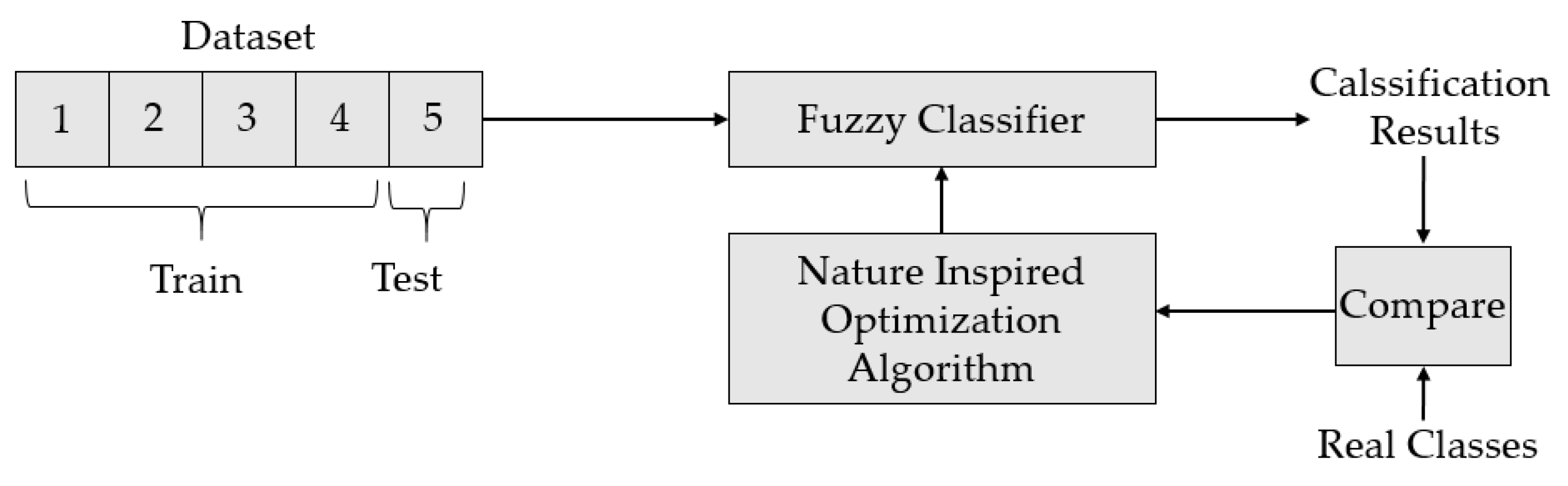
Figure 18.
Placement of optimized generalized bell-shaped membership functions on the scatter plot.
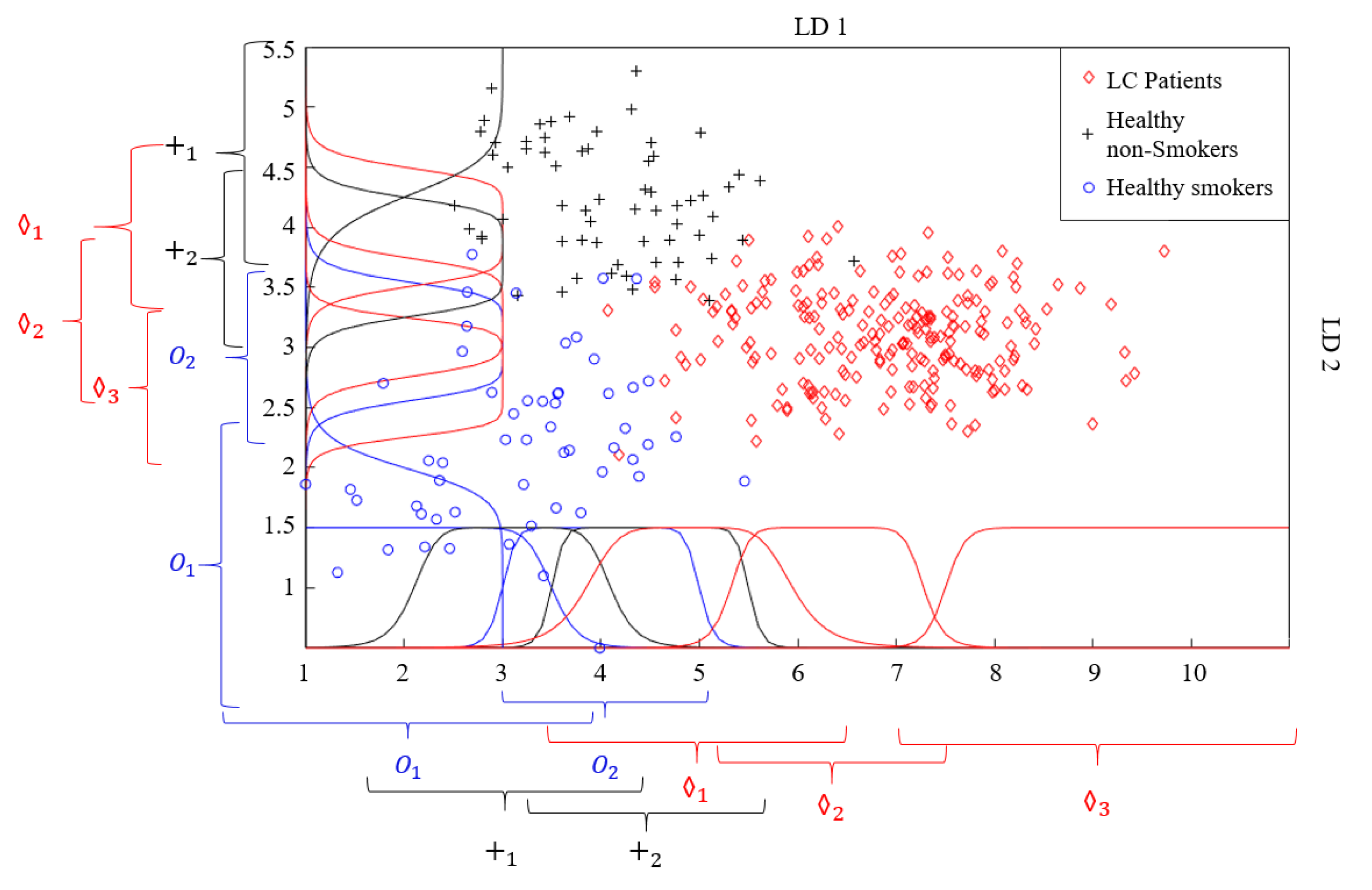
Figure 19.
Performance of gaussian membership function on classification accuracy.
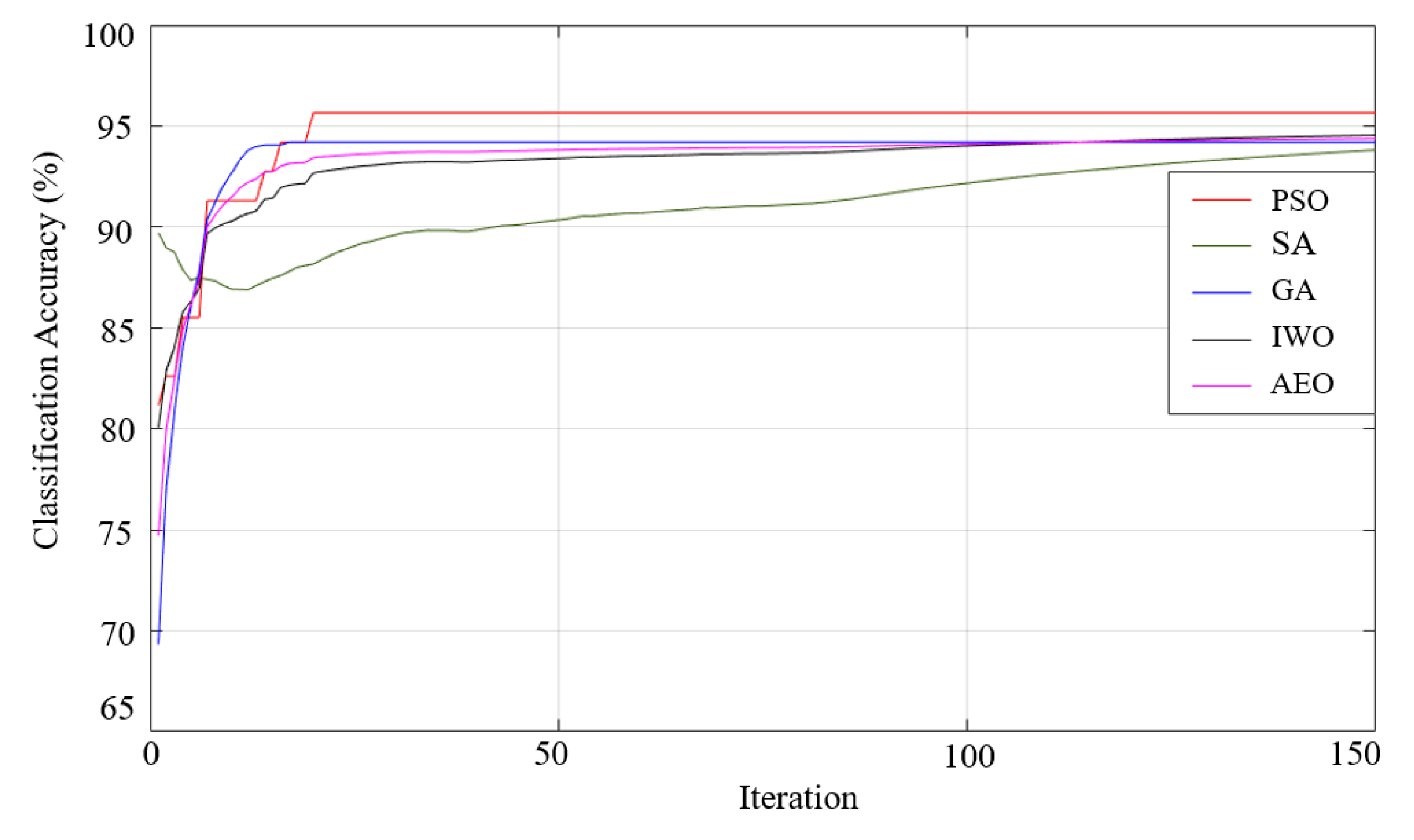
Figure 20.
Performance of generalized bell-shaped membership function on classification accuracy.
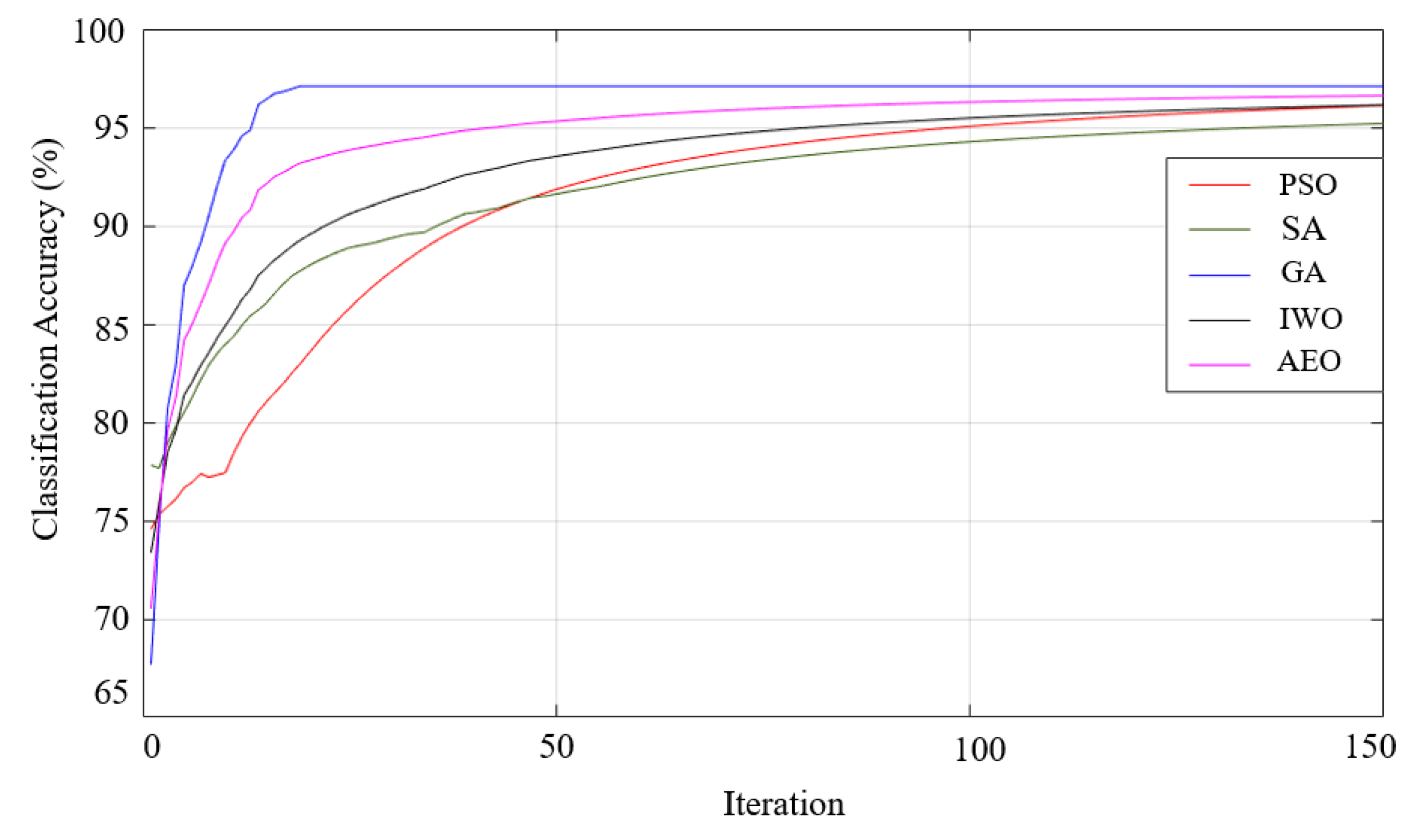
Figure 21.
Performance of pi-shaped membership function on classification accuracy.
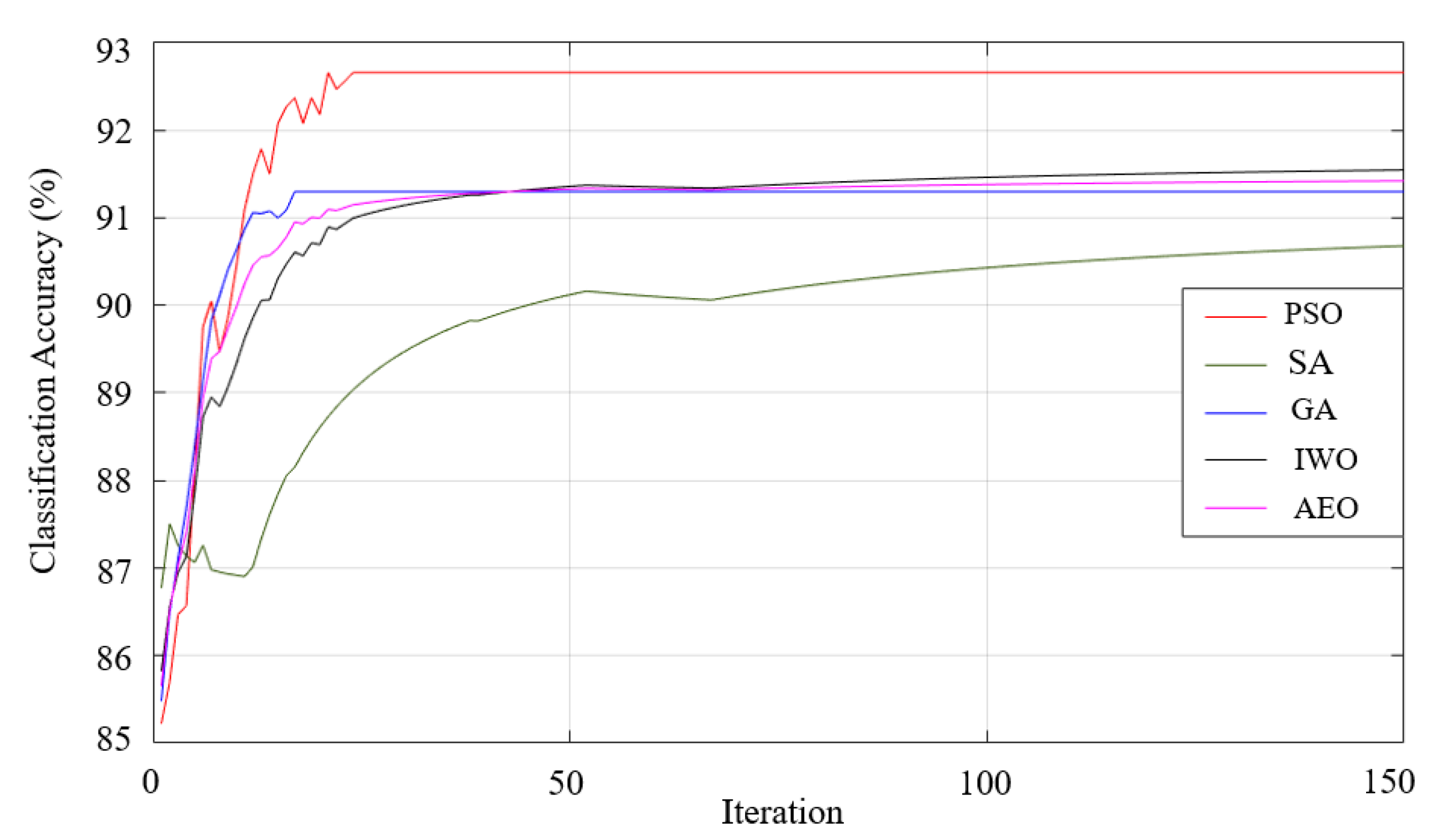
Figure 22.
Performance of trapezoidal membership function on classification accuracy.
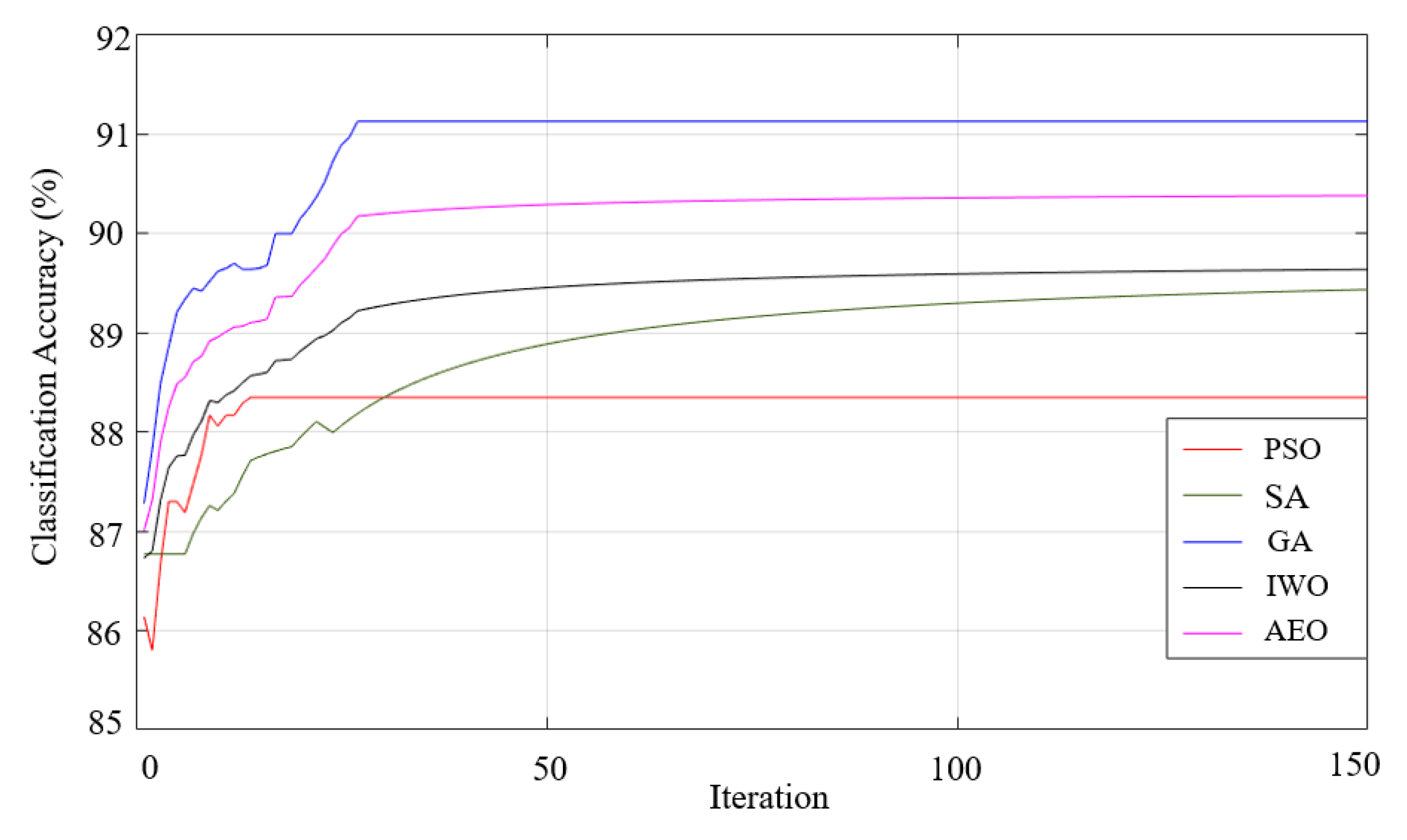
Figure 23.
Performance of triangular membership function on classification accuracy.
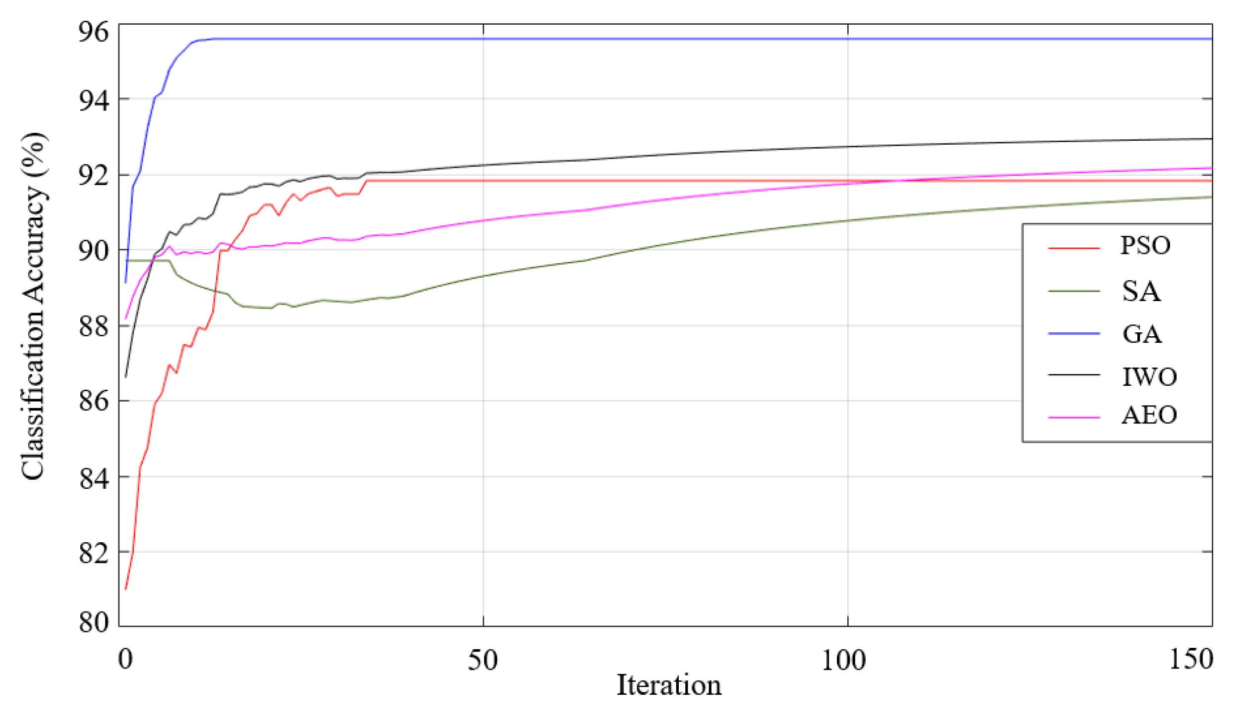
Figure 24.
A graphical comparison of classification accuracies across different methods.
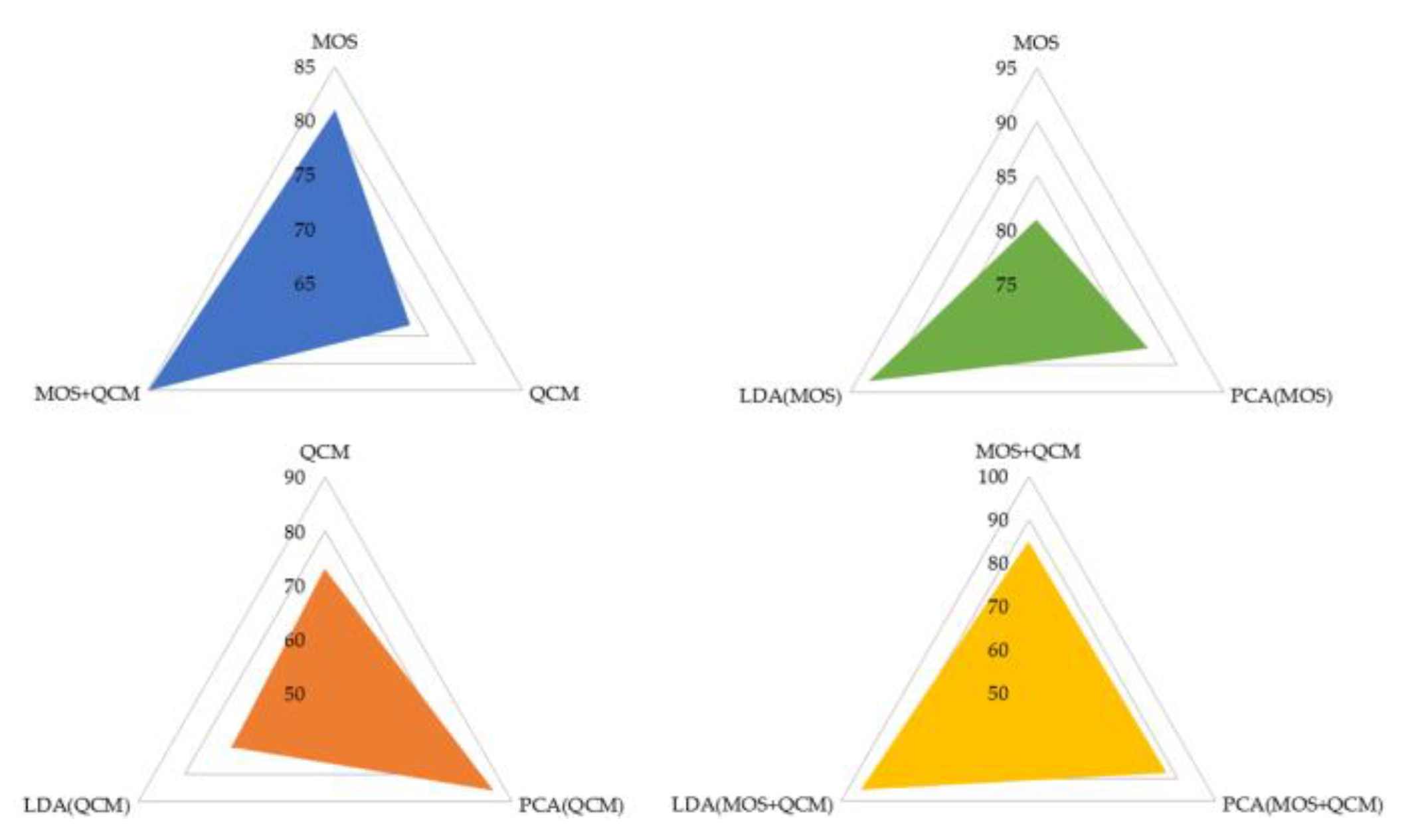
Figure 25.
A comparative visualization of the classification performance across different method (a) Gaussian, (b) Bell-shaped, (c) Pi-shaped, (d) Trapezoidal, (e) Triangular, (f) mixed representation.
Figure 25.
A comparative visualization of the classification performance across different method (a) Gaussian, (b) Bell-shaped, (c) Pi-shaped, (d) Trapezoidal, (e) Triangular, (f) mixed representation.
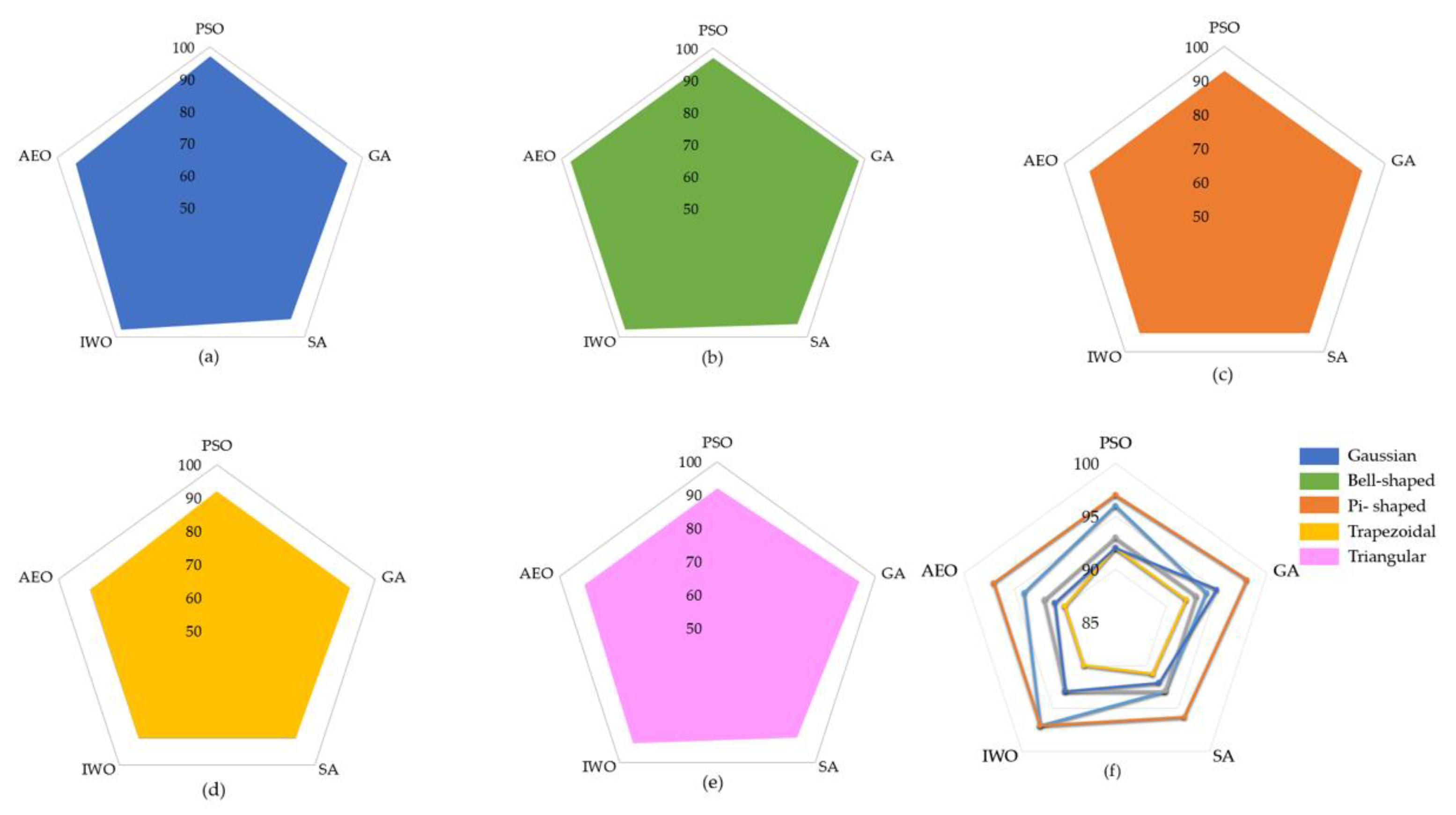

Table 1.
Informative data of the whole volunteers.
| LC patient (60 Person) | Healthy volunteer (40 Person) | |
|---|---|---|
| Age (Mean / St. deviation) | 60.7 / 8 | 48.2 / 9 |
| Gender (Female / Male) | 13/47 | 10/30 |
| Smokers / Non-smokers | 0/60 | 20/20 |
| Ex-smokers | 45/60 | 0/40 |
Table 2.
The classification results.
| Types of features | Classification algorithms | |||||
|---|---|---|---|---|---|---|
| DT | L-SVM | Q-SVM | C-SVM | k-NN | RF | |
| MOS | 75,34 77,8-72,8-1,90 |
75,52 77-74,6-1,08 |
81,12 82,1-79,3-1,17 |
81,28 82-79,3-1,12 |
74,3 79,9-71,3-3,30 |
81,54 82,8-79,9-1,09 |
| PCA(MOS) | 85,20 86,1-84,3-0,67 |
67,86 70,2-64,9-2,17 |
67.66 70,2-64,9-2,11 |
85.76 86,4-84,9-0,62 |
81,06 81,9-79,6-0,90 |
87,16 88,1-86,1-0,88 |
| LDA(MOS) | 88,80 90,1-87,3-1,11 |
93.20 93,1-91,3-0,78 |
92,60 92,9-91,7-0,45 |
91,56 92,8-90,2-1,06 |
90,10 90,8-89,4-0,51 |
90,04 90,8-89,1-0,80 |
| QCM | 66,82 70,7-64,2-2,70 |
64,32 64,8-64-0,43 |
71,96 74,0-70,1-1,46 |
69,66 73,4-66,5-2,51 |
70,50 72,2-68,9-1,33 |
73,18 75,1-70,7-1,77 |
| PCA(QCM) | 74.96 76,9-73,7-1,25 |
67,86 70,2-64,9-2,17 |
67.66 70,2-64,9-2,11 |
82,22 84,3-79,3-1,93 |
85.96 87-84,9-0,89 |
80,20 81,0-79-0,87 |
| LDA(QCM) | 67,30 68,6-65,7-1,30 |
67,86 70,2-64,9-2,17 |
67.66 70,2-64,9-2,11 |
68,92 70,1-68-0,78 |
66,76 70,4-63,3-2,95 |
70,58 71,2-69,9-0,56 |
| MOS+QCM | 76,06 77,8-74-1,43 |
76,84 77,8-75,4-0,96 |
85,26 86,4-83,7-1,05 |
85,18 86,1-84,1-0,79 |
75,38 76-74,9-0,48 |
82,24 82,9-81,4 0,58 |
| PCA (MOS+QCM) |
84,24 84,9-83,4-0,60 |
67,86 70,2-64,9-2,17 |
67,66 70,2-64,9-2,11 |
81,46 82,2-80,8-0,63 |
80,36 85,8-75,4-4,18 |
87,56 88,1-87,2-0,35 |
| LDA (MOS+QCM) |
94,40 94,7-93,8-0,36 |
94,52 94,7-94,4-0,16 |
93,80 94,7-92,9-0,73 |
92.90 94,1-91,6-0,97 |
92,30 93,8-91,4-0,95 |
94,58 95,6-94,1-0,62 |
| PCA(MOS)+ PCA(QCM) |
83,40 85,2-82,0-1,33 |
67,86 70,2-64,9-2,17 |
70,02 70,7-69,2-0,56 |
83,10 83,7-82,2-0,60 |
88,56 88,8-88,2-0,25 |
87,14 88,2-86,10-0,77 |
| LDA(MOS)+ LDA(QCM) |
89,80 90,5-88,9-0,65 |
93,08 93,8-92-0,75 |
92,60 93,8-92-0,73 |
90,74 91,4-89,6-0,80 |
90,60 90,5-89,6-0,35 |
90,92 91,4-90,2-0,54 |
Table 3.
Rule table for classification with FL algorithm.
| LD1 | ||||||||
| LD2 | ||||||||
Table 4.
Membership functions and their details.
| Membership Function | Graph and equation of membership function |
|---|---|
| Gaussian membership function | 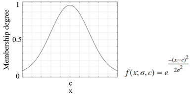 |
| Generalized bell-shaped membership function | 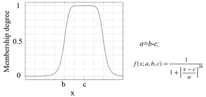 |
| Triangular membership function | 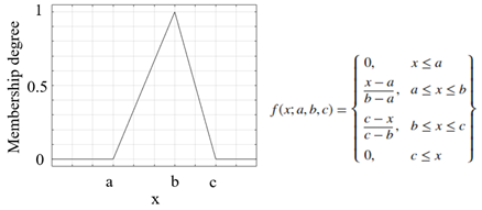 |
| Trapezoidal membership function | 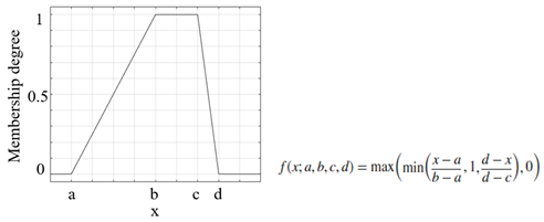 |
| Pi-shaped membership function |  |
Table 5.
Classification of optimization algorithms.
| Algorithm | Tuning parameters | Operators |
|---|---|---|
| GA | Crossover rate | Selection crossover rate, Crossover mutation |
| PSO | Social acceleration coefficient, Inertia weight, cognitive acceleration coefficient | Particle velocity update, Particle position update |
| SA | Temperature | Annealing process |
| AEO | Energy transfer mechanism, | Production,Consumption,Decomposition, Reproduction |
| IWO | Invasive weed spread | Spectral spread, Competitive deprivation |
Table 6.
Parameters and operators of optimization algorithms.
| Algorithm | Source of inspiration | Number of solutions | Nature of algorithm |
|---|---|---|---|
| GA | Biology | Multiple | Stochastic |
| PSO | Biology | Multiple | Stochastic |
| SA | Physics | Single | Stochastic |
| AEO | Biology | Multiple | Stochastic |
| IWO | Biology | Multiple | Stochastic |
Table 7.
Classification results based on the fuzzy logic method.
| Membership Functions |
Optimization Algorithms | ||||
|---|---|---|---|---|---|
| PSO | GA | SA | IWO | AEO | |
| Gaussian | 95.69 98.07-92.80-2.41 |
94.81 97.95-92.07-2.27 |
92.95 97.36-87.22-3.77 |
97.27 98.81-94.71-1.66 |
93.82 97.06-91.18-2.18 |
| Generalized Bell-shaped |
97.27 99.26-95.30-1.72 |
97.93 100-95.89-1.75 |
95.7 99.11-92.62-2.29 |
97.44 98.56-95.59-1.49 |
97.56 98.56-95.59-1.37 |
| Pi | 92.98 97.06-91.18-2.33 |
92.79 97.06-91.18-2.43 |
92.94 97.06-91.18-2.39 |
93.23 97.06-91.18-2.23 |
92.65 97.06-91.05-2.54 |
| Trapezoidal | 91.74 97.06-88.41-3.35 |
92.01 97.06-89.56-3.07 |
90.79 97.06-86.67-3.79 |
89.95 97.06-86.68-4.22 |
90.3 97.06-86.77-3.95 |
| Triangular | 92.3 95.59-89.55-2.22 |
94.81 95.59-92.07-2.27 |
91.62 95.59-89.71-2.51 |
92.7 97.06-9.71-2.77 |
91.47 95.59-89.56-2.63 |
Disclaimer/Publisher’s Note: The statements, opinions and data contained in all publications are solely those of the individual author(s) and contributor(s) and not of MDPI and/or the editor(s). MDPI and/or the editor(s) disclaim responsibility for any injury to people or property resulting from any ideas, methods, instructions or products referred to in the content. |
© 2025 by the authors. Licensee MDPI, Basel, Switzerland. This article is an open access article distributed under the terms and conditions of the Creative Commons Attribution (CC BY) license (http://creativecommons.org/licenses/by/4.0/).
Copyright: This open access article is published under a Creative Commons CC BY 4.0 license, which permit the free download, distribution, and reuse, provided that the author and preprint are cited in any reuse.


