Submitted:
21 July 2025
Posted:
22 July 2025
You are already at the latest version
Abstract
Poor air quality can harm human health and the environment. Air quality data is needed to understand and reduce exposure to air pollution. Air sensor data can sup-plement national air monitoring network data to better understand localized air qual-ity and trends. However, these sensors can have limitations, biases, and inaccuracies that must first be controlled to generate data of adequate quality. Analyzing sensor data requires not only a background knowledge of air quality but also often requires extensive data analysis skills which may require new skills or time that burdens many air agencies (e.g., small states, local). To address these issues, an R-Shiny application has been developed to assist air quality professionals in 1) understanding air sensor data quality through comparison with nearby ambient air reference monitors, 2) ap-plying basic quality assurance (QA) and quality control (QC), and 3) understanding local air quality conditions. This tool provides agencies with the ability to more quickly analyze and utilize air sensor data for a variety of purposes while increasing the re-producibility of analyses. This paper highlights a case study using the tool to explore sensor performance during Canadian wildfire smoke impacts in the midwestern United States during June of 2023.
Keywords:
air sensor
; data analysis
; open source
; air quality
1. Introduction
Poor air quality is associated with a variety of negative health effects [1]. Air quality data are needed to understand local conditions and reduce exposure to air pollution [2]. In the U.S., air quality is measured by ambient air monitors operated by state, local, and Tribal air agencies [3]. Recent efforts supplement the national monitoring network with localized air sensor data to investigate variations in air quality at neighborhood scales. Air sensors typically cost one or two orders of magnitude less than conventional air monitors (e.g., $10-$10k) and are designed to be compact enabling additional measurements at more locations. However, air sensor data may be noisy [4,5], biased, or inaccurate [6]. Furthermore, sensor performance may vary over time [7], concentration range (e.g., nonlinear response), or the environment in which they operate (e.g., high relative humidity, RH) [8,9]. Limitations may be pollutant, sensor technology (e.g., optical, electrochemical, metal oxide), or manufacturer specific and quality assurance (QA) and quality control (QC) steps must be tailored for the specific sensor needs [10]. Sensors often must be compared with nearby measurements and corrected to improve the data quality [11,12,13,14]. The air sensor data analysis required to account for these limitations is challenging for users without extensive coding experience and for agencies faced with increased data volumes and community questions and with steady or decreasing staff time.
Many existing air data analysis software tools are costly; require coding experience to be run in an open-source environment [15,16,17]; are specific to one manufacturer’s sensor [16,18]; or are designed to focus on single collocation sites [19]. An analysis tool is needed to more easily aggregate data from multiple air quality data sources, perform standard QC, identify nearby sensors spatially for comparison, and create comprehensive visualizations. Generating air quality analysis in this form will further the capabilities of air sensors and potentially aid in protecting public health and the environment.
2. Materials and Methods
The Air Sensor Network Analysis Tool (ASNAT) is an R-Shiny [20,21] application that integrates data from multiple air quality networks (e.g., national monitoring network, sensor networks, meteorological stations) to provide a broader representation of local air quality. The tool was developed mostly in R with some code in C++ to enhance performance speed. It was designed to support air quality professionals with a base knowledge of air quality analysis to develop sensor data corrections, apply data flagging, understand the performance of new air sensor networks, and improve sensor data quality so that the comparability between networks is improved and users can better understand local air quality - including during extreme events like wildfires, dust storms, and fireworks.
Users can select data from EPA’s Remote Sensing Information Gateway (RSIG) (under “Load Web” in Figure 1) which allows users to efficiently call data based on a geographic bounding box. Users can retrieve AirNow, EPA’s Air Quality System (AQS), Meteorological Aerodrome Report (METAR), and public crowdsourced PurpleAir data [22] (https://www.epa.gov/hesc/web-access-rsig-data, last accessed 2/28/25) ). Data from AirNow and AQS available in ASNAT include fine particulate matter (PM2.5), particulate matter 10 µm or less in diameter (PM10), RH, temperature, pressure, ozone (O3), nitrogen dioxide (NO2), carbon monoxide (CO), and sulfur dioxide (SO2). While the AQS and AirNow datasets are similar, the AQS dataset has gone through further QA and QC and typically it will not be available for a few months after it has been collected. In some cases, more data may be included in the AirNow dataset as not all monitors also report to AQS. Depending on the application, AirNow or AQS data may be more appropriate, and users can easily run analysis with one and then the other. The PurpleAir dataset includes the corrected PurpleAir PM2.5 data (PurpleAir.pm25_corrected) that is corrected in a similar way as PurpleAir data on the EPA and US Forest Service AirNow Fire and Smoke Map (fire.airnow.gov, accessed: 1/28/25) including completeness criteria (70% for daily or hourly averages), exclusion when A and B channel measurements disagree, and application of the US-wide correction that accounts for nonlinearity at high smoke concentrations [23]. Users must supply a valid PurpleAir API read key (available directly from PurpleAir) to access this data. Users can also load data from standard format text files, which can be generated using the Air Sensor Data Unifier tool (https://www.epa.gov/air-sensor-toolbox/air-sensor-data-tools, last accessed 2/28/25), or from offline PurpleAir files. Data can be loaded at hourly or 24-hour averages and NowCast averaging can also be applied to visualizations and statistics (https://usepa.servicenowservices.com/airnow/en/how-is-the-nowcast-algorithm-used-to-report-current-air-quality?id=kb_article&sys_id=798ba26c1b1a5ed079ab0f67624bcb6d, last accessed 20 June, 2025).
Throughout this paper we will use a 2-week case study to demonstrate the features and functionality of this tool. During June 2023, the midwestern U.S. was impacted by smoke from Canadian wildfires [24]. During uncommon events like these, state and local agencies may be interested in better understanding how sensors perform and whether any improved QA QC is needed to provide accurate data to the public. Further, the synthesis of air quality data from multiple observational networks supports current and future agency response (e.g., publicizing current air quality conditions and suggested response, documenting evidence of exceptional events).
3. Results
ASNAT provides a variety of ways for users to view and explore local air quality. Once users select and load data, monitoring sites appear on the map at the top of the map tab (Figure 1). Each data type is assigned a symbol, and users select a colormaps that is then described in the legend. Users can choose how to view the data (hourly averages, nowcast averages, daily averages, mean value over all time steps) and use the timestep slider below the map to animate the information, if applicable (Figure 1).
Currently ASNAT has six tabs that provide different ways to interact with the data. These include the map, flagging, tables, plots, corrections, and network summary tabs. After selecting data, users can decide to either move to the flagging tab or to the plots tab. In many cases the user may need to generate the tables and plots before deciding what kind of flagging and removal of problematic data is needed.
If the user has selected only an X variable, the tables tab summarizes the data by site ID including the count (i.e., number of hours or number of days available), percent of missing data, mean, minimum, 25th percentile, median, 75th percentile, and maximum. If the users have selected X and Y variables within a certain distance it provides the same summary table for each X and Y variables. In addition, it provides a table of the neighboring points at each time stamp, the coefficient of determination (R2) and distances between each set of points, and the number of points in each air quality index (AQI) category and the normalized mean bias error (NMBE), root mean squared error (RMSE), and normalized root mean squared error (NRMSE) in each AQI category. If the user generates these tables and then uses the save data button, these summary tables will be saved along with the raw data.
The plots and network summary tabs include additional visualizations to understand network performance and local air quality. Figure 2 presents a summary of air quality variation from the network summary tab. During our two-week case study, AQS monitors (red color) report slightly higher concentrations than the PurpleAir sensors (blue color) and show somewhat different time of day patterns. Because some differences were found, users can go on to compare nearby sensor and monitor pairs, instead of all sensors and monitors within the area, to understand whether this is due to sensor bias or because the sensors and monitors are exposed to different pollutant concentrations.
The plots tab allows users to compare two datasets by finding nearest neighbors within a user specified distance. Typically, this involves comparing a sensor dataset with more uncertainty and unknown performance to nearby reference monitor data (e.g., AirNow, AQS) to better understand sensor performance and develop corrections. ASNAT describes the sensor-monitor relationship through a series of performance metric calculated as outlined in EPA’s performance targets [25,26,27,28] (Figure 3, Figure 4).
In this case study example, sensor-monitor pairs within 250 meters were selected. Most sensor-monitor pairs are strongly correlated, meeting EPA’s performance target for coefficient of determination (R2) with only a few pairs falling below the 0.7 target. All sensor-monitor pairs meet the targets for slope (1 ± 0.35), intercept (5 ≤ b ≤ 5 mg/m3), and root mean squared error (RMSE ≤ 7 mg/m3). Some sensors have normalized root mean squared error outside of the target (>30%) however, EPA’s performance targets only require meeting either the RMSE or the NRMSE target.
Using the corrections tab, sensor corrections can also be developed to adjust for bias between the sensor and the monitor (or whatever two comparison variables the user selects). Sometimes, a simple linear correction allows two datasets to become more comparable. However, much past work with air sensors has shown that RH or temperature can influence sensor measurements and that many gas sensors may have cross sensitivities to other gases [9] so a third variable may be needed to account for some of these influences or interferences. In ASNAT, currently available corrections include single variable, multivariable additive, or multivariable interactive in either linear, quadradic, or cubic forms.
Figure 4a shows a sensor with a weak correlation (R2 = 0.57 < 0.7). There are a variety of reasons why this sensor may have weaker performance than the typical sensor during this period (Figure 3). For instance, this sensor may be located closer to a source leading to the higher PurpleAir concentrations reported when the nearby reference monitor (AQS) measurements are low, the user may have improperly reported the latitude and longitude of the sensor meaning the sensor may be more than 250 m from the AQS monitor, differences in federal equivalent method (FEM) may lead to differing performance, this sensor may have hardware or software differences leading to different performance, or there may be other issues. Figure 4b shows a different sensor has strong agreement and low normalized mean bias error (NMBE) when compared to the nearby reference monitor. Depending on the project objectives, this performance may be adequate. If higher accuracy is needed, the individual sensor correction generated (y = -1.4597 + 1.1643x) could be applied.
Performance of the sensor can also be explored by considering how frequently the sensors and monitors report the same AQI category (Figure 5) also using the plots tab. This example shows strong agreement with hourly averages agreeing at least 76% of the time across categories. NowCast and 24-hour averages are more frequently used for AQI display but it is typically more challenging for sensors and monitors to agree at shorter averaging intervals (e.g., hourly).
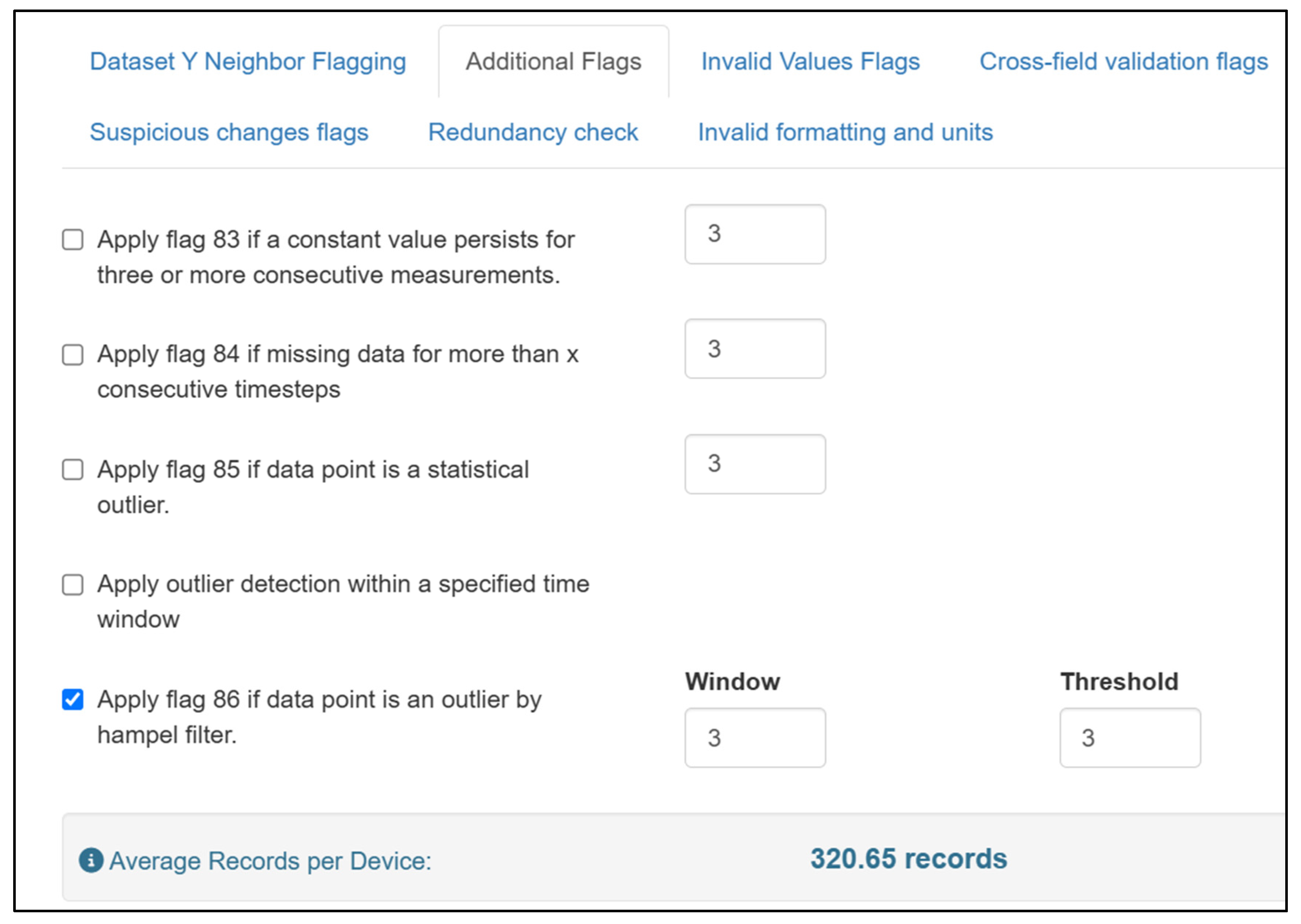
The flagging tab provides a variety of options to flag and/or remove anomalous data based on several categories such as: exceedance of a threshold, agreement with a nearest neighbor, repeated values, outlier detections (using several methods), a user specified period (e.g., a day with a known sensor issue), and more (Figure 6). More than one flag can be applied. Performance plots on the plots tab (i.e., overall scatterplot, AQI agreement plot, boxplots of performance targets) are shown with all data and only the unflagged data and flagged points are indicated in lighter shades on the timeseries. When data is downloaded the flags will be removed. In this case study example, there are no clear outliers to remove.
4. Discussion
The Air Sensor Network Analysis Tool (ASNAT) is an R-Shiny [20,21] application designed to ease the burden of combining, comparing, and summarizing discrete air monitoring networks operating in the same time and place making it easier for air monitoring agencies to understand local air quality. Limitations of this tool include data size limits and the need for users to have some background air quality knowledge to appropriately use and interpret the available tools. Functionality is limited to the most requested analyses. Dataset size limits are dependent on local computing resources. Users may need to limit longer time analysis to smaller spatial ranges and/or longer averaging intervals. Some background air quality knowledge is needed to successfully use this tool and make informed decisions based on ASNAT outputs. For example, nearest neighbor radius will depend on pollutant chemistry, local sources, and geography. Local knowledge may be required to determine if outliers are due to sensor malfunctions or real short-term pollutant events. In addition, more complicated corrections (e.g., machine learning, additional variables) are sometimes required for adequate sensor performance but these more complicated corrections are not currently possible in ASNAT. These more complex corrections can increase the risk of over fitting (i.e., generating a correction model that will not perform adequately outside of the calibration period) [29,30], are not easy to interpret [29], and require longer calibration periods [31]. For these reasons we have not included more complicated corrections currently to hopefully prevent users from generating unhelpful corrections. There will always be additional analysis, quality assurance, or plots that could be helpful to understand local air quality issues, however, this tool gives users without data analysis expertise and those who do a quick way to perform some helpful analysis.
This project is ongoing, and we hope to add additional features and improvements based on the feedback from the initial users. In addition, since the code is open-source and publicly available, we hope that users will take it and modify it as needed for their own uses adding additional functionality and customized displays. So far more than two hundred air quality professionals have been trained to use this tool including staff from state, local, and tribal agencies, EPA, other federal agencies, academia, consulting companies, and other organizations. The high engagement in tool training and office hours highlight the strong need for this type of tool.
This tool contributes to increasing the utility of air sensor data. For example, state agency staff plan to use the tool to help support a community monitoring project using PurpleAir sensors and to perform regression analysis on multiple PurpleAir sensors collocated with an air monitor. Also, they plan to use the tool to use this tool to understand how custom-built sensors compare to nearby PurpleAir sensors. Local agency staff plan to use the tool to understand how local sources (e.g., incinerators) impact air quality at schools. By reducing the time it takes to complete analysis, resources are saved that can be put into furthering these projects or other agency priorities. In addition, this data can be used to take informed actions to better protect public health. This may include providing more accurate data to the public or better understanding local sources.
Author Contributions
Conceptualization, K.K.B.; software, T.P., J.Y., G. P., Y.X., C.S., R.B., and H.N.Q.T.; validation, K.K.B., T.P., J.Y., G.P., Y.X., S.K., C.S., R.B., and H.N.Q.T.; data curation, T.P., A.L.C., and K.K.B.; writing—original draft preparation, K.K.B.; writing—review and editing, T.P., J.Y., G.P., Y.X., S.K., C.S., R.B., H.N.Q.T, S.A., and A.L.C.; visualization, T.P., J.Y., and R.B.; supervision, S.A.; project administration, K.K.B., Y.X., S.A., S.K., and A.L.C.; funding acquisition, K.K.B., S.K., and A.L.C.. All authors have read and agreed to the published version of the manuscript.
Funding
This work was supported by EPA internal funding (Air Climate and Energy National Research Program, Regional-ORD Applied Research Program, and Environmental Modeling and Visualization Laboratory).
Institutional Review Board Statement
Not applicable
Informed Consent Statement
Not applicable
Data Availability Statement
Code is available on github https://github.com/USEPA/Air-Sensor-Network-Analysis-Tool-Public- and operating system specific zip files are available at the following links windows https://ofmpub.epa.gov/rsig/rsigserver?asnat/download/Windows/ASNAT.zip, Mac https://ofmpub.epa.gov/rsig/rsigserver?asnat/download/Darwin.arm64/ASNAT.zip, Mac https://ofmpub.epa.gov/rsig/rsigserver?asnat/download/Darwin.x86_64/ASNAT.zip, and Linux https://ofmpub.epa.gov/rsig/rsigserver?asnat/download/Linux.x86_64/ASNAT.zip.
Acknowledgments
Thank you to PurpleAir for providing data (MTA #1261-19) and to Adrian Dybwad and Amanda Hawkins. Thank you to Heidi Paulsen (EPA), Sedona Ryan (UNC), Stephen Beaulieu (Applied Research Associates), and Eliodora Chamberlain (EPA Region 7) for their project management and other support. Thank you to those who provided input, example datasets, and testing including: U.S. EPA Amara Holder (ORD), Megan MacDonald (ORD), Ryan Brown (Region 4), Daniel Garver (Region 4), Chelsey Laurencin (Region 4), Rachel Kirpes (Region 5), Dena Vallano (Region 9), Laura Barry (Region 9), Nicole Briggs (Region 10), Elizabeth Good (Office of Air Quality Planning and Standards), and Arjun Thapa (ORD former); South Coast Air Quality Management District Wilton Mui, Vasileios Papapostolou, Randy Lam, Namrata Shanmukh Panji, Ashley Collier-Oxandale (former); Washington Department of Ecology Nate May; Puget Sound Clean Air Agency Graeme Carvlin; New Jersey Department of Environmental Protection: Luis Lim; Desert Research Institute: Jonathan Callahan; Asheville-Buncombe Air Quality Agency Steve Ensley; and Oregon Department of Environmental Quality Ryan Porter.
Conflicts of Interest
The authors declare no conflicts of interest.
EPA Disclaimer: The mention of trade names, products, or services does not imply an endorsement by the U.S. Government or the U.S. Environmental Protection Agency. The views expressed in this paper are those of the author(s) and do not necessarily represent the views or policies of the U.S. Environmental Protection Agency.
Abbreviations
The following abbreviations are used in this manuscript:
| AQI | Air Quality Index |
| AQS | Air Quality System |
| ASNAT | Air Sensor Network Analysis Tool |
| CO | Carbon Monoxide |
| EPA | Environmental Protection Agency |
| FEM | Federal Equivalent Method |
| MDPI | Multidisciplinary Digital Publishing Institute |
| METAR | Meteorological Aerodrome Report |
| MTA | Material Transfer Agreement |
| NO2 | Nitrogen Dioxide |
| NMBE | Normalized Mean Bias Error |
| NRMSE | Normalized Root Mean Squared Error |
| O3 | Ozone |
| ORD | Office of Research and Development |
| PM10 | Particulate matter 10 µm or less in diameter |
| PM2.5 | Fine particulate matter 2.5 µm or less in diameter |
| QA | Quality Assurance |
| QC | Quality Control |
| R2 | Coefficent of determination |
| RH | Relative Humidity |
| RMSE | Root Mean Squared Error |
| RSIG | Remote Sensing Information Gateway |
| SO2 | Sulfur Dioxide |
| UNC | University of North Carolina at Chapel Hill |
| U.S. | United States |
References
- Manisalidis, I., et al., Environmental and Health Impacts of Air Pollution: A Review. Frontiers in Public Health, 2020. 8. [CrossRef]
- McCarron, A., et al., Public engagement with air quality data: using health behaviour change theory to support exposure-minimising behaviours. Journal of Exposure Science & Environmental Epidemiology, 2023. 33(3): p. 321-331. [CrossRef]
- Ambient Air Quality Surveillance, in 40 CFR Part 58 Appendix E. 2006, CFR: USA.
- van Zoest, V.M., A. Stein, and G. Hoek, Outlier Detection in Urban Air Quality Sensor Networks. Water Air and Soil Pollution, 2018. 229(4). [CrossRef]
- Barkjohn, K.K., et al., Evaluation of Long-Term Performance of Six PM2.5 Sensor Types. Sensors, 2025. 25(4): p. 1265.
- Karagulian, F., et al., Review of the Performance of Low-Cost Sensors for Air Quality Monitoring. Atmosphere, 2019. 10(9): p. 506. [CrossRef]
- deSouza, P.N., et al., An analysis of degradation in low-cost particulate matter sensors. Environmental Science: Atmospheres, 2023. [CrossRef]
- Giordano, M.R., et al., From low-cost sensors to high-quality data: A summary of challenges and best practices for effectively calibrating low-cost particulate matter mass sensors. Journal of Aerosol Science, 2021. 158. [CrossRef]
- Levy Zamora, M., et al., Evaluating the Performance of Using Low-Cost Sensors to Calibrate for Cross-Sensitivities in a Multipollutant Network. ACS ES&T Engineering, 2022. 2(5): p. 780-793. [CrossRef]
- Barkjohn, K.K., et al., Air Quality Sensor Experts Convene: Current Quality Assurance Considerations for Credible Data. ACS ES&T Air, 2024. [CrossRef]
- Zheng, T.S., et al., Field evaluation of low-cost particulate matter sensors in high-and low-concentration environments. Atmospheric Measurement Techniques, 2018. 11(8): p. 4823-4846. [CrossRef]
- Feenstra, B., et al., Performance evaluation of twelve low-cost PM2.5 sensors at an ambient air monitoring site. Atmospheric Environment, 2019. 216: p. 116946. [CrossRef]
- Collier-Oxandale, A., et al., Field and laboratory performance evaluations of 28 gas-phase air quality sensors by the AQ-SPEC program. Atmospheric Environment, 2020. [CrossRef]
- Barkjohn, K.K. Barkjohn, K.K., et al., Correction and Accuracy of PurpleAir PM2.5 Measurements for Extreme Wildfire Smoke. Sensors, 2022. 22(24): p. 9669.
- Carslaw, D.C. and K. Ropkins, openair — An R package for air quality data analysis. Environmental Modelling & Software, 2012. 27-28: p. 52-61. [CrossRef]
- Collier-Oxandale, A., et al., AirSensor v1.0: Enhancements to the open-source R package to enable deep understanding of the long-term performance and reliability of PurpleAir sensors. Environmental Modelling & Software, 2022. 148: p. 105256. [CrossRef]
- Yang, C.-T., et al., An implementation of cloud-based platform with R packages for spatiotemporal analysis of air pollution. The Journal of Supercomputing, 2020. 76(3): p. 1416-1437. [CrossRef]
- Feenstra, B., et al., The AirSensor open-source R-package and DataViewer web application for interpreting community data collected by low-cost sensor networks. Environmental Modelling & Software, 2020. 134: p. 104832. [CrossRef]
- Frederick, S. and M. Kumar, Sensortoolkit. 2024: https://github.com/USEPA/sensortoolkit.
- Chang W, et al., shiny: Web Application Framework for R. 2025.
- R Core Team, R: A Language and Environment for Statistical Computing, in R Foundation for Statistical Computing. 2024: Vienna, Austria.
- Szykman, J., T. Plessel, and M. Freeman. Remote Sensing Information Gateway: A free application and web service for fast, convenient, interoperable access to large repositories of atmospheric data. in AGU Fall Meeting Abstracts. 2012.
- Johnson Barkjohn, K., et al. Sensor data cleaning and correction: Application on the AirNow Fire and Smoke Map. in American Association for Aerosol Research. 2021. Albuquerque, NM.
- Chen, H., W. Zhang, and L. Sheng, Canadian record-breaking wildfires in 2023 and their impact on US air quality. Atmospheric Environment, 2025. 342: p. 120941. [CrossRef]
- Duvall, R., et al., NO2, CO, and SO2 Supplement to the 2021 Report on Performance Testing Protocols, Metrics, and Target Values for Ozone Air Sensors, U.S. Environmental Protection Agency, Editor. 2024: Washington, DC.
- Duvall, R., et al., PM10 Supplement to the 2021 Report on Performance Testing Protocols, Metrics, and Target Values for Fine Particulate Matter Air Sensors, U.S.E.P. Agency, Editor. 2023: Washington, DC.
- Duvall, R. Duvall, R., et al., Performance testing protocols, metrics, and target values for fine particulate matter air sensors: Use in ambient, outdoor, fixed site, non-regulatory supplemental and informational monitoring applications. 2021, U.S. Environmental Protection Agency, Office of Research and Development: Washington, DC.
- Duvall, R.M., et al., Performance Testing Protocols, Metrics, and Target Values for Ozone Air Sensors: USE IN AMBIENT, OUTDOOR, FIXED SITE, NON-REGULATORY SUPPLEMENTAL AND INFORMATIONAL MONITORING APPLICATIONS. 2021.
- Liang, L., Calibrating low-cost sensors for ambient air monitoring: Techniques, trends, and challenges. Environmental Research, 2021. 197: p. 111163. [CrossRef]
- Johnson, N.E., B. Bonczak, and C.E. Kontokosta, Using a gradient boosting model to improve the performance of low-cost aerosol monitors in a dense, heterogeneous urban environment. Atmospheric Environment, 2018. 184: p. 9-16. [CrossRef]
- Levy Zamora, M., et al., Identifying optimal co-location calibration periods for low-cost sensors. Atmos. Meas. Tech., 2023. 16(1): p. 169-179. [CrossRef]
Figure 1.
Screenshot of ASNAT showing data selection on the left and loaded data on the right. The display includes AQS and corrected PurpleAir sensor data across the Midwestern U.S. and has multiple tabs to further quality assure, summarize, and visualize the data.
Figure 1.
Screenshot of ASNAT showing data selection on the left and loaded data on the right. The display includes AQS and corrected PurpleAir sensor data across the Midwestern U.S. and has multiple tabs to further quality assure, summarize, and visualize the data.
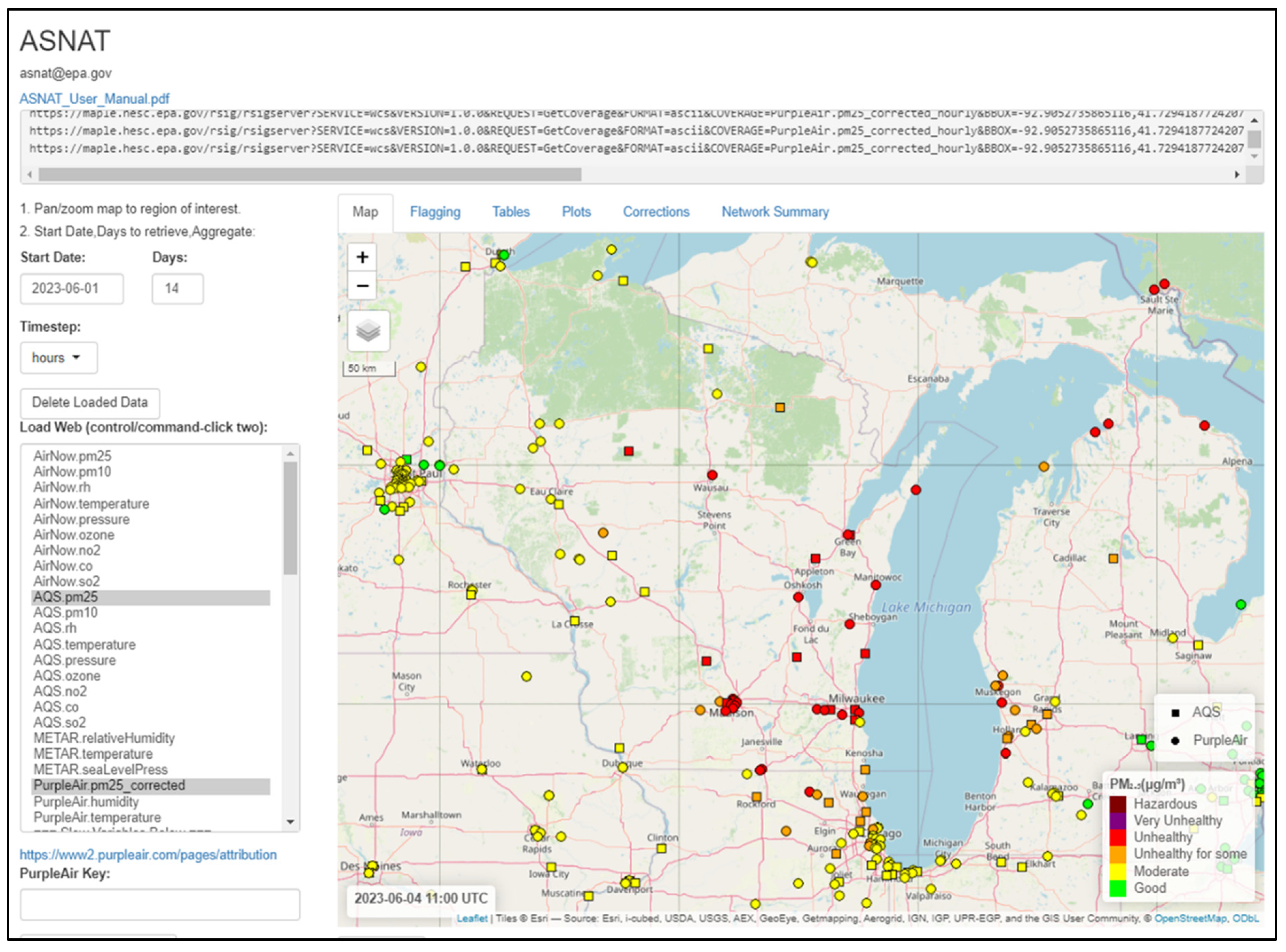
Figure 2.
Day of week, hour of day, month, and weekday plots comparing all AQS and PurpleAir monitors selected in Figure 1.
Figure 2.
Day of week, hour of day, month, and weekday plots comparing all AQS and PurpleAir monitors selected in Figure 1.
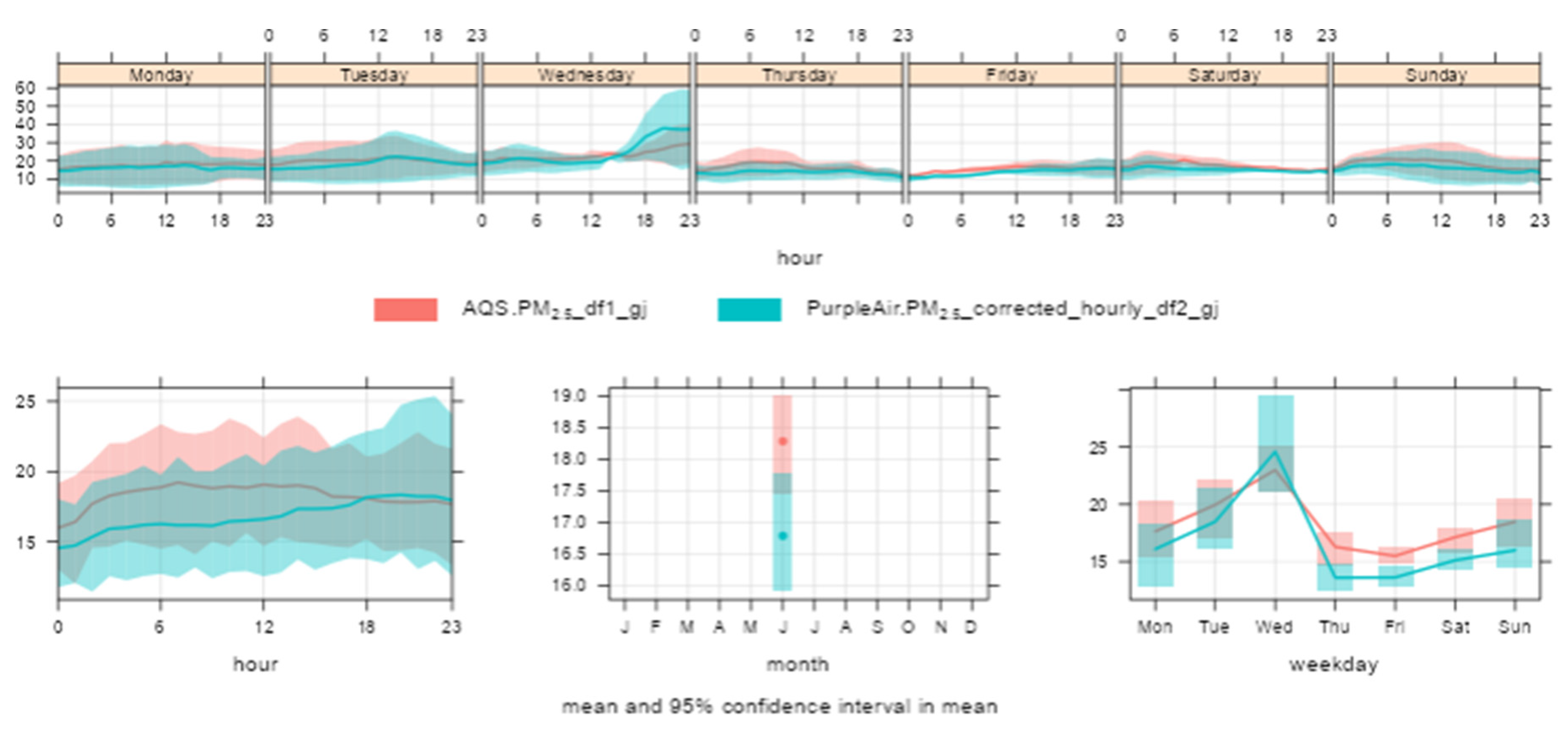
Figure 3.
Performance of PurpleAir sensors as compared to nearby monitors (data from AQS) for pairs within 250 meters at hourly averages. Black lines indicate the target range for each metric (coefficient of determination (R2), slope, intercept, root mean squared error (RMSE), and normalized root mean squared error (NRMSE)).
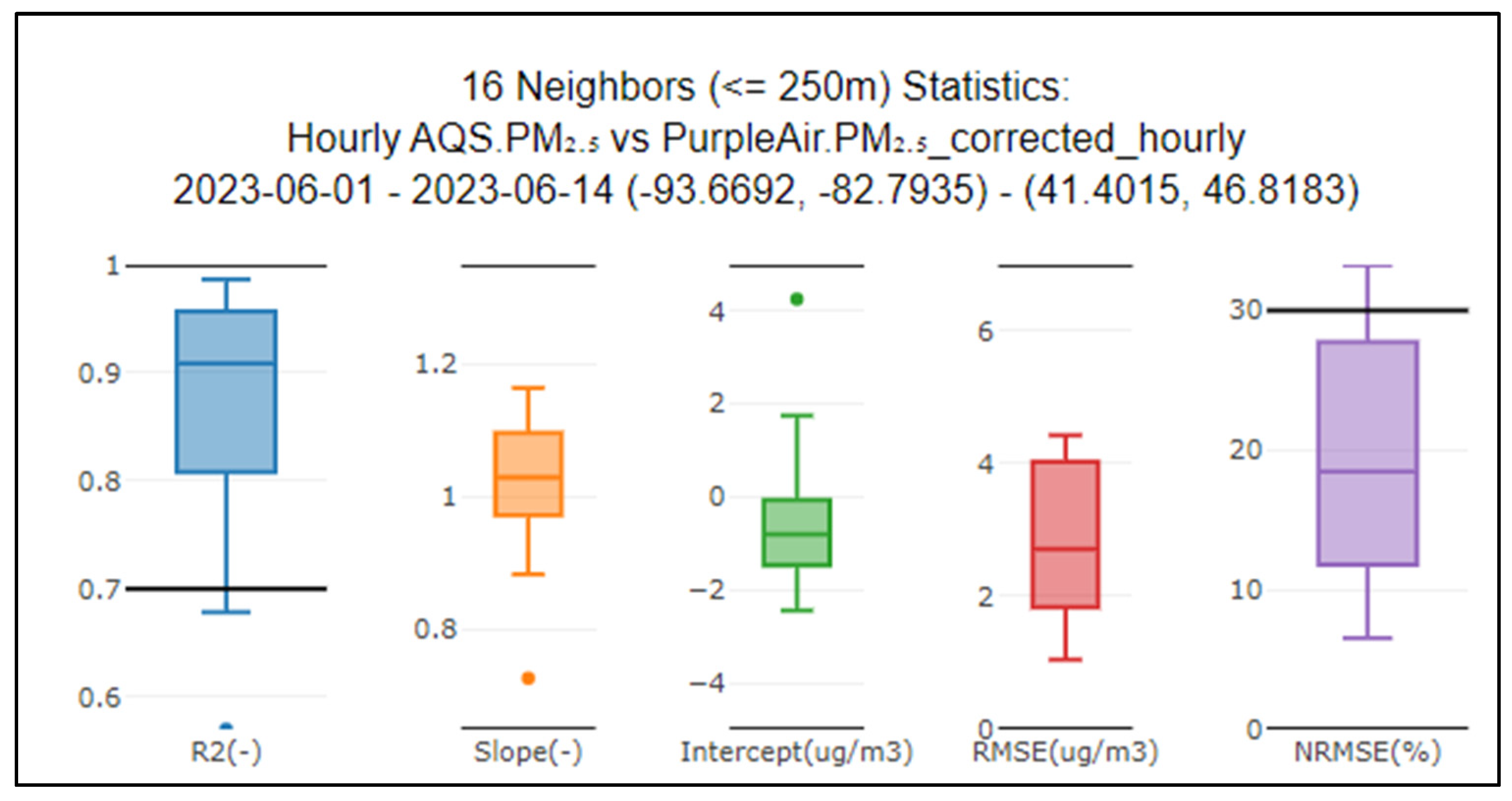
Figure 4.
Corrections generated for two example sensor-monitor pairs.
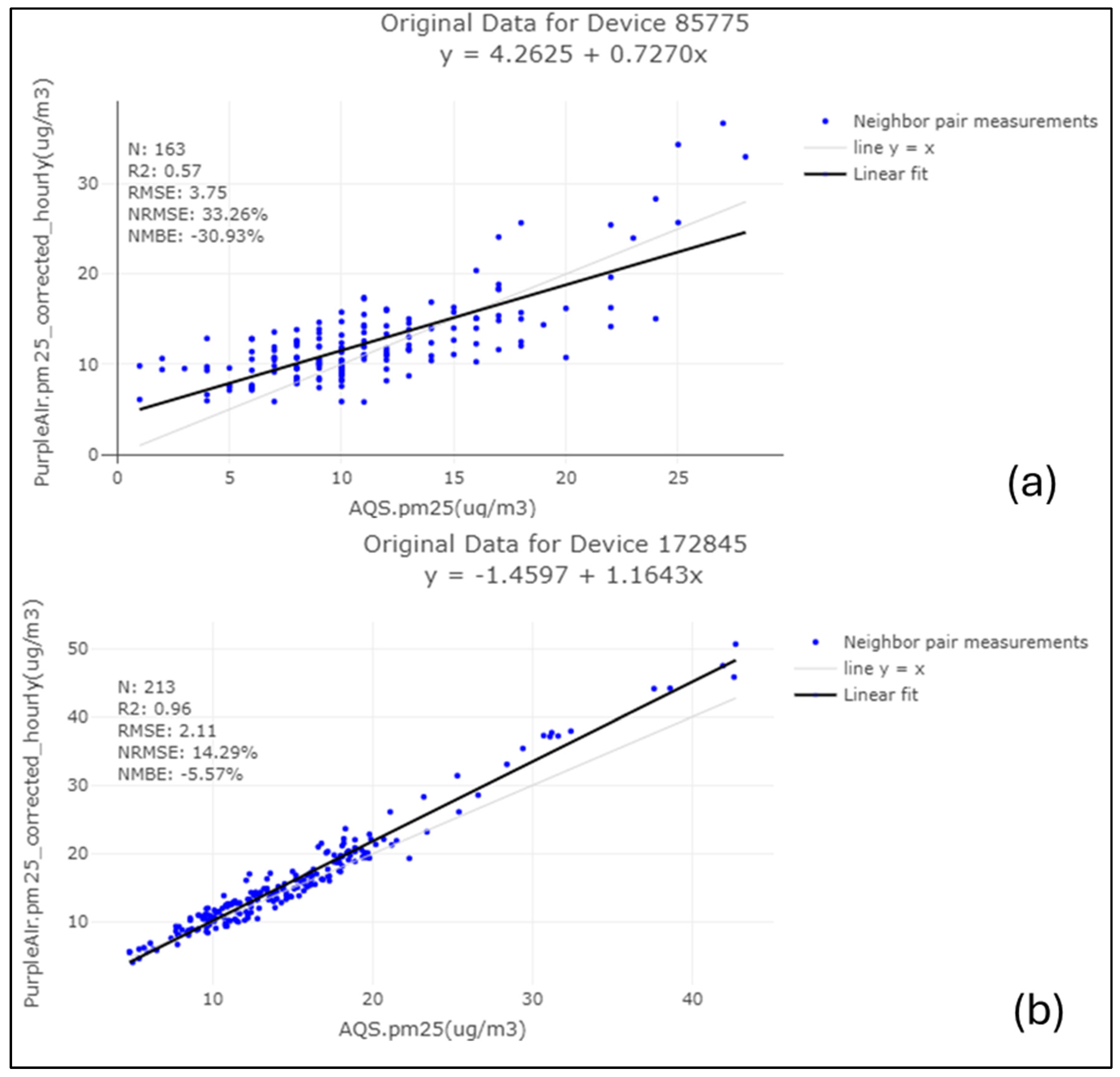
Figure 5.
Percentage of hourly PurpleAir PM2.5 measurements in each AQI category compared to the monitor (AQS) reported AQI category.
Figure 5.
Percentage of hourly PurpleAir PM2.5 measurements in each AQI category compared to the monitor (AQS) reported AQI category.
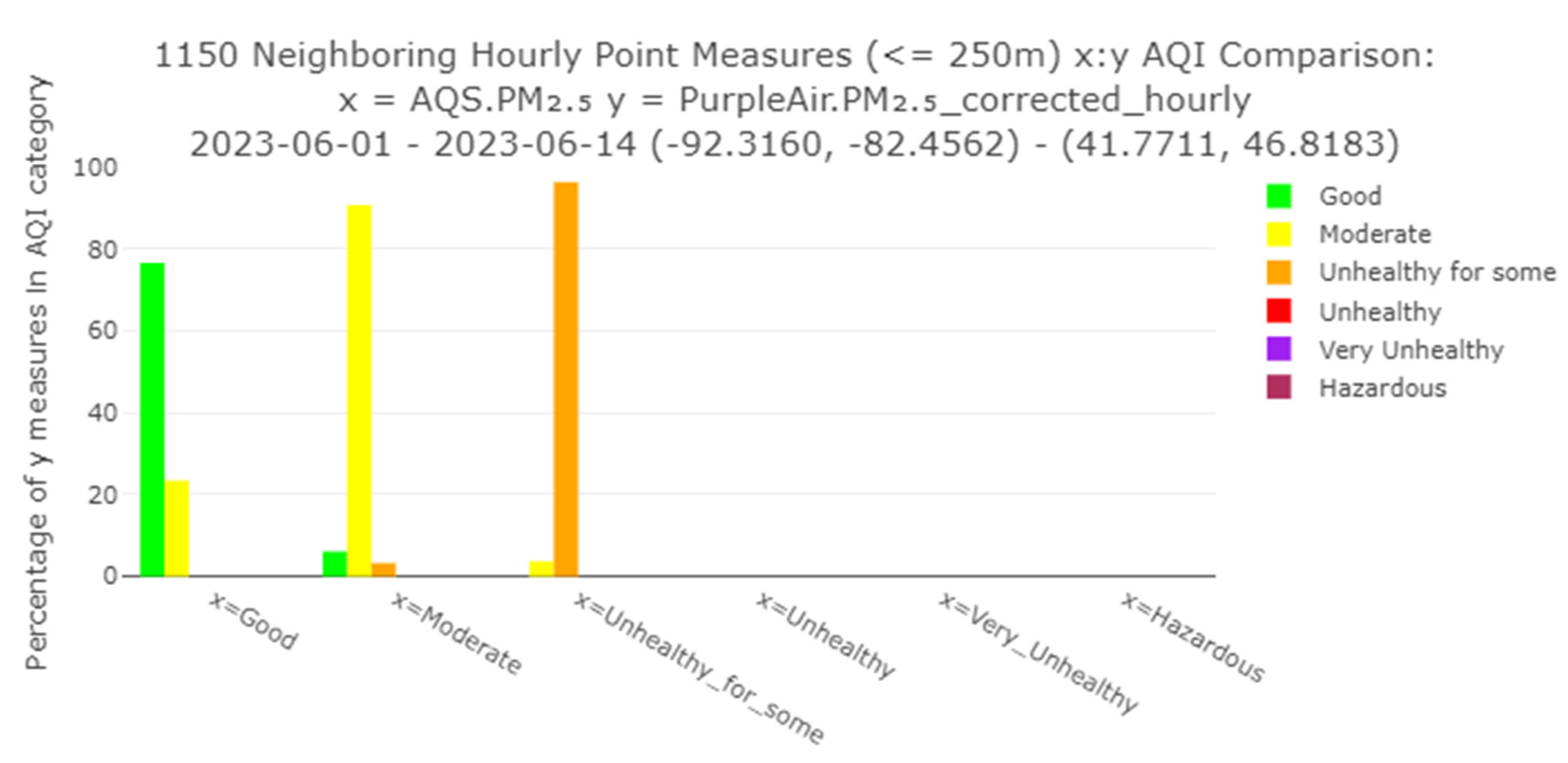
Figure 6.
ASNAT screenshot showing data flagging options/functionality.
Disclaimer/Publisher’s Note: The statements, opinions and data contained in all publications are solely those of the individual author(s) and contributor(s) and not of MDPI and/or the editor(s). MDPI and/or the editor(s) disclaim responsibility for any injury to people or property resulting from any ideas, methods, instructions or products referred to in the content. |
© 2025 by the authors. Licensee MDPI, Basel, Switzerland. This article is an open access article distributed under the terms and conditions of the Creative Commons Attribution (CC BY) license (http://creativecommons.org/licenses/by/4.0/).
Copyright: This open access article is published under a Creative Commons CC BY 4.0 license, which permit the free download, distribution, and reuse, provided that the author and preprint are cited in any reuse.


