
Submitted:
18 July 2025
Posted:
21 July 2025
You are already at the latest version
Abstract
Accurate estimation of traffic loads is critical for pavement and bridge design, among other transportation applications. Given the disproportional impact of heavier axle loads on pavement and bridge structures, truck and heavy vehicle traffic is expected to be a major determinant of traffic load estimation. Further, heavy vehicle traffic is also a major input in transportation planning and economic studies. The traditional method for estimating heavy vehicle traffic primarily relies on Annual Average Daily Traffic (AADT) estimation using Monthly Day of the Week (MDOW) adjustment factors as well as percent heavy vehicles observed using statewide data collection programs. The MDOW factors are developed using daily and seasonal (or monthly) variation patterns for total traffic, consisting predominantly of passenger cars and other smaller vehicles. Therefore, while using these factors may yield reasonable estimates for total traffic (AADT), such estimates may involve a great deal of approximation or inaccuracy when applied to heavy vehicle traffic. This research aims at assessing the discrepancy involved in estimating heavy vehicle traffic using MDOW adjustment factors for total traffic (conventional approach) along with three other methods. These methods include using MDOW adjustment factors for total trucks (class 5-13), combination-unit trucks (class 8-13), as well as adjustment factors for each vehicle class separately. Results clearly indicate that the conventional method was outperformed by the other three methods by a large margin. Further, using class-specific adjustment factors, which is the most detailed and data-intensive method, does not necessarily yield a more accurate estimation of heavy vehicle traffic.
Keywords:
traffic loads
; heavy vehicles
; truck traffic
; adjustment factors
; traffic data collection
1. Introduction
Accurate traffic load estimations are critical for the planning, design, and maintenance of transportation infrastructure. These estimates enable optimized maintenance schedules, efficient resource allocation, and optimal truck weight enforcement strategies, ultimately extending the lifespan of transportation infrastructure. Trucks and heavy vehicle traffic comprise a significant proportion of overall traffic loads, exerting a higher impact on infrastructure due to their higher weight and load intensity. Truck transportation is a vital component of freight transportation, substantially impacting state, regional, and national economies. In 2018, truck freight contributed around 40% of the overall U.S. ton-miles of freight, typically making 70% - 80% of total shipments and tonnage [1,2]. However, the continuous growth in truck traffic has a negative impact on highway networks, increasing crashes, congestion, and accelerated bridge and pavement degradation.
Over the last decade, there has been an increasing focus among practitioners and researchers on managing, monitoring, and planning freight transportation networks. The Moving Ahead for Progress in the 21st Century Act (MAP–21) established provisions intended to enhance freight movement requiring continual evaluation of the condition and performance of the U.S. freight network [3]. Therefore, most state highway agencies (departments of transportation (DOTs)) have established explicit plans for freight traffic to optimize statewide truck flow efficiency. The most critical data input supporting these plans is comprehensive truck volume information for the whole network [4].
2. Background
The estimation of truck volume has attracted significantly less focus than Annual Average Daily Traffic (AADT) estimation and has been relatively underexplored in the existing research. This section provides a brief overview of the heavy vehicle estimation in the current practice followed by a summary of the relevant studies in the existing literature.
Currently, many highway agencies use the conventional Monthly Day of the Week (MDOW) adjustment factors to estimate total and truck traffic, as reported in the FHWA Traffic Monitoring Guide [5]. The permanent traffic detector stations (Automatic Traffic Recorders (ATRs) and Weigh-In-Motion (WIM) stations) are used to develop daily and monthly variation patterns, in the form of Monthly Day of the Week (MDOW) adjustment factors, for various highway groupings (highways grouped by functional class and area type) [6]. These factors are then used with short-term counts in estimating the AADT and subsequently in estimating traffic loads throughout the network using observed heavy vehicle percentage. The MDOW factors represent the daily and seasonal (or monthly) variation patterns for total traffic, consisting predominantly of passenger cars and other smaller vehicles. The FHWA has emphasized predicting specific vehicle classes instead of total AADT using the temporal variation patterns for specific vehicle classes [7]. This results in the calculation of adjustment factors for each individual class (class 1 - 13). Using this approach, the adjustment factors from the individual classes are used with short-term counts by vehicle class to estimate each vehicle class individually and subsequently combining these estimates to find counts by vehicle category (e.g., total vehicles, total trucks, combination trucks, etc.). While this may seem labor-intensive and time-consuming, the use of traffic data management and analytics software has greatly facilitated the development of class-specific adjustment factors.
In the following paragraphs, the studies on estimating heavy vehicle traffic for operational analyses are summarized with major findings highlighted. It is important to note that forecasting heavy vehicle traffic for planning applications is less relevant to the research in hand, and as such only a brief discussion of those studies is provided.
A study conducted in New Jersey utilized the stepwise linear regression with a direct demand approach to determine the roadway and land use variables for truck volumes estimation [8]. The researchers collected count data for truck traffic from 270 locations across New Jersey and extracted data for land use within a one-mile buffer of individual highway segments. Key control variables included the number of businesses and employees and the estimated volume of sales. Regression models were established for various roadway types. The R-squared values for these models ranged from 0.35 - 0.97.
Another pertinent work investigated the use of full Bayesian negative binomial models and linear regression to estimate the annual average daily truck traffic (AADTT) of heavy-duty vehicles using data from 67 continuous count sites in Ohio [7]. The ADTT (average daily traffic for heavy-duty trucks), FC (functional class), population density, state-specific count station locations, and day of the week were important explanatory factors. Model development requires at least a continuous 24-hour collecting period at study locations.
Ports are one of the major truck trip generators. In a study, two kernel-based machine learning models (Gaussian Processes (GPs) and ε-Support Vector Machines (ε-SVMs)) have been applied to predict truck traffic at seaport terminals, using terminal operation data from the Port of Houston [9]. The study investigated import and export truck trips separately and compared the performance with a multilayer feedforward neural network (MLFNN). The results showed a comparable performance of these two machine learning models with the MLFNN, while requiring less effort in model fitting making them more effective alternatives for truck traffic estimation at seaports.
Linear optimization techniques have also been used in truck volume estimation. In a recent study, linear optimization has been utilized to estimate large trucks (LT) volume by utilizing volume and occupancy data from loop detectors [10]. This approach dynamically adjusts the vehicle lengths to accommodate varying traffic conditions and speeds, providing accurate LT estimation in both real-world and simulated scenarios when compared to ground truth data from weigh-in-motion (WIM) stations and videos.
Recently, several transportation agencies have started using probe vehicle data to monitor and assess the operation of transportation systems. A survey of planning and operation officials from fourteen highway agencies in the United States showed that the most desirable output from the probe data, other than total traffic volume, was the volume or percentage of heavy truck traffic [11]. Another study tested the application of probe data from short-term traffic counts for estimation of AADT by type of vehicle by creating models with multiple predictors [12]. Many states have started to utilize the National Performance Management Research Data Set (NPMRDS), which is provided by the FHWA and mandated by the requirements of MAP-21. A couple of studies [13,14] reported a robust correlation between probe vehicle counts on the one hand and overall traffic volumes and truck volumes on the other hand. Another recent research presented a machine learning-based model for estimating truck volumes at a state level using truck probe data in Kentucky [15]. In this research, annual average daily truck probe (AADTP) was developed as a metric, showing a strong correlation with truck AADT. The random forest outperformed the other models, and the truck volume profile for the freight network in Kentucky was demonstrated as a model utility. In another recent study, the accuracy of AADT, heavy vehicle traffic, medium-duty truck traffic, and heavy-duty truck traffic volumes has been assessed using probe-based activity indices from a North American company called StreetLight Data (StL) [16]. The total traffic estimates had the lowest errors with Mean Absolute Percentage Errors (MAPEs) ranging from 8.8% to 22.1% while in the case of heavy-duty truck traffic, the estimates showed the highest errors with MAPEs ranging from 56.6% to 96.4%. Medium-duty trucks performed better with manually scaled indices, with MAPEs ranging from 20.6% to 52.2%.
In planning applications, a few researchers have focused on freight demand models, such as commodity flow-based models, vehicle trip-based models, and agent- and tour-based models that have never been applied to a state level [17]. Truck trips are managed in vehicle trip-based models in a manner that emulates how passenger demand models manage passenger trips [18]. Commercial traffic surveys are frequently required first to comprehend the behavior of truck drivers and afterwards construct attraction and trip generation models based on commodity groups and truck types. Subsequently, equations that have been adjusted to fit the data are employed to calculate the number of truck trips. These calculations are based on sociodemographic variables, including employment and population. During the trip distribution phase, the estimation of truck trips between each origin-destination (OD) pair is carried out utilizing spatial interaction models, such as the gravity model [19]. Since only trucks are considered, the mode split step is skipped, and the OD matrix is applied to the highway network. This is usually done by using Wardrop’s user equilibrium concept or by using an all-or-nothing assignment method to determine truck trips across the network [17]. Research was conducted in Washington state, where the method was modified by creating a logical model to predict the transportation of goods along the potato value chain [20]. The number of trucks required was calculated at each stage using the least cost function in ArcGIS. This resulted in the count of truck journeys that passed through each individual section of the road network. Researchers have employed two primary methods to create commodity flow-based models [17]. The first approach is comparable to vehicle trip-based models and entails initially performing commodity flow surveys or acquiring pre-existing commodity flow data from external sources. The data is utilized to develop commodity-specific production and consumption models through the application of an input-output or linear regression model [21,22]. The second, more often used method is a top-down approach that starts with aggregated data on the flow of commodities. These data are accessible at a larger geographic level [23,24]. The FHWA’s Freight Analysis Framework is the primary data source, containing integrated data from several sources. It offers information on freight movement by commodity type and transportation mode for 133 domestic and eight international regions. Due to the lack of sufficient detail in this data, it is common to apply disaggregation based on the proportionality assumption to produce zonal OD commodity-specific matrices for estimating freight demand and utilization in a statewide or regional model [24].
The literature review conducted in the course of this study confirmed that there is hardly any research that provides an investigation into heavy vehicle estimation using statewide traffic data collection programs and traffic adjustment factors, which are still being used as a primary source of truck volume estimation by most highway agencies.
3. Study Motivation
The MDOW factors are developed using daily and seasonal (or monthly) variation patterns for total traffic, predominantly passenger cars, and other smaller non-commercial vehicles. Therefore, while adjusting traffic counts using the MDOW factors may yield reasonable estimates for total traffic, such estimates may involve high inaccuracy when applied to heavy vehicle traffic. Specifically, it is well known that factors influencing the temporal variation in total traffic may not be relevant to the variation in commercial traffic over time, primarily dictated by freight movement on the highway network. For example, the summer personal travel season notably affects the seasonal variation in total traffic. However, it may not have any tangible effect on commercial traffic that is primarily driven by local and regional economies. Similarly, the annual growth of total traffic year after year (currently used for future traffic projection) may not echo that of commercial traffic that is driven by different demographic and economic factors. Based on the recent shift towards using specific vehicle class adjustment factors, there needs to be more research into the accuracy involved in estimating heavy vehicle traffic. The current research aims at assessing the accuracy (or inaccuracy) in estimating heavy vehicle traffic using MDOW adjustment factors for total traffic (conventional approach) along with other methods of using MDOW adjustment factors for specific classes or groups of heavy vehicle classes.
4. Study Approach
In order to investigate the level of accuracy involved in heavy vehicle traffic estimation, a group of WIMs/ATRs belonging to the same highway functional classification with a complete 365 days of traffic counts is required. Two highway functional classifications, “rural principal arterials – Interstate” and “rural principal arterials – Others,” were considered in this study as most of the freight movement takes place on these highways. Out of the stations selected in this study for each highway classification, one station was used for testing and validation (later known as the testing station), while the other stations were used for developing the traffic adjustment factors (later known as the training stations). The process was repeated multiple times, ensuring that each station was used as a testing station once while included in the training stations for all other iterations. Four different methods were used in developing MDOW adjustment factors: total traffic (class 1 – 13), total trucks (class 5 – 13), combination unit (CU) trucks (class 8 – 13), and separate vehicle class (separate MDOW adjustment factors for each class). For each iteration (i.e., a testing station and training stations), MDOW adjustment factors at the training stations were calculated using each of the four methods. For the testing station, daily volumes were treated as short-term counts. Using MDOW adjustment factors by a given method, the percent discrepancy (% approximation) was calculated for each day of the year. Finally, the average discrepancy in heavy vehicle traffic estimation at the testing station for each method was calculated over one full year. MDOW factors were calculated using the following equation:
5. Data Collection
Study data were acquired through the Montana Department of Transportation (MDT) traffic data collection program. As discussed earlier, this study required a full year of traffic data at ATR and WIM stations belonging to the same highway functional classification (MDOW factors are developed individually for each functional class). Given data availability and use of heavy vehicle traffic, only two functional classifications were considered in this study. Specifically, upon examining data availability from 2019 to 2023, it was decided to use the ATR/WIM data from 2021 for “Rural Principal Arterials – Interstate” and 2022 data for “Rural Principal Arterials – Others.” The former classification includes rural interstate highways while the latter classification includes major rural arterials, claiming most of the freight traffic in the state of Montana. The data collected was a complete year (365 days) of traffic volume for each vehicle class (class 1 – 13) at each station. Table 1 shows the available WIM/ATR data with the full year (365 days) of traffic count from the year 2019 through 2023 with the ones selected in this study highlighted in gray.
Figure 1 shows the location of the selected WIM and ATR stations selected in this study. The purple circled stations are “rural principal arterials – Others” sites, while the ones circled in red are “principal arterials – Interstate” sites. The WIM sites are labeled as “W” and ATR sites are labeled as “C”.
6. Analysis and Results
This section summarizes the results of the current study, which are presented and discussed separately for each of the four methods of MDOW adjustment factor development.
6.1. Method I (Base Condition - Total Traffic)
This is the conventional way of developing MDOW adjustment factors. This method utilizes the daily and seasonal (monthly) variation patterns for total traffic, consisting predominantly of passenger cars and other smaller non-commercial vehicles, in estimating heavy vehicle traffic (using AADT and other information such as % heavy vehicles). The procedure was followed as mentioned in the study approach. A rotating variable testing station approach was used for both functional classes. Figure 2 shows the percent discrepancy in estimating total trucks and CU trucks for the rural principal arterial – others (RPA-O) classification. A high level of approximation can clearly be seen both for the total and CU trucks. As discussed earlier, this may largely be due to the fact that the factors influencing temporal and seasonal variations in total traffic may not be very relevant to the variations in commercial traffic. Figure 3 also shows a similar trend of high discrepancies in total and CU trucks estimations for rural principal arterial – Interstate (RPA-I) classification. By examining the two figures, it’s clear that the discrepancy in heavy vehicle traffic estimation is more profound for RPA-O classification compared to the RPA-I classification. Further, while the total and CU trucks are associated with high discrepancy overall, those for CU trucks are slightly higher in most cases as shown in Figure 2 and Figure 3.
6.2. Method II (Using Total Trucks, Class 5-13)
In this method, instead of using total traffic, total trucks were used in deriving the adjustment factors for estimating heavy vehicle traffic. Figure 4 and Figure 5 show the average absolute percent discrepancy (AAPD) in total and CU trucks estimations for the two functional classifications discussed earlier. At a glance, both figures clearly show that the overall discrepancy in total and CU trucks estimations is lower for method II compared to those for method I (shown in Figure 2 and Figure 3). These results suggest that using the MDOW adjustment factors from total trucks instead of the total traffic improved the accuracy in heavy vehicle estimation as those factors better capture the temporal variation in truck traffic. Also, the CU trucks estimation is slightly higher than total trucks estimation in most cases. Again, the level of discrepancy associated with the RPA-O classification is greater than that for the RPA-I classification.
6.3. Method III (Using CU Trucks, Class 8-13)
This method utilizes the CU trucks only in calculating the MDOW factors at the training stations. The average absolute percent discrepancies in estimating total and CU trucks for the two functional classifications are shown in Figure 6 and Figure 7. Similar to method II, both figures clearly show a lower discrepancy for the total and CU truck estimations compared to method I. The range of discrepancy for both truck groups are roughly comparable to those shown in Figure 4 and Figure 5 using method II. Again, like the results from the previous methods, the discrepancy in CU trucks estimation is slightly higher than that for total trucks in most cases.
6.4. Method IV (Using Separate Vehicle Classes)
This was the most sophisticated method for calculating adjustment factors by considering each vehicle class separately. The FHWA has encouraged state highway agencies to calculate class-specific MDOW adjustment factors. The average absolute percent discrepancies in total and CU trucks estimation using method IV for the two highway classifications are shown in Figure 8 and Figure 9. Similar to methods II and III, the discrepancies in truck traffic estimations are notably lower than those shown in Figure 2 and Figure 3 for method I. However, in comparing method IV to methods II and III, it is clear that overall, method IV yielded slightly higher discrepancies for the RPA-O classification but slightly lower discrepancies for the RPA-I classification.
7. Comparison of Different Methods
Previous discussions focused on the discrepancy in heavy vehicle estimation using the four different methods independently. This section will focus on comparing the performance of the four methods regarding the accuracy of heavy vehicle estimation.
Figure 10a shows the average absolute percent discrepancy (AAPD) in total trucks estimation using the different estimation methods at the ten stations of the RPA-O classification. The figure clearly shows that Method I is consistently associated with much higher discrepancy in total truck estimation for nine out of the ten testing stations. Further, method I exhibited a trend that is much different from the other three methods. Methods II and III showed very similar trends and levels of discrepancy as the AAPD values are very close and comparable for most stations. Method IV exhibited an overall good performance in estimating heavy vehicle traffic, however, results suggest that it slightly lags behind methods II and III as it showed inferior performance at 6 out of 10 stations. Further, the trend shown for method 4 is slightly different from those for methods II and III.
Very similar trends are shown in Figure 10b for the estimation of the CU trucks at the same stations. Specifically, Method I was found to yield greater discrepancy in CU estimation at most stations. Methods II and III performed much better than the other two methods and their discrepancies at different stations were very close. Method IV, while showing much better performance compared to Method I, slightly lagged behind methods II and III. The relatively similar performance of methods II and III may largely be attributed to the fact that the vast majority of heavy vehicle traffic belongs to classes 8-13 which are part of the counts used in the two methods.
Figure 11a,b show the average absolute percent discrepancy in the estimation of total and CU trucks at the four stations with the RPA-I classification. These figures show very similar trends in regard to the performance of the four estimation methods. Specifically, unlike the other three methods, method I is associated with notably higher discrepancies in total and CU trucks estimation at the four stations. Methods II and III exhibited much better performance (compared to method I) with largely similar discrepancies at the four stations. Method IV also showed favorable performance comparable to methods II and III, however, the trend exhibited by method IV slightly deviates from those for methods II and III.
Figure 11.
Average absolute percent discrepancies (AAPDs) by four methods (for principal arterials – Interstate).
Figure 11.
Average absolute percent discrepancies (AAPDs) by four methods (for principal arterials – Interstate).
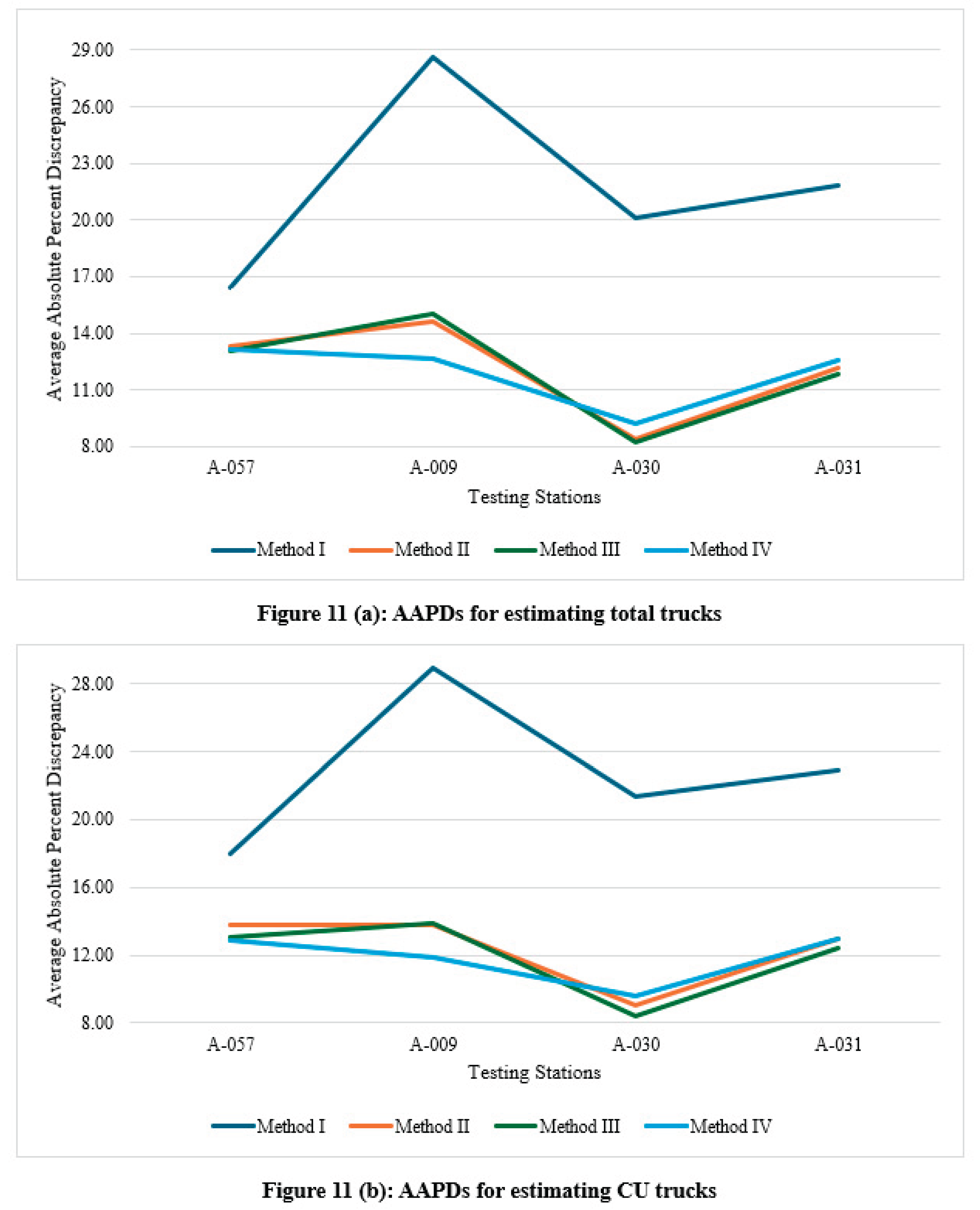
Table 2 shows the AAPDs and mean AAPDs for each method with the corresponding functional classification. In the case of RPA-O classification, the mean AAPD for method I is notably higher than that of the other methods. Further, methods II and II exhibited very similar performance as indicated by the very close mean AAPD values. Method IV, on the other hand showed a slightly higher mean AAPD, but it is still notably lower than method I. Compared to method I, there was a percentage decrease in mean AAPDs of 39.27%, 38.65% and 35.03% for method II, method III and method IV respectively for total trucks estimation. For CU trucks estimation, the corresponding percentage decrease in mean AAPDs compared to method I are 40.85%, 42.06% and 37.63% for methods II, III, and IV respectively.
In the case of RPA-I classification, method IV exhibited the lowest mean AAPD both for total and CU trucks estimation, followed by methods II and III which were only slightly higher in their mean AAPDs. Again, method I was associated with the highest mean AAPDs indicating higher discrepancy in heavy vehicle estimation. Compared to method I, there was a percentage decrease in mean AAPDs of 44.26%, 44.58% and 45.31% for methods II, III, and IV respectively for total trucks estimation. For CU trucks estimation, the corresponding percentage decrease in mean AAPDs were 45.59%, 47.52% and 48.09% for methods II, III, and IV respectively. In the case of RPA-O classification, method II provided better estimate for total trucks while method III provided better estimate for CU trucks. In the case of RPA-I classification, method IV provided better estimation for both total and CU trucks.
It is also of interest to see whether there is a statistical difference in the means of discrepancy between different methods in estimating total and CU trucks. For this, a two-tailed t-test was performed between the methods for all the testing stations using 95% confidence level. Table 3 shows the p-values from the t-test for testing the difference between different methods in the estimation of total and CU trucks for both highway classifications. Underlined values in red are for cases where the null hypothesis of the difference in discrepancy between methods is accepted.
The p-values, in comparing the means for total truck estimation between method I with the other three methods, were less than 0.001 (<0.001) at all testing stations for the RPA-O classification, showing a statistically significant difference between the means. The p-values for CU trucks estimation were less than 0.001 at all stations and comparisons, except one station in the comparison between method I and method IV. As the mean discrepancies in estimation for most of the testing stations were higher in method I compared to the other three methods, it was obvious that total traffic adjustment factors used in method I were performing poorly with high discrepancy in the estimation of total trucks and CU trucks. Similar results, in comparison between the means of method I with the rest of the three methods for RPA–I classification, can be seen in Table 3. The p-values were less than 0.001 at all testing stations, showing a statistically significant difference between the means while indicating the inferior performance of method I compared to the other methods. None of the cases in Table 3, show a statistically significant difference between the mean discrepancies of methods II and III at a confidence level of 95% indicating a similar performance of the two methods in estimating total and CU trucks. The p-values in comparing method IV with methods II and III showed that at a few stations, method IV estimates were very close to those of methods II and III, while the estimates were different at other stations.
8. Summary and Conclusions
An accurate estimation of commercial traffic and traffic loads is critical for pavement and bridge design, among other applications. Specifically, given the disproportional impact of heavier axle loads on pavement and bridge structures, truck and heavy vehicle traffic is expected to be a major determinant of traffic load estimation. The current practice in estimating AADT and traffic loads for various planning and design applications is outlined in the FHWA Traffic Monitoring Guide. The MDOW factors are developed using daily and seasonal (or monthly) variation patterns for total traffic, consisting predominantly of passenger cars and other smaller vehicles. Therefore, while adjusting traffic counts using the MDOW factors may yield reasonable estimates for total traffic, such estimates may involve a great deal of discrepancy when applied to heavy vehicle traffic. The current study aims to provide an investigation into the estimation of heavy vehicle traffic using the conventional MDOW factors (total traffic) as well as adjustment factors derived using three levels of aggregation: commercial traffic (class 5-13), CU trucks (class 8-13) and individual vehicle classes (i.e., class-specific MDOW factors). The major findings of the study are summarized below.
- i.
- Study results show that method I (traditional approach using total traffic adjustment factors) performed poorly in comparison with the other three methods consistently showing higher discrepancies. This finding is consistent with the fact that the factors affecting the temporal variations in total traffic may not be relevant to the variation in heavy vehicle traffic over time. The discrepancy in heavy vehicle traffic estimation is more profound for RPA-O classification compared to the RPA-I classification. This is somewhat expected given that much of the truck traffic on interstate highways is long-haul through traffic associated with more consistent daily and seasonal variation patterns.
- ii.
- Method II (total truck adjustment factors) and Method III (CU truck adjustment factors) estimated the heavy vehicle traffic with lower discrepancy, and the mean discrepancies at testing stations for both methods were very close. The similar performance of the two methods can be attributed to the fact that trucks in classes 5-7 only constitute a small proportion of trucks at most stations.
- iii.
- Method IV (no aggregation – class-specific adjustment factors) exhibited good performance overall compared to the other methods. However, this method did not exhibit better performance compared to method II or method III. Specifically, the method lagged behind methods II and III for the RPA-O classification (ten testing stations) while it was slightly better than methods II and III for the RPA-I classification (four testing stations). These results suggest that the class-specific adjustment factors (method IV), while more data-intensive and complicated, don’t necessarily yield more accurate estimates for total or CU truck traffic. This finding may be related to the small number of trucks (small sample size) in certain classes which may affect the accuracy of the MDOW factors for those classes.
While the current study provided valuable insights into the effectiveness of different ways of estimating heavy vehicle traffic, it was based on traffic data exclusive to the state of Montana. As heavy vehicle traffic patterns may vary by state and region, the authors recommend further research on heavy vehicle estimation using data from other states and geographic regions.
Author Contributions
The authors confirm contribution to the paper as follows: study conception and design: A.A.-K.; data collection: M.F.R.Q.; analysis and interpretation of results: M.F.R.Q. and A.A.-K.; draft manuscript preparation: M.F.R.Q. and A.A.-K. All authors reviewed the results and approved the final version of the manuscript.
Funding
This research received no external funding.
Data Availability Statement
The raw data supporting the conclusions of this article will be made available by the authors on request.
Acknowledgments
The authors would like to thank Peder Jerstad of the Montana Department of Transportation (MDT) for his help in traffic data collection for this research.
Conflicts of Interest
The authors declare no conflicts of interest.
Abbreviations
The following abbreviations are used in this manuscript:
| MDOW | Monthly Day of the Week |
| MDT | Montana Department of Transportation |
| FHWA | Federal Highway Administration |
| ATR | Automatic Traffic Recorder |
| AAPD | Average Absolute Percent Discrepancy |
References
- Shen G, Zhou L, Aydin SG. A multi-level spatial-temporal model for freight movement: The case of manufactured goods flows on the U.S. highway networks. Journal of Transport Geography. 2020; 88:102868. Available from: https://www.sciencedirect.com/science/article/pii/S0966692320309455.
- Bureau of Transportation Statistics. U.S. Ton-Miles of Freight. Available from: https://www.bts.gov/content/us-ton-miles-freight.
- Federal Highway Administration. MAP-21 - Moving Ahead for Progress in the 21st Century. Available from: https://www.fhwa.dot.gov/map21/factsheets/freight.cfm.
- Cohen H, Horowitz A, Pendyala R. National Cooperative Highway Research Program (NCHRP) Report 606: Forecasting Statewide Freight Toolkit. Washington, D.C.; Available from: www.TRB.org.
- Federal Highway Administration (FHWA). Traffic Monitoring Guide. 2022. Available from: https://rosap.ntl.bts.gov/view/dot/74643.
- Stephens J, Al-Kaisy AF, Villwock-Witte N, McCarthy D, Qi Y, Veneziano DA, et al. Montana Weigh-in-Motion (WIM) and Automatic Traffic Recorder (ATR) Strategy. 2017. Available from: https://rosap.ntl.bts.gov/view/dot/32517/dot_32517_DS1.pdf.
- Tsapakis I, Schneider IV WH, Nichols AP. A Bayesian analysis of the effect of estimating annual average daily traffic for heavy-duty trucks using training and validation datasets. Transportation Planning and Technology. 2013 Mar 1;36(2):201–17. Available from: . [CrossRef]
- Spasovic L, Ozbay K, Mittal N, Golias M. Estimation of Truck Volumes and Flows. In 2004. Available from: https://api.semanticscholar.org/CorpusID:106467251.
- Yuanchang X, Nathan H. Kernel-Based Machine Learning Models for Predicting Daily Truck Volume at Seaport Terminals. Journal of Transportation Engineering. 2010 Dec 1;136(12):1145–52. Available from: . [CrossRef]
- Gu Y, Liu D, Stanford J, Han LD. Innovative Method for Estimating Large Truck Volume Using Aggregate Volume and Occupancy Data Incorporating Empirical Knowledge into Linear Programming. Transportation Research Record: Journal of the Transportation Research Board. 2022 Jun 9;2676(11):648–63. Available from: . [CrossRef]
- Hou Y, Young SE, Sadabadi K, SekuBa P, Markow D. Estimating Highway Volumes Using Vehicle Probe Data - Proof of Concept: Preprint. In: ITS World Congress. Montreal; 2017. Available from: https://www.osti.gov/biblio/1426856.
- Schewel L, Co S, Willoughby C, Yan L, Clarke N, Wergin J. Non-Traditional Methods to Obtain Annual Average Daily Traffic (AADT). 2021. Available from: https://rosap.ntl.bts.gov/view/dot/64897/dot_64897_DS1.pdf.
- Zhang X, Chen M. Enhancing Statewide Annual Average Daily Traffic Estimation with Ubiquitous Probe Vehicle Data. Transportation Research Record. 2020 Jun 21;2674(9):649–60. Available from: . [CrossRef]
- Grande G, Lesniak M, Tardif LP, Regehr JD. Exploring vehicle probe data as a resource to enhance network-wide traffic volume estimates. Canadian Journal of Civil Engineering. 2021 Jun 23;49(4):558–68. Available from: . [CrossRef]
- Zhang X, Chen M. Statewide Truck Volume Estimation Using Probe Vehicle Data and Machine Learning. Transportation Research Record. 2023 Mar 27;2677(8):588–601. Available from: . [CrossRef]
- Zrobek C, Grande G, Regehr J, Mehran B. Evaluating the Accuracy of Probe-Based Truck Volumes using Continuous and Short-Duration Traffic Counts. Transportation Research Record. 2024 Apr 23;03611981241242070. Available from: . [CrossRef]
- Southworth F. Freight Flow Modeling in the United States. Appl Spat Anal Policy. 2018;11(4):669–91. Available from: . [CrossRef]
- Holguín-Veras J, List GF, Meyburg AH, Ozbay K, Teng H, Yahalom SZ. AN ASSESSMENT OF METHODOLOGICAL ALTERNATIVES FOR A REGIONAL FREIGHT MODEL IN THE NYMTC REGION. In 2001. Available from: https://api.semanticscholar.org/CorpusID:106903687.
- Dynamic Data Fusion Mining Private Sector Relationships and Public Databases to Enhance and Predict Freight Movement BACKGROUND AND CHALLENGE.
- Andreoli D, Goodchild A, Jessup E. Estimating truck trips with product specific data: a disruption case study in Washington potatoes. Transportation Letters. 2012 Jul 1;4(3):153–66. Available from: . [CrossRef]
- Proussaloglou K, Popuri Y, Tempesta D, Kasturirangan K, Cipra D. Wisconsin Passenger and Freight Statewide Model: Case Study in Statewide Model Validation. Transportation Research Record. 2007 Jan 1;2003(1):120–9. Available from: . [CrossRef]
- Souleyrette RR, Hans ZN. Statewide Transportation Planning Model and Methodology Development Program Final Report November 1996 Researchers. In 1996. Available from: https://api.semanticscholar.org/CorpusID:10125769.
- Shen G, Zhou L, Aydin SG. A multi-level spatial-temporal model for freight movement: The case of manufactured goods flows on the U.S. highway networks. Journal of Transport Geography. 2020; 88:102868. Available from: https://www.sciencedirect.com/science/article/pii/S0966692320309455.
- Vadali SR, Aldrete RM, Bujanda A. Financial Model to Assess Value Capture Potential of a Roadway Project. Transportation Research Record: Journal of the Transportation Research Board. 2009 Jan 1;2115(1):1–11. Available from: http://journals.sagepub.com/doi/10.3141/2115-01.
Figure 1.
Study area showing selected WIM and ATR stations.
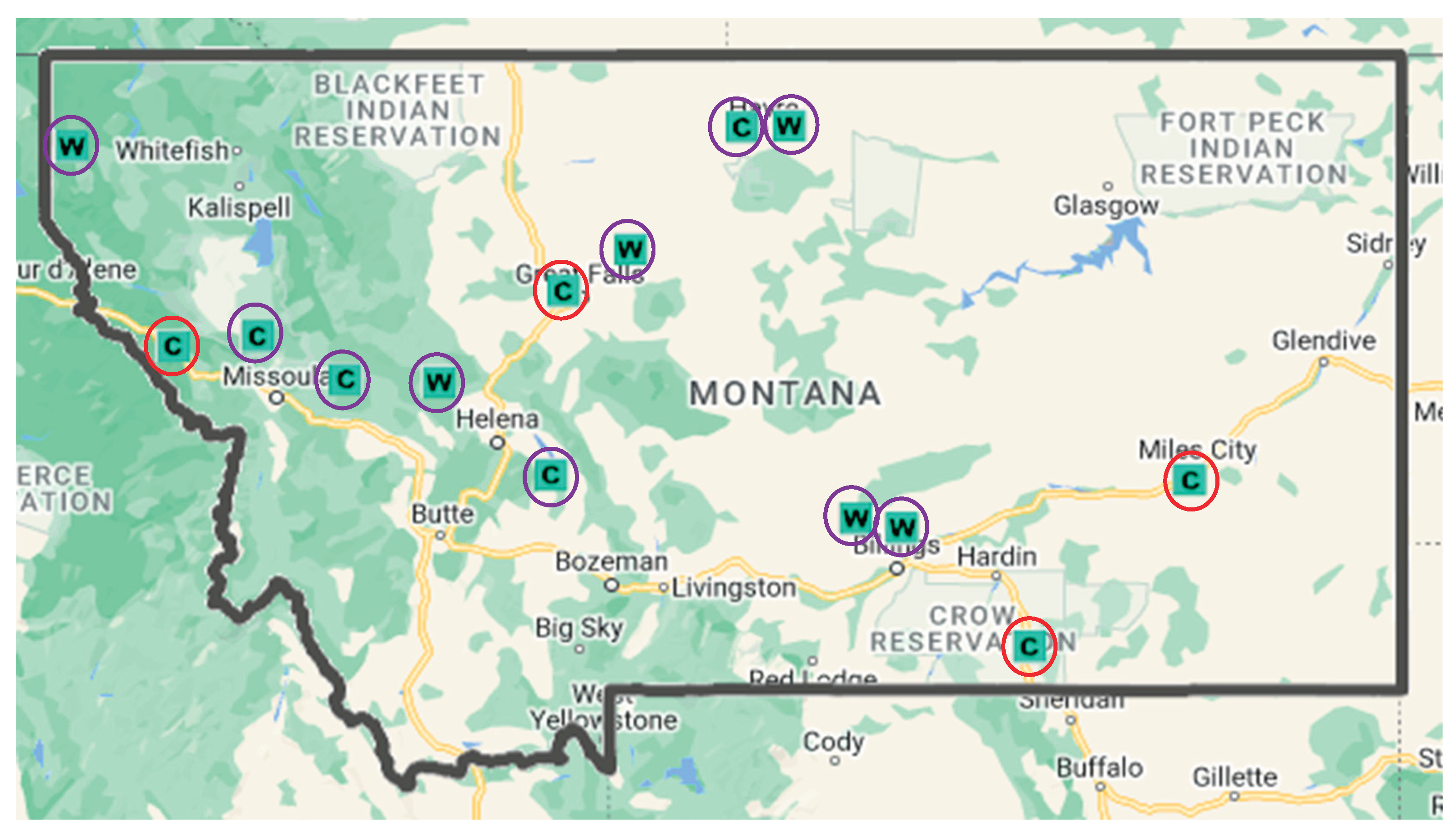
Figure 2.
Average absolute percent discrepancies for estimating total trucks and CU trucks (for rural principal arterials – others).
Figure 2.
Average absolute percent discrepancies for estimating total trucks and CU trucks (for rural principal arterials – others).
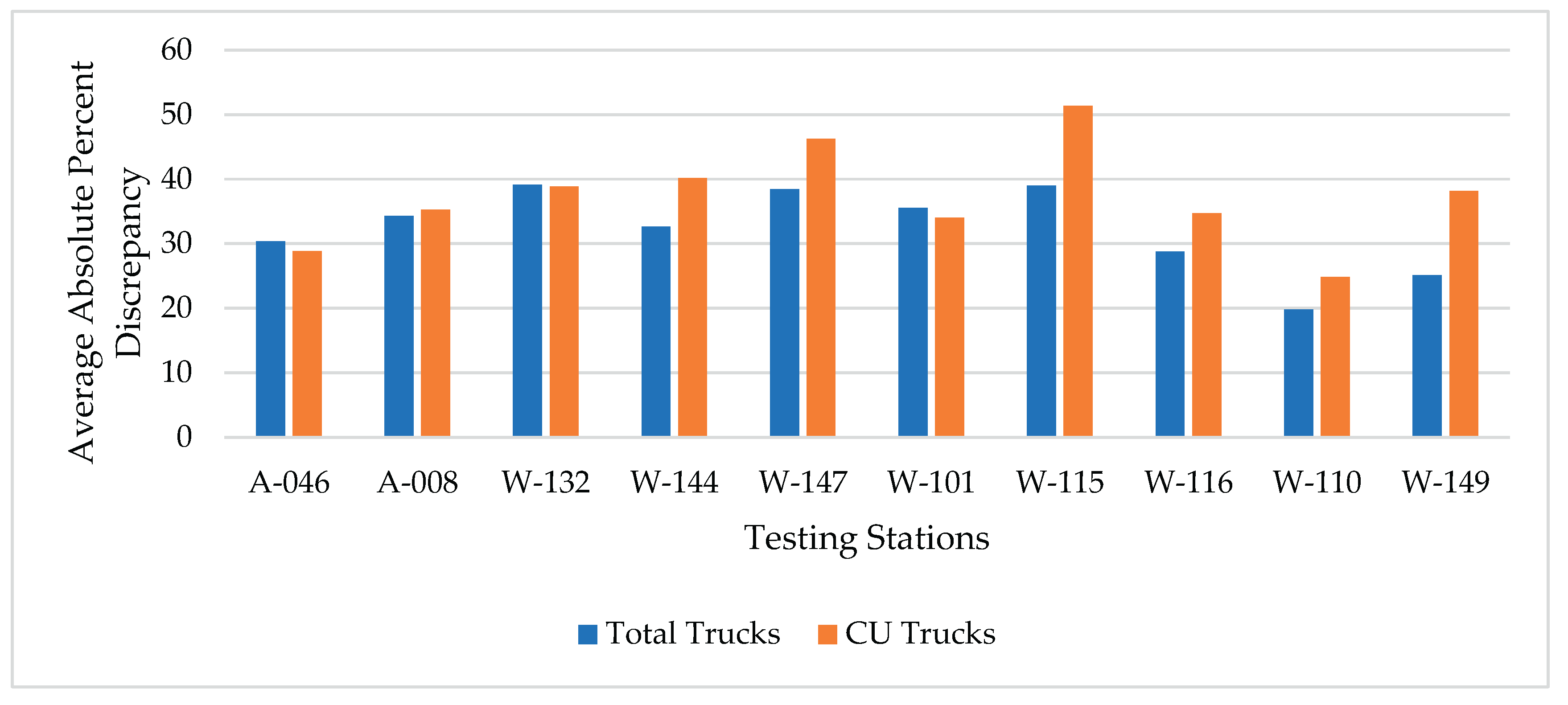
Figure 3.
Average absolute percent discrepancies for estimating total trucks and CU trucks (for principal arterials – interstate).
Figure 3.
Average absolute percent discrepancies for estimating total trucks and CU trucks (for principal arterials – interstate).
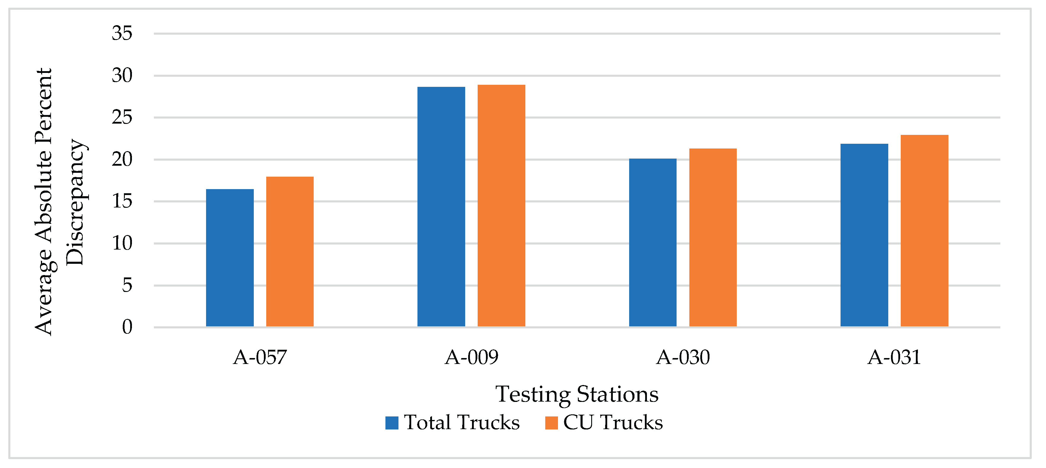
Figure 4.
Average absolute percent discrepancies for estimating total trucks and CU trucks (for rural principal arterials – Others).
Figure 4.
Average absolute percent discrepancies for estimating total trucks and CU trucks (for rural principal arterials – Others).
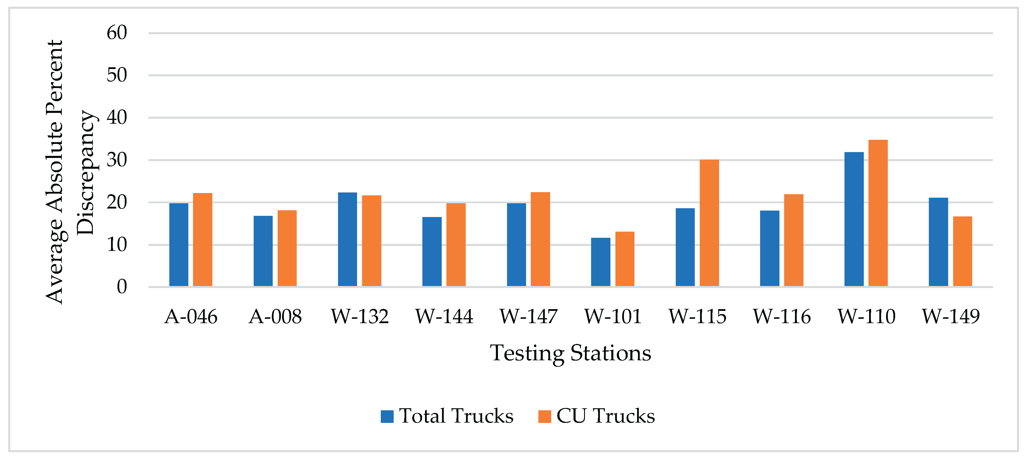
Figure 5.
Average absolute percent discrepancies for estimating total trucks and CU trucks (for principal arterials – Interstate).
Figure 5.
Average absolute percent discrepancies for estimating total trucks and CU trucks (for principal arterials – Interstate).
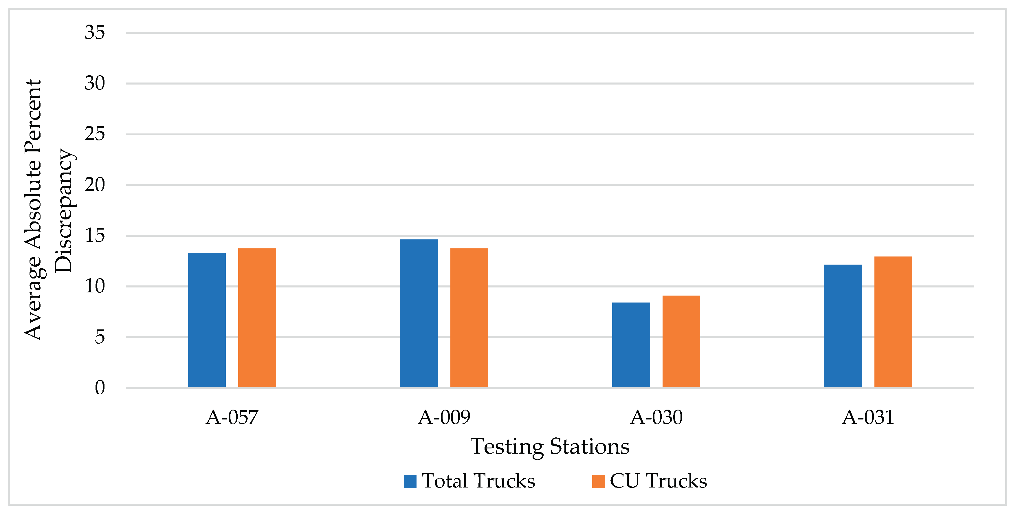
Figure 6.
Average absolute percent discrepancies for estimating total trucks and CU trucks (for rural principal arterials – Others).
Figure 6.
Average absolute percent discrepancies for estimating total trucks and CU trucks (for rural principal arterials – Others).
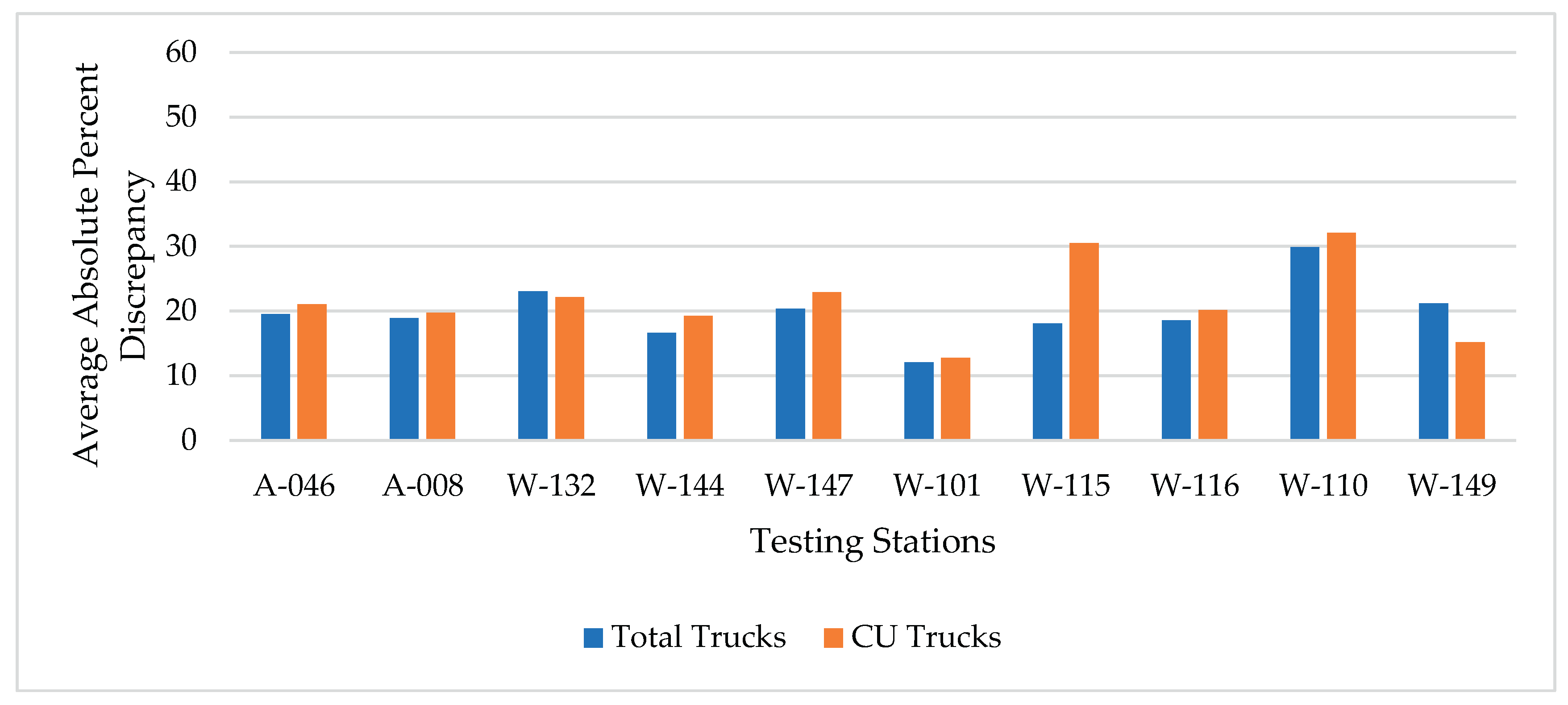
Figure 7.
Average absolute percent discrepancies for estimating total trucks and CU trucks (for principal arterials – Interstate).
Figure 7.
Average absolute percent discrepancies for estimating total trucks and CU trucks (for principal arterials – Interstate).
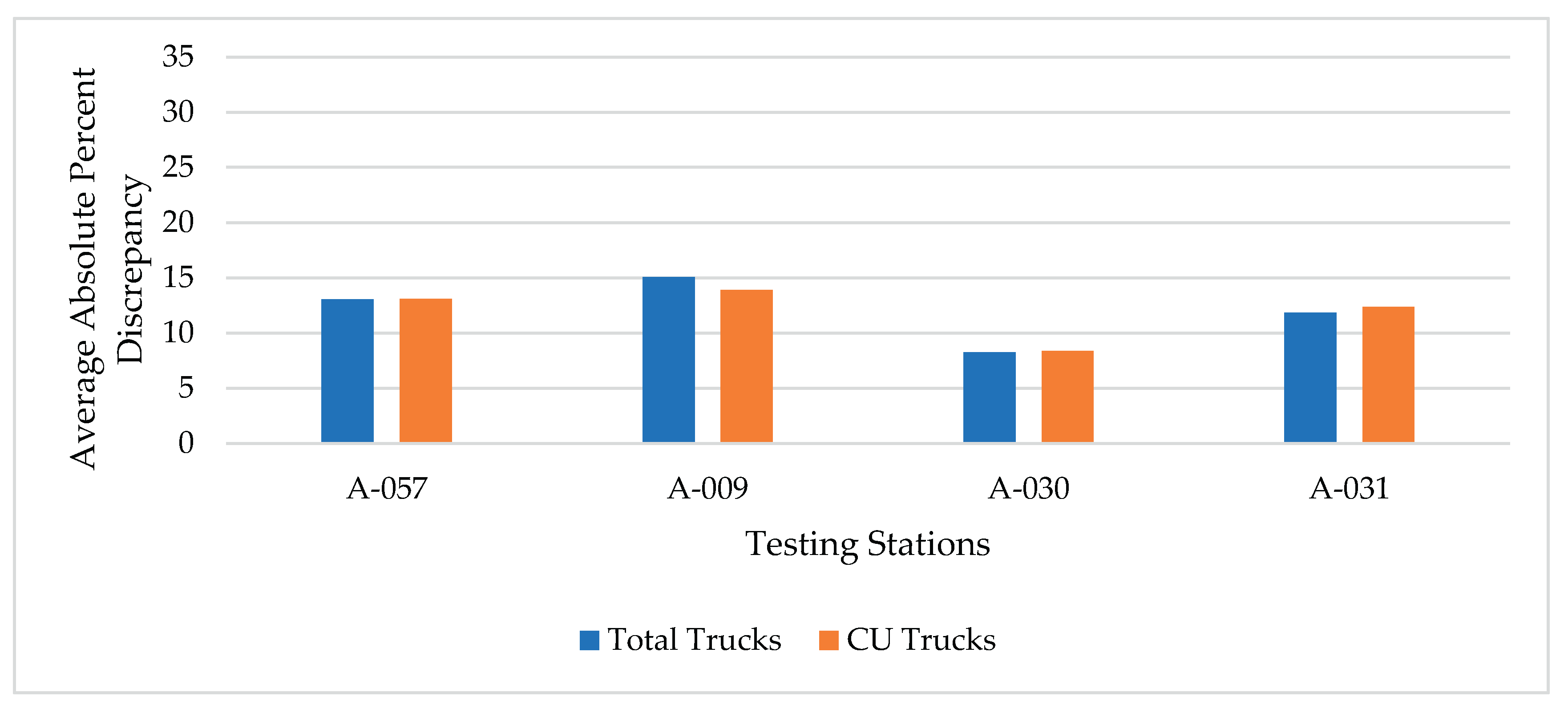
Figure 8.
Average absolute percent discrepancies for estimating total trucks and CU trucks (for rural principal arterials – Others).
Figure 8.
Average absolute percent discrepancies for estimating total trucks and CU trucks (for rural principal arterials – Others).
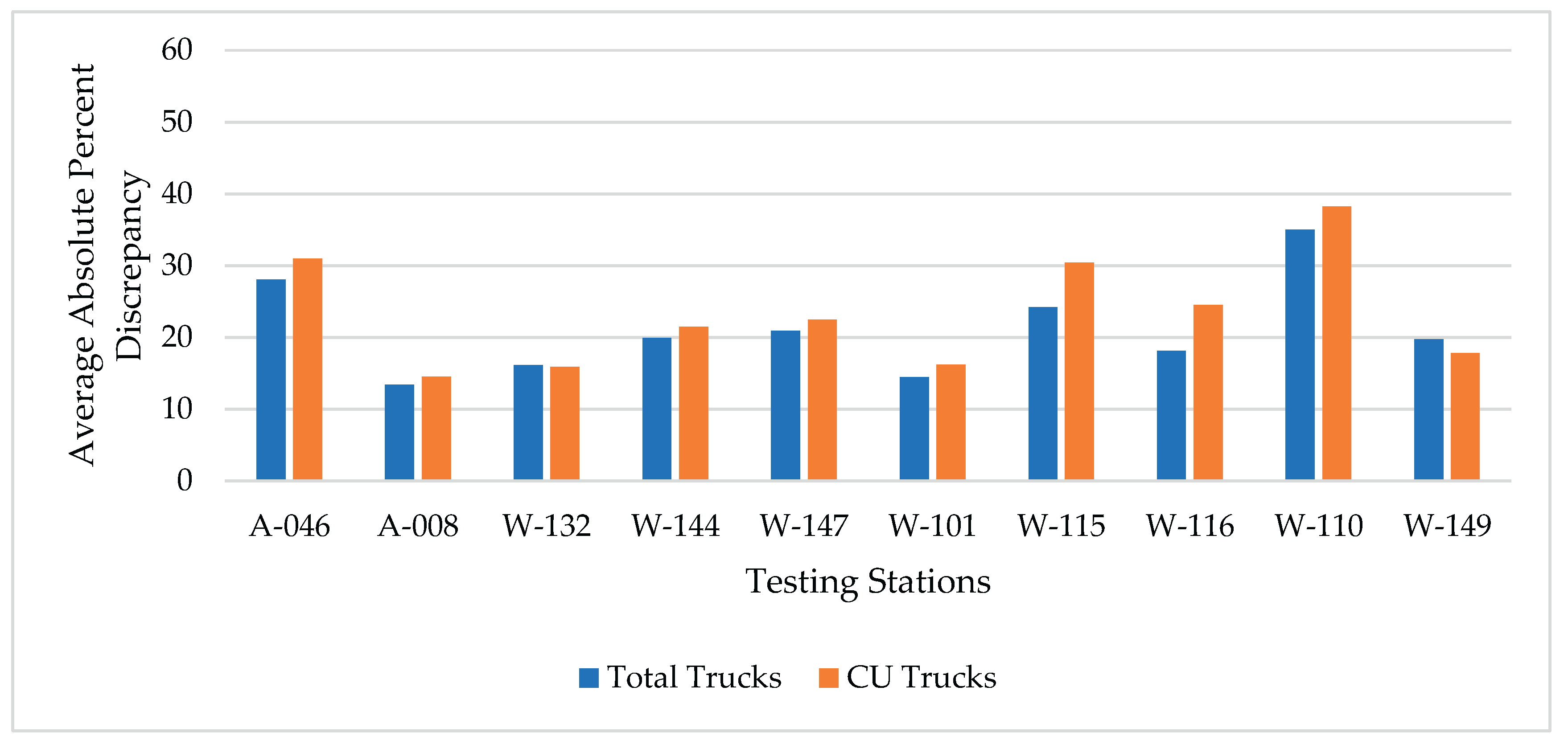
Figure 9.
Average absolute percent discrepancies for estimating total trucks and CU trucks (for principal arterials – Interstate).
Figure 9.
Average absolute percent discrepancies for estimating total trucks and CU trucks (for principal arterials – Interstate).
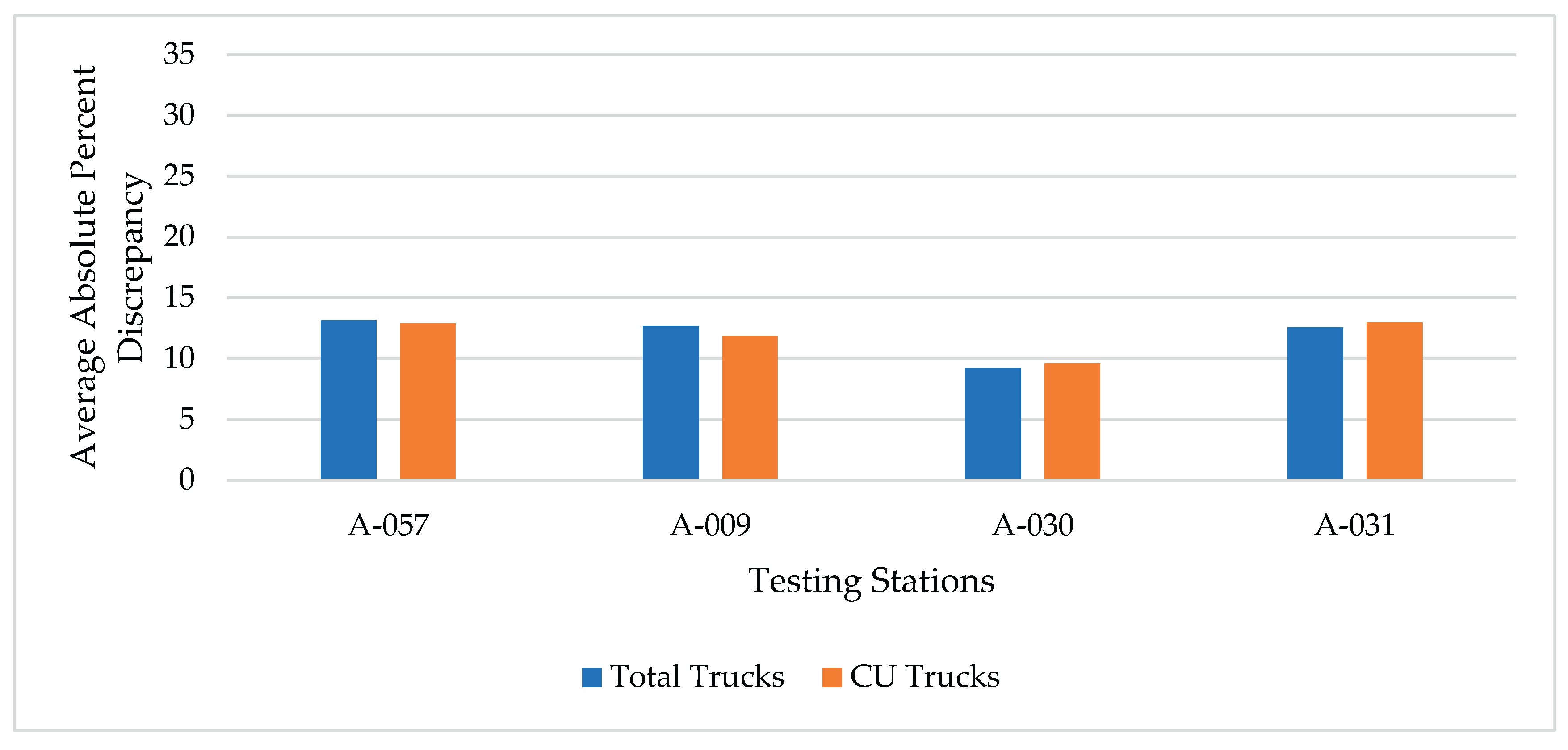
Figure 10.
Average absolute percent discrepancies (AAPDs) by four methods (for rural principal arterials – Others).
Figure 10.
Average absolute percent discrepancies (AAPDs) by four methods (for rural principal arterials – Others).


Table 1.
Available WIM/ATR data with full year (365 days) of traffic counts from 2019 to 2023.
| Functional Classes | Year | ||||
| 2019 | 2020 | 2021 | 2022 | 2023 | |
| Rural Principal Arterials – Others | 4 | 2 | 2 | 10 | 4 |
| Rural Principal Arterials – Interstate | 1 | 1 | 4 | 2 | 1 |
Table 2.
AAPD summary of each method and functional class. .
| Stations | Methods | |||
| Method I (Base) | Method II | Method III | Method IV | |
| Rural Principal Arterials – Others (RPA-O) | ||||
| A-008 | 34.34* [35.31] ** | 16.83 [18.16] | 18.94 [19.78] | 13.44 [14.53] |
| A-046 | 30.40 [28.89] | 19.75 [22.15] | 19.51 [21.08] | 28.10 [30.95] |
| W-132 | 39.19 [38.87] | 22.33 [21.60] | 23.07 [22.17] | 16.13 [15.88] |
| W-144 | 32.66 [40.22] | 16.56 [19.80] | 16.67 [19.28] | 19.94 [21.49] |
| W-147 | 38.51 [46.30] | 19.76 [22.36] | 20.35 [22.93] | 20.91 [22.46] |
| W-101 | 35.55 [34.05] | 11.62 [13.06] | 12.10 [12.76] | 14.45 [16.21] |
| W-110 | 19.82 [24.87] | 31.82 [34.77] | 29.92 [32.09] | 35.00 [38.24] |
| W-115 | 39.04 [51.37] | 18.62 [30.05] | 18.08 [30.50] | 24.24 [30.41] |
| W-116 | 28.78 [34.73] | 18.08 [21.90] | 18.59 [20.18] | 18.11 [24.54] |
| W-149 | 25.13 [38.16] | 21.10 [16.68] | 21.18 [15.18] | 19.75 [17.80] |
| Mean (RPA-O) | 32.34 [37.28] | 19.64 [22.05] | 19.84 [21.60] | 21.01 [23.25] |
| Rural Principal Arterials – Interstate (RPA-I) | ||||
| A-057 | 16.45 [17.94] | 13.32 [13.74] | 13.05 [13.09] | 13.13 [12.89] |
| A-009 | 28.64 [28.90] | 14.64 [13.76] | 15.06 [13.91] | 12.67 [11.85] |
| A-030 | 20.09 [21.31] | 8.41 [9.079] | 8.27 [8.40] | 9.23 [9.59] |
| A-031 | 21.87 [22.94] | 12.15 [12.96] | 11.86 [12.39] | 12.57 [12.96] |
| Mean (RPA-I) | 21.76 [22.77] | 12.13 [12.39] | 12.06 [11.95] | 11.90 [11.82] |
* AAPD for estimation of total trucks. ** AAPD for estimation of CU trucks.
Table 3.
P-Values from T-test for testing the significant difference between different methods. .
| Stations | Comparison of Methods | |||||
| MethodI vs MethodII | MethodI vs MethodIII | MethodI vs MethodIV | MethodIIvs MethodIII | MethodIIvs MethodIV | MethodIIIvs MethodIV | |
| Rural Principal Arterials – Others (RPA-O) | ||||||
| A-008 | <0.001* <0.001** |
<0.001 <0.001 |
<0.001 0.2956 |
0.0334 0.4452 |
<0.001 <0.001 |
<0.001 <0.001 |
| A-046 | <0.001 <0.001 |
<0.001 <0.001 |
0.2007 <0.001 |
0.853 0.4381 |
<0.001 <0.001 |
<0.001 <0.001 |
| W-132 | <0.001 <0.001 |
<0.001 <0.001 |
<0.001 <0.001 |
0.5711 0.6651 |
<0.001 <0.001 |
<0.001 <0.001 |
| W-144 | <0.001 <0.001 |
<0.001 <0.001 |
<0.001 <0.001 |
0.9194 0.6376 |
0.0072 0.2151 |
0.0084 0.0987 |
| W-147 | <0.001 <0.001 |
<0.001 <0.001 |
<0.001 <0.001 |
0.6025 0.6647 |
0.328 0.9379 |
0.6368 0.7187 |
| W-101 | <0.001 <0.001 |
<0.001 <0.001 |
<0.001 <0.001 |
0.5528 0.2565 |
0.0023 0.0029 |
0.0135 <0.001 |
| W-110 | <0.001 <0.001 |
<0.001 <0.001 |
<0.001 <0.001 |
0.4615 0.3677 |
0.283 0.1375 |
0.0759 0.0169 |
| W-115 | <0.001 <0.001 |
<0.001 <0.001 |
<0.001 <0.001 |
0.6167 0.3313 |
<0.001 0.0132 |
<0.001 <0.001 |
| W-116 | <0.001 <0.001 |
<0.001 <0.001 |
<0.001 <0.001 |
0.6811 0.2179 |
0.978 0.0992 |
0.710 0.004 |
| W-149 | 0.0033 <0.001 |
0.0043 <0.001 |
<0.001 <0.001 |
0.9535 0.1295 |
0.3711 0.3109 |
0.3448 0.0147 |
| Rural Principal Arterials – Interstate (RPA-I) | ||||||
| A-057 | <0.001 <0.001 |
<0.001 <0.001 |
<0.001 <0.001 |
0.7576 0.4425 |
0.8282 0.3148 |
0.9262 0.8158 |
| A-009 | <0.001 <0.001 |
<0.001 <0.001 |
<0.001 <0.001 |
0.6267 0.3858 |
0.0169 <0.001 |
0.0042 0.0122 |
| A-030 | <0.001 <0.001 |
<0.001 <0.001 |
<0.001 <0.001 |
0.5711 0.9863 |
<0.001 0.0698 |
<0.001 0.6875 |
| A-031 | <0.001 <0.001 |
<0.001 <0.001 |
<0.001 <0.001 |
0.8190 0.4867 |
0.2040 0.9996 |
0.1335 0.5039 |
* P-Value for estimation of total trucks. ** P-Value for estimation of CU trucks.
Disclaimer/Publisher’s Note: The statements, opinions and data contained in all publications are solely those of the individual author(s) and contributor(s) and not of MDPI and/or the editor(s). MDPI and/or the editor(s) disclaim responsibility for any injury to people or property resulting from any ideas, methods, instructions or products referred to in the content. |
© 2025 by the authors. Licensee MDPI, Basel, Switzerland. This article is an open access article distributed under the terms and conditions of the Creative Commons Attribution (CC BY) license (http://creativecommons.org/licenses/by/4.0/).
Copyright: This open access article is published under a Creative Commons CC BY 4.0 license, which permit the free download, distribution, and reuse, provided that the author and preprint are cited in any reuse.


