Submitted:
18 July 2025
Posted:
21 July 2025
You are already at the latest version
Abstract
Agricultural drainage canals provide critical habitats for fish species whose populations are sensitive to agricultural practices, highlighting the need for effective and non-invasive monitoring techniques. In this study, we developed a practical method using the YOLOv8n deep learning model to automatically detect and quantify fish occurrence in underwater images captured from an agricultural canal in Ibaraki Prefecture, Japan. Two fish species, Pseudorasbora parva (topmouth gudgeon) and Cyprinus carpio (common carp), which represent small- and large-bodied fish, respectively, were targeted. The trained YOLOv8n model achieved a high validation performance (F1-score = 91.6%, Precision = 95.1%, Recall = 88.4%), although external inference testing on 12,600 images indicated a reduced performance under practical field conditions (F1-score = 61.6%, Precision = 88.9%, Recall = 47.1%). By correcting for detection errors and repeated detections, we estimated that approximately 7,300 individuals of P. parva and 80 individuals of C. carpio passed the observation point over a seven-hour monitoring period. This study demonstrates the potential of deep-learning-based automated monitoring methods for sustainable aquatic ecosystem management in agricultural landscapes. Future research should focus on improving the detection Recall under challenging environmental conditions, such as turbidity and partial visibility, to enhance practical applicability.
Keywords:
deep learning
; YOLOv8
; object detection
; agricultural canal
; fish habitat
; non-invasive monitoring
; aquatic biodiversity
1. Introduction
Agricultural drainage canals serve as fish habitats that are strongly influenced by farming activities, and their conservation is essential to achieve sustainable agriculture that maintains biodiversity. In Japan, drainage canals are often significantly affected by irrigation and rural development projects, which frequently expose fish populations to abrupt habitat changes. For example, to lower groundwater levels in fields, facilitate the use of large machinery, and improve water conveyance in drainage canals, canal beds are often excavated deeper and lined with concrete. However, these interventions can increase flow velocity and reduce flow diversity, resulting in a decline in fish species diversity and population size.
Although the adoption of smart agriculture remains limited, it is expected to advance, potentially leading to substantial changes in water management practices. This may alter the flow conditions in the drainage canals. In Japan, eco-friendly fish habitat structures, such as artificial fish shelters (so-called “fish nests”) and fish refuges (“fish pools”), have been introduced into agricultural canals to enhance aquatic biodiversity [1]. However, methods for quantitatively evaluating the effectiveness of these structures are yet to be established. Thus, there is a need to develop approaches for sustainable canal renovation and to improve the performance of eco-friendly structures in ways that conserve aquatic ecosystems while maintaining agricultural productivity. Advancing these efforts requires a fundamental understanding of fish occurrence in drainage canals, underscoring the need for noninvasive and automated monitoring techniques. It is particularly important to estimate the number of fish species and individuals by using practical methods to ensure speed and accuracy.
When aiming to conserve fish populations in agricultural drainage canals, understanding the spatiotemporal distribution of resident fish is critical but often challenging. Direct capture methods have low catch rates, and tracking the behavior of small fish using tags poses several difficulties. Although recent attempts have been made to estimate fish species composition and abundance using environmental DNA (eDNA) [2], this approach has not yet allowed the estimation of the number of individual fish inhabiting specific sites.
Methods that input images into deep learning-based object detection models to rapidly detect fish in the ocean [3,4,5,6,7], ponds [8], rivers [9], and canals [10] have also been explored. Additionally, experiments have been conducted to improve fish detection accuracy in tank environments, primarily for aquaculture applications [11]. These approaches are direct and non-invasive, offering promising avenues for studying the temporal distribution of fish at specific sites. Because these methods primarily require underwater images as key data, they also have the advantage of low human and financial costs, making them suitable for the continuous monitoring of fish populations. However, agricultural drainage canals present many challenges for fish detection from underwater images, such as turbidity, falling leaves and branches from the banks or upstream, and dead filamentous algae drifting along the canal bed. Despite these issues, this field has rarely been studied.
In this study, we focused on the unique conditions faced by fish-inhabiting agricultural drainage canals. Specifically, we employed deep learning to automatically detect two target species—Pseudorasbora parva (topmouth gudgeon, known as “Motsugo” in Japanese) and Cyprinus carpio (common carp, “Koi”)—from underwater images taken in fish refuges constructed within drainage canals in Ibaraki Prefecture, Japan. We then presented a method to estimate both the total number of target fish and the frequency distribution of their occurrence. For the deep learning model, we utilized YOLOv8n (Ultralytics YOLOv8.1.42), a widely used detection framework capable of rapid and accurate recognition. This approach aims to contribute to practical and cost-effective techniques for continuous, non-invasive monitoring of fish populations in agricultural canals, ultimately supporting the sustainable management of aquatic ecosystems and agricultural productivity.
2. Materials and Methods
2.1. Fish Detection Model and Performance Metrics
In this study, we used YOLOv8n, a YOLO series model [12] released in 2023, as the fish detection model. YOLOv8n is lightweight and operates in low-power or low-specification systems. It produces the normalized center coordinates (x, y), width, and height of each bounding box (BB), along with the class ID and confidence score of the detected objects. The model was trained by minimizing a composite loss function that combined the BB localization, classification, and confidence errors.
To evaluate the performance of this model, we used the Precision, Recall, F1-score, Average Precision (AP), and mean Average Precision (mAP), as defined by Eqs. (1)–(5): here, true positives (TPs) represent the number of correctly detected target objects, false positives (FPs) denote detections that do not correspond to actual objects, and false negatives (FNs) refer to actual objects missed by the model.
Precision (Eq. 1) reflects the proportion of correct detections among all detections, calculated as TP divided by the sum of TP and FP. Recall (Eq. 2) indicates the proportion of actual objects that are successfully detected, computed as TP divided by the sum of TP and FN. Because Precision and Recall typically have a tradeoff relationship, we also used the F1-score (Eq. 3), the harmonic means of the Precision and Recall, as a comprehensive metric.
To determine whether a detection was counted as a true positive, we used the intersection over union (IoU), defined as the area of overlap divided by the area of union between the predicted and ground truth BB. We calculated the AP for each class i, APi, in Eq. (4), as the area under the Precision–Recall curve, where Pi(r) denotes the Precision at a given Recall r. Finally, mAP (Eq. 5) was obtained by averaging the AP values across all N classes, thus integrating both the classification and localization performances to provide an overall indicator of detection accuracy.
The mAP reported here was specifically calculated by averaging AP values across IoU thresholds ranging from 0.50 to 0.95 in 0.05 increments, commonly referred to as mAP50–95.
2.2. Image Data
Underwater images were acquired from the main agricultural drainage canal (3 m wide) located in Miho Village, Ibaraki Prefecture, Japan. The fish refuge in this canal was constructed by excavating the entire canal bed to a depth of 0.5 m, although sedimentation has progressed in some areas. The average bed slope of the canal was 0.003. In this canal, sediment tends to accumulate within artificial fish shelters and fish refuges [13], and filamentous attached algae growing on the bed often detach and drift downstream, with some accumulating inside the shelter [14].
A time-lapse camera (TLC200Pro, Brinno) enclosed in waterproof housing was installed on the downstream side of an artificial fish shelter situated within the fish refuge on the right bank. Figure 1 shows the setup for time-lapse monitoring of the agricultural drainage canal. The camera was positioned approximately 0.4 m downstream from the entrance of the artificial fish shelter, which had a width of 1.14 m. A red-and-white survey pole was placed on the canal bed, 1 m away from the camera, to serve as a spatial reference.
Underwater images were captured at the study site on four occasions: April 22, 2024 from 6:00 to 17:00; July 22, 2024 from 6:00 to 13:00; September 26, 2024 from 6:00 to 17:00; and March 18, 2025 from 7:00 to 16:00. The image resolution was 1,280 × 720 pixels. The time intervals between images were 2 s on April 22 and July 22, 2024, and 1 s on September 26, 2024, and March 18, 2025. Rainfall was not observed during the monitoring period. Notably, the water depth at the study site was 0.44 m at 6:00 on July 22, corresponding to the dataset used for inference.
2.3. Dataset
For inferences using the fish detection model, we prepared a dataset consisting of 12,600 images captured between 6:00:00 and 12:59:58 on July 22, 2024. In contrast, the datasets for training and validation were primarily composed of images captured on April 22, September 26, 2024, and March 18, 2025.
However, the data from these three days alone did not sufficiently include images that captured the diverse postures of P. parva and C. carpio or backgrounds that are likely to cause false detections. These variations are crucial for enhancing the ability of the model to generalize and accurately detect the target fish species under different conditions. Therefore, we intentionally included an additional 2.0% of the images from the inference dataset captured on July 22 in the training data so that these critical variations could be adequately represented.
Moreover, the primary objective of this study was not to conduct a general performance evaluation of the object detection model but rather to achieve high accuracy in capturing the occurrence patterns of the target fish species in the drainage canal on a specific day. This focus on the practical applicability under real-world conditions directly influenced the manner in which we constructed our datasets.
2.4. Model Training and Validation
From the four underwater image surveys conducted in this study, we manually identified the presence of Candidia temminckii (dark chub, "Kawamutsu"), Gymnogobius urotaenia (striped goby, "Ukigori"), Mugil cephalus (flathead grey mullet, "Bora"), Carassius sp. (Japanese crucian carp, "Ginbuna"), Hemibarbus barbus (barbel steed, "Nigoi"), and Neocaridina spp. (freshwater shrimp, "Numaebi"), in addition to P. parva and C. carpio, which were already described in the previous section. Among these, we selected P. parva and C. carpio, which had relatively large numbers of individuals captured in the images, as target species for detection using the fish detection model. We then estimated the temporal distribution of the occurrence counts of these two species, representing small-bodied (P. parva) and large-bodied (C. carpio) swimming fish.
Images containing only non-target organisms were treated as background images and used for training and validation. We prepared the dataset so that both the number of background images and the number of target fish detections maintained an approximate ratio of 4:1 between the training and validation sets. Annotation of P. parva and C. carpio in the images was performed using LabelImg (Tzutalin, 2015). Individuals were enclosed with rectangles and classified into two classes, with the coordinate information and class IDs saved in YOLO-format text files. An overview of the dataset is provided in Table 1. This dataset was selected so that reasonable detection results could be obtained, as confirmed by the Precision–Recall curves, F1–confidence curves, and confusion matrices during validation.
The computational resources and hyperparameters are listed in Table 2. We trained the model using a batch size of 16 for 500 epochs, with AdamW as the optimization algorithm for the loss function and an image size of 960 pixels. Following the default settings of YOLOv8, the IoU threshold for assigning positive and negative examples during the matching of the ground truth and predicted boxes was set to 0.2. This threshold balances accuracy and stability and is particularly effective for widening detection candidates when targeting small-bodied fish, such as P. parva, one of the focal species in this study. In addition, YOLOv8n automatically performs data augmentation during training, including random rotations, scaling, horizontal flipping, and HSV-based color transformations, which are performed without modification. As a result of this training and validation process, we obtained the best weights that minimized the loss function.
2.5. Inference and Inference Testing
The best-performing model, obtained through training and validation, was deployed on the inference dataset consisting of 12,600 images. During this inference process, we explicitly set the confidence threshold to a value that maximized the F1-score for both P. parva and C. carpio, as determined from the F1-confidence curves generated during validation. The IoU threshold is fixed at 0.5.
To rigorously assess the reliability and generalization capability of the trained model, we conducted an external validation using held-out data. Specifically, we randomly sampled 300 images from 12,600-image inference dataset to perform a quantitative evaluation. The detection outputs from the model were compared with the manually annotated ground-truth labels created for P. parva and C. carpio using LabelImg. This procedure provides an unbiased estimate of the detection performance of the model on unseen data, complementing the internal validation performed during the training phase.
2.6. Estimation of Actual Fish Counts
To estimate the actual number of individual fish that passed through the field of view of the camera during the observation period, we applied a two-step correction to the raw detection counts obtained from the inference dataset. This procedure accounts for (1) undetected individuals owing to imperfect Recall and (2) multiple detections of the same individual across consecutive frames.
First, given the number of detections and Recall of the model determined from the confusion matrix, the corrected number of occurrences was calculated by compensating for undetected individuals:
This correction assumes that detection failures are uniformly distributed and that Recall represents the probability of successfully detecting an individual occurrence.
Second, because a single fish often appeared in multiple consecutive frames, the estimated actual number of individual fish was obtained by dividing by the average number of detections per individual, denoted as.
where is empirically determined from an analysis of sequential detection images. Based on the patterns observed in this study, was set to 2.5 for P. parva and 5 for C. carpio.
This approach enabled the estimation of the actual number of individual fish traversing the monitored section of the canal, thereby providing a practical means to quantify fish passages from detection data under field conditions.
3. Results
3.1. Training and Validation
To evaluate the performance of the object detection model (YOLOv8n), we generated an F1-confidence curve using the validation dataset. As shown in Figure 2, the F1 score for both target species peaked at a confidence threshold of 0.427 and was, therefore, selected as the reference value for subsequent analyses, unless otherwise specified.
Table 3 summarizes the comprehensive evaluation metrics for the model performance on the validation data. For all categories combined, the model achieved a Precision of 95.1%, Recall of 88.4%, F1 score of 91.6%, mAP50 of 95.5%, and mAP50–95 of 69.0%. The performance for C. carpio was particularly high, with a Recall of 98.6% and an F1 score of 96.8%, whereas the Recall for P. parva was relatively low at 78.1%, resulting in an F1 score of 85.8%.
Overall, the model demonstrated high accuracy in validation, achieving an F1 score of 91.6%, a Precision of 95.1%, and a Recall of 88.4%. These results indicate that the model has strong potential to reliably detect fish under the given annotation standards and dataset conditions.
3.2. Inference and Inference Testing
To evaluate the performance of the model under more realistic and operational conditions, we computed the detection metrics on 300 randomly sampled images from the inference dataset, which comprised 12,600 images (Table 4). Compared to the internal validation results shown in Table 3, the overall Precision decreased by 6.2% to 88.9%, indicating a modest increase in false positives, whereas the Recall declined substantially by 41.3% to 47.1%, highlighting the increased difficulty of detection under real-world noise and variability.
For individual species, P. parva exhibited very high Precision (96.5%), suggesting a low false positive rate; however, its Recall dropped markedly to 37.0%, indicating a substantial number of missed detections. In contrast, C. carpio achieved a more balanced outcome with a Precision of 81.2% and a Recall of 57.1%, resulting in an F1 score of 67.1%. These results demonstrate that while the model maintained strong specificity under diverse environmental conditions, reduced sensitivity, especially for smaller species such as P. parva, underscores the necessity for further enhancement. Potential strategies to address this issue include domain adaptation techniques, advanced noise filtering, or additional fine-tuning using diverse real-world datasets to improve generalization across habitat conditions.
Figure 3 shows the confusion matrix derived from the inference results for 300 sampled images. The confidence threshold was set to 0.427, and the IoU threshold for Non-Maximum Suppression (NMS) was 0.5. This analysis confirmed the capacity of the model to distinguish the target species with reasonable reliability, even outside of the training distribution.
Examples of successful detections during inference are presented in Figure 4, where all individuals were correctly identified under fixed thresholds (confidence = 0.427, IoU = 0.5). Conversely, Figure 5 illustrates challenging cases, including false positives (for example, floating debris erroneously detected as P. parva) and false negatives (for example, undetected C. carpio), as well as complex scenarios involving overlapping fish and low-light conditions.
Figure 6 and Figure 7 show the sensitivity analyses for the number of individuals detected with respect to the IoU and confidence thresholds, respectively. As shown in Figure 6, the detection counts were largely stable across IoU thresholds ranging from 0.4 to 0.7 for both target species, indicating that detection outcomes are relatively invariant to IoU threshold adjustments within this range. Based on this robustness, an IoU threshold of 0.5 was adopted in subsequent analyses. In Figure 7, varying the confidence threshold resulted in the expected trade-off: increasing the threshold reduced false positives but concurrently elevated the number of false negatives, reflecting the classic Precision–Recall balance inherent to confidence-based detectors.
Figure 8 shows a temporal series of images documenting the entry and exit of two C. carpio individuals within the field of view of the camera, along with the corresponding detection outputs. The thresholds applied were 0.427 for confidence and 0.5 for IoU, offering insights into short-term movement patterns.
Finally, Figure 9 depicts the temporal variation in the 10-minute cumulative occurrence counts estimated by the model for (a) P. parva and (b) C. carpio. The IoU threshold is fixed at 0.5. Among the different confidence threshold settings examined, 0.427 for P. parva and 0.7 for C. carpio provided the best agreement with the expected ecological patterns. As discussed in the main text, the black lines in each panel represent the most reliable estimates derived from the analysis. The P. parva appeared frequently during 6:00–7:00, around 10:00, and around 12:00, whereas C. carpio was predominantly observed in the early 6:00 hour and the latter half of the 7:00 hour.
3.3. Estimated Number of Individuals
Figure 7 shows the variation in the number of detected individuals across different confidence thresholds, with the IoU threshold fixed at 0.5. For P. parva, the number of detections decreased sharply as the confidence threshold increased from 0.427 to 0.5, which is consistent with the F1-confidence curve in Figure 2, where the F1 score peaked at approximately 0.42.
As illustrated in Figure 4, most detection confidence scores for P. parva were concentrated between 0.4 and 0.7. Considering that the underwater images were generally turbid and only captured clear outlines when the fish were close to the camera (Figure 5), high-confidence detection was less common for small, indistinct species, such as P. parva.
The confusion matrix in Figure 3, with a confidence threshold of 0.427, indicated 185 true positives (TP) and 190 false negatives (FN) for P. parva, corresponding to a Recall of approximately 0.49. Accordingly, the total number of occurrences can be estimated by correcting for Recall using
Applying this to 9,000 detections at this threshold yielded approximately 18,367 occurrences. Additionally, based on the analysis of sequential frames (Figure 8), each individual P. parva was estimated to be detected approximately 2.5 times on average. Thus, the actual number of individuals is given by
Therefore, it was estimated that approximately 7,300 individual P. parva passed through the field of view between 6:00:00 and 12:59:58 on July 22, 2024.
A similar estimation was made for C. carpio. As shown in Figure 2, the F1 score for C. carpio peaked at a confidence level of 0.69. Therefore, a threshold of 0.7 was adopted. At this threshold, there were 204 detections, with a Recall of 0.5. This gives:
Considering that each C. carpio individual was typically detected in approximately five consecutive frames (approximately 10 s), as shown in Figure 8, the estimated number of individuals was
Hence, approximately 80 individual C. carpio are estimated to have passed through the field of view of the camera during the same period.
4. Discussion
4.1. Comparison of Validation and Inference Performance
A comparison of the performance of the model on the validation (Table 3) and inference datasets (Table 4) provides important insights into the robustness and practical applicability of the YOLOv8n detection model under field-like conditions. Although the overall Precision decreased by 6.2%, from 95.1% to 88.9%, it remained relatively high even in the inference dataset, which contained more complex and heterogeneous images. This suggests that the model effectively avoided false positives, likely owing to appropriate training on diverse background images.
In contrast, the overall Recall decreased markedly by 41.3%, from 88.4% in the validation dataset to 47.1% in the inference test dataset. This indicates that, although the model seldom misclassified non-fish objects as fish, it frequently failed to detect actual fish under the more variable and challenging conditions represented in the inference dataset.
For P. parva, the Precision of the inference dataset remained extremely high at 96.5%, underscoring the capability of the model to distinguish this species from floating debris or algae, even under turbid water conditions. This highlights the importance of incorporating representative background scenes during the model training. However, the Recall for P. parva was only 37.0%, which was more than 20% lower than that for C. carpio, indicating several missed detections. This discrepancy can be attributed to the smaller body size and less distinct outlines of P. parva under turbid conditions, which make slight deviations in the predicted bounding boxes more likely to fall below the IoU threshold of 0.5, resulting in false negatives.
Overall, these results underscore a fundamental trade-off inherent in object detection in natural, variable environments: maintaining high Precision often comes at the cost of reduced Recall, particularly for small-bodied species. Further improvements could potentially be achieved by augmenting the training dataset with more images capturing variations in turbidity, fish posture, and occlusion, thereby enhancing Recall without sacrificing Precision.
The inference testing method employed in this study is unique. For instance, Yang et al. (2024) [8] evaluated their model by comparing the ground truth and detection results across all inference images. While such an approach is feasible in scenarios where the total number of images is limited, it is impractical for large-scale datasets such as those used in this study, which comprise over 10,000 inference images. Moreover, although a direct comparison is challenging, the F1 score of the test data reported by Yang et al. (2024) [8] was 55.0%, whereas the F1 score obtained in the inference testing in this study was 61.6%, surpassing their results. Therefore, compared with previous studies, the model developed in this study can be considered to achieve a practically sufficient level of detection accuracy.
4.2. Implications of Estimated Individual Counts and Detection Performance
The estimates obtained in this study provide important insights into both the ecological characteristics of fish passages in agricultural drainage canals and the operational limitations of the detection model under field conditions. Despite its consistently high Precision, the relatively low Recall of P. parva highlights the inherent difficulty in detecting small-bodied fish in turbid environments. Slight deviations in the predicted bounding boxes were more likely to fall below the IoU threshold, leading to missed detections. In contrast, C. carpio, with its larger size and clearer body contours, exhibited a more balanced detection performance, highlighting the influence of morphological traits on detection outcomes.
The two-step correction employed in this study, adjusting for Recall and accounting for multiple detections of the same individual across consecutive frames, was crucial for approximating the actual number of fish passing through the monitored section. Without these corrections, direct detection counts would significantly underestimate true passage numbers, particularly for smaller species such as P. parva.
Future improvements could involve enriching the training dataset with images that capture a wider range of turbidity levels, fish orientations, and occlusion scenarios to enhance Recall while maintaining high Precision. Moreover, to further refine the estimates of the actual individual counts and movement patterns, the application of fish-tracking models that can link detections across consecutive frames is expected to be highly effective. Such models would reduce the reliance on average detection frequencies and allow direct reconstruction of individual trajectories, thereby improving the accuracy of passage estimates under complex field conditions.
5. Conclusions
This study developed a noninvasive approach to estimate fish abundance and temporal occurrence in agricultural drainage canals by applying a YOLOv8n deep learning model to underwater images. Using this method, we quantified the numbers of individuals and activity periods of two species, P. parva and C. carpio, under field-like conditions, highlighting the utility of deep learning for ecological monitoring in turbid and low-visibility environments.
These findings demonstrate the potential of this approach as a practical tool for monitoring fish populations with minimal human labor, which could be instrumental in promoting sustainable agriculture through effective water resource management. Additionally, capturing the temporal patterns of species occurrence offers valuable insights into behavioral ecology and interspecies interactions within modified water systems.
Future work should focus on enhancing the Recall through improved training datasets and specialized preprocessing techniques adapted to turbid water conditions. Moreover, applying fish tracking models that link detections across consecutive frames may further improve the estimates of individual passages and reveal fine-scale movement patterns, thereby enriching the ecological utility of this method.
Author Contributions
Conceptualization, S.M.; methodology, S.M. and T.A.; validation, S.M. and T.A.; formal analysis, S.M.; investigation, S.M. and T.A.; resources, S.M.; data curation, S.M. and T.A.; writing - original draft preparation, S.M.; writing – review & editing, S.M. and T.A.; supervision, S.M.; project administration, S.M.; funding acquisition, S.M.. All authors have read and agreed to the published version of the manuscript.
Funding
This research was partially supported by the River Fund of the River Foundation, Japan (Grant Number 2025-5211-028), and a Research Booster grant from Ibaraki University.
Informed Consent Statement
Not applicable
Data Availability Statement
The data presented in this study are available on request from the corresponding author.
Acknowledgments
The authors gratefully acknowledge Mr. Hayato Motoki and Mr. Asahi Matsushiro for their assistance with fieldwork, including the installation and removal of time-lapse cameras. We also thank Dr. Akiko Minagawa and Dr. Kazuya Nishida for their support in identifying fish species.
Conflicts of Interest
The authors declare no conflict of interest. The funders had no role in the design of the study; in the collection, analyses, or interpretation of data; in the writing of the manuscript; or in the decision to publish the results.
References
- Maeda, S.; Yoshida, K.; Kuroda, H. Turbulence and energetics of fish nest and pool structures in agricultural canal. Paddy and Water Environment 2018, 16, 493–505. [Google Scholar] [CrossRef]
- Takahara, T.; Minamoto, T.; Yamanaka, H.; Doi, H.; Kawabata, Z. Estimation of fish biomass using environmental DNA. Plos One 2012, 7, e35868. [Google Scholar] [CrossRef] [PubMed]
- Jalal, A.; Salman, A.; Mian, A.; Shortis, M.; Shafait, F. Fish detection and species classification in underwater environments using deep learning with temporal information. Ecological Informatics 2020, 57, 101088. [Google Scholar] [CrossRef]
- Kandimalla, V.; Richard, M.; Smith, F.; Quirion, J.; Torgo, L.; Whidden, C. Automated detection, classification and counting of fish in fish passages with deep learning. Frontiers in Marine Science 2022, 8, 823173. [Google Scholar] [CrossRef]
- Knausgård, K.M.; Wiklund, A.; Sørdalen, T.K.; Halvorsen, K.T.; Kleiven, A.R.; Jiao, L.; Goodwin, M. Temperate fish detection and classification: a deep learning based approach. Applied Intelligence 2022, 52, 6988–7001. [Google Scholar] [CrossRef]
- Muksit, A.A.; Hasan, F.; Emon, M.F.H.B.; Haque, M.R.; Anwary, A.R.; Shatabda, S. YOLO-Fish: A robust fish detection model to detect fish in realistic underwater environment. Ecological Informatics 2022, 72, 101847. [Google Scholar] [CrossRef]
- Zhang, Z.; Qu, Y.; Wang, T.; Rao, Y.; Jiang, D.; Li, S.; Wang, Y. An improved YOLOv8n used for fish detection in natural water environments. Animals 2024, 14, 2022. [Google Scholar] [CrossRef] [PubMed]
- Yang, J.; Takani, A.; Yanaba, N.; Abe, S.; Hayashi, Y.; Kiino, A. Research on automated recognition and counting of fish species by image analysis using deep learning. Transactions of AI and Data Science 2024, 5, 13–21. (In Japanese) [Google Scholar]
- Pan, S.; Furutani, R.; Yoshida, K.; Yamashita, Y.; Kojima, T.; Shiraga, Y. A study on detection of fishways running-up juvenile ayu using underwater camera images and deep learning. Journal of Japan Society of Civil Engineers, Ser. B1 (Hydraulic Engineering) 2022, 78, I_127–I_132. (In Japanese) [Google Scholar] [CrossRef] [PubMed]
- Takeda, K.; Yoshikawa, N.; Miyazu, S. Development of an automatic fish counting method in ultrasonic echo images using deep learning. In Proceedings of the JSIDRE (Japanese Society of Irrigation, Drainage, and Rural Engineering) Annual Congress; (In Japanese). 2023; pp. 6–33. [Google Scholar]
- Zhang, Z.; Li, J.; Su, C.; Wang, Z.; Li, Y.; Li, D.; Chen, Y.; Liu, C. A method for counting fish based on improved YOLOv8. Aquacultural Engineering 2024, 107, 102450. [Google Scholar] [CrossRef]
- Redmon, J.; Divvala, S.; Girshick, R.; Farhadi, A. You Only Look Once: Unified, real-time object detection. In Proceedings of the IEEE Conference on Computer Vision and Pattern Recognition, 779–788. 2016. [Google Scholar]
- Maeda, S.; Takagi, S.; Yoshida, K.; Kuroda, H. Spatiotemporal variation of sedimentation in an agricultural drainage canal with eco-friendly physical structures: a case study. Paddy and Water Environment 2021, 19, 189–198. [Google Scholar] [CrossRef]
- Maeda, S.; Lin, X.; Kuroda, H. Evaluation of the impact of fish nest size on the discharge rate of filamentous algae. Journal of Japan Society of Civil Engineers 2025, 81, 24–16205. (In Japanese) [Google Scholar] [CrossRef]
- Tzutalin. LabelImg. Git code. Available online: https://github.com/heartexlabs/labelImg (accessed on 9 July 2025).
Figure 1.
Setup for time-lapse monitoring of agricultural drainage canals. A time-lapse camera enclosed in waterproof housing was installed approximately 0.4 m downstream of an artificial fish shelter on the right bank. The shelter entrance was 1.14 m wide. A red-white survey pole was placed on the riverbed 1 m from the camera. The flow direction is from left to right.
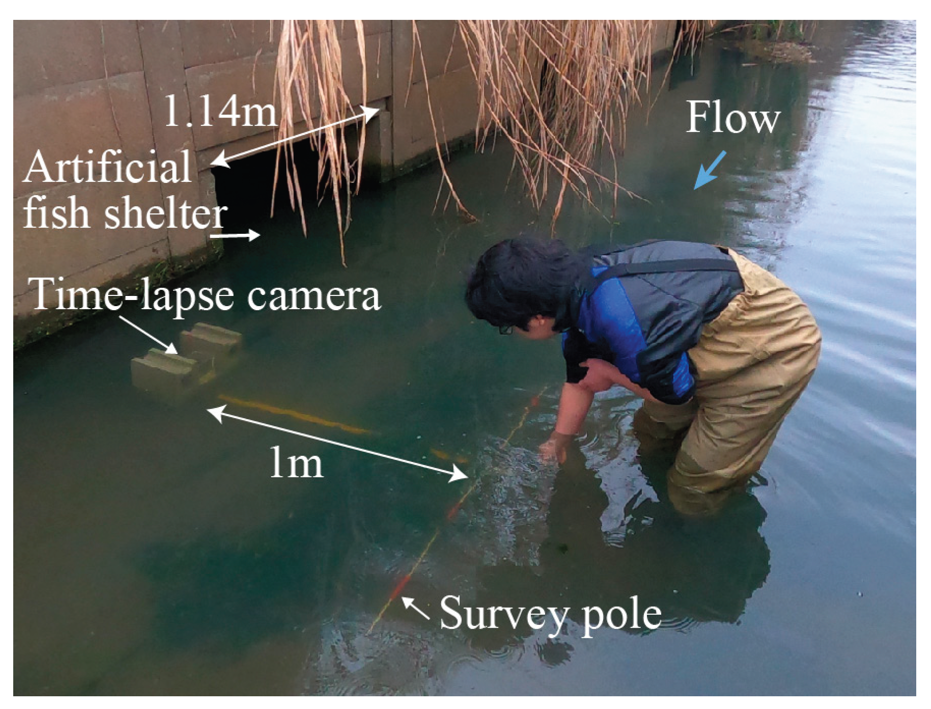
Figure 2.
F1-confidence curve.
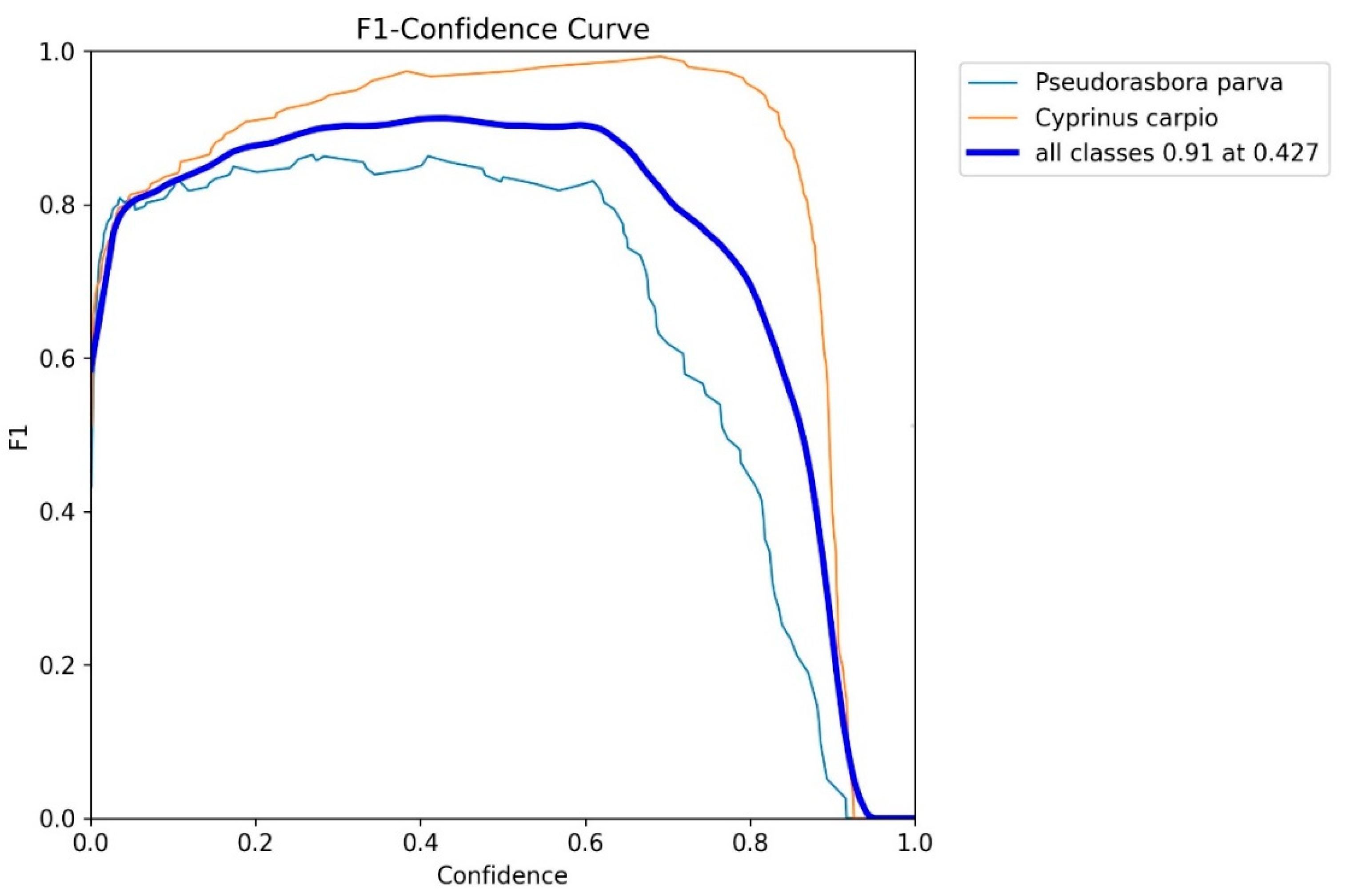
Figure 3.
A confusion matrix showing the detection performance of the YOLOv8n model on 300 randomly selected images from the inference dataset (12,600 images in total) was used to evaluate the validity of the fish detection results. The confidence and IoU thresholds used for the NMS were fixed at 0.427and 0.5, respectively.
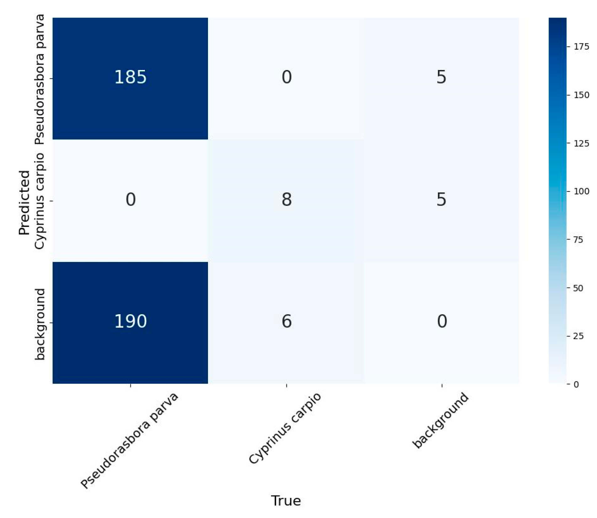
Figure 4.
Examples of successful detection during inference. All the objects were correctly identified with a confidence threshold of 0.427 and an IoU threshold of 0.50.
Figure 4.
Examples of successful detection during inference. All the objects were correctly identified with a confidence threshold of 0.427 and an IoU threshold of 0.50.
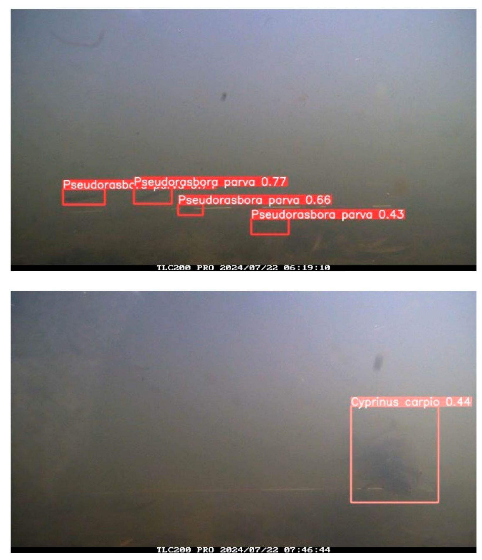
Figure 5.
Examples of images in which detection was difficult. (a) A floating object falsely detected as Pseudorasbora parva (FP); (b) P. parva not detected (FN), including fish that are difficult to classify by species; (c) a dark area falsely detected as Cyprinus carpio (FP); (d) C. carpio not detected (FN); and (e) two overlapping C. carpio individuals detected as a single fish (FN). Confidence threshold: 0.427; IoU threshold: 0.50.
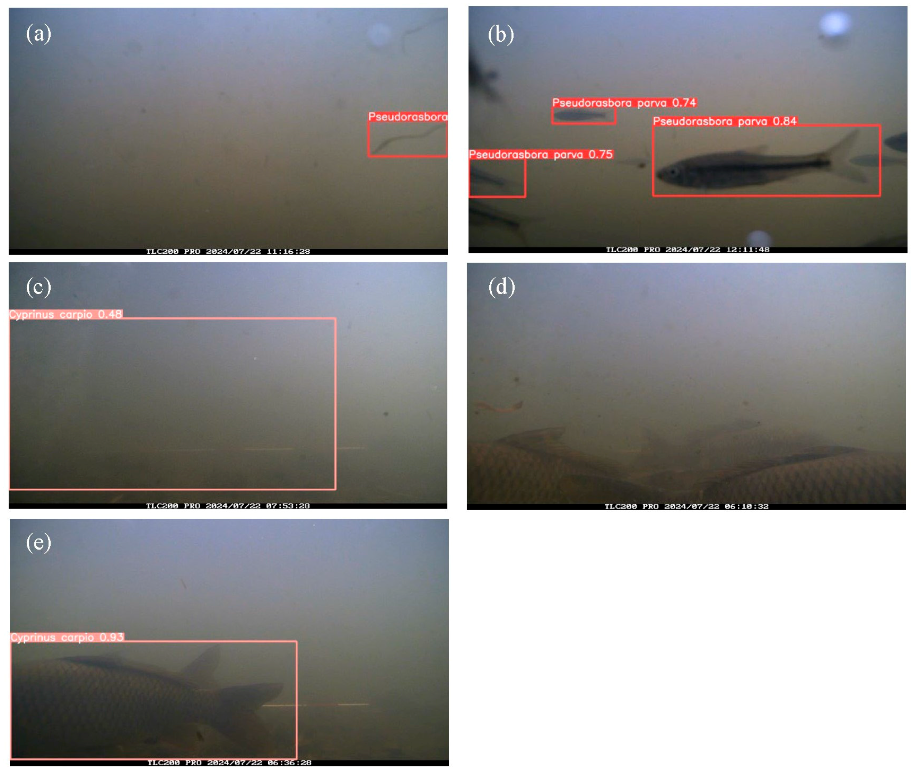
Figure 6.
Sensitivity analysis of the number of detected individuals with respect to the IoU threshold used for NMS during inference. The confidence threshold was set to 0.427.
Figure 6.
Sensitivity analysis of the number of detected individuals with respect to the IoU threshold used for NMS during inference. The confidence threshold was set to 0.427.
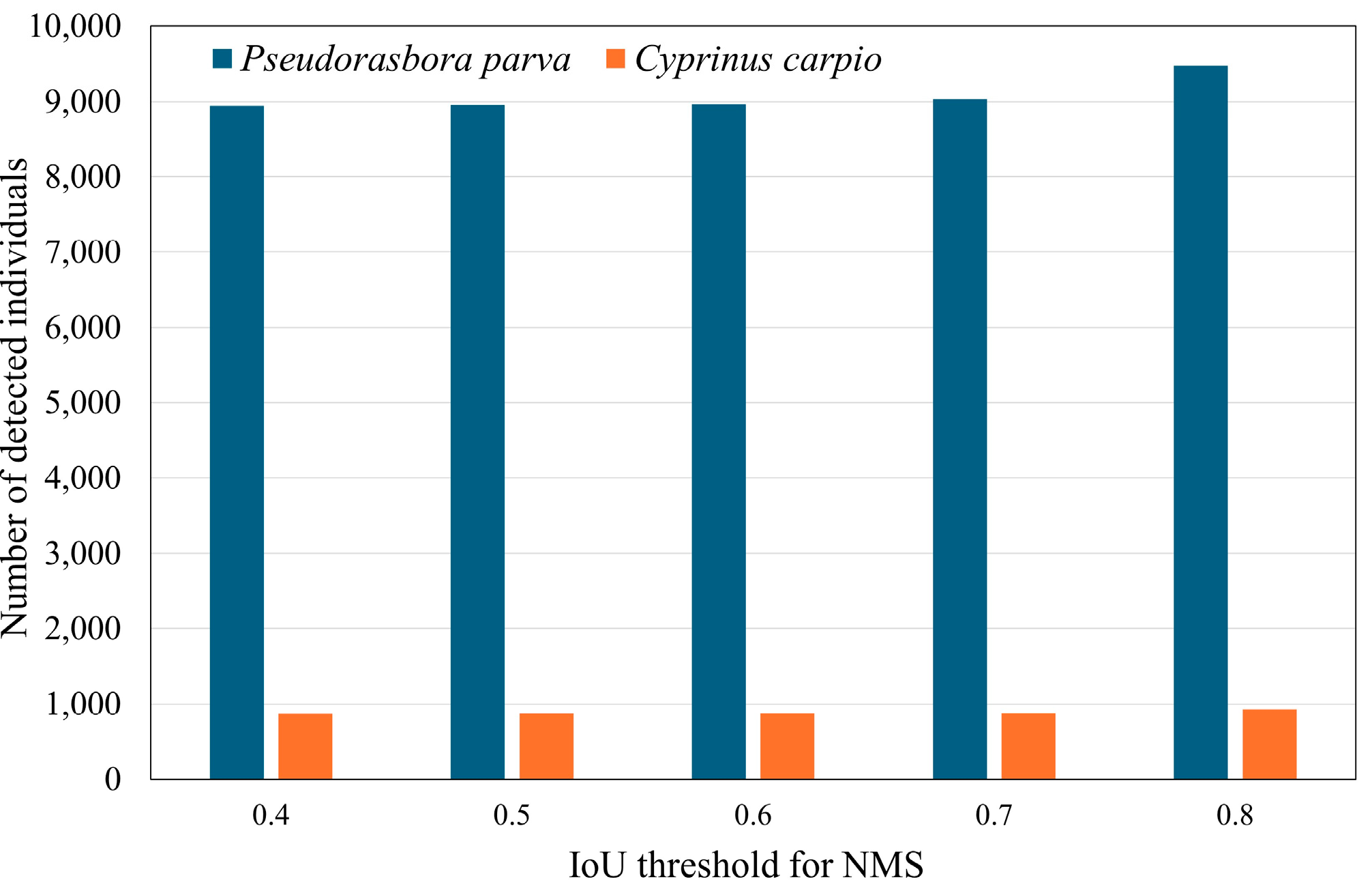
Figure 7.
Sensitivity analysis of the number of detected individuals with respect to the confidence threshold during inference. The IoU threshold used for the NMS was fixed at 0.5.
Figure 7.
Sensitivity analysis of the number of detected individuals with respect to the confidence threshold during inference. The IoU threshold used for the NMS was fixed at 0.5.
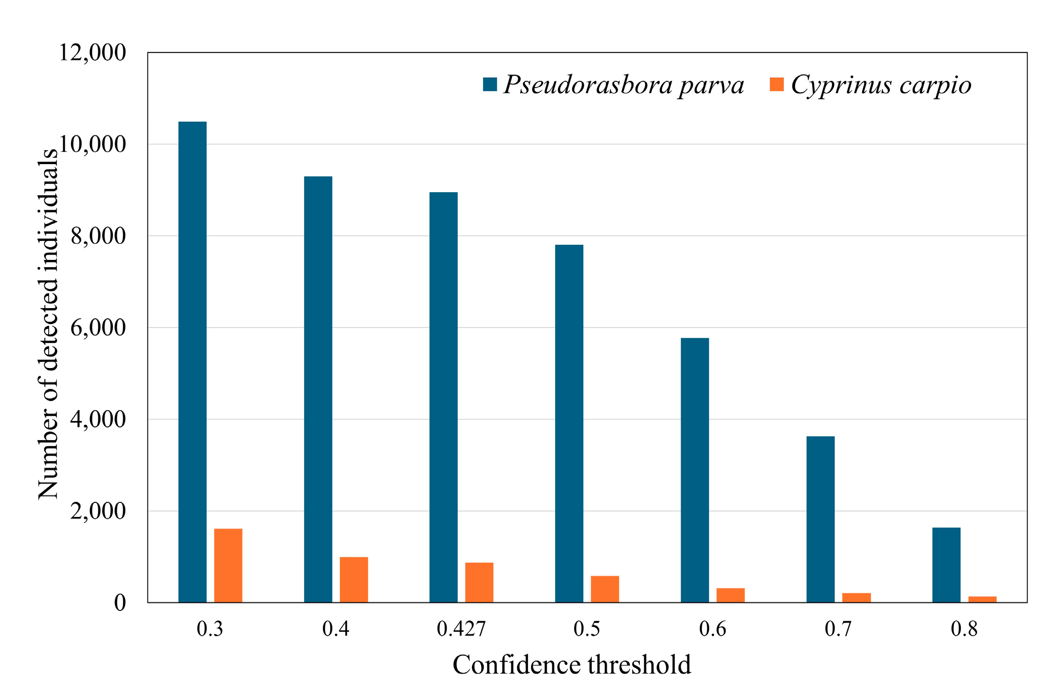
Figure 8.
Images and fish detection results from the appearance of the two Cyprinus carpio until they left the frames. Species and confidence scores are indicated by bounding boxes and labels with a confidence threshold of 0.427 and an IoU threshold of 0.5. Images were taken between 6:36:18 and 6:36:39 on July 22, 2024, at 2-second intervals.
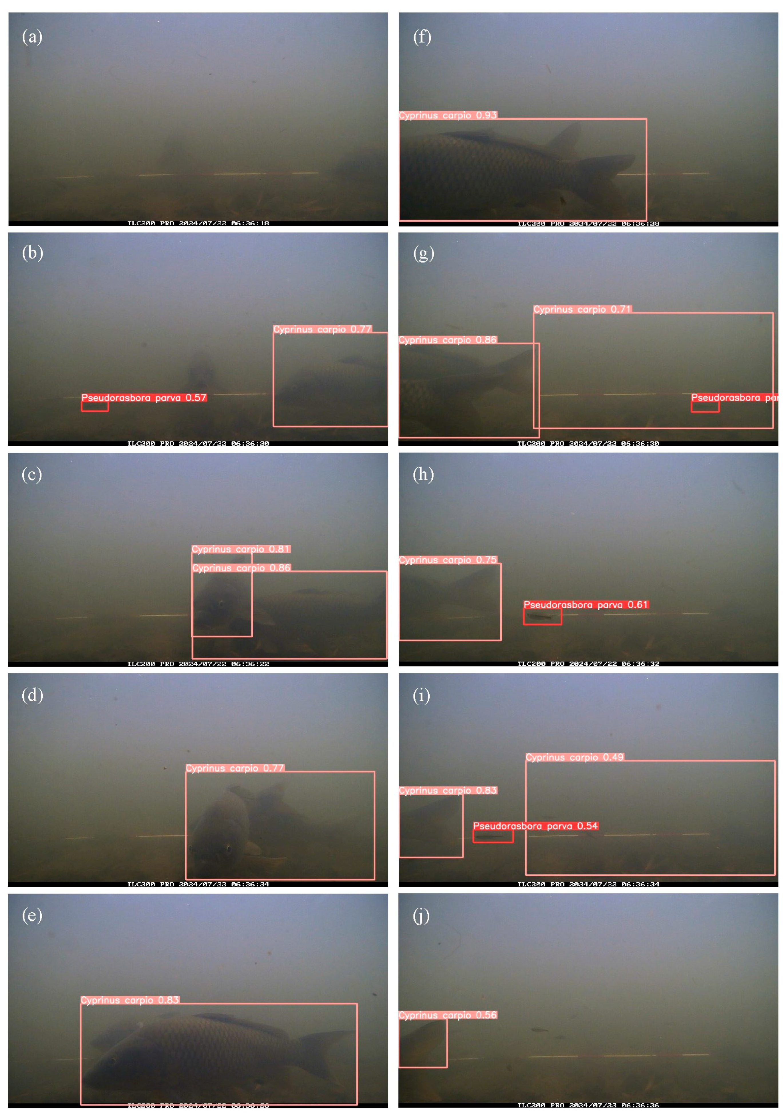
Figure 9.
Temporal variation in the 10-minute cumulative number of occurrences of (a) Pseudorasbora parva and (b) Cyprinus carpio estimated by the model. The IoU threshold was set to 0.5. Graphs with confidence thresholds of 0.427 for P. parva and 0.7 for C. carpio were presumed to best reflect the actual situation. According to the discussion in the main text, the black line in (a), corresponding to Conf = 0.427, and the black line in (b), corresponding to Conf = 0.7, were considered more reliable.
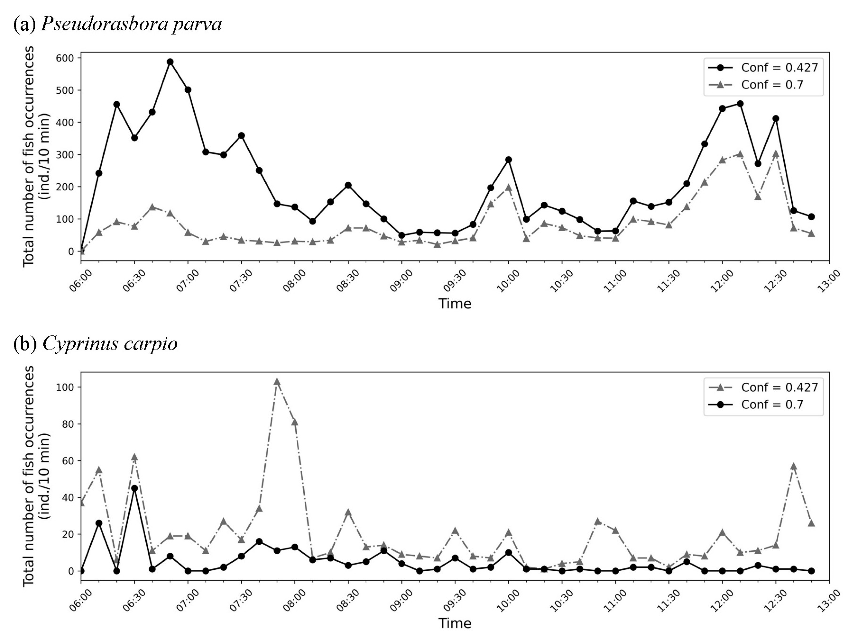

Table 1.
Summary of annotated training and validation datasets, including the number of images and fish instances per species.
Table 1.
Summary of annotated training and validation datasets, including the number of images and fish instances per species.
| Category | Training data | Validation data |
| Number of images (total) | 546 images | 129 images |
| Number of background-only images | 57 images | 14 images |
| Number of images with fish | 489 images | 115 images |
| Pseudorasbora parva | 305 individuals | 76 individuals |
| Cyprinus carpio | 333 individuals | 74 individuals |
Table 2.
Computational environment and hyperparameter settings for YOLOv8n training.
| Configuration | Parameter |
| GPU | NVIDIA Quadoro P4000 |
| Operating System | Windows 10 Pro, 64-bit |
| Python | 3.8.5 |
| PyTorch | 2.2.0+cu118 |
| CUDA | 11.8 |
| Optimizer | AdamW |
| Initial learning rate | 0.001 |
| β1 | 0.937 |
| β2 | 0.999 |
| Weight decay | 0.0005 |
| Learning rate scheduler | Linear decay |
| Epochs | 500 |
| Input Image Resolution | 960 × 960 pixels |
| Batch Size | 16 |
Table 3.
The performance metrics of the YOLOv8n model were evaluated on the validation dataset, including the Precision, Recall, F1 score, and mAP for each fish species.
Table 3.
The performance metrics of the YOLOv8n model were evaluated on the validation dataset, including the Precision, Recall, F1 score, and mAP for each fish species.
| Images | Instances | Precision(%) | Recall(%) | F1 score(%) | mAP50(%) | mAP50-95(%) | |
|---|---|---|---|---|---|---|---|
| All species | 129 | 150 | 95.1 | 88.4 | 91.6 | 95.5 | 69.0 |
| Pseudorasbora parva | 129 | 76 | 95.2 | 78.1 | 85.8 | 91.6 | 58.8 |
|
Cyprinus carpio |
129 | 74 | 95.0 | 98.6 | 96.8 | 99.4 | 79.1 |
Table 4.
The detection performance of the YOLOv8n model on 300 randomly selected images from the inference dataset illustrates its accuracy under practical conditions.
Table 4.
The detection performance of the YOLOv8n model on 300 randomly selected images from the inference dataset illustrates its accuracy under practical conditions.
| Images | Instances | Precision(%) | Recall(%) | F1 score(%) | mAP50(%) | mAP50-95(%) | |
|---|---|---|---|---|---|---|---|
| All species | 300 | 389 | 88.9 | 47.1 | 61.6 | 67.8 | 47.0 |
| Pseudorasbora parva | 300 | 375 | 96.5 | 37.0 | 53.5 | 72.0 | 48.7 |
|
Cyprinus carpio |
300 | 14 | 81.2 | 57.1 | 67.1 | 63.6 | 45.3 |
Disclaimer/Publisher’s Note: The statements, opinions and data contained in all publications are solely those of the individual author(s) and contributor(s) and not of MDPI and/or the editor(s). MDPI and/or the editor(s) disclaim responsibility for any injury to people or property resulting from any ideas, methods, instructions or products referred to in the content. |
© 2025 by the authors. Licensee MDPI, Basel, Switzerland. This article is an open access article distributed under the terms and conditions of the Creative Commons Attribution (CC BY) license (http://creativecommons.org/licenses/by/4.0/).
Copyright: This open access article is published under a Creative Commons CC BY 4.0 license, which permit the free download, distribution, and reuse, provided that the author and preprint are cited in any reuse.


