
Submitted:
15 July 2025
Posted:
18 July 2025
You are already at the latest version
Abstract
Accurate prediction of broiler shipment weight is essential for optimizing production planning and meeting market demand. Previous studies have estimated representative daily weight values from load cell data using K-means clustering and kernel density estimation (KDE), and have applied forecasting models such as Prophet, ARIMA, and Gompertz. Among these, the combination of K-means and Prophet demonstrated the best performance. In this study, we propose an enhanced method that integrates computer vision with load cell measurements. A YOLOv8-based object detection algorithm is employed to count the number of broilers on the load cell using real-time images captured by a camera. The average weight per broiler is estimated by dividing the total measured weight by the number of detected chickens. Based on the previously established forecasting framework, these more accurate values are fed into the Prophet model to predict shipment weight. Experimental results show that, compared with earlier methods, the proposed approach improves prediction accuracy by approximately 2.82%, enabling a better understanding of broiler growth patterns and providing more reliable support for shipment scheduling in smart poultry farms.
Keywords:
broiler weight prediction
; load cell
; object detection
; outlier handling
; smart poultry farming
1. Introduction
The livestock industry in South Korea faces numerous external challenges, including globalization, a declining agricultural population, and an aging society. These factors are making it increasingly difficult to maintain self-sufficiency in livestock and feed production. In contrast, smart livestock farming holds the potential to reduce resource waste and labor demands, thereby supporting sustainable and autonomous agricultural practices. In recent years, smart livestock management technologies based on big data and artificial intelligence have significantly improved productivity through advancements in breeding, nutrition, environmental control, and maintenance reduction [1].
In the poultry sector, South Korea has made continuous progress in meat quality and environmental management. However, the domestic self-sufficiency rate remains relatively low, with a heavy reliance on imports. In 2024, the total import volume of chicken breast, wings, and legs reached 184,716 tons, and this upward trend continued from January to April 2025 [2].
In Jeollabuk-do, determining the optimal shipment time for broilers has long been a major challenge for poultry farmers. According to standard broiler farming contracts, if the difference between the predicted and actual shipment weight is within ±50 grams, farmers receive a bonus of 3 KRW per kilogram. However, if the deviation exceeds this range, a penalty of 6 KRW per kilogram is imposed. Therefore, accurate weight prediction is directly tied to farmers’ income. Additionally, buyer requirements have become increasingly specific—for instance, distributors demand broilers weighing between 1.1–1.2 kg, school lunch suppliers require 1.7 kg, and processing companies request 1.9 kg. If the broilers fall outside the desired weight range, they must be sold as cut-up parts, which complicates operations and reduces profitability. As such, effective monitoring and prediction of broiler weight are essential for modern poultry farming. Some large-scale farms have already begun installing load cells and overhead cameras to collect growth data. However, numerous challenges arise during actual implementation. Most notably, load cells often struggle to distinguish between valid and anomalous data, or they apply overly strict standards, resulting in significant noise that negatively impacts the accuracy of predictive models [3].
In our previous research, we proposed a prediction framework capable of automatically collecting broiler weight data from smart farms in the Namwon and Wanju regions. To address the challenges posed by manual weighing and data noise, K-means clustering and KDE were applied to optimize the raw data and extract representative daily weight values. These values were then used as inputs for various time series forecasting models, including Prophet, Gompertz, and ARIMA. Among these, the K-means + Prophet combination achieved the best prediction performance, enabling stable forecasting without the need for manual measurement [4].
Building upon the aforementioned research framework, this study proposes an enhanced shipment weight prediction method that integrates computer vision with sensor measurements. The approach employs a YOLOv8-based object detection algorithm to accurately and efficiently identify and count the number of broilers on the load cell in real time. To improve detection accuracy, a center/edge region filtering strategy is applied to exclude images that may introduce noise or errors. Based on this, the total recorded weight from the load cell is divided by the number of detected chickens to estimate a more robust average weight per broiler. These representative weight values are then constructed into a time series and fed into the Prophet model for final shipment weight prediction. Experimental results demonstrate that the proposed method improves prediction accuracy by an average of 2.82% across five datasets, compared to conventional approaches. This algorithm offers a more reliable decision support tool for shipment scheduling in smart poultry farms and holds strong potential for practical application.
2. Background
2.1. Overview of Broiler Weight Prediction Methods
Predicting broiler weight is essential for optimizing production and determining shipment schedules. Traditional studies primarily employed nonlinear growth models such as the Gompertz model, Logistic model, and Von Bertalanffy model to fit broiler growth curves under various conditions [5,6,7,8,9,10,11,12]. These models generally offer high fitting accuracy, although their performance may vary depending on age and breed. Later research introduced dynamic neural networks that incorporate environmental data such as feed intake, humidity, and temperature, thereby improving prediction accuracy but also increasing data collection costs [13,14,15]. Although these methods have achieved success, most rely on ideal or manually optimized data, which limits their applicability in real-world scenarios.
monitoring and collecting broiler weight information can help farmers understand the growth status and trends of their flocks, allowing them to adjust feeding strategies accordingly. De Wet et al. [16] observed 50 broilers raised under commercial conditions to compare traditional manual weighing with automatic weighing systems. They used nonlinear regression to analyze the relationship between body weight and target surface pixel count, as well as between body weight and target contour pixel count. Mortensen et al. [17] used 3D computer vision technology combined with neural networks to predict broiler weight. The prediction error ranged from 10 to 100 grams in the early stage of broiler growth, and from 50 to 250 grams in the later stage. Amraei et al. [18] also employed 3D computer vision technology along with neural networks for broiler weight prediction. In the study [18], digital image processing techniques were used to extract features such as area, perimeter, convex area, major and minor axes, and eccentricity from broiler images, and a neural network was trained for weight prediction. This method achieved a prediction error of less than 50 grams. Liu et al. [19] used a depth camera and an electronic scale to perform individual weighing of broilers. After segmenting the broiler target regions, they applied KDE for adaptive gender classification. This method achieved a gender classification accuracy of 99.7% and an individual sampling rate of 77.32%. However, the study required 70 hours of manual effort to annotate the dataset. Although numerous research achievements have been made in the field of livestock weight prediction, these methods still face various practical challenges, such as differences in farming environments and high implementation costs [20].
2.2. Object Detection for Broiler Counting on the Weighing Platform
With the advancement of computer vision technology, image analysis methods based on object detection have been progressively applied to poultry quantity monitoring and individual weight estimation. In 2020, Guo et al. [21] employed an object detection approach to analyze broiler floor distribution, laying the foundation for real-time assessment tools to monitor broiler behavior and spatial patterns in commercial facilities. O. Geffen et al. [22] utilized the Faster R-CNN, a convolutional neural network (CNN)-based object detection algorithm, to automatically count caged laying hens. In 2022, Allan Lincoln Rodrigues Siriani et al. [23] achieved a 99.9% detection accuracy for chickens in low-quality videos using the YOLOv4 model. By 2024, Edmanuel Cruz et al. [24] adopted the YOLOv8 object detection model for precise chicken counting, while a comparative analysis with earlier models, including YOLOv5, highlighted YOLOv8's superior accuracy and robustness [25], demonstrating its strong practical potential. YOLO series of object detection algorithms, particularly YOLOv8, has emerged as one of the most performant and practical technologies for poultry quantity recognition, providing a reliable image-based foundation for broiler weight estimation.
2.3. Outlier Handling
After identifying the number of broilers, the load cell data can be used to estimate the average body weight per unit time. However, in actual production environments, automatically collected weight data are often affected by factors such as overlapping broilers, abnormal postures, feed residues, feces, or feather interference. These factors introduce significant outliers and noise into the sensor data. To ensure the accuracy and stability of the predictive model training, systematic outlier detection must be performed on the raw data prior to modeling.
2.3.1. IQR and Z-Score
Among common statistical methods, IQR (Interquartile Range) and Z-score (Standard Deviation Method) [26] are widely used for outlier detection in univariate data. The IQR method determines outliers by calculating the distance between the first quartile and third quartile, making it suitable for data with clear median trends. The Z-score method calculates sample deviations based on mean and standard deviation, making it applicable to normally distributed data. Both methods are computationally simple and efficient, but their effectiveness is limited when dealing with high-dimensional or asymmetrically distributed data.
2.3.2. DBSCAN
DBSCAN (Density-Based Spatial Clustering of Applications with Noise), originally proposed by Ester et al., can divide clustering regions based on density and automatically identify non-clustered "outliers", making it widely used in outlier detection tasks [27]. The algorithm determines whether a point belongs to a high-density region by defining two parameters: neighborhood radius (epsilon) and minimum number of points MinPts in the neighborhood. First, for any point in the dataset, its -neighborhood is defined as Equation 1. Here, represents the sample dataset, and denotes the distance between points and , typically calculated using Euclidean distance. If the -neighborhood of a point contains at least MinPts (the minimum point threshold), then is defined as a core point, i.e., . Furthermore, if a point lies within the -neighborhood of a core point , then is considered directly density-reachable from , provided is a core point.
During algorithm execution, all core points and their density-reachable points are clustered together. Points that are neither core points nor covered by any core point—that is, points that are not density-reachable—are labeled as "noise points" or outliers, as formally defined in Equation (2). Therefore, DBSCAN achieves automatic outlier detection while performing clustering tasks through its density-based rejection mechanism.
2.3.3. Isolation Forest
Isolation Forest is an unsupervised anomaly detection method based on the concept of "isolation". Its core principle is that anomalous samples, being sparsely distributed in the data space, can be isolated more quickly through random partitioning, while normal samples typically reside in dense regions and require more splits to be isolated [28].
The steps for anomaly detection with Isolation Forest are:
- Construct binary trees (Isolation Trees, iTrees) randomly from the training dataset;
- For a test sample , input it into all iTrees and record the path length required from the root node to complete isolation (reaching a leaf node) in each tree. Then calculate the average path length across all trees (Equation (3));
- The anomaly score is calculated according to Equation (4), where represents the theoretical expected path length for a sample size of , serving as a normalization factor for path lengths, as defined in Equation 5. where represents the approximation of the i-th harmonic number, with the constant being the Euler-Mascheroni constant;
- If , the sample x is highly likely to be an anomaly. If s, the sample x is generally considered normal. When all samples in the dataset yield scores close to 0.5, it indicates no significant anomalies exist in the dataset;
The Isolation Forest method leverages an intuitive combination of random tree structures and path lengths, offering significant advantages including high computational efficiency and strong scalability with data size.
2.3.4. One-Class Support Vector Machines
One-Class SVM (One-Class Support Vector Machines) is an unsupervised learning method commonly used for anomaly detection, proposed by Schölkopf et al. in 1999 [29]. Its core concept involves identifying an optimal hyperplane in a high-dimensional feature space that separates the majority of samples from the origin, thereby detecting anomalies that deviate from the primary data distribution. The model training process is achieved by solving a convex quadratic programming problem (Equations (6) and (7)).
Here, denotes the kernel function that maps input samples to a high-dimensional feature space. The slack variable permits some samples to reside inside the hyperplane, while the parameter controls the trade-off between model complexity and anomaly tolerance. The hyperplane offset determines the decision boundary position. After training, the One-Class SVM's discriminant function is given by Equation ()8.
where represents the Lagrange multipliers obtained by solving the dual optimization problem, subject to the constraints in Equation (9). A sample x is classified as anomalous when the decision function yields , and as normal when . Commonly used kernel functions include the Radial Basis Function (RBF) kernel (Equation 10). Here, denotes the bandwidth parameter of the kernel function, controlling the model's sensitivity to data variations. A smaller makes the model sensitive to local differences, while a larger emphasizes global trends. Furthermore, Schölkopf et al. demonstrated that the hyperparameter in One-Class SVM has clear statistical significance: it represents both the theoretical upper bound for the proportion of anomalies and the theoretical lower bound for the proportion of support vectors. Due to its effective handling of high-dimensional data, One-Class SVM has found widespread practical applications in sensor data analysis, image recognition, industrial data cleaning, and anomaly detection tasks, while maintaining strong generalization performance.
2.3.5. Mahalanobis
The Mahalanobis Distance [30] is a multivariate outlier detection method that accounts for correlations between data features, originally proposed by P. C. Mahalanobis in 1936. Unlike conventional Euclidean distance, the Mahalanobis distance effectively identifies outliers in multidimensional spaces with correlated features by incorporating the data's covariance matrix. For a given sample point x, its Mahalanobis distance from the dataset's centroid (mean vector) μ is defined by Equation (11).
Here, represents the feature vector of the sample being tested, denotes the mean vector of the dataset, is the covariance matrix of the dataset, and represents the inverse of the covariance matrix. In anomaly detection tasks, the Mahalanobis distance is typically employed to measure how significantly a sample deviates from the center of the overall data distribution. When a sample's Mahalanobis distance substantially exceeds the average level of other samples, it can be identified as a potential outlier. For livestock sensor data - such as broiler weight, body size characteristics, or other high-dimensional features where strong correlations may exist - the Mahalanobis distance serves as a robust and effective anomaly detection method. It helps identify outliers or noisy data that may occur during data collection, thereby enhancing the prediction accuracy and reliability of models.
3. Materials and Methods
3.1. Data Collection
This study utilizes a dataset collected from broiler farms operated by a poultry company in Jeollabuk-do, South Korea. The farm specifications are illustrated in Figure 1. Each farm measures 70-80m in length and 19m in width, with sidewall heights of 4m and roof heights of 6.5m. The facilities have a maximum capacity of approximately 30,000 Cobb500 broilers per rearing cycle. The raw dataset comprises at least three data categories: weight measurements, temporal data, and image data. For comprehensive monitoring, we deployed IoT-enabled weighing sensor devices (Emotion Co., Ltd.'s Kokofarm broiler live weight meter) across three strategic locations in the broiler resting areas - front, middle, and rear sections - to capture both weight metrics and broiler count data.
Additionally, we installed overhead cameras above each weighing sensor to acquire visual data. Figure 2 displays the camera positioning and captured footage. When the automated weighing device detects value fluctuations, it indicates broilers have either stepped onto or departed from the weighing platform. For locally recorded data, we implemented a filtering protocol that eliminates measurements below 10g or exceeding 2500g. The validated data is transmitted hourly to cloud databases via Integrated Gateway (IoT G/W) devices for subsequent analysis.
The algorithm was applied to five datasets collected from broiler farm KF0081 between November 2023 and January 2025, with detailed dataset specifications provided in Table 1. Each dataset contains per-second weight measurements and image data recorded continuously from the initial rearing stage through to the shipping date. Across the approximately 29-35 day rearing cycles, the datasets encompassed between 2,030,085 and 2,745,771 images. Variations in dataset sizes primarily stemmed from differences in broiler growth rates that affected rearing durations, along with data gaps caused by equipment malfunctions and recording adjustments due to canceled or modified shipment schedules. The saved images follow a naming convention consisting of: farm name + houseID + scaleID + year-month-day + hour-minute-second + weight(g) (representing the load cell value in grams). The images are stored in JPEG format as 320×240 pixel RGB images.
Based on the originally collected image data, we further processed and annotated the images to construct a high-quality dataset suitable for object detection model training. As shown in Figure 3, during the 0-35 day rearing period, we randomly sampled images from the complete set at 4-day intervals, totaling 463 images. These images were manually annotated using the LabelImg tool, with the annotation category limited to “broiler” to ensure target consistency and dataset focus. Among these, 367 images were used for training, while 96 images (48 each for validation and testing) were allocated for model performance evaluation. To improve detection accuracy, the image samples covered broilers at different ages, postures, quantities, and occlusion conditions, aiming to reproduce the image diversity encountered in real farming environments as comprehensively as possible. Figure 3(a) displays the total number of annotated targets at each age, while Table 2 provides the corresponding number of images for each age group.
Beyond the metrics generated during the object detection model training, this study performed manual verification on the processed images from the 2023_1117_KF0081_01-Img_Data dataset to further evaluate the model's practical performance. The verification methodology involved: randomly selecting 180 detected images per day (totaling 5,040 images) across different age groups, with each image manually inspected to validate the accuracy of the model's broiler counting on load cell platforms. The evaluation results were classified into three categories: (1) detected count matching actual number (True Positive), (2) discrepancy between detection and actual count (False Positive), and (3) severely blurred/occluded images where accurate counting was unverifiable (Human Uncertain). This assessment complements quantitative metrics by demonstrating the model's robustness under varying rearing ages, stocking densities, and lighting conditions in real-world applications.
To validate the effectiveness of the edge/center region strategy in improving weight data quality, this study selected 14,115 images generated between 2024-05-21 03:59:58 and 2024-05-21 07:59:59 from the 2024_0502_KF0081_02-Img_Data dataset as experimental samples. In this experiment, three different edge/center region boundary configurations were applied to detect broilers in the images, and the average weights of broilers located in edge regions versus center regions were calculated. By comparing the weight distribution differences between these two regions, we verified whether edge regions would introduce significant bias to the final average weight estimation, thereby evaluating the efficacy and rationale of this regional filtering strategy for data cleaning and representative sample extraction.
3.2. Algorithm Composition and Design
The broiler shipment weight prediction algorithm proposed in this study consists of three main steps: detecting the number of broilers on the load cell, determining representative average weight values, and predicting shipment weight. The collected data were grouped by age (in days) for processing the weight measurements and image data recorded per second.
An object detection approach was employed to identify broilers in the images and assign corresponding headcount labels to each weight measurement. To enhance data reliability, a center/edge region discrimination strategy was implemented: weight data associated with images where broilers were detected in the edge regions of the load cell were discarded as potentially interfered, while only data from images showing broilers exclusively in the central region were retained.
After obtaining the weight distribution, more robust average weight values were derived by dividing each weight measurement by its corresponding broiler count. Six distinct methods were then applied to calculate the daily average weights:
- Raw Mean: Direct calculation without any preprocessing;
- IQR + Z-score;
- DBSCAN;
- Isolation Forest;
- One-Class SVM;
- Mahalanobis.
The mean was computed following outlier removal. These procedures generated time-series data of daily average weights, which were subsequently fed into the Prophet model for shipment weight prediction. The predictive performance of each method was comparatively analyzed. The complete algorithmic workflow is illustrated in Figure 4.
For the broiler counting stage, this study constructed an object detection model using image datasets collected from the start of rearing to shipment to estimate the number of broilers appearing on the load cell in each frame. Regarding model selection, priority was given to the YOLOv8n model from the YOLOv8 detection framework, which combines lightweight characteristics with high accuracy. This model represents the most parameter-efficient and computationally optimal lightweight version in the YOLOv8 series, making it suitable for edge device deployment and real-time detection requirements. The input image size was set to 320×320 pixels. The model was trained for 300 epochs with a batch size of 32 images per iteration. The random seed was fixed at 1, while other parameters followed Ultralytics YOLOv8's default settings. Training was conducted in a PyTorch environment. Detailed specifications of the experimental equipment are presented in Table 3.
The object detection model trained through the aforementioned steps enables real-time analysis of images captured every second. In actual farm environments, load cells are installed on the floor area inside the poultry house to record instantaneous body weights of individual broilers. However, when broilers stand non-vertically on the weighing platform or only partially lean against the edge regions, it results in abnormal weight measurements, thereby introducing bias into the overall weight distribution. Such errors are difficult to eliminate through conventional methods in large-scale automated monitoring systems, necessitating the implementation of a spatial region judgment mechanism based on image analysis to filter unreliable data.
To address this issue, this study proposes a discrimination method using Central Region and Peripheral Region. This approach distinguishes between reliable and unreliable weight measurements by determining the position of the detection bounding box center points from the object detection model. Samples with detection box center points located within the Central Region are considered valid, while those with center points falling in the Peripheral Region are classified as uncertain, and their corresponding weight data are subsequently discarded.
To validate the effectiveness of this regional division strategy, this study designed three edge/center region configuration methods (Figure 5) and conducted comparative experiments using the same dataset, as detailed below:
- Experiment A (Basic Configuration):
A 10-pixel wide edge region was created by extending 5 pixels inward and outward from the weighing platform boundary, with the interior area designated as the central region;
- Experiment B (Center Contraction):
Building upon Experiment A, the central region was further reduced by 5 pixels inward, thereby expanding the edge region to 15 pixels in width. This configuration enables more stringent elimination of edge interference in the central region;
- Experiment C (Edge Expansion):
Based on Experiment A, the edge region was extended outward by an additional 5 pixels, similarly achieving a 15-pixel width for the edge region. This setup evaluates the stability impact under more rigorous edge region settings.
During the process of collecting broiler weight data using load cells, sensor data anomalies frequently occur due to the complexity of actual farming environments. Therefore, in the broiler shipment weight prediction framework proposed in this study, outlier cleaning has been implemented as a critical preprocessing step. Its objective is to eliminate abnormal weight measurements caused by non-growth factors such as equipment errors and behavioral interference, thereby enhancing the stability and representativeness of average weight estimations. This process provides more authentic and continuous broiler weight change curves for time series modeling. The study incorporates five classical anomaly detection methods suitable for unsupervised scenarios.
This study first employs the IQR (Interquartile Range) method for preliminary data cleaning. The specific approach involves using a 15-minute time window to locally model the distribution of weight measurements within each window. For each window, we calculate the first quartile () and third quartile () of the data, then compute the interquartile range . All data points below or above are identified as outliers and removed from the sample set. Building upon the IQR cleaning, we further apply the Z-score method within the same 15-minute sliding windows to eliminate any remaining extreme values. This additional step calculates the mean () and standard deviation () of the remaining data, with any values satisfying being flagged as anomalies.
In DBSCAN-based outlier detection, to avoid bias from manual parameter setting, this study adopts the elbow point detection method proposed by Satopaa et al. [31]. The method identifies the optimal eps value by analyzing the k-nearest neighbor distance plot, which has been effectively applied in multiple outlier detection and clustering studies [32]. The specific procedure is as follows: First, compute the distance between each sample point and its k-th nearest neighbor (set to 5 in this study) to construct a k-distance graph. Then, use the elbow method (KneeLocator) to determine the optimal inflection point as the final eps value. After performing DBSCAN clustering with this eps and , noise points are excluded, while samples from the main clusters are retained. The mean weight of these samples is calculated as the representative broiler weight value.
For outlier detection using the Isolation Forest algorithm, this study configured the number of estimators (n_estimators) as 100 and set the contamination rate to 0.03, indicating that approximately 3% of the total samples were expected to be outliers. A fixed random seed (random_state = 42) was established. After model training, each record was assigned an anomaly score and corresponding label, with samples labeled -1 identified as outliers and subsequently removed from further processing. Only normal samples labeled 1 were retained, and their average weight values within each time window (age in days) were calculated to serve as representative broiler weight measurements for the respective periods.
In the One-Class SVM method, we first standardized the original weight data using StandardScaler to achieve zero-mean and unit-variance distribution, thereby eliminating the influence of feature scales on the model. We then employed the Radial Basis Function (RBF) as the kernel function, with parameter nu set to 0.03 to limit the proportion of anomalous samples to no more than 3%. The gamma parameter was configured as 'auto', allowing automatic estimation of the kernel width based on the number of features. After model training, samples identified as anomalies (labeled -1) were removed from the dataset, retaining only normal samples for subsequent statistical analysis of average broiler weights.
In the Mahalanobis distance method, for each sample point, we calculate its Mahalanobis distance from the overall mean. Using the chi-square distribution critical value (with 2 degrees of freedom) at a 0.975 confidence level as the threshold, we determine whether the sample is an outlier. Samples exceeding this threshold distance are identified as anomalies and removed, retaining only normal samples for subsequent average weight calculations and time series construction.
The shipment weight prediction method follows the research framework established in reference [4]. The daily average weights, processed through different outlier detection methods, are constructed into time series data and used as input for the Prophet model. When the average weight first exceeds 1000 grams at a certain age, it is considered to enter the predictable phase. Therefore, this study uses the time series after the weight reaches 1000 grams as the prediction interval, employing the Prophet model to forecast broiler shipment weights. The prediction results from various outlier treatment methods are obtained and comparatively analyzed.
Figure 6 presents a comparative analysis of shipment weight predictions obtained from six different methods. The blue scatter points represent raw weight data, with point transparency (alpha) set to 0.004 to reduce visual clutter in high-density regions. Red circular markers indicate representative weight values selected within the age range where daily weights had not yet exceeded 1,000g. Black circular markers denote representative values from days when weights surpassed 1,000g, which were excluded from Prophet model training. Blue star markers show the model-predicted shipment weights, while green stars represent actual average shipment weights. This comparative visualization enables evaluation of how different outlier cleaning methods affect prediction accuracy.
3.3. Performance Evaluation of the Algorithm
This study aims to achieve effective prediction of broiler shipment weights through the proposed algorithm. To validate the prediction performance, we conducted a comprehensive comparison of the predictive models generated by six representative processing methods, with particular focus on evaluating how different outlier detection strategies impact final prediction accuracy. Using five broiler farming datasets as test subjects, we compared the Prophet model's output predictions against actual average shipment weight labels to calculate prediction error percentages. For evaluation metrics, we employed three standard measurements: Mean Absolute Error (MAE), Mean Absolute Percentage Error (MAPE), and Root Mean Squared Error (RMSE), providing a complete assessment of each method's prediction precision and robustness.
4. Results
4.1. Experiments in Object Detection Evaluation
To comprehensively evaluate the performance of the trained YOLOv8n model on the broiler image dataset, this study adopted standard evaluation metrics and presents Precision-Recall (P-R) curves and F1-Confidence curves (Figure 7). The P-R curve visually demonstrates the model's precision variations at different recall rates, reflecting its stability across various detection difficulty scenarios. Results show that the YOLOv8n model achieved a mean Average Precision (mAP@0.5) of 0.987 at an IoU threshold of 0.5, indicating exceptionally high detection accuracy. The F1 score-Confidence curve illustrates the model's balanced performance between precision and recall across different confidence thresholds. Experimental results demonstrate that when the confidence threshold is set to 0.593, the model achieves an F1 score of 0.96, representing the optimal region of the curve. This indicates that at this threshold, the detection boxes maintain both low false positive rates and high recall rates, making it suitable as the lower confidence bound for practical deployment.
To further validate the practical application effectiveness of the object detection model, this study conducted manual verification on the detection results from the previously sampled images, with statistical analysis performed on recognition accuracy across different age stages. The image recognition results were categorized into three classes: True Positive, False Positive, and Human Uncertain. The image verification results are shown in Figure 8, with True Positive represented by blue points, False Positive by orange points, and Human Uncertain by green points. The scatter plot was generated according to the following criteria: only images without broilers detected in the peripheral region and with at least one broiler identified in the central region were retained. For these qualified images, the total weight recorded by the load cell was divided by the number of broilers detected in the central region to calculate the average body weight per broiler, which was then used to create the age-versus-weight scatter plot. The verification results of the 5,040 sample images (180 randomly selected per day) were analyzed across three age groups. During the 0–10 day period, the average recognition accuracy was 94.6% (True Positive), with a 4.0% False Positive rate and 1.4% Human Uncertain cases. The 10–20 day period showed improved performance with 97.6% True Positive accuracy, a 1.7% False Positive rate, and 0.7% Human Uncertain. The model demonstrated optimal stability in the 20–28 day period, achieving 99.7% True Positive accuracy while maintaining merely 0.1% False Positive rate and 0.2% Human Uncertain rate. These results clearly indicate that the model's counting performance improves significantly as broilers grow larger, particularly showing exceptional accuracy after 20 days of age with near-perfect recognition capability during the final rearing phase.
Furthermore, analysis of the weight distribution patterns among sampled categories reveals distinct differences in scatter plot trends. Correct Detection samples (blue points) predominantly cluster along a stable growth curve, demonstrating a consistent upward trajectory with increasing age that accurately reflects normal broiler weight progression. This distribution pattern confirms the object detection model's strong stability and capacity to characterize weight development trends. In contrast, Incorrect Detection samples (orange points) exhibit more dispersed distributions across all growth stages, frequently deviating from the primary growth curve. Notable anomalies include unrealistically high weight readings during early stages and abnormally low measurements in mid-to-late phases, indicating persistent misjudgment risks when processing edge cases or severely occluded images.
4.2. Evaluation Experiments of Edge/Center Region Strategy
To further enhance the accuracy of individual broiler weight estimation in images, this study introduced an edge/center region identification strategy and conducted systematic evaluation on actual datasets. Figure 9 presents weight distribution characteristics under different region configurations and detection scenarios, where A, B, and C represent distinct edge/center region division strategies: A denotes the baseline configuration (10-pixel edge region width), B indicates inward contraction of the central region based on A (expanding edge region to 15-pixel width), and C represents outward extension of the edge region from A (also achieving 15-pixel edge width). The numerals 1, 2, and 3 indicate the detected broiler counts on the load cell platform, calculated as the sum of broilers detected in both central and edge regions. For instance, B2 represents detection of 2 broilers on the weighing platform under configuration "B", which may be distributed across both edge and central regions.
Figure 9 displays the temporal distribution of detected individual broiler weights (unit: g), where differently colored points represent distinct regional classification conditions. Green points indicate images where broilers were detected exclusively in the central region with no presence in edge areas – these samples are considered relatively reliable representative data. Red points correspond to images where at least one broiler was detected in edge regions, while the total count (sum of broilers in both central and edge regions) matches the labeled classification (“1 broiler”, “2 broilers” or “3 broilers”). All points represent estimated “individual broiler weights” (total weight divided by broiler count), demonstrating weight fluctuations under different configurations and detection conditions. The following observations are evident across different configurations:
Green points exhibit more concentrated distributions and stable weight ranges, demonstrating superior representativeness and predictability.
Red points show greater dispersion and higher variability, indicating edge region detection is more vulnerable to occlusions, posture variations, or weighing platform edge effects, resulting in data deviations.
Increasing broiler counts (from 1 to 3) correlate with elevated distribution dispersion, where red points progressively diverge from green clusters, suggesting that concurrent multi-broiler presence with edge region occurrences may magnify individual weight estimation errors.
These verification results collectively support prioritizing central region identification for representative value selection, while confirming edge regions’ potential to introduce measurement noise that compromises subsequent weight prediction accuracy.
4.3. Experiments in the Shipping Weight Prediction Step
Based on Configuration A of the edge/center region discrimination strategy, we detected broiler counts on the weighing platform and categorized corresponding weight values. As illustrated in Figure 10, key observations emerge: during early rearing (days 4-14), images with single broilers on the platform were scarce. Conversely, images showing 2-4 broilers simultaneously occurred more frequently, resulting in most early weight recordings being derived from multi-broiler combinations. This pattern indicates that smaller broiler size and denser activity in early stages promote concurrent platform occupancy, limiting acquisition of adequate single-broiler images for representative weight estimation. As broilers aged, single-occupancy rates increased, with weight distributions progressively converging toward physiologically plausible ranges.
After obtaining the individual broiler weight distribution, this study employed six methods to extract daily representative weight values. Using day 7 as an example (shown in Figure 11), the Raw Mean approach (without any outlier removal) contained numerous upper-bound outliers, yielding an average weight of 170g, with fewer but still present lower-bound anomalies. The IQR + Z-score method demonstrated the most aggressive outlier elimination, substantially removing extreme values while showing signs of over-cleaning (average weight: 168g). Isolation Forest and Mahalanobis distance methods exhibited more balanced boundary-sample retention, being slightly more conservative than IQR+Z-score (average weights: 168g and 167g respectively). One-Class SVM performed comparably but retained more marginal samples (average weight: 169g).
DBSCAN displayed optimal cleaning results visually. Its density-based clustering effectively identified and flagged isolated values while preserving the primary distribution area, ultimately producing an average weight (170g) identical to the raw data. These comparative results reveal significant differences in outlier detection sensitivity among methods, with DBSCAN demonstrating particularly strong robustness and representative value estimation capability for this dataset.
Figure 12 presents the daily representative broiler weights extracted by six different methods. It can be observed that although these methods vary in outlier detection intensity, the resulting representative weight data demonstrate consistent overall trends, with only minor differences of a few grams in average weights across age groups. These results not only validate the stability of each method in extracting representative values but also indirectly confirm the effectiveness of the preliminary object detection method for identifying broiler counts on the weighing platform.
Figure 13 demonstrates the application effects of two previously studied broiler weight representation extraction methods – K-means clustering and KDE - across different age stages. The results reveal that during days 4-14, the scarcity of single-broiler occurrences on the weighing platform makes it difficult to effectively extract density-based aggregation regions from individual weight distributions. Consequently, both methods frequently fail to identify clear representative values during this period. For instance, the K-means approach could not form valid clusters from days 11-14, forcing researchers to estimate missing age values through growth curve interpolation. This limitation highlights the instability of relying solely on weight-value density for representative extraction during early rearing phases. In contrast, our proposed strategy integrates object detection results with edge/center region identification, enabling relatively stable value estimation even when early-stage single-broiler weight data is scarce.
Table 4 presents the experimental results. Evaluated using three metrics—MAE, MAPE, and RMSE—the K-means and KDE methods exhibit significantly higher errors (MAE: 94.94 g and 117.36 g, respectively), highlighting their sensitivity to early-stage data scarcity and the presence of outliers. In contrast, the Raw Mean and IQR + Z-score ap-proaches show substantially reduced errors, suggesting improved robustness. The four advanced methods—DBSCAN, Isolation Forest, One-Class SVM, and Mahalanobis Dis-tance—demonstrate stable performance across all evaluation metrics, with the Ma-halanobis Distance method achieving the best overall results: MAE of 41.82 g, MAPE of 2.43%, and RMSE of 47.88 g. The proposed Mahalanobis method demonstrates a 2.82% higher MAPE than K-means, while DBSCAN, Isolation Forest, and Mahalanobis all maintain MAE and RMSE below 50g.
5. Discussion
The proposed method causes no disruption to farmers' existing rearing environments, as its implementation requires no modifications to current farming workflows regarding image capture or load cell equipment configuration, demonstrating excellent deployability. The integration of image recognition with weight sensor data significantly enhances the reliability of representative weight values, maintaining stable judgment criteria even when individual broiler weight data is sparse or contains interference factors. Unlike traditional methods limited to shipment weight prediction, our approach generates real-time representative average weight values for broiler populations throughout the entire rearing cycle, providing farm managers with continuous weight monitoring capabilities to support more precise feeding control and anomaly detection.
Although the Mahalanobis method achieved optimal prediction accuracy, the DBSCAN approach demonstrates superior robustness and interpretability in outlier identification and boundary value processing from the perspective of growth monitoring throughout the rearing process. Therefore, when considering both practical application scenarios and precision performance, the DBSCAN method holds greater value for practical implementation and wider adoption in this study.
Meanwhile, this study still presents aspects worthy of further exploration and optimization. First, the timing of prediction initiation warrants discussion. The current study defaults to initiating predictions when average weight reaches 1000g, based on industry standards where target shipment weight typically equals 1500g. However, some actual shipment weights in our dataset exceeded 1700g, substantially extending the prediction window and consequently increasing error accumulation. Given that weight fluctuations near shipment contribute more significantly to final weights, future studies could dynamically adjust prediction starting points according to contract-specific target weights to enhance model applicability and accuracy. Second, the edge region configuration in object detection requires refinement. While edge regions currently serve to exclude unreliable detection data when counting individual broilers, their fixed-width setting disregards actual broiler size progression. Specifically, early-stage broilers' smaller sizes may lead to over-exclusion with fixed edges, whereas later stages may require broader edges to effectively filter edge misdetections. Two potential dynamic edge strategies merit investigation: 1) Implementing nonlinearly increasing functions (e.g., parameterized sigmoid) to automatically adjust edge width according to growth patterns; or 2) Setting edge proportions based on detected bounding box areas for adaptive adjustment. Validating and implementing these optimizations will require extensive empirical work, offering fruitful directions for future research.
6. Conclusions
This study proposes a method for estimating daily representative broiler weights by integrating image-based object detection with load cell data. The approach effectively addresses the instability of density-based methods such as K-means and KDE during the early rearing stages, where single-broiler weight data is often sparse. By incorporating object detection to identify the number of broilers on the weighing platform and applying multiple outlier detection algorithms (IQR + Z-score, DBSCAN, Isolation Forest, One-Class SVM, and Mahalanobis distance), the proposed method significantly improves the stability and accuracy of representative weight extraction throughout the production cycle. Experimental results indicate that all six methods produced consistent overall weight trends, with only minor differences in representative values. Among them, the Mahalanobis method achieved the best performance in terms of MAE, MAPE, and RMSE. However, during the mid-rearing period, the DBSCAN method provided more accurate and robust representation of the group’s average weight, making it more suitable for real-time monitoring applications. The methods based on DBSCAN, Isolation Forest, and Mahalanobis distance all achieved MAE and RMSE values below 50g, which fall within the acceptable error range for average shipment weight specified in standard broiler farming contracts.
For future improvement, we identify two promising directions: (1) dynamically setting prediction onset based on target shipping weights to avoid extended-window errors, and (2) adapting edge exclusion strategies in detection according to broiler growth patterns. These enhancements will further strengthen the model's applicability in diverse real-world farming conditions.
Author Contributions
The author L.Y. collected and organized the data, conducted the idea of solving the problem addressed in this paper, and analyzed the data. He also designed the methodology and wrote the first draft of this paper. The author J.S. conceptualized this study and designed the methodology. He also managed the project and reviewed and revised the first draft of this paper. All authors have read and agreed to the published version of the manuscript.
Funding
This research was supported by Korea Institute of Planning and Evaluation for Technology in Food, Agriculture and Forestry(IPET) and Korea Smart Farm R&D Foundation(KosFarm) through Smart Farm Innovation Technology Development Program, funded by Ministry of Agriculture, Food and Rural Affairs(MAFRA) and Ministry of Science and ICT(MSIT), Rural Development Administration(RDA), grant number RS-2025-02216818.
Institutional Review Board Statement
Not applicable.
Data Availability Statement
The data set generated and analyzed in this paper cannot be publicly released due to the proprietary rights of Emotion Co., Ltd., Republic of Korea. However, it is available from the corresponding author upon research request with reasonable justification.
Acknowledgments
During the preparation of this manuscript, the authors used ChatGPT (free version) and DeepSeek (free version) for the purposes of translation, and used Google Translate for confirmation. The authors have reviewed and edited the output and take full responsibility for the content of this publication.
Conflicts of Interest
The authors declare no conflicts of interest.
References
- Choi, H.-C.; Kim, D.-H.; Kim, E.-T.; Lee, H.-J.; Park, J.-H.; Kim, J.-B.; Lee, J.-Y.; Jeon, J.-H.; Ki, K.-S.; Kwon, K.-S. Livestock Production in Korea: Recent Trend and Future Prospects of ICT Technology Livestock Production in Korea: Recent Trend and Future Prospects of ICT Technology.
- Korea Meat Distribution and Export Association Available online: http://www.kmta.or.kr/kr/data/stats_import_chicken_month.php (accessed on 7 July 2025).
- Oh, Y.; Lyu, P.; Ko, S.; Min, J.; Song, J. Enhancing Broiler Weight Estimation through Gaussian Kernel Density Estimation Modeling. Agriculture 2024, 14, 809. [CrossRef]
- Lee, B.; Song, J. Development of an Algorithm for Predicting Broiler Shipment Weight in a Smart Farm Environment. Agriculture; Basel 2025, 15. [CrossRef]
- Beiki, H.; Pakdel, A.; Moradi-Shahrbabak, M.; Mehrban, H. Evaluation of Growth Functions on Japanese Quail Lines. The Journal of Poultry Science 2013, 50, 20–27. [CrossRef]
- Al-Samarai, F.R. Growth Curve of Commercial Broiler as Predicted by Different Nonlinear Functions. American Journal of Applied Scientific Research 2015, 1, 6–9.
- Araújo, C.C.; Rodrigues, K.F.; Vaz, R.G.M.V.; Conti, A.C.M.; Amorim, A.F.; Campos, C.F.A. Analysis of Growth Curves in Different Lineages of Caipira Broiler Type. Acta Scientiarum. Animal Sciences 2018, 40. [CrossRef]
- Johansen, S.V.; Bendtsen, J.D.; Martin, R.; Mogensen, J. Broiler Weight Forecasting Using Dynamic Neural Network Models with Input Variable Selection. Computers and Electronics in Agriculture 2019, 159, 97–109. [CrossRef]
- Mouffok, C.; Semara, L.; Ghoualmi, N.; Belkasmi, F. Comparison of Some Nonlinear Functions for Describing Broiler Growth Curves of Cobb 500 Strain. Poultry Science Journal 2019, 7, 51–61.
- AA, S. Comparison of the Accuracy of Nonlinear Models and Artificial Neural Network in the Performance Prediction of Ross 308 Broiler Chickens. Poultry Science Journal 2019, 7, 151–161.
- Kucukonder, H.; Demirarslan, P.C.; Alkan, S.; Özgur, B.B. Curve Fitting with Nonlinear Regression and Grey Prediction Model of Broiler Growth in Chickens. Pakistan Journal of Zoology 2020, 52, 347. [CrossRef]
- Zuidhof, M.J. Multiphasic Poultry Growth Models: Method and Application. Poultry science 2020, 99, 5607–5614. [CrossRef]
- Yalcin, S.; Settar, P.; Ozkan, S.; Cahaner, A. Comparative Evaluation of Three Commercial Broiler Stocks in Hot versus Temperate Climates. Poultry Science 1997, 76, 921–929. [CrossRef]
- Wang, D.Q.; Lu, L.Z.; Ye, W.C.; Shen, J.D.; Tao, Z.R.; Tao, Z.L.; Ma, F.L.; Chen, Y.C.; Zhao, A.Z.; Xu, J. Study on the Growth Regularity of Jinyun Muscovy Duck. Zhejiang Journal of Animal Science and Veterinary Medicine 2004, 6, 3–5.
- Yang, Y.; Mekki, D.M.; Lv, S.J.; Wang, L.Y.; Yu, J.H.; Wang, J.Y. Analysis of Fitting Growth Models in Jinghai Mixed-Sex Yellow Chicken. International Journal of Poultry Science 2006, 5, 517–521.
- De Wet, L.; Vranken, E.; Chedad, A.; Aerts, J.-M.; Ceunen, J.; Berckmans, D. Computer-Assisted Image Analysis to Quantify Daily Growth Rates of Broiler Chickens. British poultry science 2003, 44, 524–532. [CrossRef]
- Mortensen, A.K.; Lisouski, P.; Ahrendt, P. Weight Prediction of Broiler Chickens Using 3D Computer Vision. Computers and Electronics in Agriculture 2016, 123, 319–326. [CrossRef]
- Amraei, S.; Abdanan Mehdizadeh, S.; Salari, S. Broiler Weight Estimation Based on Machine Vision and Artificial Neural Network. British poultry science 2017, 58, 200–205. [CrossRef]
- Liu, D.; Vranken, E.; Van Den Berg, G.; Carpentier, L.; Fernández, A.P.; He, D.; Norton, T. Separate Weighing of Male and Female Broiler Breeders by Electronic Platform Weigher Using Camera Technologies. Computers and Electronics in Agriculture 2021, 182, 106009. [CrossRef]
- Wang, C.-Y.; Chen, Y.-J.; Chien, C.-F. Industry 3.5 to Empower Smart Production for Poultry Farming and an Empirical Study for Broiler Live Weight Prediction. Computers & Industrial Engineering 2021, 151, 106931. [CrossRef]
- Guo, Y.; Chai, L.; Aggrey, S.E.; Oladeinde, A.; Johnson, J.; Zock, G. A Machine Vision-Based Method for Monitoring Broiler Chicken Floor Distribution. Sensors 2020, 20, 3179. [CrossRef]
- Geffen, O.; Yitzhaky, Y.; Barchilon, N.; Druyan, S.; Halachmi, I. A Machine Vision System to Detect and Count Laying Hens in Battery Cages. Animal 2020, 14, 2628–2634. [CrossRef]
- Siriani, A.L.R.; Kodaira, V.; Mehdizadeh, S.A.; de Alencar Nääs, I.; de Moura, D.J.; Pereira, D.F. Detection and Tracking of Chickens in Low-Light Images Using YOLO Network and Kalman Filter. Neural Computing and Applications 2022, 34, 21987–21997. [CrossRef]
- Cruz, E.; Hidalgo-Rodriguez, M.; Acosta-Reyes, A.M.; Rangel, J.C.; Boniche, K. AI-Based Monitoring for Enhanced Poultry Flock Management. Agriculture 2024, 14, 2187. [CrossRef]
- Ultralytics YOLOv8 Available online: https://docs.ultralytics.com/models/yolov8 (accessed on 30 June 2025).
- Chandola, V.; Banerjee, A.; Kumar, V. Anomaly Detection: A Survey. ACM computing surveys (CSUR) 2009, 41, 1–58.
- Ester, M.; Kriegel, H.-P.; Sander, J.; Xu, X. A Density-Based Algorithm for Discovering Clusters in Large Spatial Databases with Noise. In Proceedings of the kdd; 1996; Vol. 96, pp. 226–231.
- Liu, F.T.; Ting, K.M.; Zhou, Z.-H. Isolation Forest. In Proceedings of the 2008 eighth ieee international conference on data mining; IEEE, 2008; pp. 413–422.
- Schölkopf, B.; Williamson, R.C.; Smola, A.; Shawe-Taylor, J.; Platt, J. Support Vector Method for Novelty Detection. In Proceedings of the Advances in Neural Information Processing Systems; MIT Press, 1999; Vol. 12.
- McLachlan, G.J. Mahalanobis Distance. Resonance 1999, 4, 20–26.
- Satopaa, V.; Albrecht, J.; Irwin, D.; Raghavan, B. Finding a" Kneedle" in a Haystack: Detecting Knee Points in System Behavior. In Proceedings of the 2011 31st international conference on distributed computing systems workshops; IEEE, 2011; pp. 166–171.
- Schubert, E.; Sander, J.; Ester, M.; Kriegel, H.P.; Xu, X. DBSCAN Revisited, Revisited: Why and How You Should (Still) Use DBSCAN. ACM Transactions on Database Systems (TODS) 2017, 42, 1–21.
Figure 1.
Smart Poultry Farming Facility.
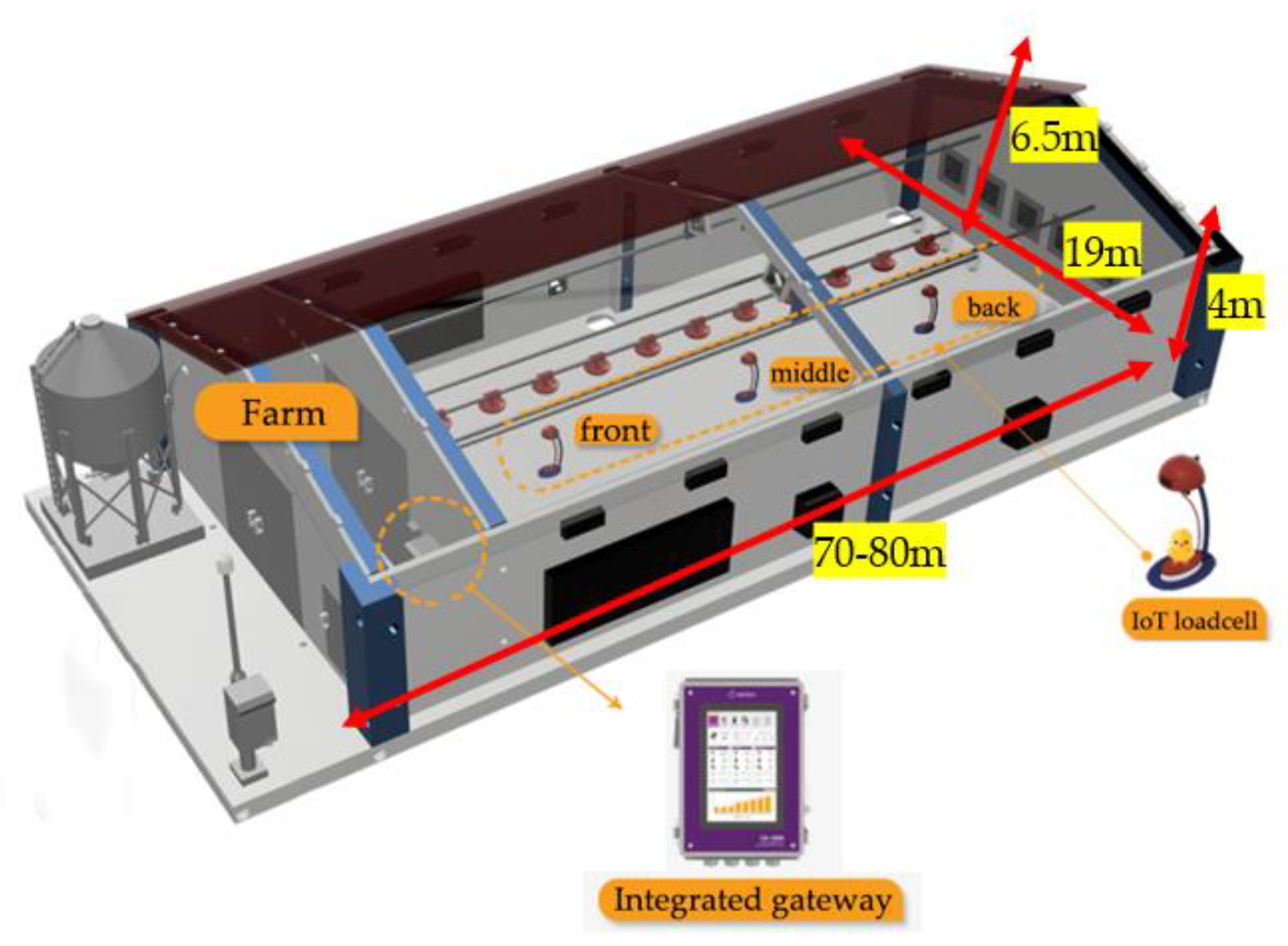
Figure 2.
(a) IoT-enabled weighing sensor devices; (b) synchronized device-captured footage.
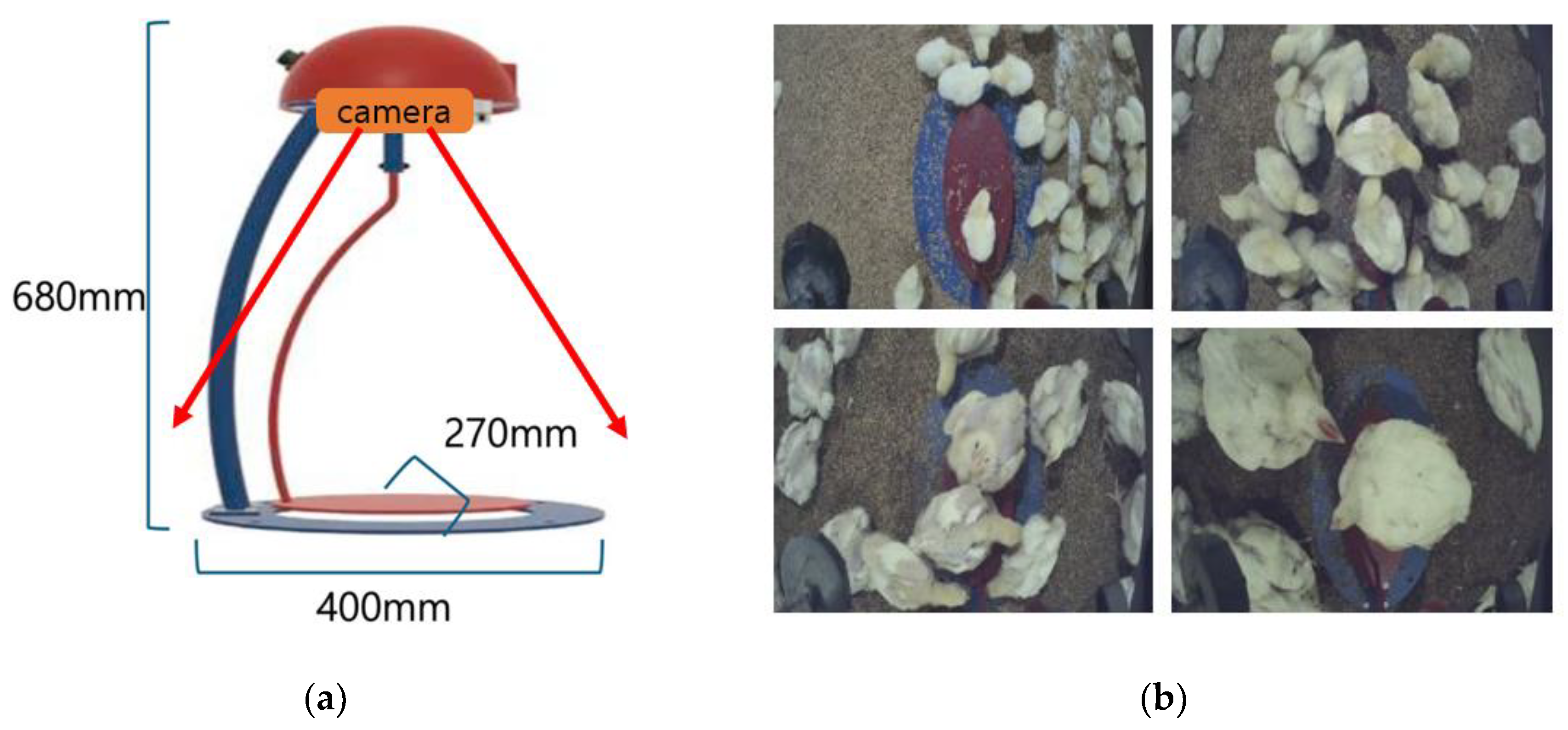
Figure 3.
(a) Composition of the object detection dataset; (b) Number of images in training, validation and test sets.
Figure 3.
(a) Composition of the object detection dataset; (b) Number of images in training, validation and test sets.
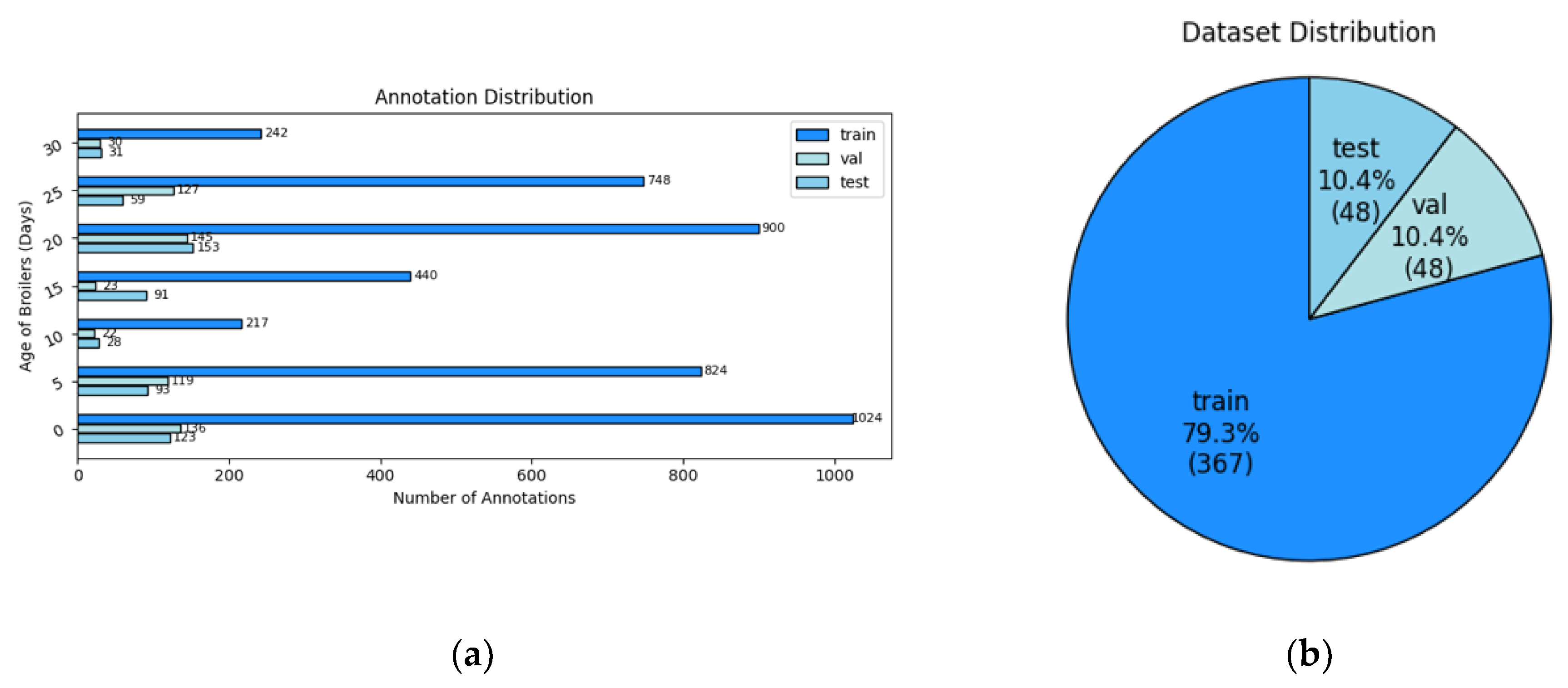
Figure 4.
Algorithm design and implementation.
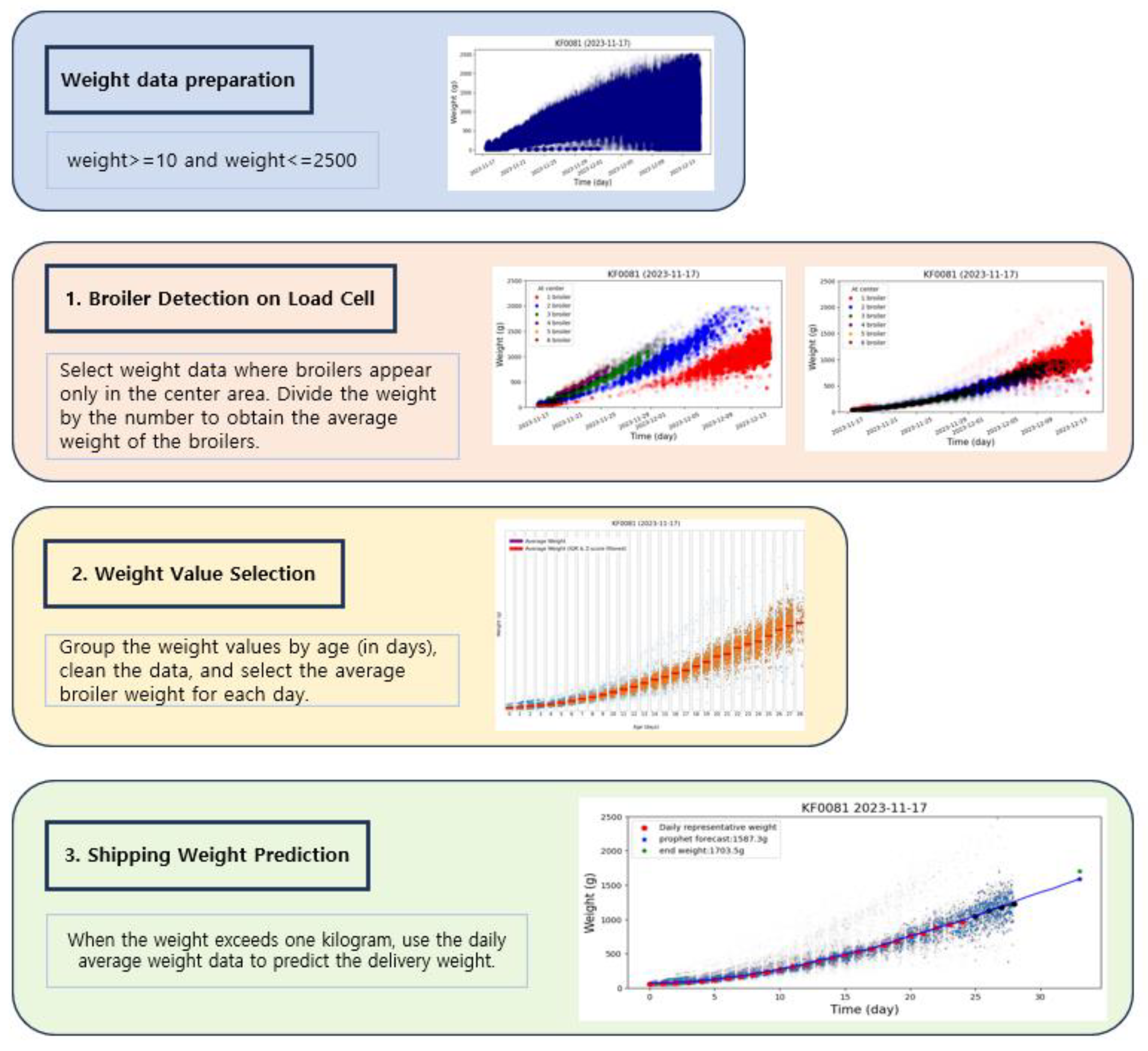
Figure 5.
(a) Experiment A (Basic Configuration); (b) Experiment B (Center Contraction); (c) Experiment C (Edge Expansion).
Figure 5.
(a) Experiment A (Basic Configuration); (b) Experiment B (Center Contraction); (c) Experiment C (Edge Expansion).
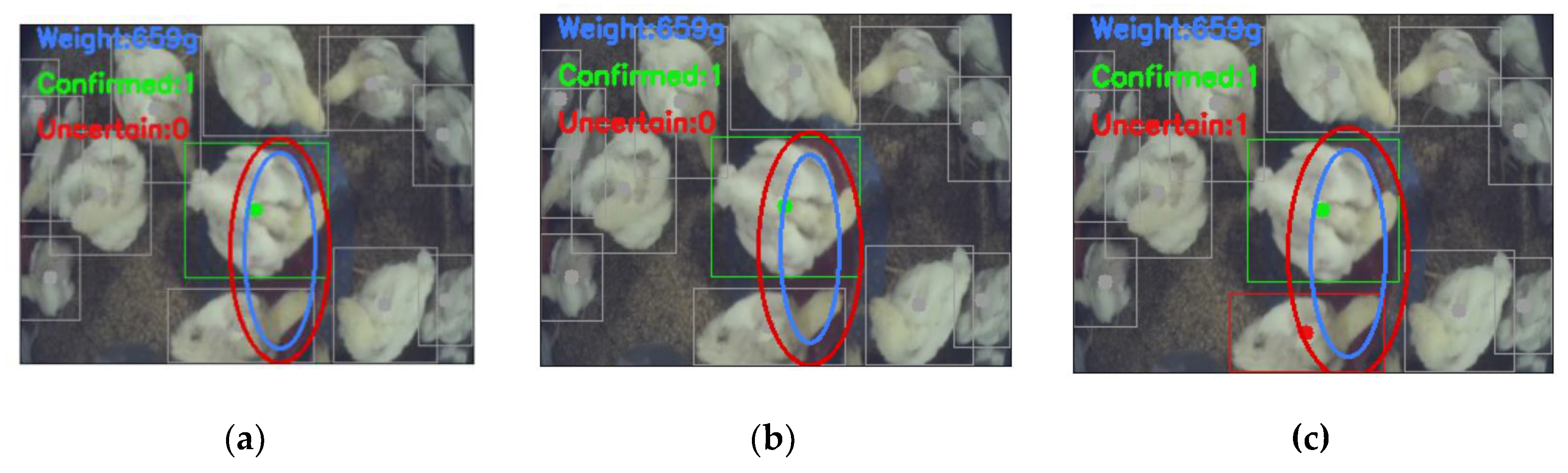
Figure 6.
Comparative performance of various outlier detection methods in shipment weight prediction.
Figure 6.
Comparative performance of various outlier detection methods in shipment weight prediction.
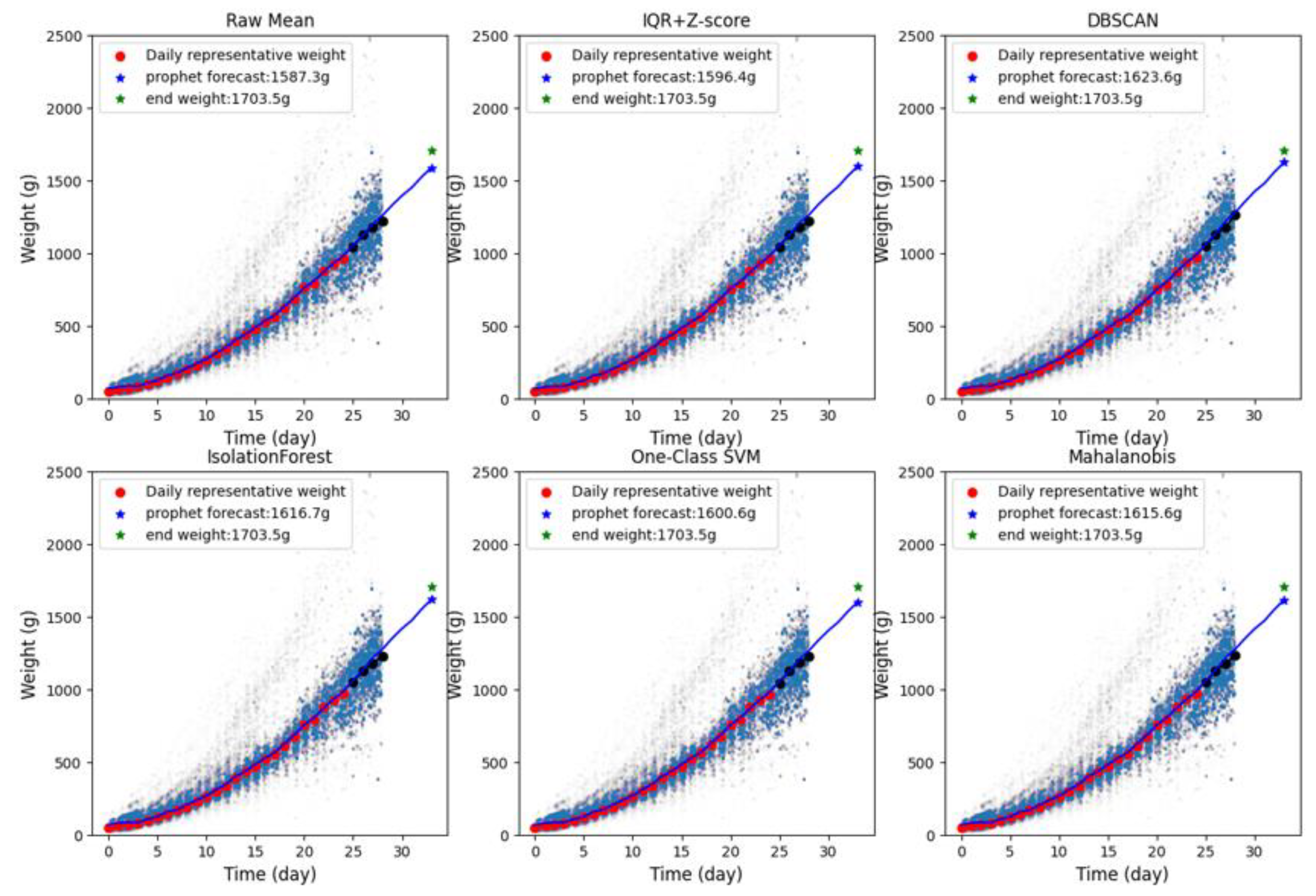
Figure 7.
Performance metrics of the YOLOv8n model during training.
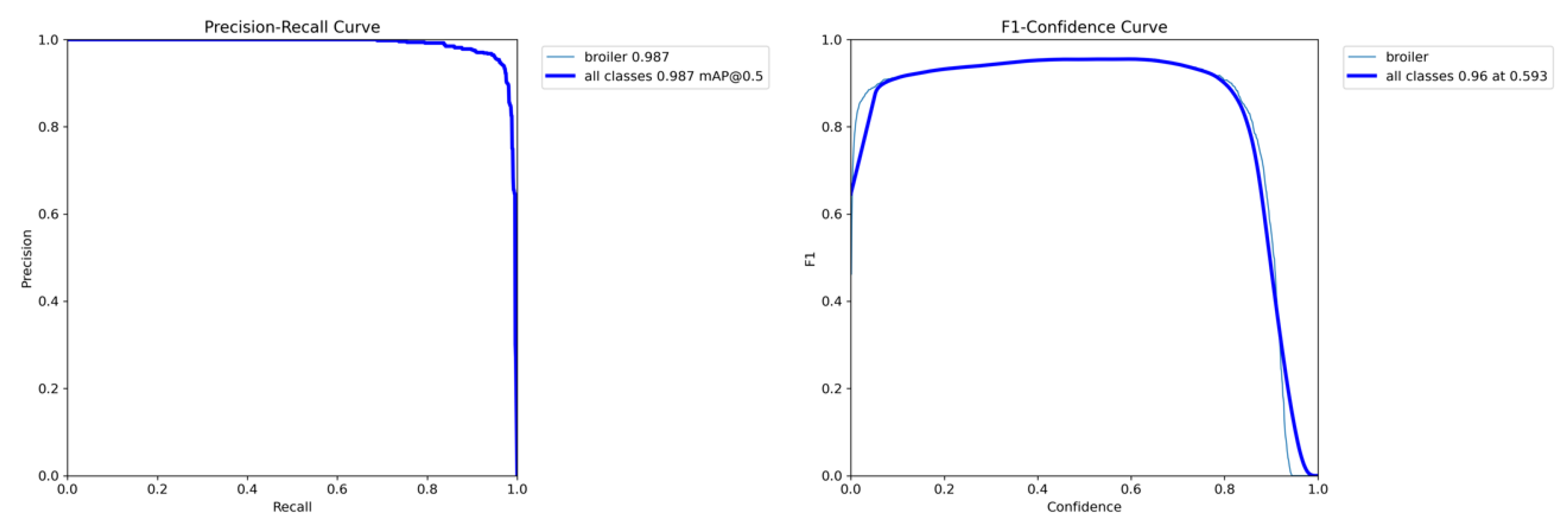
Figure 8.
Results of manual validation for object detection-based broiler counting on weighing platforms.
Figure 8.
Results of manual validation for object detection-based broiler counting on weighing platforms.
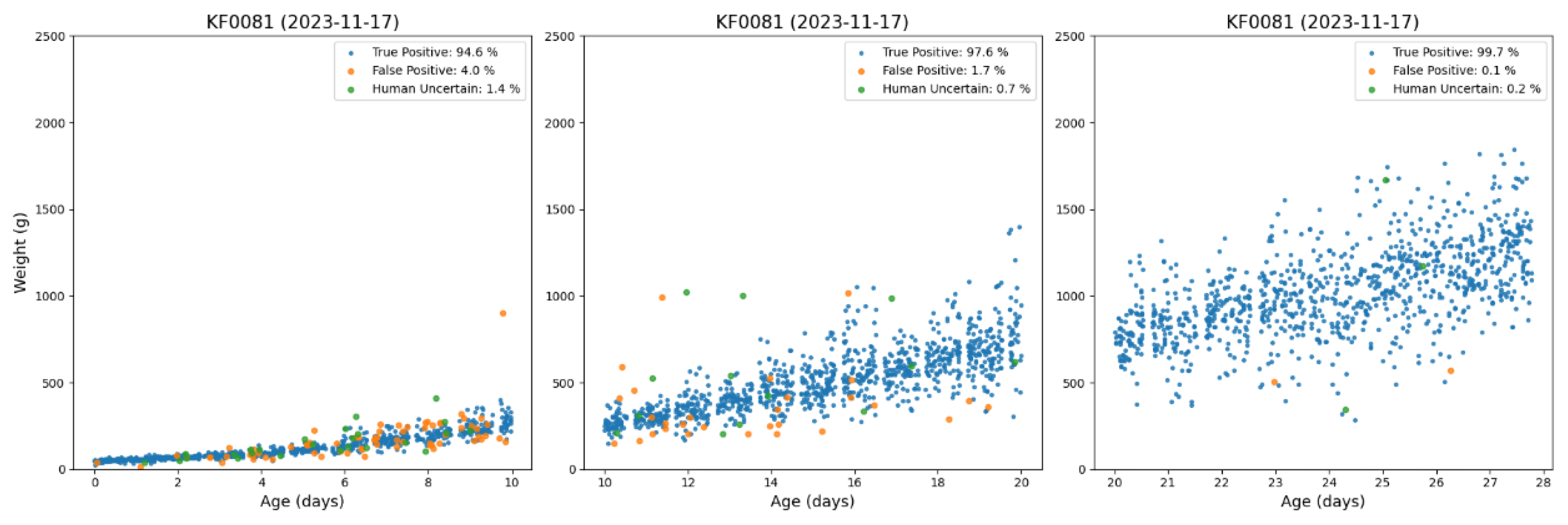
Figure 9.
(a) Detection of 1 broiler on the weighing platform, with red points showing weight distribution when 1 broiler appears in the edge region; (b) Detection of 2 broilers on the weighing platform, with red points representing weight distribution when the total count (central + edge regions) equals 2 and at least 1 broiler appears in the edge region; (c) Detection of 3 broilers on the weighing platform, with red points showing weight distribution when the total count equals 3 and at least 1 broiler appears in the edge region. Green points display average weight distribution when broilers appear exclusively in the central region.
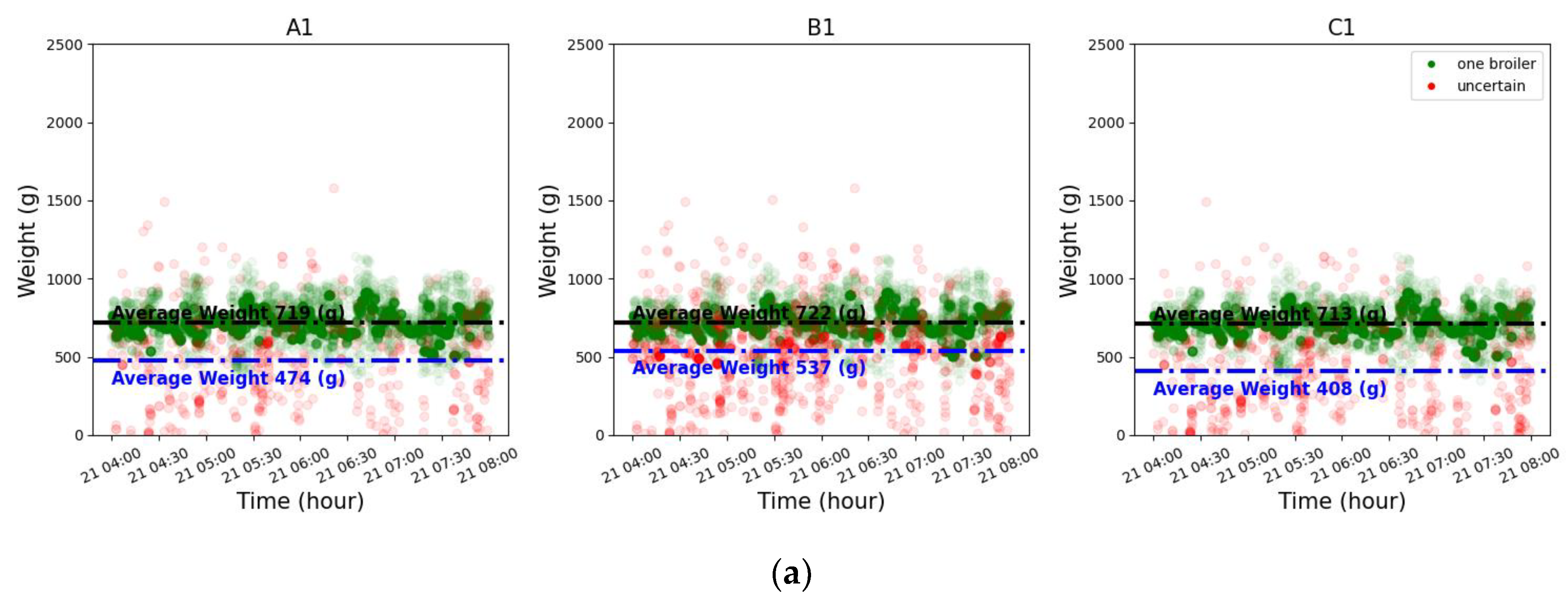
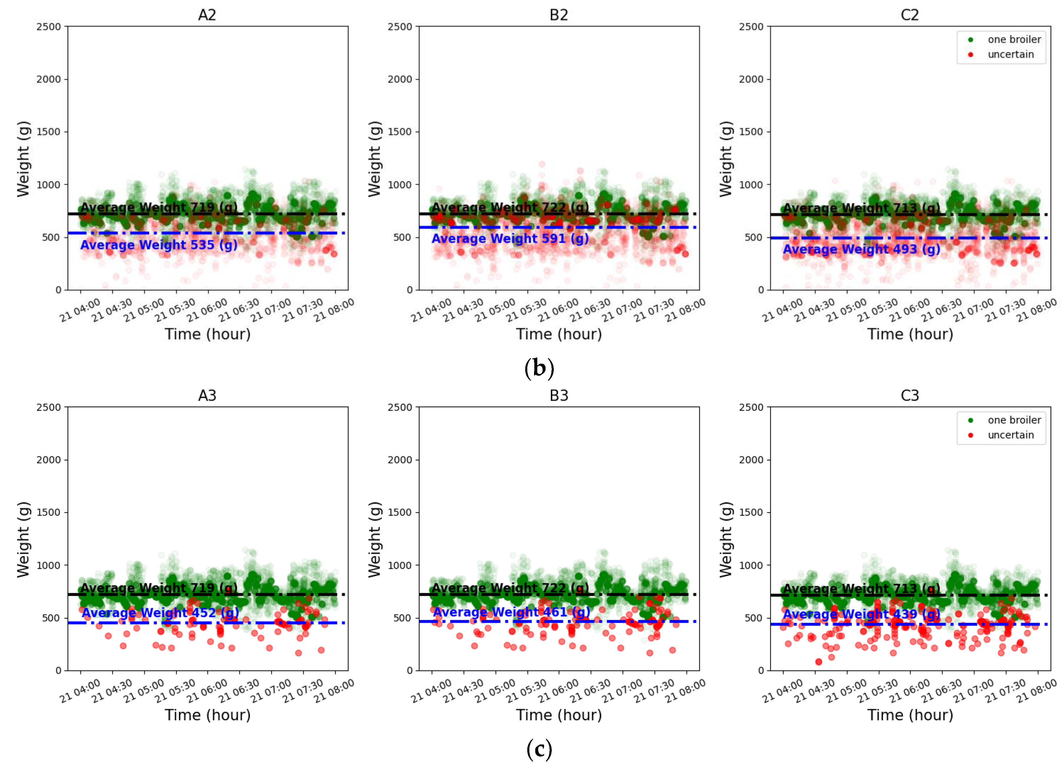
Figure 10.
(a) Distribution of raw weight data; (b) Weight distribution categorized by detected broiler counts; (c) Distribution of individual broiler weights obtained by dividing total weight by broiler count.
Figure 10.
(a) Distribution of raw weight data; (b) Weight distribution categorized by detected broiler counts; (c) Distribution of individual broiler weights obtained by dividing total weight by broiler count.
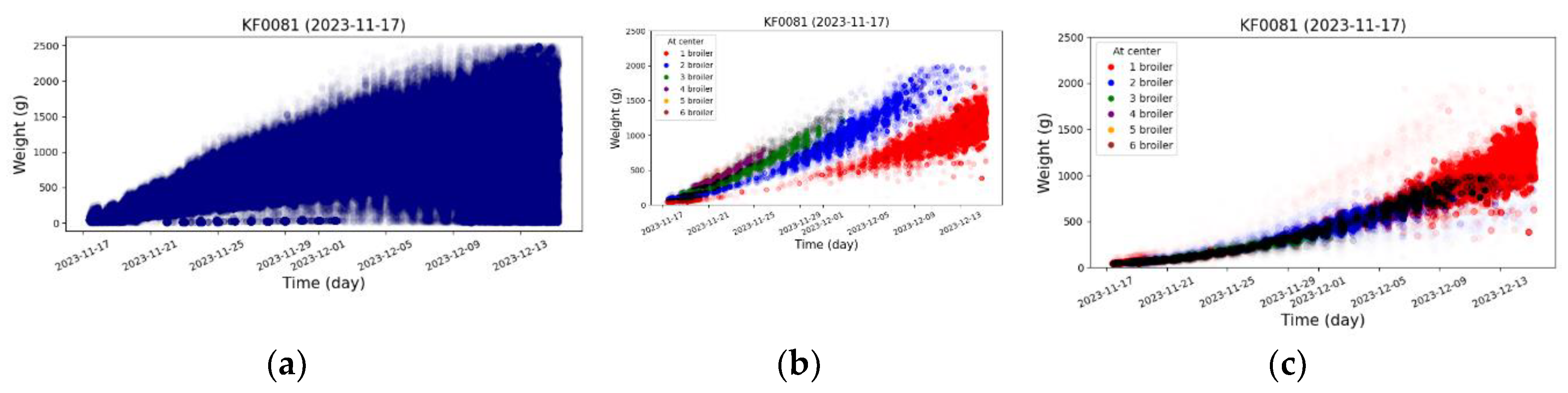
Figure 11.
Comparative effectiveness of different outlier detection methods at 7 days of age.
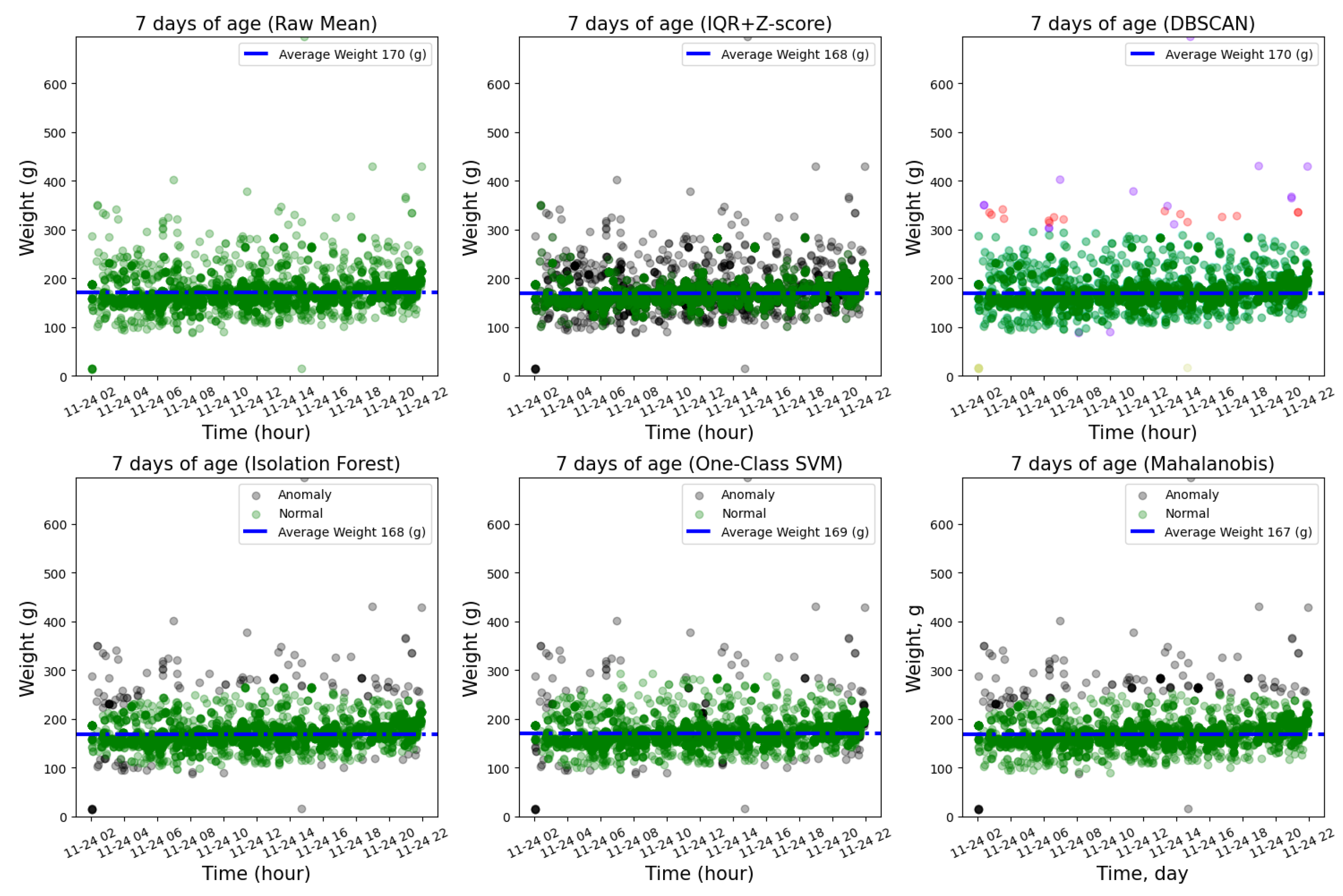
Figure 12.
Representative daily weights by age for dataset 2023_1117_KF0081_01-Img_Data.
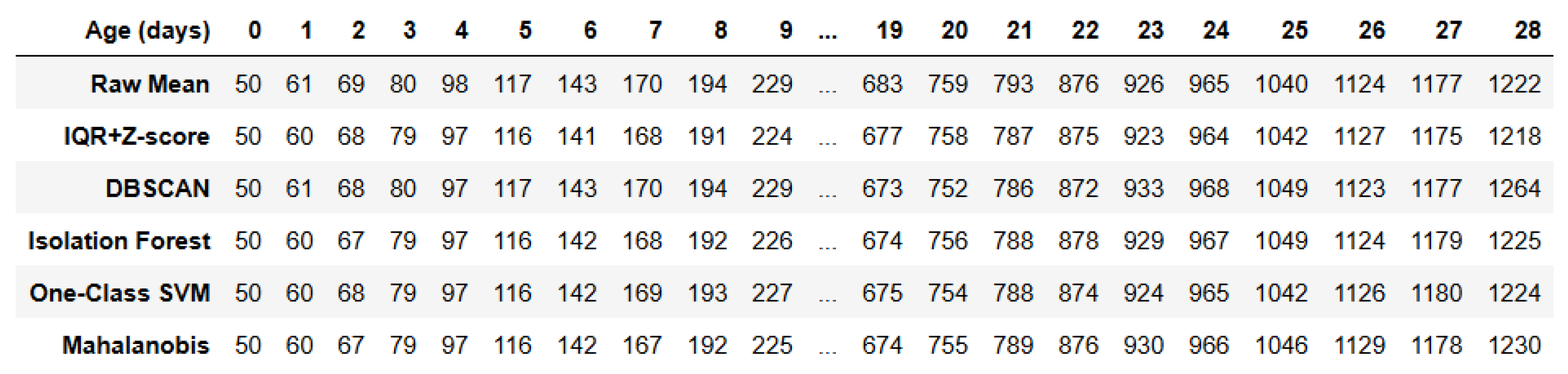
Figure 13.
Daily representative broiler weights obtained by density-based methods (K-means and KDE) in previous studies versus the proposed method in this research.
Figure 13.
Daily representative broiler weights obtained by density-based methods (K-means and KDE) in previous studies versus the proposed method in this research.
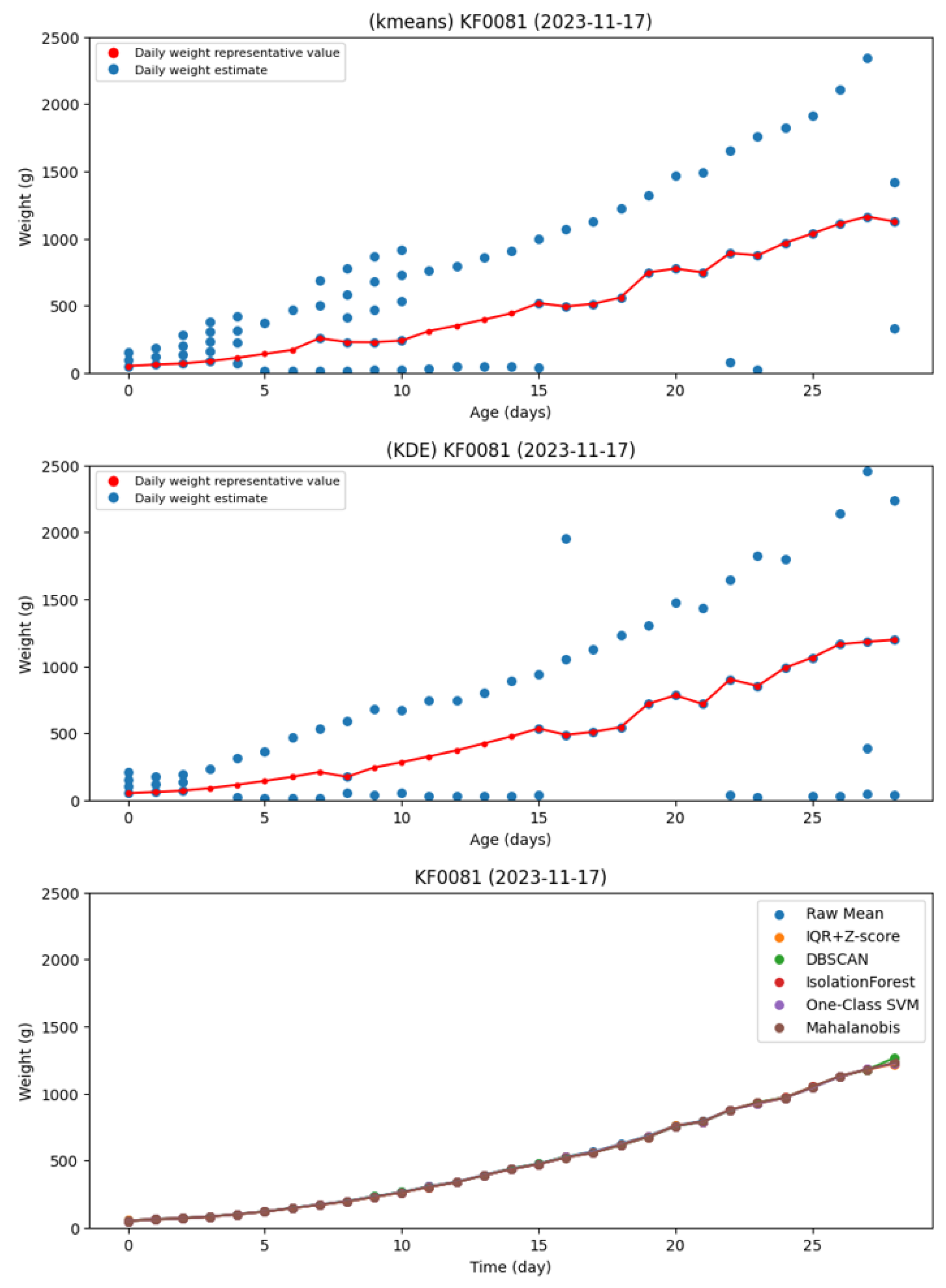

Table 1.
List of the data sets used.
| File Name | Start Date | Delivery Date | Avg. Weight (g) | Images |
|---|---|---|---|---|
| 2023_1117_KF0081_01-Img_Data | 2023-11-17 9:13 | 2023-12-21 7:59 | 1703.5 | 2191039 |
| 2024_0105_KF0081_01-Img_Data | 2024-01-05 11:30 | 2024-02-08 3:59 | 1810 | 2745771 |
| 2024_0502_KF0081_01-Img_Data | 2024-05-02 10:09 | 2024-06-06 23:45 | 1910 | 2589510 |
| 2024_0502_KF0081_02-Img_Data | 2024-05-02 10:09 | 2024-06-06 23:45 | 1910 | 2461297 |
| 2024_1226_KF0081_01-Img_Data | 2024-12-26 11:04 | 2025-01-24 19:59 | 1366 | 2030085 |
Table 2.
Image count by age group.
| Age (days) | 0 | 4 | 8 | 12 | 16 | 20 | 24 | 28 | 32 |
|---|---|---|---|---|---|---|---|---|---|
| train | 69 | 36 | 15 | 16 | 36 | 67 | 72 | 37 | 19 |
| val | 8 | 5 | 2 | 2 | 2 | 12 | 10 | 4 | 3 |
| test | 8 | 5 | 1 | 2 | 7 | 12 | 6 | 4 | 3 |
Table 3.
Experimental environment.
| Equipment | Model |
|---|---|
| Processor | Intel Xeon Gold 5218R CPU Processor NVidia a100-pcie-80gb |
| RAM | 256 GB |
| SSD | 6 TB |
| OS | Ubuntu 20.04 LTS |
Table 4.
List of the data sets used.
| Method | MAE (g) | MAPE (%) | RMSE (g) |
|---|---|---|---|
| k-means | 94.94 | 5.25% | 154.28 |
| KDE | 117.36 | 6.66% | 152.44 |
| Raw Mean | 51.72 | 2.99% | 61.95 |
| IQR + Z-score | 50.6 | 2.92% | 58.72 |
| DBSCAN | 44.36 | 2.56% | 47.97 |
| Isolation Forest | 43.22 | 2.49% | 48.78 |
| One-Class SVM | 46.38 | 2.70% | 54.67 |
| Mahalanobis | 41.82 | 2.43% | 47.88 |
Disclaimer/Publisher’s Note: The statements, opinions and data contained in all publications are solely those of the individual author(s) and contributor(s) and not of MDPI and/or the editor(s). MDPI and/or the editor(s) disclaim responsibility for any injury to people or property resulting from any ideas, methods, instructions or products referred to in the content. |
© 2025 by the authors. Licensee MDPI, Basel, Switzerland. This article is an open access article distributed under the terms and conditions of the Creative Commons Attribution (CC BY) license (https://creativecommons.org/licenses/by/4.0/).
Copyright: This open access article is published under a Creative Commons CC BY 4.0 license, which permit the free download, distribution, and reuse, provided that the author and preprint are cited in any reuse.


