Submitted:
17 July 2025
Posted:
18 July 2025
You are already at the latest version
Abstract
Baroclinic wave resonance, particularly Rossby waves, has attracted great interest in ocean and atmospheric physics since the 1950s. Research on Rossby wave resonance co-vers a wide variety of phenomena that can be unified when focusing on quasi-stationary Rossby waves traveling at the interface of two stratified fluids. This assumes a clear dif-ferentiation of the pycnocline where the density varies strongly vertically. In the atmos-phere, such stationary Rossby waves are observable at the tropopause, at the interface be-tween the polar jet and the ascending air column at the meeting of the polar and Ferrel cell circulation or between the subtropical jet and the descending air column at the meeting of the Ferrel and Hadley cell circulation. The movement of these air columns varies accord-ing to the declination of the Sun. In the oceans, quasi-stationary Rossby waves are ob-servable in the tropics, at mid-latitudes, and around the subtropical gyres (i.e. the gyral Rossby waves GRWs) due to the buoyant properties of warm waters originating from tropical oceans, transported to high latitudes by western boundary currents. The thermo-cline oscillation results from solar irradiance variations induced by the Sun's declination, as well as solar and orbital cycles. It is governed by the forced, linear, inviscid shallow water equations on the β-plane (or β-cone for GRWs), namely the momentum, continuity and potential vorticity equations. The coupling of multi-frequency wave systems occurs in exchange zones. Here, the geostrophic forces reflecting the superposition of zonal/polar and meridional/radial currents of the waves perturb the geo-strophic balance of the basin. Here, it is shown that the ubiquity of resonant forcing in (sub)harmonic modes of Rossby waves in stratified media results from two properties: 1) the natural period of Rossby wave systems tunes to the forcing period - 2) the restoring forces between the different multi-frequency Rossby waves assimilated to inertial Caldirola-Kanai (CK) oscillators are all the stronger as the perturbations of the geostrophic equilibrium in the exchange zones are more significant. According to the CK equations, this resonance mode ensures the sustainability of the wave systems despite the variability of the forcing periods. The reso-nant forcing of quasi-stationary Rossby waves is at the origin of climate variations as well-known as El Niño, glacial-interglacial cycles or extreme events generated by cold drops or, conversely, heat waves. This approach attempts to provide some new avenues for addressing climate and weather issues. Some of these aim to better account for the cli-mate's response to anthropogenic warming.
Keywords:
rossby waves
; eesonant forcing
; tropopause
; subtropical gyres
; tropical oceans
; El Niño
; glacial cycles
; extreme rain and heat events
1. Introduction
Baroclinic wave resonance, particularly Rossby waves, has attracted great interest in ocean and atmospheric physics since the 1950s. Some work focuses on the resonant forcing of atmospheric and oceanic Rossby waves, sometimes leading to the observation of harmonics.
1.1. Atmospheric Rossby Waves
Planetary-scale, westward-traveling waves with discrete periods between 4 and 20 days have been frequently observed in geopotential height and wind fields since the 1950s [1]. These Rossby waves have been identified with various normal modes up to the stratopause at approximately 50 km [2,3,4,5]. Evidence for the existence of large-scale (zonal wave numbers 1, 2, and 3) traveling Rossby waves, has been published [6,7,8]. Further investigations were undertaken for the region up to the mesopause with the aid of Upper Atmosphere Research Satellite Improved Stratosphere and Mesospheric Sounder observations. It was found that wave structures are influenced in the mesosphere by nonuniform and strong background zonal winds and an increasing damping effect with height [9].
More recently, signatures of two transient waves at periods of 16 and 8 days in the middle atmosphere were diagnosed, using meteor-radar wind observations. Their temporal evolution, frequency and wavenumber relations, and phase couplings demonstrated that the 16-day signature is an atmospheric manifestation of a Rossby wave normal mode, and its second harmonic generation gives rise to the 8-day signature, confirming the Rossby wave nonlinearity [10].
The meteorological impact of Rossby wave packets has been studied in both hemispheres. In the Northern Hemisphere, recurrence of transient Rossby wave packets over periods of days to weeks, may repeatedly create similar weather conditions. This recurrence leads to persistent surface anomalies and high-impact weather events. Persistent heatwaves are also observed in the Southern Hemisphere. The relationship between the recurrence of transient Rossby wave packets, atmospheric blocking, amplified quasi-stationary Rossby waves and quasi-resonant amplification was investigated in Southeast Australia [11].
1.2. Oceanic Rossby Waves
1.2.1. The Indian Ocean
The first-baroclinic mode Rossby wave is known to be of critical importance to the annual sea level variability in the southern tropical Indian Ocean. An analysis of continuously stratified linear ocean model reveals that the second-baroclinic mode also has significant contribution to the annual sea level variability [12,13,14]. Studies have investigated how second-baroclinic-mode Kelvin and Rossby waves in the equatorial Indian Ocean interact to form basin resonances at the 180- and 90-day periods. The 90-day resonance happens because the westward-traveling Rossby wave is slower and thus is damped more than the eastward-traveling Kelvin wave [12]. The magnitudes of the second-baroclinic waves are much larger than those of the first-baroclinic waves, because of the larger wind stress projected onto the second-baroclinic mode and the near resonant forcing of the second-baroclinic mode [15,16,17].
It is found that the alongshore winds along the east coast of Africa and the Rossby waves in the off-equatorial areas contribute significantly to the annual harmonics of the equatorial Kelvin waves at the western boundary. The semi-annual harmonics of the Kelvin waves, on the other hand, originate primarily from a linear reflection of the equatorial Rossby waves [18].
Wyrtki jets (which are strong equatorial zonal flows that occur typically during boreal spring and fall in the Indian Ocean) are primarily forced by the semi-annual winds over the equatorial area and a resonant excitation of the second-baroclinic mode has been suggested [17,19,20]. The study of Han et al. [17] has demonstrated that the reflected Rossby waves from the eastern boundary play an important role in the strength and structure of the Wyrtki jets. The reflections of equatorial waves at the meridional and eastern boundaries contribute to the resonant response to wind forcing [21].
1.2.2. The Pacific Ocean
White et al. [22,23] highlighted the resonant response of interannual baroclinic Rossby waves to wind forcing in the eastern mid-latitude North Pacific; Graham et al. [24] found that most of the magnitude in this wave activity occurred in response to wind stress curl forcing in the central and western tropical Pacific, amplified by resonant forcing.
The quasi-decadal oscillation of 9- to 13-year period in the Earth’s climate system has been found governed by a delayed action oscillator mechanism in the tropical Pacific Ocean similar to that governing the El Niño–Southern Oscillation (ENSO) of 3- to 5-year period. It fluctuated in phase with the 11-year-period signal in the Sun’s total irradiance throughout the twentieth century. This association could be explained thanks to the Fast Ocean Atmosphere Model of Jacob et al. [25], in the presence of the 11-year-period solar forcing [26].
The ability of longwave low-frequency basin modes to be resonantly excited depends on how efficiently energy conducted to the western boundary can be retransmitted to the eastern boundary. Explicit calculations of the eigenmodes for a basin geometry similar to that of the North Pacific yield basin modes that are sufficiently weakly damped to be resonantly excited [27].
There is growing evidence that Pacific interdecadal variability contains three spectral resonances the period of which are decadal (13 ± 1-year), bi-decadal (20 ± 5-year) and penta-decadal (60 ± 10-year) [28]. Unlike the bi-decadal resonance, which results from local atmosphere-ocean coupling in the extra-tropics, the penta-decadal and possibly also decadal resonances result from atmospheric and oceanic teleconnections between the extra-tropics and tropics.
1.3. Conditions for Resonant Forcing
Standing equatorial wave modes are shown to be exact solutions of the forced, linear, inviscid shallow water equations when the forcing is zonally uniform and at a single frequency [29]. If the forcing is equatorially confined in the meridional direction, then so is the directly forced response and the standing mode does not leak energy away from the equator. It is shown that some of the solutions of Cane and Sarachik [30] are simplified low frequency forced standing modes.
The spectrum of linear free modes of a reduced-gravity ocean in a closed basin with weak dissipation has been examined [31]. The constraint of total mass conservation, which in the quasi-geostrophic formulation determines the pressure on the boundary as a function of time, allows the existence of selected large-scale, low-frequency basin modes that are very weakly damped in the presence of dissipation. These weakly damped modes can be quasi-resonantly excited by time-dependent forcing near the natural periods, or during the process of adjustment to Sverdrup balance with a steady wind from arbitrary initial conditions. In both cases the frequency of the oscillations is a multiple of 2 /t0, where t0 is the long Rossby wave transit time, which is of the order of decades for midlatitude, large-scale basins. These oscillatory modes are missed when the global mass conservation constraint is overlooked.
For basins with a large variation of the Coriolis parameter, large-scale eigenmodes emerge: the natural frequencies are integer multiples of the frequency for the gravest mode, which, in turn, has a period given by the travel time of the slowest long Rossby wave. The e-folding decay times are comparable to the period and independent of friction. These eigenmodes are excited by stochastic wind forcing and this leads to a weak peak in the spectral response near the frequency of the least damped eigenmode [32]. This decadal-frequency peak is most evident on the eastern and western boundaries and in the equatorial region of the basin.
In a closed basin, the quasi-geostrophic analysis of Cessi and Primeau [31] has shown that weakly dissipated basin modes can be resonantly excited at decadal frequencies. The existence of free basin modes suggests the possibility of spectral peaks, associated with basin-wide resonances, and nontrivial spatial response patterns.
1.4. Resonant Forcing of Quasi-Stationary Rossby Waves
Research on Rossby wave resonance covers a wide variety of phenomena that are difficult to unify. However, this goal can be achieved when focusing on a specific class of Rossby waves. These are the stationary Rossby waves traveling at the interface of two stratified fluids. This assumes a clear differentiation of the pycnocline where the density varies strongly vertically, which is observed both in the atmosphere and in the oceans: 1) In the atmosphere, quasi-stationary Rossby waves are observable at the tropopause, at the interface between the polar jet and the ascending air column at the meeting of the polar and Ferrel cell circulation or between the subtropical jet and the descending air column at the meeting of the Ferrel and Hadley cell circulation. The movement of these air columns varies according to the declination of the Sun [35,36] - 2) In the oceans, quasi-stationary Rossby waves are observable in the tropics, at mid-latitudes, and around the subtropical gyres. They are sensitive to variations in solar irradiance that induce a vertical movement of the pycnocline, which most of the time coincides with the thermocline. The oscillation of this interface in stratified media occurs either as a direct result of the heating/cooling of the water floating above the deep cold waters, or as an indirect effect via winds. Equatorially trapped Rossby and Kelvin waves, as well as off-equatorial Rossby waves, are observed in tropical oceans. They result from the vertical movement of the main pycnocline at the interface between cold deep water and buoyant warm water. Rossby waves are also observed at mid-latitudes, where western boundary currents leave the continents to re-enter the subtropical gyres, as well as very long-wavelength Gyral Rossby waves (GRWs) around the subtropical gyres. The pycnocline is well differentiated around the gyre due to the buoyant properties of warm waters originating from tropical oceans, transported to high latitudes by western boundary currents.
Quasi-stationary long-period Rossby waves are responsible for climate variations as familiar as El Niño, glacial-interglacial cycles, or extreme events generated by cold drops or, conversely, heat waves. These climatic phenomena, however varied they may be, result from the resonant forcing of these Rossby waves due to variations in solar irradiance.
2. Materials and Methods
2.1. Data
The daily Ocean Surface Current Analyses Real-time (OSCAR) Surface Currents - Final (0.25◦ × 0.25◦) since 1993 (Version 2.0) are provided by the National Aeronautics and Space Administration (NASA) [37,38].
The wind velocity as a function of atmospheric pressure (17 levels) is obtained from the NCEP/DOE Reanalysis II data provided by the National Oceanic and Atmospheric Administration (NOAA) PSL, Boulder, CO, USA. The daily gridded data (2.5◦ × 2.5◦) from 1979 to now [39] are available at https://www.psl.noaa.gov/data/gridded/data.ncep.reanalysis2.html, accessed on 13 May 2024.
2.2. In Search of a Unified Explanation of Resonant Forcing of Quasi-Stationary Rossby Waves
Whether oceanic or atmospheric Rossby waves, their forcing becomes all the more significant when the natural period of oscillation of the interface is close to the period of forcing. This resonant forcing promotes the interface oscillation because Rossby waves behaving like inertial oscillators, the synchronism between the forcing and the wave response causes the amplitude to increase during each period until Rayleigh friction limits this growth. When this synchronism is lacking, the forcing irremediably opposes the movement of the interface, which causes the damping of asynchronous waves. The coincidence of the forcing period and the natural period of the Rossby wave may seem fortuitous because, since long-period Rossby waves are approximately non-dispersive, their apparent wavelength must adjust so that the two periods tune. This apparent wavelength is perceived by a fixed observer: westward-traveling, Rossby waves are generally embedded in an eastward-traveling baseflow.
Traveling at the interfaces of stratified media, Rossby waves owe their origin to the gradient β of the Coriolis frequency relative to the latitude. In cartesian coordinates, the forced, linear, inviscid shallow water equations on the β plane are momentum equations (1), (2) and the continuity equation (3), with the potential vorticity equation (4) that follows from the previous ones (surface stress is not considered) [35,42]:
where is the perturbation of the interface height , u is the zonal current, v the meridional current; is the thickness of the upper layer, where is the Coriolis frequency, and the acceleration of gravity. is the relative vorticity. The forcing term is the ascending/descending velocity of the interface under the effect of solar irradiation.
This system of equations of motion concerns tropospheric quasi-stationary waves as well as off-equatorial and equatorial oceanic quasi-stationary waves to which equatorial Kelvin waves should be added: since equations (1) and (3) give , .
The dispersion relation is, in the case of long planetary waves, approximated by:
where c is the phase velocity of Rossby waves along the equator. ω/k is the phase velocity of Rossby waves at latitude φ, ω is the pulsation, and k the wave number, Ω is the rotation rate of the Earth, R is the radius of the Earth.
On the other hand, as regards very long period GRWs winding around the subtropical gyres, the β plane approximation has to be replaced by the β cone approximation so that GRWs owe their origin to the gradient β of the Coriolis frequency relative to the mean radius of the gyre [43]. The dispersion relation is virtualy the same as (5) where φ represents the latitude of the gyre’s centroid.
In all cases, the solution of this system of equations involves the vertical perturbation η of the interface as well as the zonal current u and meridional current v. They depend on the time t as well as the cartesian or conic coordinates depending on whether the β-plane or the β-cone approximation is used. These quasi-periodic terms are such that the meridional/radial current v is in phase with the forcing term E while the vertical perturbation η of the interface and the zonal/polar current u are in quadrature.
2.3. Resonant Forcing in Harmonic and Subharmonic Modes
Rossby waves form multi-frequency coupled wave systems. Indeed, when the forcing results from the declination of the Sun, the fundamental wave system, with an annual period, produces wave systems with shorter periods, which can be seasonal. In the case of orbital forcing of GRWs, these may reflect the cycles of the different orbital parameters, precession, obliquity, and eccentricity. The coupling of superimposed multi-frequency wave systems occurs in exchange zones. Here, the geostrophic forces reflecting the superposition of zonal/polar and meridional/radial currents of the waves perturb the geostrophic balance of the basin. In the absence of forcing, the motions of the wave system tend to become quasi-geostrophic. This acts as a restoring force. The conditions for the sustainability of such dynamic systems require that each oscillator receives as much interaction energy from other oscillators as it gives them overtime. It can be described by the Caldirola-Kanai equations, which are a prototype of coupled oscillator systems. This governs the motion of a system of N coupled oscillators with inertia corresponding to the N resonance frequencies. Applied to the case of multi-frequency forced Rossby wave systems, it gives [44]:
where is the phase of the ith oscillator, here the modulated geostrophic zonal/polar current , the inertia parameter, here the mass of water displaced during a cycle resulting from the quasi-geostrophic motion of the ith oscillator, the damping parameter referring to the Rayleigh friction and measures the coupling strength between the oscillators and . The right-hand side describes the periodic forcing with frequency where is the amplitude of the forcing on the oscillator. The restoring force simply depends on the phase difference between the oscillators. So, it vanishes when the phases are equal so that the geostrophic forces reflecting the superposition of the waves in the exchange zone remain unchanged. On the other hand, the interaction between the oscillators and is all the stronger as the difference in zonal/polar velocities is higher. This is because the geostrophic forces of the exchange zone impact the geostrophic balance of the basin so that the faster current slows down in favor of the slower current which accelerates. In other words, the geostrophic balance of the basin levels the crests and valleys of the velocity field of modulated geostrophic currents resulting from baroclinic waves subject to external forcing.
Multi-frequency Rossby wave systems share common characteristics. They are fed by an input current, have common exchange zones (coupling regions) where the forcing of Rossby waves occurs resonantly, and finally an output current. This process is repeated stationarily. The quasi-periodicity of the motions, which mirror the quasi-periodicity of the forcing, makes Rossby wave systems appear quasi-stationary. The interaction energy of the oscillator, that is the Hamiltonian of the dynamic system (6), is given by [44]:
It is from this relationship that a necessary and sufficient condition to ensure the durability of the resonant oscillatory system is established: the coupled oscillators form oscillatory subsystems so that the resonance conditions are to be defined recursively:
where or 3. Indeed, the resonance of the fundamental wave system implies that its period tunes to the forcing period T, which requires a control mechanism based on a significant phase shift and adjustable through the wave system.
The purpose of this article is to emphasize the characteristics of the different dynamic systems that lead to major climatic variations, in order to better understand and/or better anticipate them. The approach will consist of highlighting - 1) the exchange zones where the coupling of multi-frequency wave systems occurs to produce harmonics and/or subharmonics of the fundamental wave system - 2) the mechanisms leading to the tuning of the periods of the dynamic system to the forcing period.
3. Results and Discussion
3.1. Rossby Waves in the Tropical Oceans
The three tropical oceans form a system of annual waves resonantly forced by the declination of the Sun and the associated easterlies.
3.1.1. The Tropical Pacific
The tropical Pacific Ocean is traversed by a system of strongly coupled Rossby waves, an annual fundamental wave, and two subharmonic waves with mean periods of 4 and 8 years (the biennial wave is not shown). In order to highlight the variability of different wave systems, they are represented in Figure 1 on 15/11/1997 and Figure 2 on 15/12/2006. The dates are chosen so that an El Niño event reached its maturation stage characterized by a thermal anomaly in the eastern equatorial Pacific (EP) event in Figure 1 and in the central equatorial Pacific (CP) event in Figure 2, causing a response of the Walker circulation [45,46].
The amplitude, coherence and phase of Rossby waves are obtained respectively from the square root of the cross-wavelet power, the wavelet coherence and the coherence phase of the current velocity, namely sign where and are the zonal and meridional components of the velocity [47]. The amplitude of the modulated current velocities of the different wave systems is represented in Figure 1a,d,g and Figure 2a,d,g. The coherence (Figure 1b,e,h and Figure 2b,e,h) with respect to the temporal reference located at 0.5°N, 159.5°E shows the consistency of the different components of the wave systems. The phase (Figure 1c,f,i and Figure 2c,f,i) exhibits the time shifts, with respect to the reference, of the wave systems.
- The annual Rossby wave system
Figure 1a–c is obtained by scale-averaging the geostrophic current velocity over the 0.75-1.5 year period range. The annual wave is formed by 4 well-differentiated zonal bands in its eastern part beyond 180°. These 4 bands are in phase opposition two by two. The latitude of the northernmost band is close to 15°N (phase in blue), the two bands on either side of the equator (phase in red and blue) are well separated beyond 150°W, finally the southernmost band (phase in red) is located at latitude 5°S. This suggests that the four coherent bands highlight the first-baroclinic mode, fourth-meridional mode Rossby wave [48]. The modulated geostrophic current of the Rossby wave is rooted deep in the tropical ocean, exhibiting a high meridional mode [49]. These bands tighten in the western part of the basin to form a broad band whose phase is homogeneous. Only the northernmost band remains, reaching the western boundary of the basin. This suggests a change in mode of the Rossby wave in the western part of the basin, to become a first-baroclinic mode, first-meridional mode Rossby wave. What was the northernmost band of the Rossby wave in the eastern part of the basin is no longer an integral part of the Rossby wave in the western part.
The northernmost band constitutes the modulated component of the North Equatorial Current (NEC). The two bands on either side of the equator constitute the modulated components of the North Equatorial Counter Current (NECC) and the northernmost ramification of the South Equatorial Current (SEC). These two modulated currents merge around latitude 160°W, the SEC being retroflected to join the NECC. The southernmost branch, on the other hand, is supported by the southernmost branch of the SEC. Mainly forced by easterlies in boreal winter, the modulated current velocity can reach 0.44 m/s in the northern hemisphere (Figure 1a,c): the phase is close to zero in the western part of the basin, which corresponds to January-February.
The tuning of the natural Rossby wave period to the annual forcing period is done by matching, in the eastern part of the basin, the fourth-meridional mode whose phase velocity is much lower than that of the first-meridional mode: the phase velocity is where ω is the pulsation, k the wavenumber, 2.8 m/s the phase velocity of the first-baroclinic mode Kelvin wave and m the meridional mode of the Rossby wave. Consequently, the phase velocity of the fourth-meridional mode Rossby wave is 3 times lower than that of the first-meridional mode Rossby wave. The change in the meridional mode of the Rossby wave around 160°W means that its natural period is annual (the first-meridional mode Rossby wave takes 6 months to cross the Pacific Ocean, the fourth-meridional mode Rossby wave takes 18 months). As shown in Figure 2, the longitude where the meridional mode changes varies significantly depending on the year: it is about 180° on 15/12/2006, which constitutes a tuning factor for the natural period of the annual Rossby wave.
- The quadrennial wave system
As shown in Figure 1d–f obtained by scale-averaging the geostrophic current velocity over the 3-6 year period range, the quadrennial wave consists of a main band along the equator, which testifies to the presence of a first-baroclinic mode, first-meridional mode equatorial Rossby wave. The phase difference of the wave between the eastern and western boundaries of the basin is 6-8 months, which corresponds to the traveling time of the equatorial Rossby wave. It is propelled westward by the Southeast Trade Winds to about longitude 180° E (phase in indigo in Figure 1f). Two strongly phase-shifted off-equatorial Rossby waves are visible at latitudes 5°N carried by the NEC and 10-20°S carried by the SEC (phases in light blue), west of the basin up to the longitude 170°W. They are almost 3 years ahead compared to the equatorial wave in its western part.
While the geostrophic current velocity anomaly shows a single equatorial band, the coherence and phase of the equatorial Rossby wave show that it consists of two zonal bands in its eastern part, then approaches and merges in its western part, at about 180° longitude. In its eastern part, the northernmost band merges with the NECC, the southernmost with a branch of the SEC, as do the two in-phase bands of the annual wave, slightly behind the temporal reference (phase in red in Figure 1c).
Due to geostrophic forces acting to the west of the tropical basin, the equatorial Rossby wave is deflected as it approaches Indonesia, and divided towards the north and towards the south, to form the two off-equatorial branches. The phase velocity of off-equatorial Rossby waves is lower the further they move away from the equator, which constitutes a parameter for tuning the period of the quadrennial wave system. Then, after almost 3 years, the off-equatorial waves come back to the equator to form a Kelvin wave (hidden by the equatorial Rossby wave in Figure 1f), thanks to the geostrophic forces acting to the west of the tropical basin. This Kelvin wave will be “reflected” against the South American continent to form an equatorial Rossby wave and the cycle begins again.
The tuning of the quadrennial wave system is carried out owing to its two off-equatorial branches. They behave like the slide of a brass instrument such as the slide trombone. But while the annual wave is resonantly forced by the declination of the Sun and the resulting easterlies, the quadrennial wave is partly forced by the El Niño Southern Oscillation (ENSO), partly by its coupling with the annual wave. ENSO occurs when the Kelvin wave, which causes warm waters to migrate from the west to the east of the tropical basin under geostrophic forces, encounters cold waters off Peru and Chile, promoting strong evaporative processes. This results in a rise of the thermocline, the start of a new 4-year average period cycle that may be accompanied by an El Niña event when upwelling off the coast is stimulated under the effect of recession of the Rossby wave and resulting geostrophic forces. Nevertheless, this forcing mode causes the quadrennial wave period to undergo considerable variability, with two consecutive ENSO events that may be separated by 1.5 to 7 years.
In Figure 2d–f the geostrophic current velocity anomaly is much lower than in the previous case, the coherence of equatorial and off-equatorial current velocities as well. Off-equatorial currents are identifiable by the phase in yellow 5°N, in light blue 20°S (Figure 2f), which confirms the durability of the role played by the modulated components of the NECC and the SEC in the tuning of the period of the quadrennial wave system.
- The 8-year period wave system
Although the geostrophic current velocity anomaly is low, except in the western part of the basin, the 8-year period wave system looks similar to the previous one when a change in the period scale is made (Figure 1g–i and Figure 2g–i). Thus, it contributes to ENSO due to the transfer of warm water from the western to the eastern Pacific by the Kelvin wave. Here again, the tuning of the natural period is carried out thanks to off-equatorial currents which are strongly out of phase in the western part of the basin (phase in light blue in Figure 1i and Figure 2i). But the presence of out-of-phase zonal bands in the eastern part of the basin suggests that several modes coexist.
- Coupling of the wave systems
The exchange zones where the coupling in (sub)harmonic modes of the different wave systems occurs, which are deduced from the temporal and spatial coherence of the main subharmonic pairs, are shown in Figure 1j–l and Figure 2j–l. These sub-figures show extended exchange zones between the 2 main subharmonics and the fundamental annual wave (j, k), as well as the 2 subharmonics between them (l). The surface of the areas involved in coupling is subject to significant variability. The same is true of the interaction forces between the different wave systems. The wave systems observed in November 1997 reveal strong interactions, mainly between the fundamental wave and the two main subharmonics. The couplings are less pronounced in December 2006. However, in both cases, coupling occurs mainly in the western part of the basin, particularly in the area where the SEC is deflected against Indonesia to form the NECC, as well as along the NECC north of the equator and along the SEC south of the equator.
Some properties of ENSO are inherited from the couplings between the 3 main wave systems (here, the harmonic of half a year average period is ignored). ENSO depends on the date of occurrence compared to the central value of 4-year intervals of January 1992 to January 1996, January 1996 to January 2000, etc. (Figure 3). Indeed, the Rossby wave is coherent in its entirely when the lag is close to zero while it undergoes a loss of temporal coherence when the lag increases. This is illustrated by the strength of the coupling between the different harmonics reflected by the efficiency of geostrophic forces in generating ENSO. Figure 1 and Figure 2 represent the geostrophic current velocity anomalies, both at the end of autumn but with different lags, equal to -0.17 and 1.00 years, respectively. In both cases, the equatorial Rossby wave recedes after ENSO occurs, in November 1997 and in December 2006, respectively, but more or less in line with the geostrophic balance of the tropical basin.
From [42] Central Pacific (CP) events always occur while the El Niño peaks out of phase with the annual quasi-stationary wave (segments in red, no event can occur in the black segment). Eastern Pacific (EP) events occur while the El Niño peaks in phase with the annual quasi-stationary wave (green, dark, and light blue segments). This speciation of ENSO according to its date of occurrence is attributable to the interactions between the geostrophic forces of the exchange zones and the geostrophic balance of the tropical basin. The distinction between CP and EP events, which depends on the synchronization between the annual and quadrennial wave systems, reflects the role of the phase shift between the Kelvin waves produced by these two wave systems. The volume of warm water transferred from the west to the east of the equatorial Pacific depends on this.
Figure 4 helps to elucidate the role played by the 8-year average period wave system on ENSO. The coupling of the two subharmonics causes ENSO to produce three events in four years close to the maximum amplitude of the power spectrum of the wave system in the western part of the basin (0.5°N, 159.5°E), due to the width of the peak.
3.1.2. The Tropical Atlantic
In addition to the annual fundamental wave system, the tropical Atlantic Ocean is crossed by a harmonic wave system with a mean period of half a year (Figure 5) [50].
- The annual wave systems
The phase of the equatorial Rossby wave is anti-symmetrical with respect to the equator, with the two opposite parts being in phase opposition, which characterizes the second-meridional mode of the wave. Its apparent wavelength is close to the distance between the eastern and western boundaries of the basin at the equator, which is evidenced by the anti-symmetry of the phase with respect to the meridian at 10°W. The phase velocity of the first-baroclinic mode, second-meridional mode equatorial Rossby wave is m/s = 0.56 m/s so that the Rossby wave takes almost 4 months to cross the Atlantic. The period is tuned by both the zonal Rossby waves embedded in the South Equatorial Current (SEC) between 10°S-20°S and the North Equatorial countercurrent (NECC) between 5°N-10°N. Off-equatorial waves are out of phase relative to the equatorial Rossby wave west of the basin (phase in light blue in Figure 5c,f).
The dynamics of the annual wave system resembles that of the Pacific quadrennial wave system. Due to geostrophic forces acting to the west of the tropical basin, the equatorial Rossby wave is deflected as it approaches the American continent, and divided towards the north and towards the south, to form the two off-equatorial branches, which constitutes a parameter for tuning the period of the annual wave system. Then, after 6-7 months, the off-equatorial waves come back to the equator to form a Kelvin wave (hidden by the equatorial Rossby wave in Figure 5f), thanks to the geostrophic forces acting to the west of the tropical basin. After about twenty days, the equatorial Kelvin wave forms a poleward coastal wave when it encounters the African continent. This wave then flows back equatorward due to the geostrophic forces of the basin (after a short period, this is hardly noticeable in Figure 5f) to form an equatorial Rossby wave, and the cycle begins again. The annual wave system is forced by easterly winds in the eastern part of the basin up to about 5°W longitude so that surface stress is exerted in the direction of the geostrophic current in both boreal and austral winter.
- The semi-annual wave systems
The two wave systems, annual and semi-annual, are distinguished by the meridional mode of the equatorial Rossby wave. Indeed, in the case of the semi-annual wave, the Atlantic is crossed by a first-baroclinic mode, first-meridional mode Rossby wave attested by the symmetry of the wave with respect to the equator. Moreover, an important difference appears regarding off-equatorial Rossby waves which are much more developed in the case of the annual wave. This partly explains the difference in periods between the two systems, the other part coming from the fact that the Rossby wave of the first-meridian mode is faster than that of the second-meridian mode (2.3 months instead of 3.8 months).
As shown in Figure 5g, wave system coupling occurs in an equatorial exchange zone that extends 25°W to 5°W. The strong temporal and spatial coherence between the two wave systems highlights the strong interaction between the fundamental wave and the main harmonic.
3.1.3. The Tropical Indian Ocean
- The semi-annual wave system
The tropical Indian Ocean is characterized by the superposition of three Rossby wave systems whose mean periods are 1/2-, 1- and 4-years (Figure 6) [51]. Here, the fundamental wave system is semi-annual. This is supported by 1) the velocity of the Equatorial Geostrophic Current, which reaches 0.47 m/s (average velocity of the upper quantile) along a broad ridge, in the period range 0.37-0.75 years (Figure 6a) – 2) the two off-equatorial currents west of the basin, out of phase with the equatorial Rossby wave, and by the phase change between the eastern and western parts of the equatorial Rossby wave, these indices underlining the tuning of the natural period of the wave system to the semi-annual forcing period (Figure 6b,c).
These observations suggest that the equatorial wave is a westward-traveling first-baroclinic, first-meridional mode Rossby wave. It is deflected as it approaches the African continent, and divided towards the north and towards the south, to form the two off-equatorial branches (dark blue phase in the north, light blue in the south). The northernmost current is embedded in the Northeast Monsoon Drift in the Arabian Sea; the southernmost current is embedded in the South Equatorial Current. These off-equatorial Rossby waves reverse a quarter of a period later to reflect against the African continent under the effect of geostrophic forces, giving rise to an eastward-traveling Kelvin wave. However, it appears that the Kelvin wave does not reach the eastern boundary of the basin, in this case Indonesia, but, embedded into the equatorial countercurrent (ECC), flows back as a Rossby wave to longitude 95°E under the effect of geostrophic forces. The forcing results mainly from the surface stress caused by reversing Asian monsoon winds.
- The annual wave system
The dynamics of the annual wave system breaks down as follows: the equatorial Rossby wave is diverted against the African continent in May-June (phase in red) to form off-equatorial Rossby waves that merge with the semi-annual waves (Figure 6e,f). Half a period later, they reverse (phase in blue) and reflect off the African continent to form an eastward-traveling equatorial Kelvin wave, driven by the equatorial countercurrent. This equatorial wave will travel westward as a Rossby wave, as the equatorial countercurrent slows down.
In addition to being a subharmonic wave of the semi-annual wave, the annual wave is influenced by the western Pacific basin through coherent baroclinic waves. This is because the water in the western equatorial Pacific Ocean has a higher temperature and lower salinity than the water in the Indian Ocean. One is embedded in the South Equatorial Current originating from the throughflow from the Timor passage, approaching the equator 8°S, with a half-period phase rotation (first yellow-orange phase, then blue). Further north, another coherent wave is embedded in the current from the Pacific which joins the monsoon current of the Indian Ocean, this time without phase variation (phase in blue). Finally, a strong coherent modulated geostrophic current forms an arc between Malaysia and Kalimantan (phase in orange), lagging behind the equatorial wave by a quarter of a period. This is probably the result of atmospheric coupling between the equatorial Indian Ocean and the far western Pacific, associated with the synchronized variation in sea level resulting from throughflows. A four-year period subharmonic is superimposed on the equatorial wave systems Figure 6g–i.
As shown in Figure 6j–l) the Rossby wave coupling occurs mainly in an equatorial exchange zone located to the west of the basin, between longitudes 50°E and 80°E. It mainly concerns the very strong link between the fundamental and the annual subharmonic, as well as between the fundamental and the 4-yr period subharmonic to the east of Malaysia (Figure 6j).
3.2. Quasi-Stationary Rossby Waves in the Tropopause
3.2.1. The Northern Hemisphere
In Figure 7 the amplitude, coherence and phase of the wind velocity at 250 mb in relation to a temporal reference (the wind velocity at 30°N, 0°E) is represented on 01/01/2002. The mean periods of the main harmonics are 1/128 year (a, b, c), 1/32 year (d, e, f), 1/16 year (g, h, i), 1/8 year (j, k, l), 1 year (m, n, o), and 2 years (p, q, r). The velocity of the modulated airflows varies a lot according to the harmonics (Figure 7a,d,g,j,m,p). On the other hand, one of the peculiarities of Rossby waves at the tropopause is that they are coherent over a large area as shown in Figure 7b,e,h,k,n,q. Only the phase can distinguish between the different Rossby waves: subtropical, polar, as well as above the tropospheric polar vortex and above the Intertropical Convergence Zone (ITCZ): Figure 8.
- The fundamental wave
The fundamental wave is clearly identifiable due to the broad strip almost continuous along the 30°N parallel, revealing the annual subtropical Rossby wave. It is both coherent and in phase with the temporal reference (Figure 7m,n). The phase of this broad strip (in pink) is close to zero, which means that the maximum velocity of the annual subtropical airflow is reached concomitantly with that of the temporal reference, i.e. in January, which is close to the boreal winter solstice on December 21. A significant phase variation occurs at a lower latitude where the maximum airflow velocity is reached 2 months later (phase in red): Figure 7n,o. This suggests that the fundamental subtropical Rossby wave is resonantly forced by the declination of the Sun, which is not the case for the polar Rossby wave, whose temporal coherence is fragmented. Furthermore, the maximum airflow velocity reaches 20 m/s for the subtropical wave, while it is around 5 m/s for the polar wave.
Rossby waves travel westward. Being embedded into the westerly jet streams, they appear to travel eastward. Resonant forcing of the subtropical Rossby waves results from the variation in the phase along the fundamental wave that winds one turn around the Earth (Figure 7n,o). Phase modulations along the annual subtropical airflow result from a shift in the path, either equatorward or poleward, of the subtropical Rossby wave, causing its apparent phase velocity to increase or decrease as it travels eastward. As latitude decreases, the phase velocity of the Rossby wave increases, causing its apparent velocity to decrease. This causes the wave to take longer to complete one revolution. The phase velocity decreases as the path shifts poleward, which means that the subtropical Rossby wave takes less time to complete a revolution since its apparent eastward velocity increases. Making a revolution in one year near latitude 30°N, the apparent eastward phase velocity of the Rossby wave is 1.10 m/s.
Phase modulations along the annual Rossby wave allows its natural period to tune to the forcing period by varying the amplitude of modulations. If this tuning does not occur, the lack of synchronism between the declination of the Sun and the Rossby wave traveling would lead to a weakening of its amplitude, as happens with the polar Rossby wave. Considering the dispersion relation (5) and the circumference of the parallels at 30°N/S and 60°N/S, it appears that, in the absence of base flow, the polar Rossby wave would take three times longer than the subtropical wave to complete a revolution. Thus, the apparent eastward velocity of the polar Rossby wave is too high to allow its natural period to tune to the forcing period.
The modulated subtropical airflow reaches its maximum velocity in January (phase in pink) as it flows eastward. In accordance with the equations of motion (1-4), the interface between the subtropical jet and the descending air column at the meeting of the Ferrel and Hadley cell circulation reaches its highest level, the interface above the polar vortex as well. On the other hand, the interface between the polar jet and the ascending air column at the meeting of the Ferrel and polar cell circulation reaches its lowest level, the interface above the ITCZ as well. This is the reason why the modulated airflows are in opposite phase two by two: the subtropical airflow reaches its maximum velocity in January, concomitantly with the maximum velocity of the airflow above the polar vortex as they flow eastward (phases in red). Similarly, the polar airflow and the airflow above the ITCZ reach their maximum velocity in January, as they flow westward (phases in blue): Figure 8. Half a period earlier/later the phases reverse: the subtropical airflow and the airflow above the polar vortex reach their maximum velocity in July as they flow westward. Concomitantly, the airflow above the ITCZ and the polar airflow reach their maximum velocity as they flow eastward.
The modulated subtropical airflow is cold when flowing eastward since its velocity reaches a maximum in January, i.e. around the boreal winter solstice on December 21. On the other hand, it is warm when flowing westward since its velocity reaches a maximum in July, i.e. around the boreal summer solstice on June 21. This property is also true for other modulated airflows: the airflow above the polar vortex is cold when flowing eastward, warm when flowing westward. The airflow above the ITCZ and the polar airflow are warm when flowing eastward, cold when flowing westward.
As shown in Figure 7n,o, the coherence of annual airflows with respect to the temporal reference highlights a teleconnection between subtropical and polar Rossby waves as well as the tropospheric polar vortex over Greenland and the North Atlantic. The phase of the polar vortex airflow (in yellow-green) is opposite to the polar airflows (phases in blue and light blue). The teleconnection occurs between the Hadley and the polar cells via the Ferrel cell. As evidenced by the ridge where the subtropical airflow velocity reaches a maximum between longitudes 170°W and 10°E (Figure 7m), the descending air column at the meeting of the Ferrel and Hadley cell circulation accelerates in January. This results in an acceleration of the ascending air column at the meeting of the polar and Ferrel circulations, which in turn causes an acceleration of the descending air column of the polar vortex. This causes the polar vortex to swell in April-May.
- Harmonics and subharmonics
For each harmonic, the traveling direction of the modulated airflows is expressed relative to the temporal reference on 01/01/2002. As with the fundamental wave, the modulated airflows change direction over a period, alternating between warm and cold airflows as they flow eastward or westward. This property, which results from the dynamics of the coupled Hadley, Ferrel, and polar cells, extends to all quasi-stationary Rossby waves at the tropopause given their consistency. Leading to cold drops or heatwaves, this is why harmonics determine the duration of blocking of cyclonic or anticyclonic systems. They play a key role in the genesis of extreme events, whether torrential rainfall or heat domes [35,36].
The harmonics represented in Figure 7, whose period ranges from 1/128 year (limited by the daily sampling step) to 1/8 year, highlight a temporal coherence generally greater than 0.9, or even close to 1. This occurs for harmonics whose periods are 1/32 year, 1/8 year, and for the 2-year period subharmonic (Figure 7e,k,q). This results in the integrity of the different Rossby waves on the scale of the entire hemisphere. Their spatial coherence increases with their wavelength, which is proportional to the period, proven by phase differentiation. The phases of the different Rossby waves, that is, the one above the ITCZ, the subtropical and polar waves, as well as the wave above the tropospheric polar vortex, are distinguished because they are in opposition two by two, with contrasting colors (Figure 8). The direction of the modulated airflows varies depending on whether the interface above which the Rossby wave travels is located on a rising or descending air column. Apart from the annual waves which present no ambiguity, the attribution of the different harmonics may be complex because they can be shifted poleward or equatorward. This occurs as a result of the latitudinal extension of the Rossby wave above the ITCZ in the first case, which happens most of the time in boreal summer, or above the tropospheric polar vortex in the second, which generally happens in boreal winter, as can be seen in the Figure 7c,f,i,l.
The phase differentiation appears in the Figure 7f for the 1/32-year period harmonic. The subtropical modulated airflow is visible between the equator and latitude 30°N (phase in pink, eastward traveling), the polar modulated airflow (phase in blue, westward traveling) appears sandwiched between the subtropical modulated airflow and the polar vortex (phase in red-orange, eastward traveling) which meanders between longitudes 180°W and 160°E.
This differentiation is confirmed in Figure 7l for the 1/8-year period harmonic. Here the polar modulated airflow (phase in blue, westward traveling) travels an extended arc: starting at a latitude of around 10°N above Asia; it describes a gigantic arc, reaching 70°N above North America, then 30°N in the middle of the Pacific. The modulated airflow between latitudes 80°N and 90°N, and between longitudes 80°E and 180°E (phase in blue, westward traveling), north of the modulated airflow attributable to the tropospheric polar vortex (phase in red, eastward traveling), is attributed to the polar vortex core.
Finally, the 2-year period subharmonic exhibits the modulated airflow above the ITCZ (phase in blue, westward traveling) between longitudes 180°E and 80°E where it joins the equator (Figure 7p–r). This highlights that the migration of the Rossby wave over the ITCZ to the southern hemisphere is a few months out of phase with the ITCZ. The airflow above the ITCZ is south of the modulated subtropical airflow (phase in red, eastward traveling) which, itself, is south of the modulated polar airflow (phase in blue, westward traveling).
Exchange zones where the coupling of multi-frequency Rossby waves occurs are represented in red in Figure 7s–u for the pairs of harmonics whose mean periods are 1/128 year-1 year, 1/32 year-1 year, and 1/16 year-1 year. These regions form scattered islands in the Northern Hemisphere with a preference for low latitudes, below 40°N, as shown by the spatial coherence of the annual modulated subtropical airflow. The exchange zones are more uniformly distributed with respect to the pair of harmonics whose mean periods are 1/32 year-1 year, which highlights a strong coupling between the fundamental wave and the polar harmonic of period 1/32 year.
The range of harmonic periods for which the velocity of modulated airflows is conducive to a climatic or meteorological impact is very wide. But the coupling between modulated airflows at the tropopause and cyclonic or anticyclonic systems occurs mainly for periods of 1/32 year and 1/16 year, which reflects the duration of blocking. This is due to the specific dynamics of vortices, especially dual systems that favor extreme events. They are formed by two joint vortices of opposite signs reversing over a period, concomitantly with the involved modulated airflows at the tropopause [35,36]. Although the modulated airflow velocity does not exceed 6 m/s, the 2-year period subharmonic may impact Europe and the Far East of Asia by creating a memory effect from one year to the next. A wet year tends to follow a wet year, a dry year to follow a dry year.
3.2.2. The Southern Hemisphere
- The fundamental wave
The amplitude, coherence, and phase of airflows within characteristic period ranges are represented on 01/07/2002 (Figure 9). The temporal reference is the wind velocity at 30°S, 0°E. Like in the northern hemisphere, resonant forcing of Rossby waves under the effect of solar declination occurs on the annual subtropical Rossby wave as evidenced by the spatial and temporal coherence of the modulated subtropical airflow in the period range 0.75 to 1.5 year (Figure 9m–o). The phase represents a homogeneous strip (in pink) free from offset relative to the temporal reference. The modulated subtropical airflow therefore reaches a maximum in July, as does the temporal reference, as it flows eastward. The phase shows significant variations, either 2 months behind the reference, mainly near the northern edge (phase in red), or 3 months ahead, rather near the southern edge (phase in blue). These modulations allow the resonant forcing of the annual subtropical Rossby wave to occur, by tuning its natural period to the forcing period.
But unlike what is observed in the northern hemisphere, the modulated airflows show low temporal coherence outside the subtropical Rossy wave. This highlights the relative independence of Hadley, Ferrel, and polar cell circulations. On the other hand, the velocity of the subtropical modulated airflow is almost 2 times lower than that of the northern hemisphere.
- Harmonics and subharmonics
These findings also apply to the different harmonics, whether they concern the velocity of the modulated airflows (Figure 9a,d,g,j) or their temporal coherence, in particular with regard to the 1/8-year period harmonic and the 2-year period subharmonic (Figure 9k,q). Finally, the exchange zones between harmonics and the fundamental Rossby wave are mainly confined below latitude 40°S (Figure 9s–u).
For each harmonic, the traveling direction of the modulated airflows is expressed relative to the temporal reference on 01/07/2002. In both hemispheres the date chosen to represent the events is close to the boreal/austral winter solstice. The temporal references are symmetrical with respect to the equator, the reason why the prevailing winds at 250 mb are oriented towards the east in both cases. But in the Southern Hemisphere, the attribution of Rossby waves is more ambiguous than in the Northern Hemisphere. Concerning the 1/8-year period harmonic, the modulated subtropical airflow is visible (phase in pink, eastward traveling) in the vicinity of 30°S (Figure 9j–l). Further south is the modulated polar airflow (phase in blue or green, westward traveling). Further south is the tropospheric polar vortex between latitudes 70°S and 80°S (phase in red or pink, eastward traveling). In the far south, the polar vortex core is distinguished by its blue phase between longitudes 90°W and 90°E. The modulated airflow between the equator and 20°S, and between longitudes 30°W and 170°W (phase in blue, westward traveling) is attributed to the Rossby wave above the ITCZ. Like in the northern hemisphere, this implies a delay of several months in its migration to the opposite hemisphere.
Concerning the 2-year-period subharmonic (Figure 9p–r), Rossby waves are well differentiated along parallels, exhibiting from the equator to the pole the airflow above the ITCZ (phase in light blue, westward traveling), the subtropical airflow (phase in red, eastward traveling), the split polar airflow (phase in blue, westward traveling and yellow, eastward traveling), and the airflow above the polar vortex (phase in red, eastward traveling). The phase of the northernmost polar airflow highlights a phase inversion between longitudes 30°W and 120°E which corresponds to the development of the complete wave during one revolution (by chance, the Rossby wave is synchronized with the declination of the Sun).
Despite these differences, both hemispheres experience extreme events resulting from vortex blocking at mid-latitudes, whether warm or cold waves. Induced by modulated warm or cold airflows, these events are mainly produced by 1/32- and 1/16-year period harmonics. Indeed, in both hemispheres, the velocity of modulated airflows may occasionally reach 20 m/s [35,36].
3.3. Oceanic Rossby Waves at Mid-Latitudes
3.3.1. Observations of Rossby Waves at Mid-Latitudes
The amplitude, coherence, and phase of the geostrophic current velocity in the North Atlantic are represented on 01/01/2005 in Figure 10. The temporal reference, which is the geostrophic current velocity at 38.5°N, 62.5°W, reaches its annual maximum eastward velocity in April-July. The period ranges are intended to highlight the fundamental annual wave, forced from solar declination, the 1/24-, 1/12-, 1/6-, and 1/3-year period harmonics, as well as the 8-year period subharmonic.
As shows the coherence of geostrophic current velocity, Rossby waves are ubiquitous in all period ranges (Figure 10b,e,h,k,n). But the amplitude of the modulated geostrophic current velocity increases considerably where the western boundary current, i.e. the Gulf Stream, flows away from the American continent to re-enter the North Atlantic gyre (Figure 10 a,d,g,j,m). The amplitude of these waves increases along the gyre because the thermocline is well differentiated, separating cold deep waters from warm floating waters of tropical origin. The westward phase velocity of Rossby waves is less than the eastward velocity of the mean western boundary current in which they are embedded so that they appear to travel eastward. Since Rossby waves are approximately non-dispersive, their apparent wavelength is proportional to the period. Along the western boundary current, the phase shows that these Rossby waves are coherent and in opposite phase regardless of the period range, with a few exceptions (Figure 10c,f,i,l,o).
As shown in the Figure 10p–r, the exchange zones have a small surface area. They are omnipresent throughout the North Atlantic. Coupling between Rossby waves of different periods occurs mainly for harmonics close to the fundamental wave, as well as for harmonics between them. Indeed, the density of the exchange zones is higher for the harmonic pairs of periods 1/6 year-1 year and 1/6 year-1/3 year than for 1/12 year-1 year.
3.3.2. Amplification of the Modulated Current Velocity
Figure 10d,g shows that the velocities of geostrophic currents along the crests of 1/6- and 1/3-year period harmonics are higher than those of the fundamental wave in Figure 10j. The maximum velocity reached by geostrophic currents where the western boundary currents leave their respective continent to re-enter the subtropical gyre is shown in the Figure 11 for the different harmonics. Figure 11a suggests that the North Atlantic basin behaves like a resonator with a bandwidth whose periods are between 1/48 year and 1 year. For the 1/6 year period, the maximum amplitude of the modulated geostrophic current velocity is double that of the fundamental wave.
This amplification phenomenon appears to result from an adequacy between the length of the Rossby waves and the width of the western boundary current. According to the Figure 12 the maximum of the ridge is reached close to the longitude 60°W for the two selected dates, i.e. 01/07/2004 and 01/01/2005. Figure 12b, e shows that the spatial coherence of Rossby waves extends latitudinally, which suggests that the resonance occurs transverse to the direction of traveling whatever the season, summer or winter. The reproducibility of this amplification phenomenon suggests that it is based on the conformation of the western boundary current after it leaves the American continent to re-enter the North Atlantic gyre. The thermocline behaves like a resonant cavity with rigid boundaries at the edges of the western boundary current, crossed by first-baroclinic mode, first-meridional mode Rossby waves. From the equations of motion, the velocity of the meridional modulated currents is proportional and in quadrature with the oscillation of the thermocline. When these meridional currents are synchronized, they reach their maximum at the same time, traveling northward or southward depending on the phase of the Rossby wave. The phase can be homogeneous as occurs in the Figure 12c, or in opposition (Figure 12f). The influx followed by a depletion of the meridional current between the two edges of the western boundary current seems to be the cause of the increase in the amplitude of the thermocline oscillation, which self-reinforces. Indeed, the increase in the amplitude of oscillation of the thermocline proportionally leads to an increase in the velocity of the meridional geostrophic current. The 1/6-year period seems to be the most conducive to this resonance phenomenon.
Figure 13b shows a similar behavior for the Brazil Current in the South Atlantic although the resonance curve exhibits a plateau between the 1/24 and 1/3 year periods. The Brazil Current coming from the north meets the Malvinas Current coming from the south and moves away from the South American continent at latitude 40°S (Figure 13). Here again we observe a latitudinal extension of the coherence where the velocity of the geostrophic current is maximum, close to the maximum of the resonance curve, whatever the season (Figure 13b,e).
Regarding the Indian Ocean, the resonance curve is strongly asymmetrical (Figure 11c). The retroflection of the Agulhas Current south of the African continent causes the resonance to occur in two different ways west and east of the Cape of Good Hope (Figure 14). It occurs in the absence of coherence in the first case, and in a highly coherent way in the second, with a strong latitudinal extension of the geostrophic current velocity anomaly. The anomaly occurring downstream of the retroflection of the Agulhas Current is reminiscent of what has been observed in the North and South Atlantic, i.e. a synchronous resonance at the basin scale. On the other hand, the asynchronous resonance where the retroflection occurs suggests that it is the second-baroclinic mode that is resonantly forced and no longer the first-baroclinic mode.
This asynchronous resonance is also observed in the Eastern Australian Current as it flows along Australia (Figure 15). The coherence of the anomalies is low (Figure 15b,e). The resonance curve increases monotonically up to the 1/3-year period harmonic (Figure 11e), highlighting the persistence of anomalies whatever the season (Figure 15a,d). Again, this highlights the resonant forcing of the second-baroclinic mode Rossby waves, which is corroborated by their long period.
In the North Pacific the resonance is synchronous at the basin scale, in particular along the Kuroshio off the Eastern Japan coast (Figure 16). The resonance curve highlights the near absence of amplification of harmonics relative to the fundamental wave whose geostrophic current velocity anomaly is high on 01/07/2005 (0.78 m/s). The lack of effective feedback could be due to the width of the Kuroshio compared to the wavelength of the Rossby waves.
3.3.3. Impact on Climate
Since the modulated currents are cold or warm depending on their traveling direction, their assembly along the western boundary current forms a mosaic that favors baroclinic instabilities in the atmosphere. This is especially evident where geostrophic current velocity anomalies form, in all seasons, whether synchronous or not with the entire basin. Their return period being one to two years, this is where most low-pressure systems originate in the mid-latitudes, inducing the 8-year period rainfall oscillation inherited from the 8-year period harmonic of Rossby waves [52,53]. Indeed, for a cold environmental adiabat, convective available potential energy (CAPE) increases above an increasing SST. So moist convection is promoted, which transiently lifts the level from which the outgoing longwave radiation (OLR) escapes to the space [54]. The atmosphere is even more perturbated as the increase in CAPE is significant. At mid-latitudes, regions subject to this rainfall regime exhibit low seasonality, like geostrophic current velocity anomalies, the amplitude and probability of which do not depend on ocean temperature.
3.3.4. Global Warming
Figure 17 highlights the annual variations of surface temperature since 1974 upstream of the geostrophic current velocity anomalies (blue curves) and on the anomalies (red curves). These curves refer to the regions of the same color in Figure 12, Figure 13, Figure 14, Figure 15 and Figure 16. The black curve in the Figure 17c corresponds to the region where the Agulhas current retroflection occurs. Apart from the East Australian Current (Figure 17e), global ocean warming has a greater impact on the regions where the geostrophic current velocity anomalies occur. This suggests better thermocline differentiation and its deepening, reinforced by positive feedback of resonant forcing of coherent Rossby waves on seawater temperature above the thermocline. The coherence of Rossby waves at the scale of the different basins shows that they are first-baroclinic mode Rossby waves.
On the other hand, the lack of coherence of the geostrophic current velocity anomalies in relation to all the surrounding Rossby waves highlights the presence of second-baroclinic mode Rossby waves. This concerns both the region 3 where the Agulhas current retroflection occurs south of the African continent (Figure 17c) and the East Australian Current as it flows along the Australian continent (Figure 17e). While the first case highlights a significant impact of global warming where geostrophic current velocity anomalies are located, the second case emphasizes a singular behavior of the annual variations of subsurface water temperature. The cooling observed since 2019 suggests a lesser influence of the secondary thermocline located above the main thermocline, in favor of the latter, which implies a thicker layer of seawater. This is therefore likely a transient response.
Whether these geostrophic current velocity anomalies result from resonant forcing of first or second mode baroclinic Rossby waves, they can occur multiple times during a year. They enhance ocean-atmosphere interactions, giving these oceanic areas a major role in the precipitation regime of regions at midlatitudes influenced by western boundary currents.
3.4. Gyral Rossby Waves (GRWs)
Long-period Rossby waves wrapping around the subtropical gyres are resonantly forced in subharmonic modes from solar and orbital cycles. Embedded in the anticyclonic wind-driven current of the gyre, GRWs travel cyclonically. Their phase velocity being lower than the velocity of the wind-driven gyre current, they appear to travel anticyclonically. Resonant forcing of the GRWs in subharmonic modes supposes that their natural period tunes to the forcing periods of orbital cycles. From the dispersion relation (5) fine tuning occurs by shifting the gyre centroid latitudinally.
Subharmonic modes in (8) are represented by a succession of integers reflecting the number of revolutions made by GRWs. They can be specified by decomposing the signals obtained from proxies of paleotemperature as a function of time [55]. Unlike short-period Rossby waves, which can be detected directly from their geostrophic currents, long-period waves require the use of proxies. The duration of the series used for this purpose must be at least three times the period of the observed phenomena. Only SST, which reflects thermocline movements, meets this requirement.
In the North Atlantic, the 64-year period GRW was observed from the high coherence and phase homogeneity of SST [41]. This method can be transposed to the South Atlantic gyre, the resonance period of the first subharmonic mode is 64 years, too. On the other hand, the identification of the Indian and Pacific Ocean gyres, whose resonance period of the first subharmonic mode is 128 years, would require a longer SST series.
In Figure 18, the coherence and phase of the SST are shown in joint period ranges, whose bandwidth forms a harmonic progression. Quasi-stationary Rossby waves are evidenced by high coherence and phase uniformity as the period lengthens and the wavelength as well, resulting in the gyral wave (Figure 18i,j).
High coherence and phase homogeneity of SST show that the 64-year period GRW shifts 20° northward at low latitudes. Such a shift has also been observed in the North Atlantic. It reveals a general northward movement of the upper troposphere over the Atlantic. This sliding indeed suggests that the anomaly of SST used as a proxy for the gyral wave causes evaporation processes above the low latitudes of the gyre, followed by precipitation further north. These observations are confirmed in Figure 18k, l which highlights the northeastward shift of the SST relative to the geostrophic current velocity anomaly, where the Brazil Current leaves the South American continent to re-enter the South Atlantic Gyre. Long-period Rossby waves embedded in the northeast-flowing Falkland Current southeast of the South American continent are also visible, as are those embedded in the retroflecting Agulhas Current south of the African continent. Since the circumference of the gyre is equal to half the apparent wavelength of the gyral wave [43], the phase inversion visible southwest of the gyre (phase in blue) occurs where it travels outward from the gyre to join the Antarctic Circumpolar Current.
Exchange zones defined so that the mean coherence of the coupled waves is higher than 0.85 are shown in Figure 19 for different couples of GRWs. The different harmonics couple both with the fundamental wave (Figure 19a) and with each other (Figure 19b–d), extending around the gyre as the apparent wavelength increases.
Gyral waves have a significant impact on climate through the western boundary current, which forms the western part of the gyre. This western boundary current accelerates alternately northward and southward during each cycle, influencing the amount of heat transported from the tropics to high latitudes. Long-period cycles are the origin of glacial-interglacial periods [55]. Shorter cycles clarify the influence of global warming on the geostrophic component of western boundary currents [56].
4. Conclusions
The ubiquity of resonant forcing in (sub)harmonic modes of Rossby waves in stratified media results from two properties: 1) the natural period of Rossby wave systems tunes to the forcing period - 2) the restoring forces between the different multi-frequency Rossby waves assimilated to inertial CK oscillators are all the more intense as the perturbations of the geostrophic equilibrium in the exchange zones are more significant. According to the CK equations, this resonance mode ensures the sustainability of the wave systems despite the variability of the forcing periods.
4.1. Rossby Waves in Tropical Oceans
In the tropical Pacific the annual wave system consists of an equatorial Kelvin wave and a first-baroclinic mode Rossby wave whose meridional mode changes from the fourth mode in the east of the basin to the first mode in the west; the tuning with the forcing period resulting from the declination of the Sun is established as a function of the longitude where the mode change. The quadrennial wave system consists of an equatorial Kelvin wave and a first-baroclinic mode, first-meridional mode Rossby wave, as well as off-equatorial Rossby waves which make the average period of this subharmonic wave system 4 years despite significant variability. Both wave systems are coupled thanks to extended exchange zones. The quadrennial wave system rhythms ENSO. Time shifts of ENSO over the four-year cycle determine CP or EP events.
In the tropical Atlantic, the annual wave system consists of an equatorial Kelvin wave and a first-baroclinic mode, second-meridional mode Rossby wave, as well as off-equatorial Rossby waves that ensure the resonant forcing of the wave system. The semi-annual wave system is similar except for the first-meridional mode equatorial Rossby wave.
In the tropical Indian Ocean, the semi-annual wave system is similar to that of the tropical Atlantic, although it is forced by the semi-annual monsoon winds, making it the fundamental wave. In addition to being a subharmonic wave of the semi-annual wave, the annual wave is influenced by the western Pacific basin through coherent baroclinic waves.
4.2. Rossby Waves at the Tropopause
Considering atmospheric Rossby waves, which travel westward at the tropopause, the annual subtropical Rossby wave, located near 30°N/S, is the fundamental wave: being forced from the declination of the sun, it completes one annual revolution in both hemispheres. Its maximum velocity is reached near the boreal/austral winter solstice and near the boreal/austral summer solstice in either traveling direction. The resonant forcing of subtropical Rossby waves results from the variation of their phase velocity: this decreases/increases as their trajectory shifts poleward/equatorward, meaning that the subtropical wave takes more/less time to complete one revolution since its apparent eastward velocity increases/decreases.
The modulated airflows are in phase opposition two by two: the subtropical airflow reaches its maximum eastward/westward velocity simultaneously with the airflow over the polar vortex. Similarly, the polar airflow and the airflow above the ITCZ reach their maximum eastward/westward velocity simultaneously. These airflows are cold or warm depending on their traveling direction. Melting Arctic sea ice due to global warming is strengthening the polar vortex, which is pushing polar and subtropical airflows towards the equator and strengthening the effect of global warming in Europe and western Asia.
The period of the main harmonics is 1/32- and 1/16 year, which determines the blocking period of the eddies resulting from the cold or warm airflows. This is due to the specific dynamics of vortices, especially dual systems that favor extreme events. Exchange zones where the coupling of multi-frequency Rossby waves occurs form scattered islands across both hemispheres with a preference for low latitudes.
4.3. Oceanic Rossby Waves at Mid-Latitudes
At mid-latitudes, Rossby waves develop where the thermocline is well differentiated, i.e., along the western boundary currents as they leave the continents to re-enter the five subtropical gyres. Geostrophic current velocity anomalies result from resonant forcing of first- or second-baroclinic mode Rossby waves. The range of resonance periods is very wide, stretching between 1/48- to 1-year. These anomalies play a key role in the formation of low-pressure systems. They enhance the impact of global warming on subsurface waters where they result from first-baroclinic mode Rossby waves.
- In the North and South Atlantic, the thermocline behaves as a resonant cavity with rigid boundaries at the edges of the western boundary currents, i.e. the Gulf Stream and the Brazil Current, traversed by first-baroclinic mode, first-meridional mode Rossby waves.
- In the Indian Ocean, the retroflection of the Agulhas Current south of the African continent causes resonance in two different ways west and east of the Cape of Good Hope: resonance of second-baroclinic mode Rossby waves in the first case, and first-baroclinic mode Rossby waves in the second.
- The resonant forcing of second-baroclinic mode Rossby waves is also observed in the East Australian Current as it flows along Australia. In the North Pacific, resonant forcing of first-baroclinic mode Rossby waves is observed along the Kuroshio, off the east coast of Japan.
4.4. Gyral Rossby Waves (GRWs)
The natural periods of GRWs tune to the forcing periods resulting from orbital cycles by shifting the gyre centroid latitudinally. The exchange zones ensure the coupling between the annual fundamental wave and the different subharmonics whose periods increase up to that of the first-subharmonic mode GRW which completes a turn around the gyre. In the north and south Atlantic the period of the first-subharmonic mode GRW is 64 years.
GRWs have a significant impact on climate through the western boundary current that accelerates alternately poleward and equatorward during each cycle, influencing the amount of heat transported from the tropics to high latitudes. Long-period subharmonic mode GRWs are the origin of glacial-interglacial periods.
Funding
This research received no external funding
Institutional Review Board Statement
Not applicable
Informed Consent Statement
Not applicable.
Data Availability Statement
The original contributions presented in this study are included in the article. Further inquiries can be directed to the corresponding author.
Acknowledgments
We thank the editor and the reviewers for their helpful comments.
Conflicts of Interest
The author declares no conflicts of interest.
References
- Madden, R. A. (1979), Observations of large-scale traveling Rossby waves, Rev. Geophys., 17(8), 1935–1949. [CrossRef]
- Madden, R. A. and P. R. Julian, 1972: Further evidence of global-scale 5-day pressure waves. J. Atmos. Sci., 29, 1464–1469.
- Madden, R. A. and P. R. Julian,1973: Reply. J. Atmos. Sci., 30, 935–940.
- Madden, R. A., 1978: Further evidence of traveling planetary waves. J. Atmos. Sci., 35, 1605–1618. [CrossRef]
- Ahlquist, J. E., 1982: Normal-mode global Rossby waves: Theory and observations. J. Atmos. Sci., 39, 193–202. [CrossRef]
- Hirota, I., and T. Hirooka, 1984: Normal mode Rossby waves observed in the upper stratosphere. Part I: First symmetric modes of zonal wavenumbers 1 and 2. J. Atmos. Sci., 41, 1253–1267. [CrossRef]
- Hirooka, T., and I. Hirota, 1985: Normal mode Rossby waves observed in the upper stratosphere. Part II: Second antisymmetric and symmetric modes of zonal wavenumbers 1 and 2. J. Atmos. Sci., 42, 536–548. [CrossRef]
- Hirooka, T., and I. Hirota, 1989: Further evidence of normal mode Rossby waves. Pure Appl. Geophys., 130, 277–289. [CrossRef]
- Hirooka, T., 2000: Normal Mode Rossby Waves as Revealed by UARS/ISAMS Observations. J. Atmos. Sci., 57, 1277–1285. [CrossRef]
- Maosheng He & Jeffrey M. Forbes, Rossby wave second harmonic generation observed in the middle atmosphere, Nature Communications (2022) 13:7544. [CrossRef]
- S. Mubashshir Ali, Matthias Röthlisberger, Tess Parker, Kai Kornhuber, and Olivia Martius, Recurrent Rossby waves during Southeast Australian heatwaves and links to quasi-resonant amplification and atmospheric blocks, 2022, Weather and Climate Dynamics. [CrossRef]
- Han W., J. P. McCreary, Y. Masumoto, J. Vialard, and B. Duncan, 2011: Basin resonances in the equatorial Indian Ocean. J. Phys. Oceanogr., 41, 1252–1270. [CrossRef]
- Huang, K.,W. Han, D.X. Wang, W.Q. Wang, Q. Xie, J. Chen, and G. X. Chen, 2018: Features of the equatorial intermediate current associated with basin resonance in the Indian Ocean. J. Phys. Oceanogr., 48, 1333–1347. [CrossRef]
- Huang et al., Baroclinic Characteristics and Energetics of Annual Rossby Waves in the Southern Tropical Indian Ocean, 2020. [CrossRef]
- Gent, P., K. O’Neill, and M. Cane, 1983: A model of the semi-annual oscillation in the equatorial Indian Ocean. J. Phys. Oceanogr., 13, 2148–2160. [CrossRef]
- Reverdin, G., 1987: The upper equatorial Indian Ocean: The climatological seasonal cycle. J. Phys. Oceanogr., 17, 903–927. [CrossRef]
- Han, J.P. McCreary, D. L. T. Anderson, and A. J. Mariano, 1999: Dynamics of the eastward surface jets in the equatorial Indian Ocean. J. Phys. Oceanogr., 29, 2191–2209. [CrossRef]
- YUAN D., HAN W., Roles of Equatorial Waves and Western Boundary Reflection in the Seasonal Circulation of the Equatorial Indian Ocean, 2005, J. Phys. Oceanogr.,36, 930-944. [CrossRef]
- Jensen, T. G., 1993: Equatorial variability and resonance in a wind-driven Indian Ocean model. J. Geophys. Res., 98, 22 533–22 552. [CrossRef]
- Nagura, M., and M. J. McPhaden (2012), The dynamics of wind-driven intraseasonal variability in the equatorial Indian Ocean, J. Geophys. Res., 117, C02001. [CrossRef]
- McCreary, J.P., Shetye, S.R. (2023). Equatorial Ocean: Periodic Forcing. In: Observations and Dynamics of Circulations in the North Indian Ocean. Atmosphere, Earth, Ocean & Space. Springer, Singapore. [CrossRef]
- White, W. B., The resonant response of interannual baroclinic Rossby waves to wind forcing in the eastern mid-latitude North Pacific, J. Phys. Oceanog., 15, 403–415, 1985. [CrossRef]
- White, W.B., S. Pazan and B. Li, 1985: Processes of short-term climatic variability in the baroclinic structure of the interior Western Tropical North Pacific. J. Phys. Oceanogr., 15, 386-402. [CrossRef]
- Graham, N., T.P. Barnett, V.G. Panchang, O.M. Smedsted, 1.1. O'Brien, and R.M. Chervin, 1989: The response of a linear model of the tropical Pacific to surface wind from the NCAR general circulation model. J. Phys. Oeeanogr., 19, 1222-1243. [CrossRef]
- Jacob, R., C. Schafer, I. Foster, M. Tobis, and J. Anderson (2001), Computational design and performance of the Fast Ocean-Atmosphere Model, version one, in Proceedings of the 2001 International Conference on Computational Science, edited by V. N. Alexandrov, J. J. Dongarra, and C. J. K. Tan, pp. 175–184, Springer, New York.
- White, W. B., and Z. Liu (2008), Resonant excitation of the quasi-decadal oscillation by the 11-year signal in the Sun’s irradiance, J. Geophys. Res., 113, C01002. [CrossRef]
- PRIMEAU F., Long Rossby Wave Basin-Crossing Time and the Resonance of Low-Frequency Basin Modes, 2002, J. Phys. Oceanogr., 32, 2652–2665. [CrossRef]
- Skákala, J., & Bruun, J. T. (2018). A mechanism for Pacific interdecadal resonances. Journal of Geophysical Research: Oceans, 123, 6549–6561. [CrossRef]
- Gent R., Forced standing equatorial ocean wave modes, 1981, Journal of Marine Research.
- Cane, M. A. and E. S. Sarachik. 1976. Forced baroclinic ocean motions. I. The linear equatorial unbounded case. J. Mar. Res., 34, 629-665.
- CESSI P. AND F. PRIMEAU, Dissipative Selection of Low-Frequency Modes in a Reduced-Gravity Basin, 2001, J. Phys. Oceanogr., 31, 127–137. [CrossRef]
- Cessi P., Louazel S., Decadal Oceanic Response to Stochastic Wind Forcing, 2001, J. Phys. Oceanogr., 31, 3020–3029. [CrossRef]
- Capotondi, A., M.A. Alexander, and C. Deser, 2003: Why are there Rossby wave maxima in the Pacific at 108 S and 138 N? J. Phys. Oceanogr., 33, 1549–1563. [CrossRef]
- Johnson, G. C., 2011: Deep signatures of southern tropical Indian Ocean annual Rossby waves. J. Phys. Oceanogr., 41, 1958-1964. [CrossRef]
- Pinault, J.-L. Resonant Forcing by Solar Declination of Rossby Waves at the Tropopause and Implications in Extreme Events, Precipitation, and Heat Waves—Part 1: Theory. Atmosphere 2024, 15(5), 608. [Google Scholar] [CrossRef]
- Pinault, J.-L. Resonant Forcing by Solar Declination of Rossby Waves at the Tropopause and Implications in Extreme Precipitation Events and Heat Waves—Part 2: Case Studies, Projections in the Context of Climate Change. Atmosphere 2024, 15(10), 1226. [Google Scholar] [CrossRef]
- Bonjean, F., and G. S. E. Lagerloef. 2002. Diagnostic model and analysis of the surface currents in the tropical Pacific Ocean, American Meteorological Society, 32. [CrossRef]
- ESR; Dohan, Kathleen. 2022. Ocean Surface Current Analyses Real-time (OSCAR) Surface Currents - Final 0.25 Degree (Version 2.0). Ver. 2.0. PO.DAAC, CA, USA. [CrossRef]
- Kanamitsu, M.; Ebisuzaki, W.; Woollen, J.; Yang, S.-K.; Hnilo, J.J.; Fiorino, M.; Potter, G.L. NCEP-DOE AMIP-II Reanalysis (R-2). Bull. Am. Meteorol. Soc. 2002, 83, 1631–1643. [Google Scholar] [CrossRef]
- Smith, T.M.; Banzon, V.F.; Vose, R.S.; Thorne, P.W.; Boyer, T.; Menne, M.J.; Zhang, H.-M.; Lawrimore, J.H.; Huang, B.; Chepurin, G. Extended Reconstructed Sea Surface Temperatures Version 5 (ERSSTv5): Upgrades, Validations, and Intercomparisons. J. Clim. 2017, 30, 8179–8205. [Google Scholar] [CrossRef]
- NOAA Extended Reconstructed SST V5. A global Monthly SST Analysis from 1854 to the Present Derived from ICOADS Data with Missing Data Filled in by Statistical Methods. Available online: http://www.esrl.noaa.gov/psd/data/gridded/data.noaa.ersst.v5.html (accessed on 7 June 2025).
- GILL A.E. (1982) Atmosphere–Ocean Dynamics, International Geophysics Series,30, Academic Press, 662pp.
- Pinault J.-L. Modulated Response of Subtropical Gyres: Positive Feedback Loop, Subharmonic Modes, Resonant Solar and Orbital Forcing, J. Mar. Sci. Eng. 2018, 6, 107. [CrossRef]
- Pinault, J.-L. Resonantly Forced Baroclinic Waves in the Oceans: Subharmonic Modes, J. Mar. Sci. Eng. 2018, 6, 78; [Google Scholar] [CrossRef]
- Pinault, J.-L. The Anticipation of the ENSO: What Resonantly Forced Baroclinic Waves Can Teach Us (Part II). J. Mar. Sci. Eng. 2018, 6, 63. [Google Scholar] [CrossRef]
- Pinault J.-L. Anticipation of ENSO: what teach us the resonantly forced baroclinic waves, 2016, Geophysical & Astrophysical Fluid Dynamics, 110:6, 518-528. [CrossRef]
- Torrence, C.; Compo, G.P. A practical guide for wavelet analysis. Bull. Am. Meteorol. Soc. 1998, 79, 61–78. [Google Scholar] [CrossRef]
- Pinault, J.-L. Long Wave Resonance in Tropical Oceans and Implications on Climate: The Pacific Ocean. Pure Appl. Go-phys., 2015, Springer International Publishing.
- Cravatte, S.; Kessler, W.S.; Marin, F. Intermediate Zonal Jets in the Tropical Pacific Ocean Observed by Argo Floats. J. Phys. Oceanogr. 2012, 42, 1475–1485. [Google Scholar] [CrossRef]
- Pinault J.-L. Long Wave Resonance in Tropical Oceans and Implications on Climate: the Atlantic Ocean, 2013, Pure Appl. Geophys. 170 (2013), 1913–1930. [CrossRef]
- Pinault J.-L. Resonance of baroclinic waves in the tropical oceans: The Indian Ocean and the far western Pacific, Dynamics of Atmospheres and Oceans, 89, 2020, 101119. [CrossRef]
- Pinault J-L, Global warming and rainfall oscillation in the 5–10 yr band in Western Europe and Eastern North America, 2012, Climatic Change. [CrossRef]
- Pinault J-L, Regions Subject to Rainfall Oscillation in the 5–10 Year Band, Climate 2018, 6, 2. [CrossRef]
- Pinault, J.-L. The Moist Adiabat, Key of the Climate Response to Anthropogenic Forcing, Climate 2020, 8, 45. [CrossRef]
- Pinault J.-L. The Milankovitch Theory Revisited to Explain the Mid-Pleistocene and Early Quaternary Transitions, Atmosphere 2025, 16, 702. [CrossRef]
- Pinault, J.-L. Weakening of the Geostrophic Component of the Gulf Stream: A Positive Feedback Loop on the Melting of the Arctic Ice Sheet. J. Mar. Sci. Eng. 2023, 11, 1689. [Google Scholar] [CrossRef]
Figure 1.
The tropical Pacific on 15/11/1997: amplitude (a, d, g), coherence (b, e, h) and phase (c, f, i) scale-averaged over the 0.75–1.5 year range (a, b, c), 3-6 year range (d, e, f), and 6-12 year range (g, h, f) of the geostrophic current velocity. The temporal reference used for determining the coherence and the period is the geostrophic current velocity at 0.5°N, 159.5°E for which the annual maximum of the eastward geostrophic current velocity is observed in July-August (maximum westward velocity in opposite phase, i.e. in January-February). The amplitude and the coherence are divided into 16 quantiles. The phase is represented where the temporal coherence is the most significant. Exchange zones where the coupling of multi-frequency wave systems occurs are represented in red (j, k, l), for the subharmonics 1 year-4 year (j), 1 year-8 year (k), and 4 year-8 year (l). Exchange zones are defined so that the average temporal coherence of the two subharmonics is greater than 0.95.
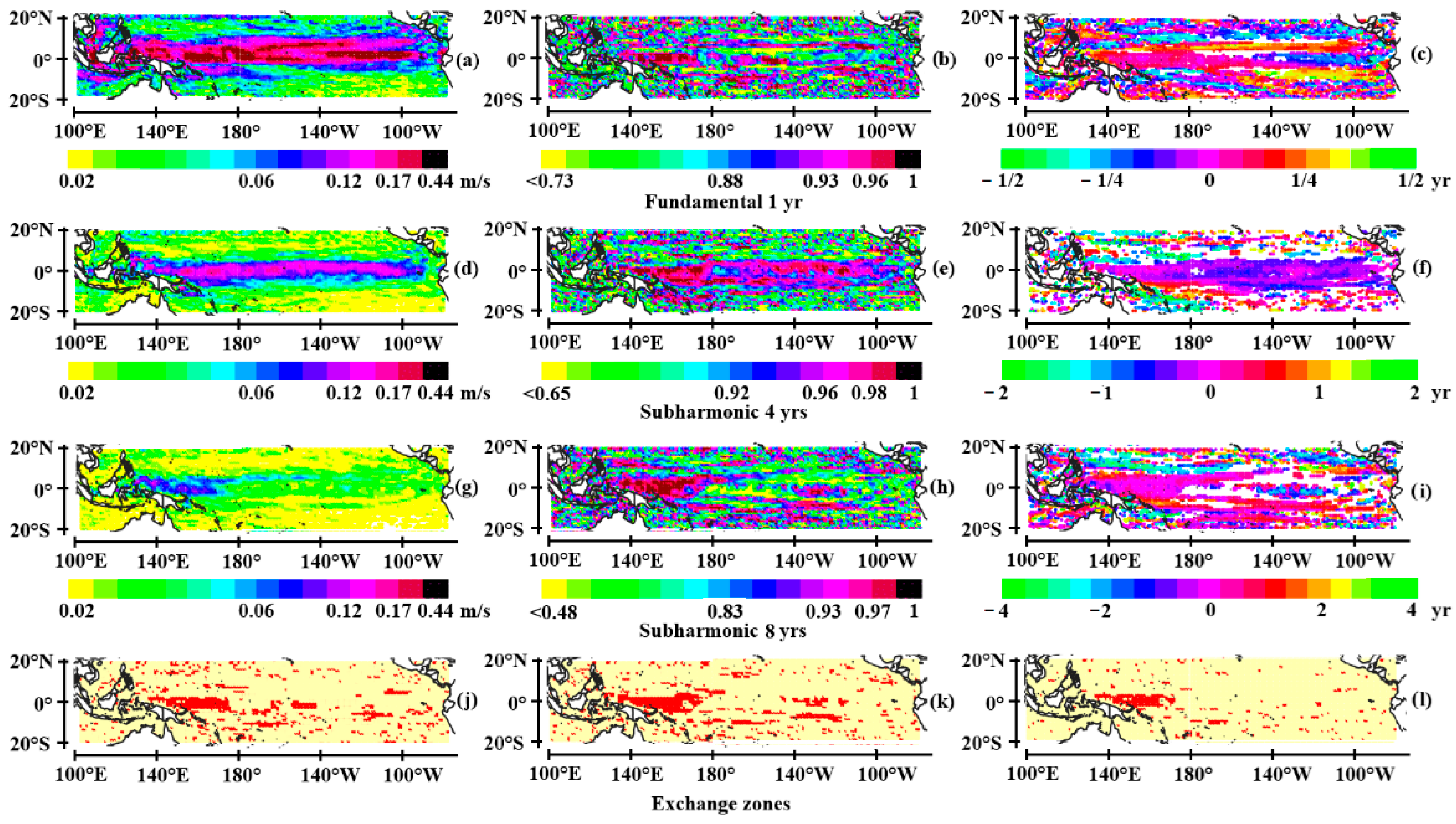
Figure 2.
The same as Figure 1, on 15/12/2006.
Figure 2.
The same as Figure 1, on 15/12/2006.
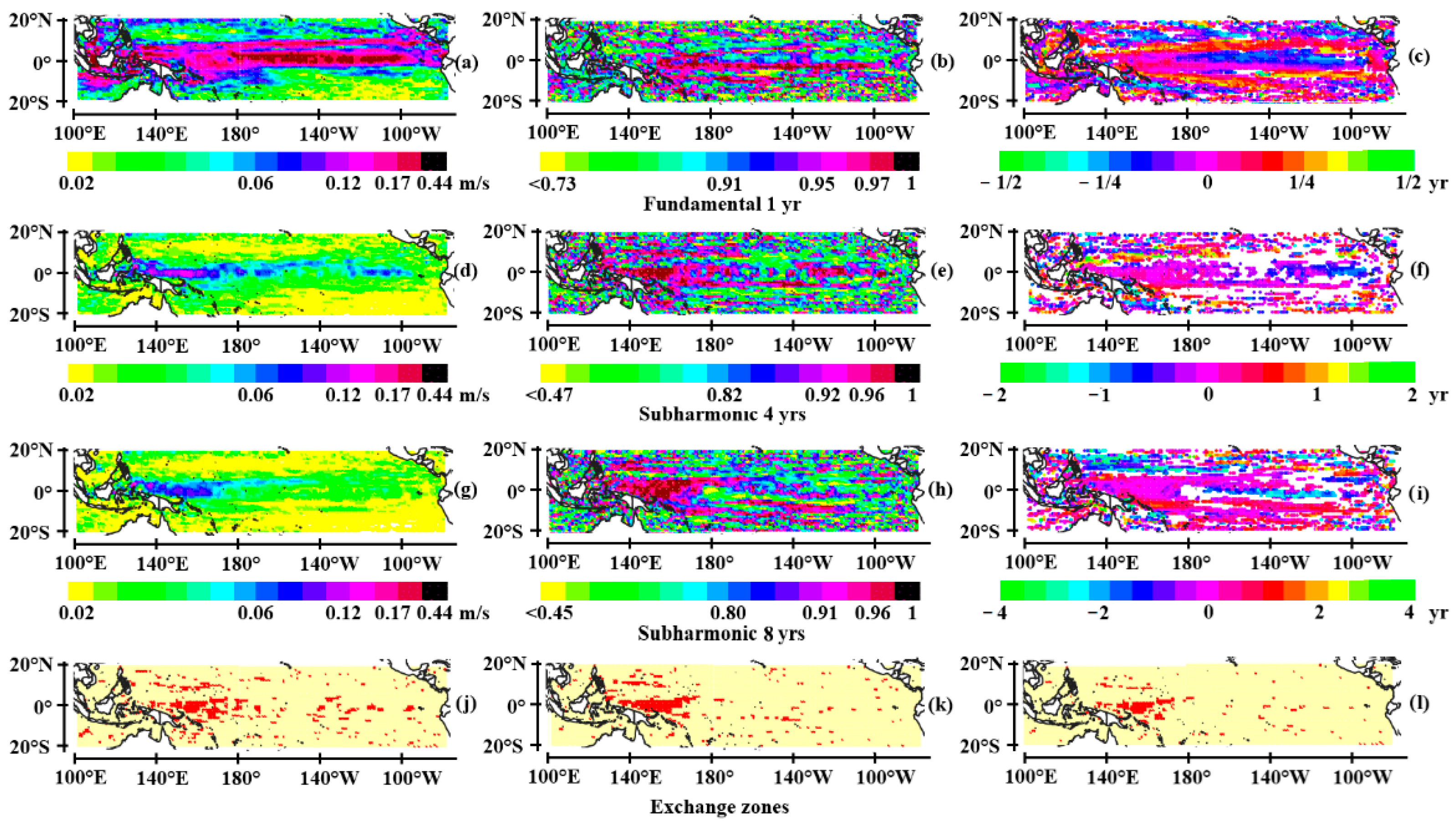
Figure 3.
The time lags (in years) within the four-year cycle. In red, the El Niño–Southern Oscillation (ENSO) event is out of phase with the annual quasi-stationary wave; in green, it is unlagged; in light blue, it is weakly lagged; and in dark blue, it is strongly lagged. Black segment represents the forbidden lag (no event can occur). From [42], Figure 3, with kind permission Copyright 2022 from Journal of Marine Science and Engineering (JMSE).
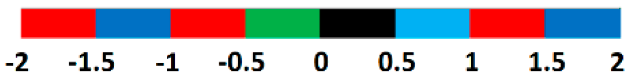
Figure 4.
Amplitude scale-averaged over the 3-6 year range (blue curve) and the 6-12 year range (red curve) of the geostrophic current velocity at 0.5°N, 159.5°E. The bars represent ENSO events (The date of occurrence corresponds to the minima of the Southern Oscillation Index (SOI), i.e. the height to the -SOI value).

Figure 5.
The Tropical Atlantic on 01/01/2005: amplitude (a, d), coherence (b, e) and phase (c, f), scale-averaged in the 0.37–0.75 year range (a, b, c), 0.75-1.5 year range (d, e, f) of the geostrophic current velocity. The temporal reference is the geostrophic current velocity at 0.5°N, 22.5°W (the annual maximum of the eastward geostrophic current velocity is observed in January-February). The phase is represented where the temporal coherence is the most significant. The exchange zone where the coupling of multi-frequency wave systems occurs is represented in red for the subharmonics 0.5 year-1 year (g), which is defined so that the average temporal coherence of the two subharmonics is greater than 0.95.
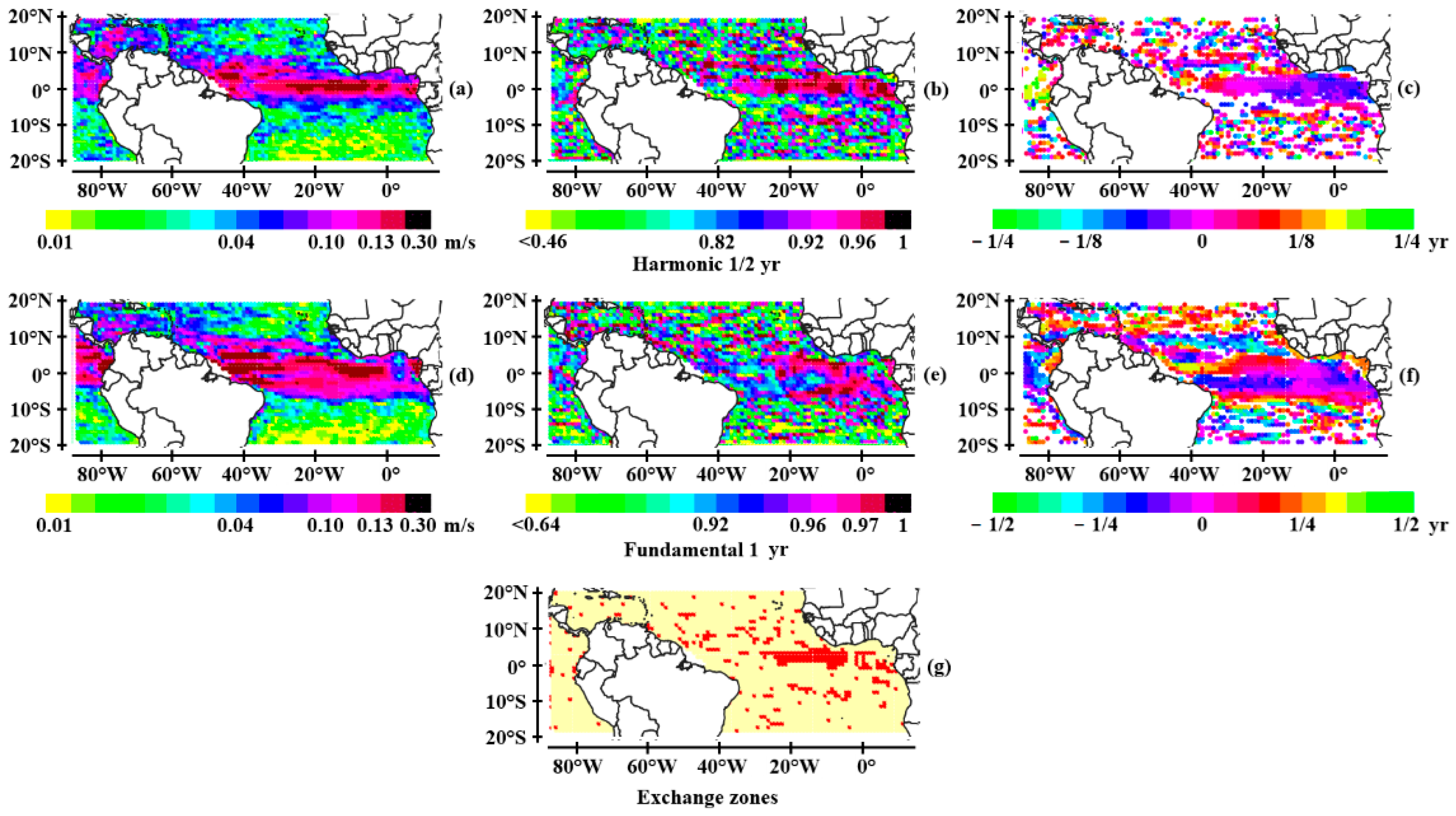
Figure 6.
The Tropical Indian Ocean on 01/01/2005: Amplitude (a, d, g), coherence (b, e, h) and phase (c, f, i), scale-averaged in the 0.37–0.75 year range (a, b, c), 0.75-1.5 year range (d, e, f), and 3-6 year range (g, h, f) of the geostrophic velocity. The temporal reference is the geostrophic current velocity at 0.5°N, 54.5°E (the annual maximum of the eastward geostrophic current velocity is observed in September-October). The phase is represented where the temporal coherence is the most significant. Exchange zones where the coupling of multi-frequency wave systems occurs are represented in red (j, k, l), for the subharmonics 1/2 year-1 year (j), 1 year-4 years (k), and 1/2 year-4 years (l). Exchange zones are defined so that the average temporal coherence of the two subharmonics is greater than 0.95.
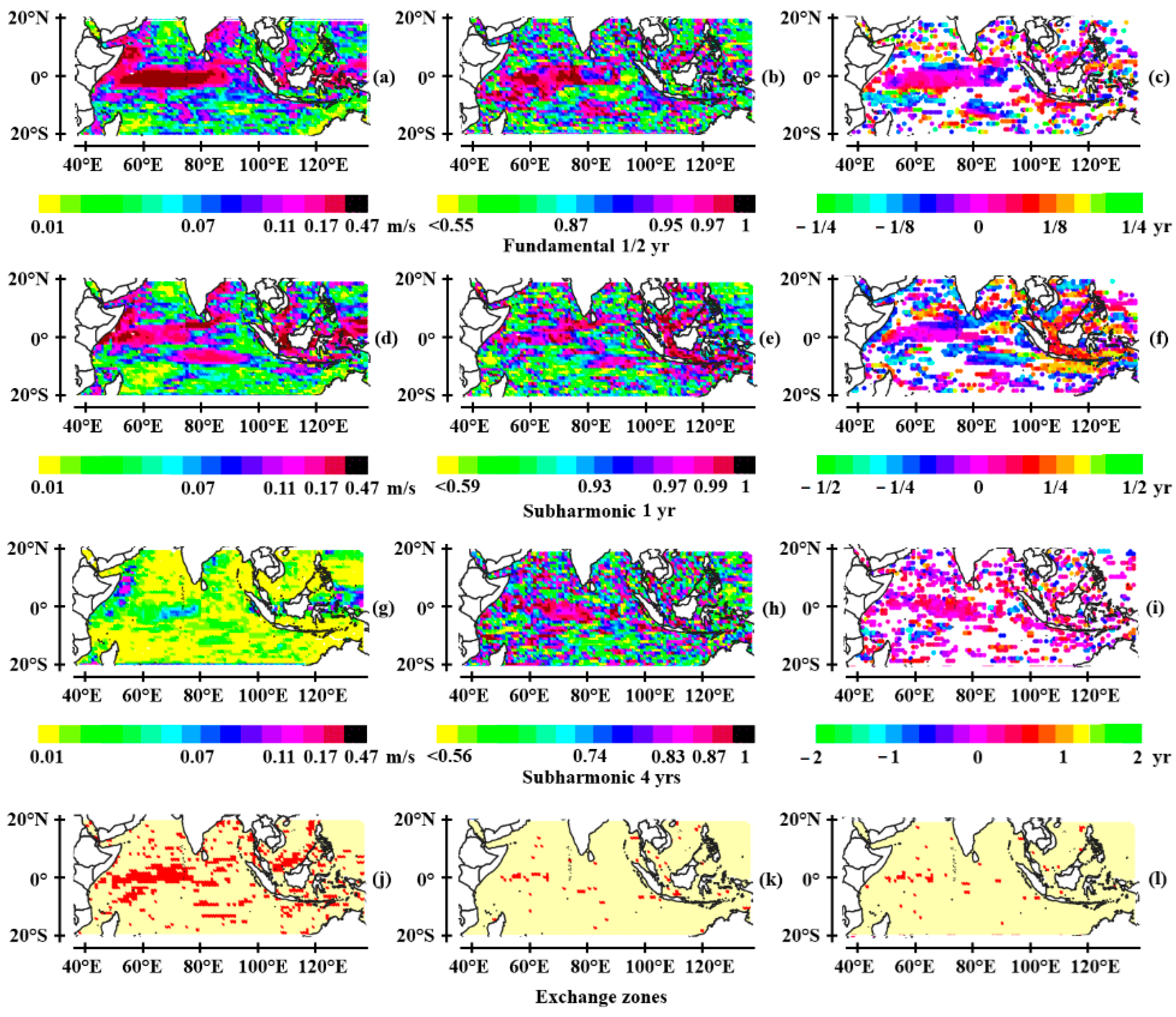
Figure 7.
Wind velocity at 250 mb (facing east) in the Northern Hemisphere on 01/01/2002 in the period ranges 0.75/128 – 1.5/128 year (a, b, c), 0.75/32 – 1.5/32 year (d, e, f), 0.75/16 – 1.5/16 year (g, h, i), 0.75/8 – 1.5/8 year (j, k, l), 0.75-1.5 year (m, n, o), and 1.5-3 years (p, q, r): amplitude in (a, d, g, j, m, p), coherence in (b, e, h, k, n, q) and phase in (c, f, i, l, o, r). The temporal reference used for determining the coherence and the period is the wind velocity at 30°N, 0°E (the annual maximum of the eastward wind velocity is observed in January). The phase is represented where the temporal coherence is the most significant. Exchange zones where the coupling of multi-frequency Rossby waves occurs are represented in red (s, t, u), for the harmonics 1/128 year-1 year (s), 1/32 year-1 year (t), and 1/16 year-1 year (u). Exchange zones are defined so that the average temporal coherence of the two harmonics is greater than 0.95.
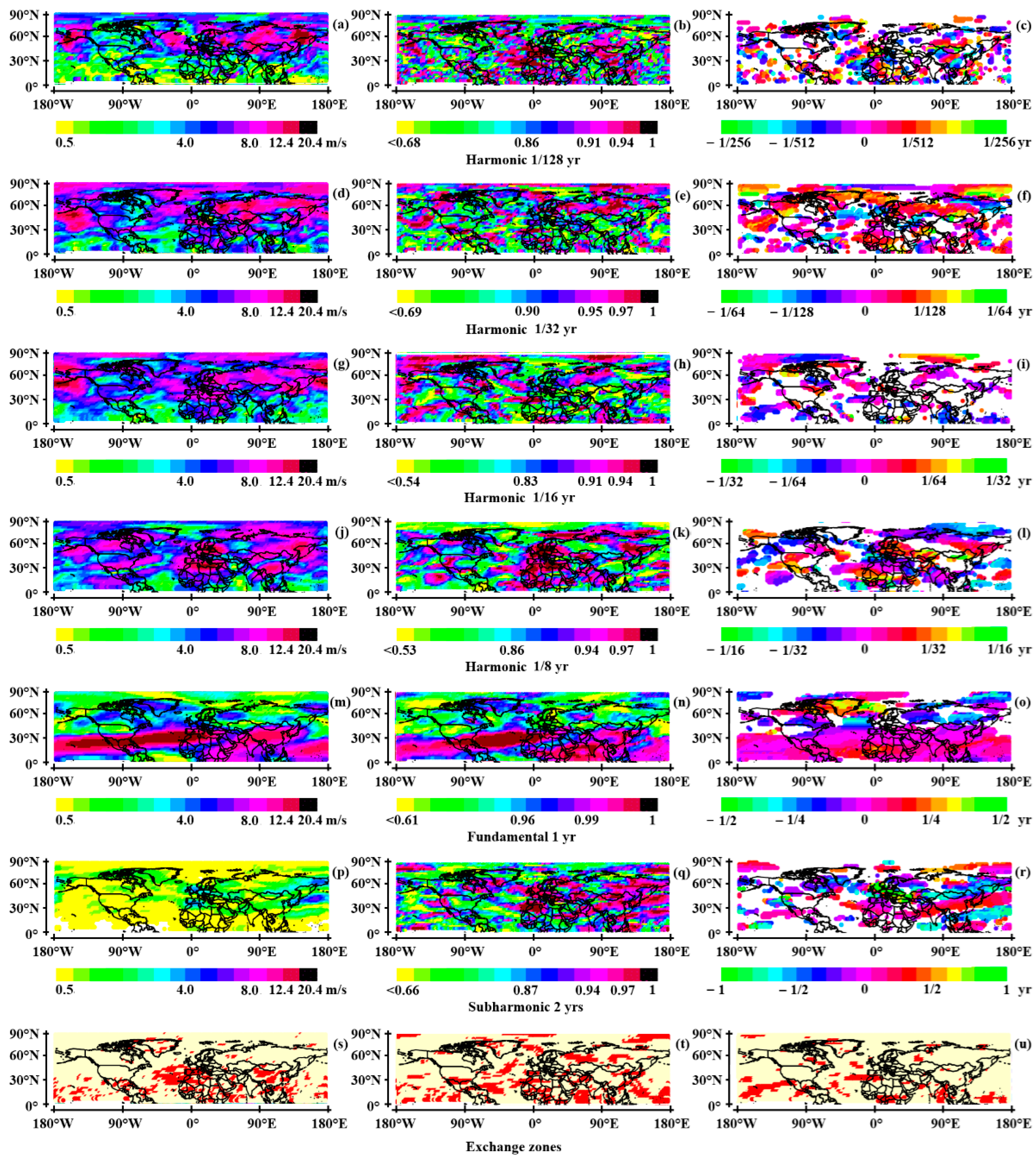
Figure 8.
The cross-section of the Rossby waves at the tropopause of the northern hemisphere vs. latitude.
Figure 8.
The cross-section of the Rossby waves at the tropopause of the northern hemisphere vs. latitude.
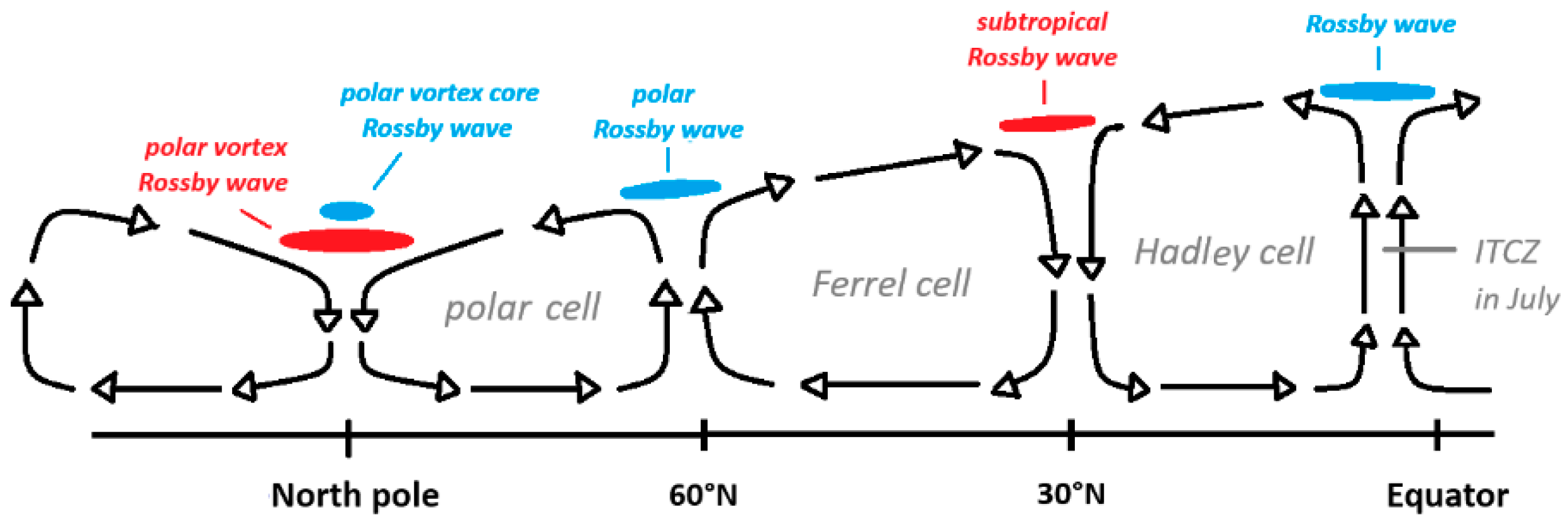
Figure 9.
Wind velocity at 250 mb (facing east) in the Southern Hemisphere on 01/07/2002 in the period ranges 0.75/128 – 1.5/128 year (a, b, c), 0.75/32 – 1.5/32 year (d, e, f), 0.75/16 – 1.5/16 year (g, h, i), 0.75/8 – 1.5/8 year (j, k, l), 0.75-1.5 year (m, n, o), and 1.5-3 years (p, q, r): amplitude in (a, d, g, j, m, p), coherence in (b, e, h, k, n, q) and phase in (c, f, i, l, o, r). The temporal reference used for determining the coherence and the period is the wind velocity at 30°S, 0°E (the annual maximum of the eastward wind velocity is observed in July). The phase is represented where the temporal coherence is the most significant. Exchange zones where the coupling of multi-frequency Rossby waves occurs are represented in red (s, t, u), for the harmonics 1/128 year-1 year (s), 1/32 year-1 year (t), and 1/16 year-1 year (u). Exchange zones are defined so that the average temporal coherence of the two harmonics is greater than 0.95.
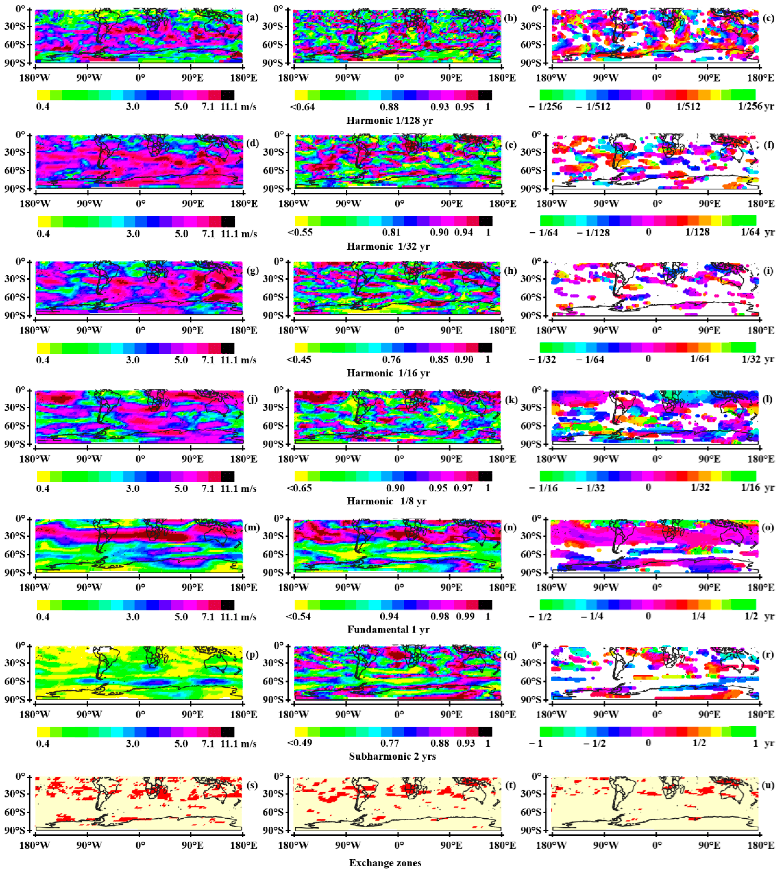
Figure 10.
Geostrophic current velocity in the North Atlantic on 01/01/2005 in the period ranges 0.75/24 – 1.5/24 year (a, b, c) – 1.5/6 year (d, e, f), 0.75/3 – 1.5/3 year (g, h, i), 0.75-1.5 year (j, k, l), and 6-12 years (m, n, 0): amplitude in (a, d, g, j, m), coherence in (b, e, h, k, n) and phase in (c, f, i, l, o). The phase is colored red or blue depending on the apparent traveling direction of the modulated geostrophic current. The temporal reference is the geostrophic current velocity at 38.5°N, 62.5°W (the annual maximum of the eastward geostrophic current velocity is observed in April-July). Exchange zones where the coupling of multi-frequency Rossby waves occurs are represented in red (p, q, r), for the harmonics 1/12 year-1 year (p), 1/6 year-1 year (q), and 1/6 year-1/3 year (r). Exchange zones are defined so that the average temporal coherence of the two harmonics is greater than 0.95.
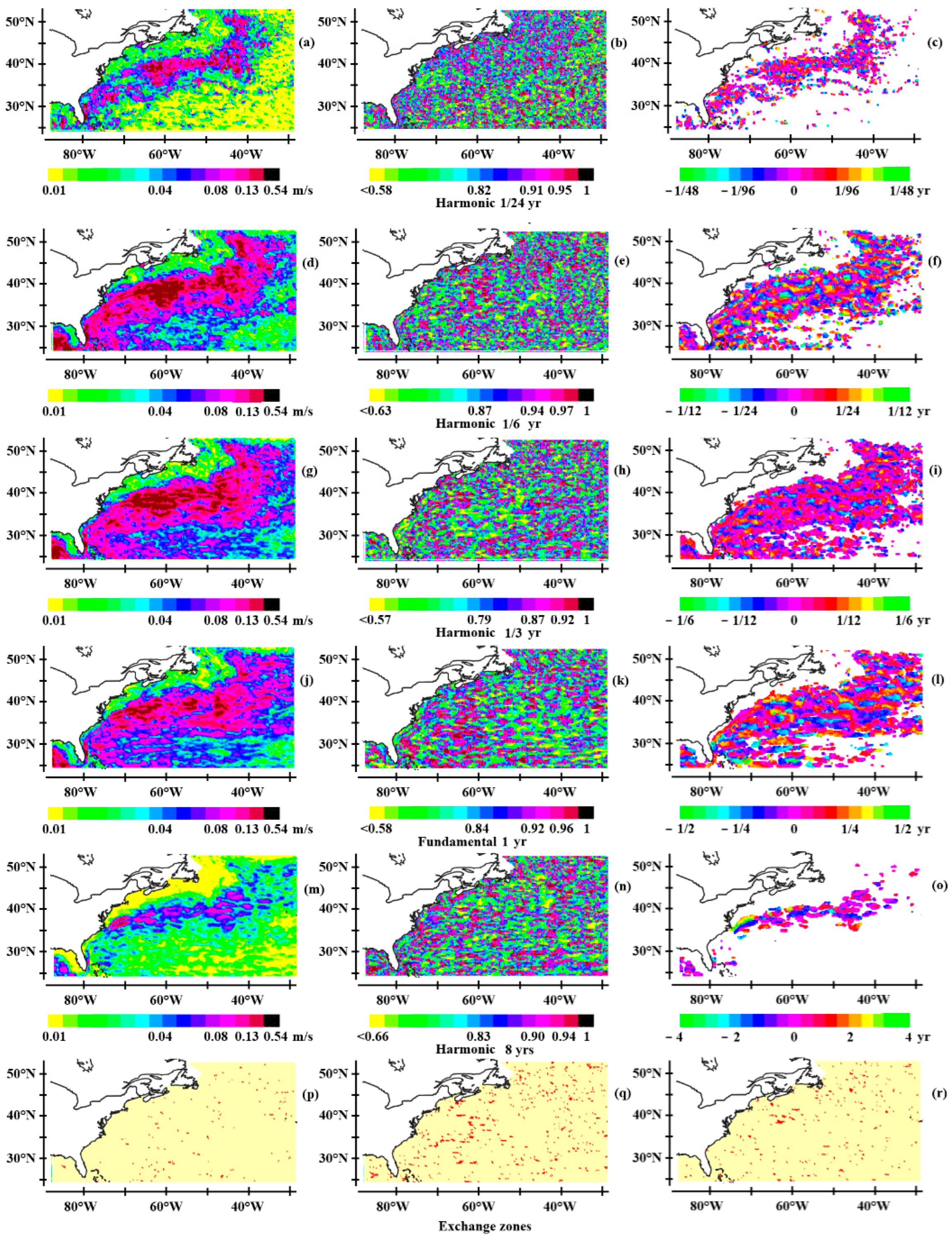
Figure 11.
Maximum of the geostrophic current velocity averaged in the upper quantile (1/500th of the population) vs the period in – (a) the North Atlantic – (b) the South Atlantic – (c) the South Indian Ocean – (d) the North Pacific – (e) the South Pacific. The period is expressed in year on the graphs.
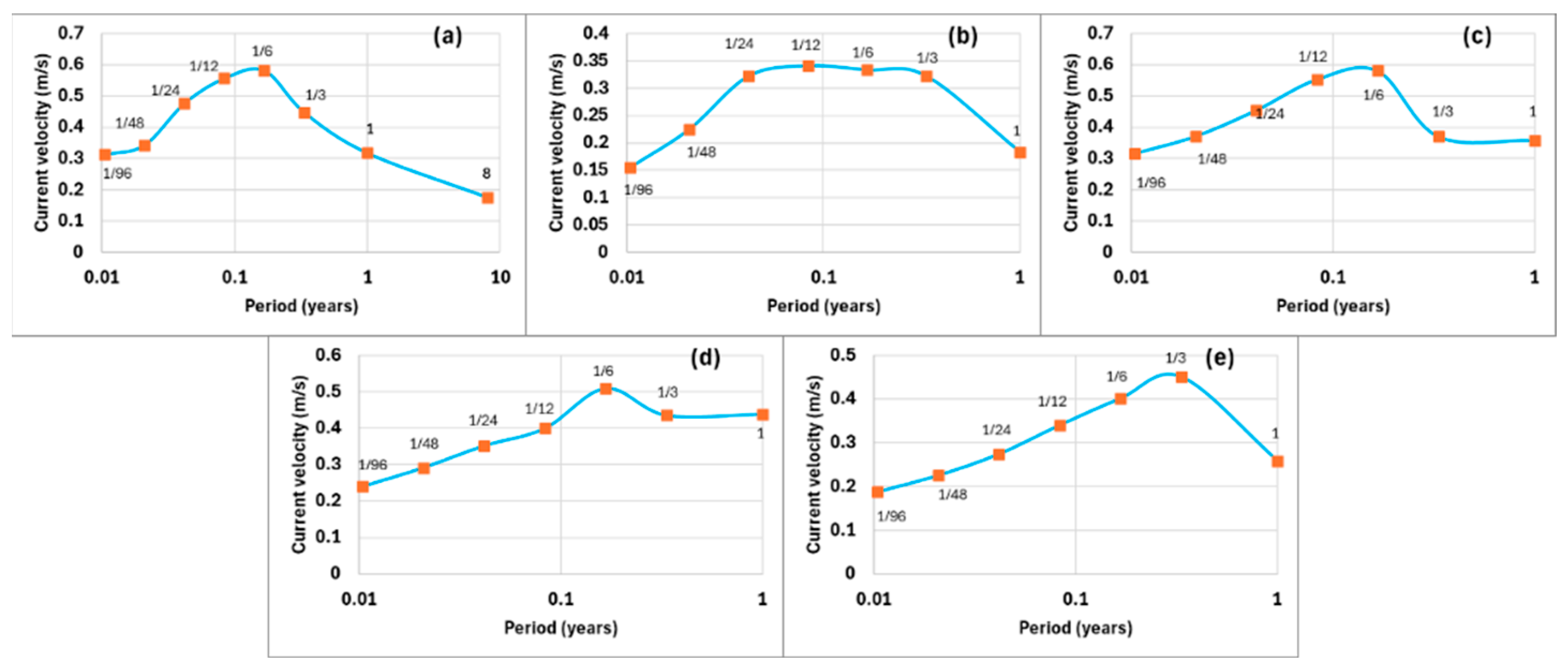
Figure 12.
Geostrophic current velocity in the North Atlantic of the 1/6-yr period harmonic on 01/07/2004 in a, b, c and on 01/01/2005 in d, e, f: amplitude in a, d, coherence in b, e, phase in c, f.
Figure 12.
Geostrophic current velocity in the North Atlantic of the 1/6-yr period harmonic on 01/07/2004 in a, b, c and on 01/01/2005 in d, e, f: amplitude in a, d, coherence in b, e, phase in c, f.
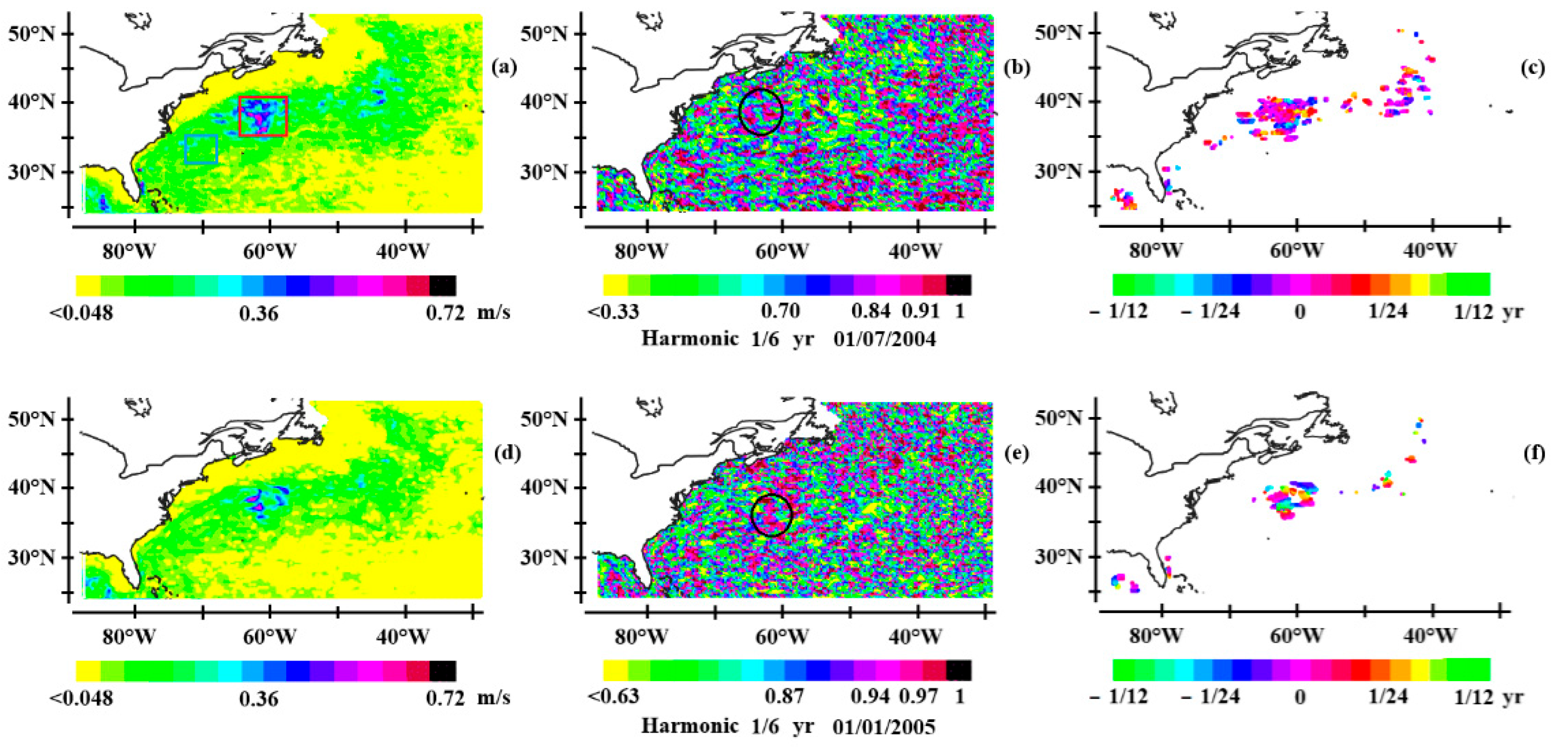
Figure 13.
Geostrophic current velocity in the South Atlantic of the 1/12-yr period harmonic on 01/07/2004 in a, b, c and on 01/01/2005 in d, e, f: amplitude in a, d, coherence in b, e, phase in c, f.
Figure 13.
Geostrophic current velocity in the South Atlantic of the 1/12-yr period harmonic on 01/07/2004 in a, b, c and on 01/01/2005 in d, e, f: amplitude in a, d, coherence in b, e, phase in c, f.
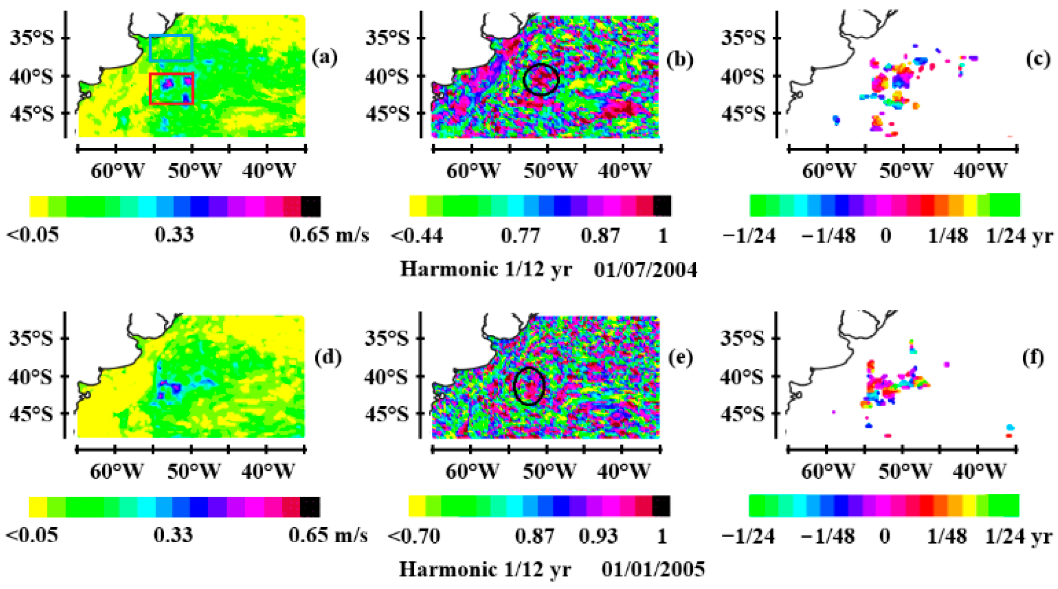
Figure 14.
Geostrophic current velocity in the South Indian Ocean of the 1/12-yr period harmonic on 01/01/2005: amplitude in a, coherence in b, phase in c.
Figure 14.
Geostrophic current velocity in the South Indian Ocean of the 1/12-yr period harmonic on 01/01/2005: amplitude in a, coherence in b, phase in c.
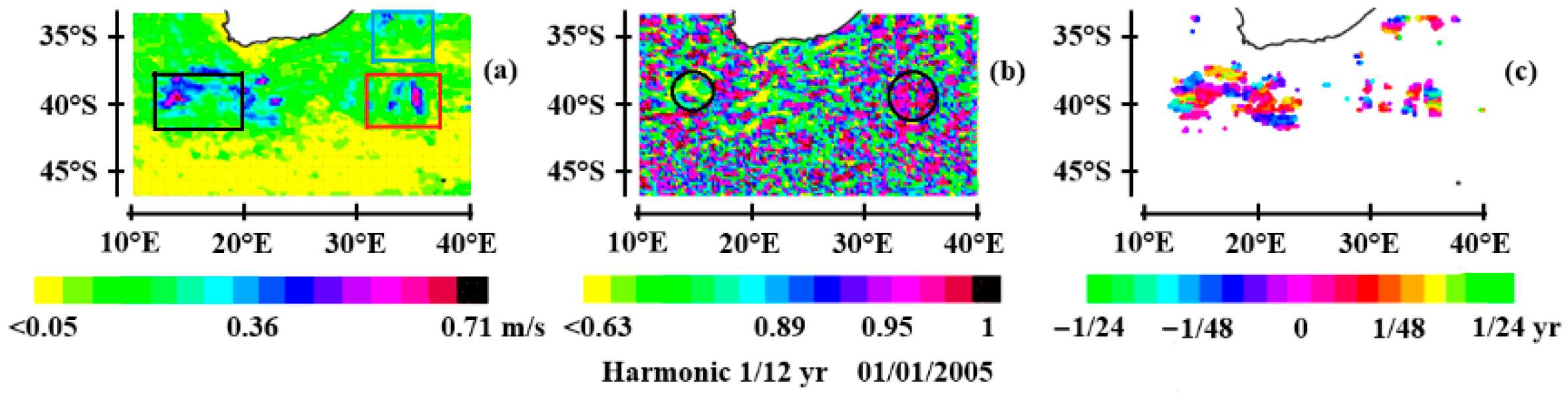
Figure 15.
Geostrophic current velocity in the South Pacific of the 1/3-yr period harmonic on 01/07/2004 in a, b, c and on 01/01/2006 in d, e, f: amplitude in a, d, coherence in b, e, phase in c, f.
Figure 15.
Geostrophic current velocity in the South Pacific of the 1/3-yr period harmonic on 01/07/2004 in a, b, c and on 01/01/2006 in d, e, f: amplitude in a, d, coherence in b, e, phase in c, f.
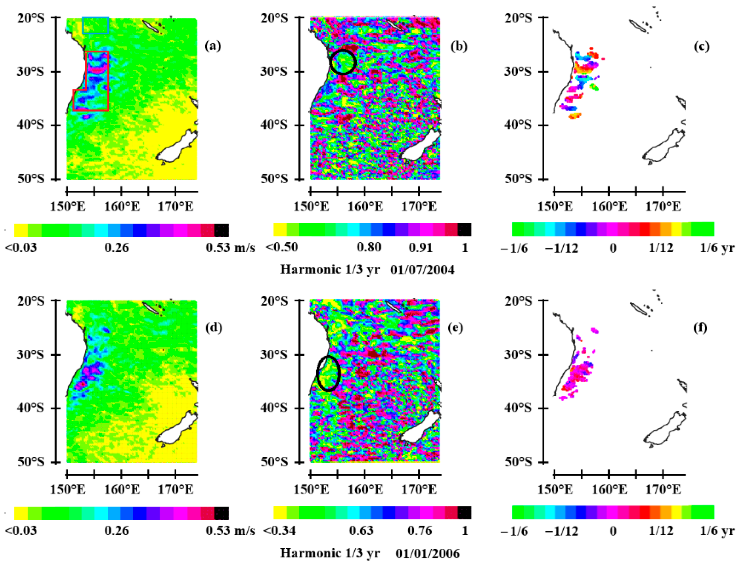
Figure 16.
Geostrophic current velocity in the North Pacific of the 1/6-yr period harmonic on 01/07/2005: amplitude in a, coherence in b, phase in c.
Figure 16.
Geostrophic current velocity in the North Pacific of the 1/6-yr period harmonic on 01/07/2005: amplitude in a, coherence in b, phase in c.
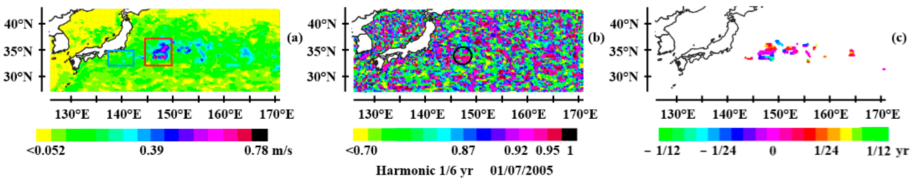
Figure 17.
Annual variations of Sea Surface Temperature (SST) in the regions defined in Figure 12a, Figure 13a, Figure 14a, Figure 15a and Figure 16a. The curves represent the first derivative of third-degree polynomial fits of monthly SST since 1974. Their colors correspond to the colors of the regions.

Figure 18.
Coherence and phase of the Sea Surface Temperature (SST) time-averaged over the period of 1854–2023 (Fourier spectrum), scale-averaged over the period ranges 3–6 years (a,b), 6–12 years (c,d), 12–24 years (e,f), 24–48 years (g,h), and 48–96 years (i,j). The coherence is divided into 16 quantiles. The phase is shown for high values of coherence (8 upper quantiles). Coherence of the Sea Surface Temperature (SST), time-averaged over 1854–2023, scale-averaged over the period range 3–6 years (k), and amplitude of the geostrophic current velocity time-averaged over 1993–2022, scale-averaged over the period range 3–6 years (l). References are the SST at 36◦ S, 36◦ W in (a–k) and the geostrophic current at 36.5◦ S, 50.5◦ W (l).
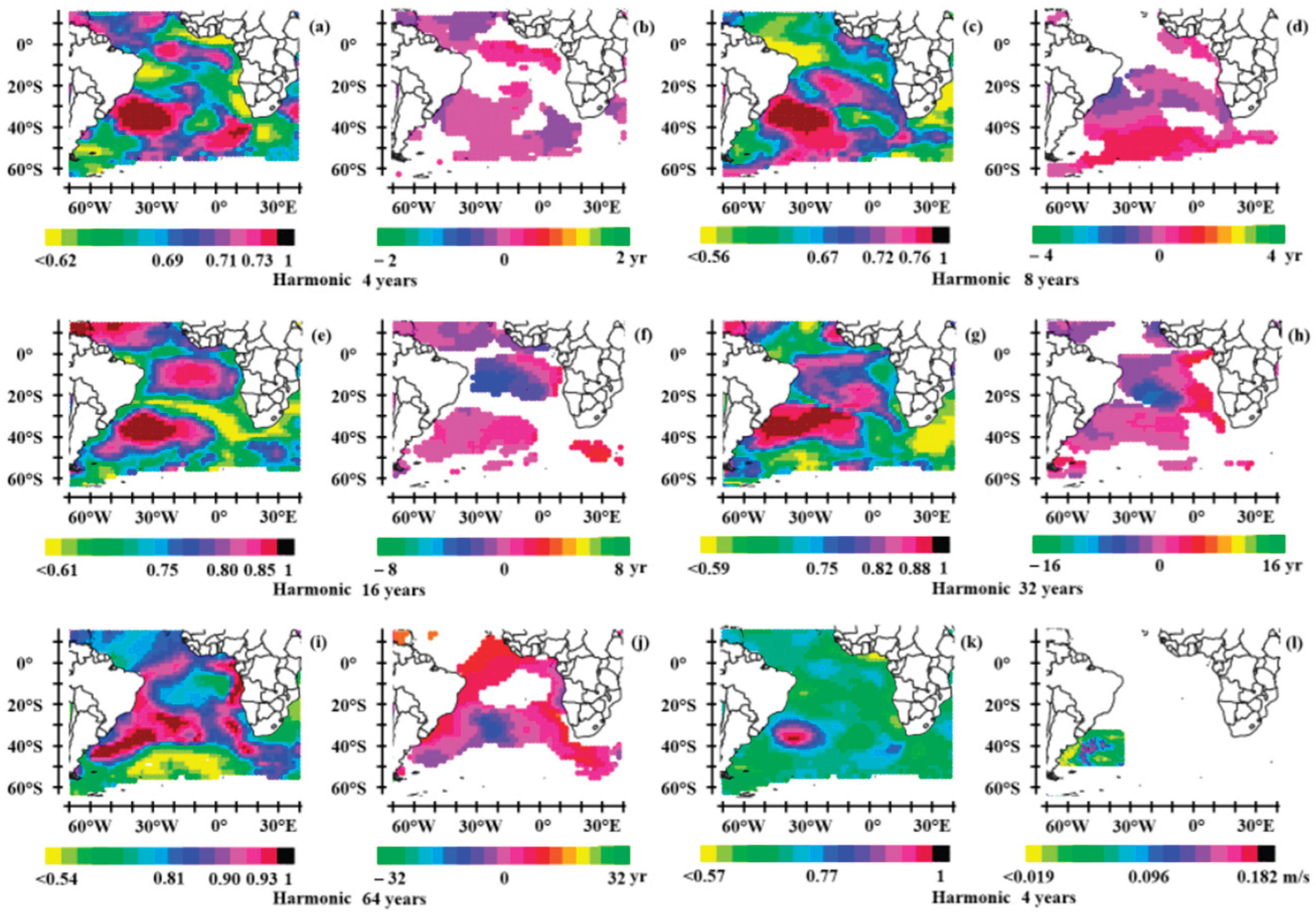
Figure 19.
Exchange zones of subharmonic couples of average periods (1 yr–4 yr) in (a), (4 yr–16 yr) in (b), (4 yr, 64 yr) in (c), and (32 yr, 64 yr) in (d). These zones, which cause resonant forcing to occur in subharmonic modes are defined from the joint coherence of the coupled waves: the areas in red are such that the mean coherence of the coupled waves is higher than 0.85.
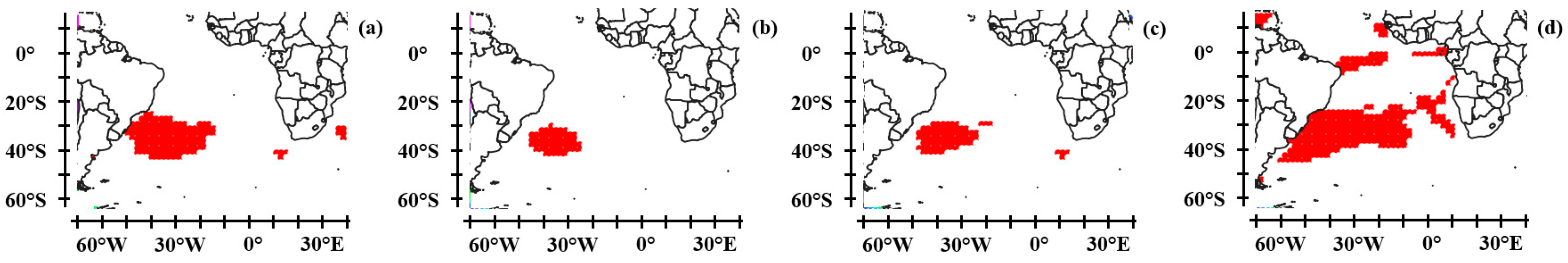
Disclaimer/Publisher’s Note: The statements, opinions and data contained in all publications are solely those of the individual author(s) and contributor(s) and not of MDPI and/or the editor(s). MDPI and/or the editor(s) disclaim responsibility for any injury to people or property resulting from any ideas, methods, instructions or products referred to in the content. |
© 2025 by the authors. Licensee MDPI, Basel, Switzerland. This article is an open access article distributed under the terms and conditions of the Creative Commons Attribution (CC BY) license (http://creativecommons.org/licenses/by/4.0/).
Copyright: This open access article is published under a Creative Commons CC BY 4.0 license, which permit the free download, distribution, and reuse, provided that the author and preprint are cited in any reuse.


