
Submitted:
07 October 2025
Posted:
09 October 2025
You are already at the latest version
Abstract
The NELIPS acronym stands for Nano-Enhanced Laser Induced Plasma Spectroscopy. Within this framework, the temporal variation of the enhanced plasma emission from pure nanomaterials with respect to corresponding bulk materials was monitored as a function of delay time in the range from 1 to 5-11 ms. Six different materials were employed including silver, zinc, aluminum, titanium, iron and silicon . Radiation from pulsed Nd: YAG laser at wavelength 1064 nm was used to induce the bulk and pure nanomaterial plasmas under similar experimental conditions. Plasma emission from both targets was monitored via optical emission spectroscopy technique (OES). The spectral line intensities (signal-to-noise ratio S/N) from the pure nanomaterial plasma turn out to decline in a constant logarithmic manner but at a slower rate than that from the corresponding bulk material plasma. Consequently, the measured average enhanced emission from different nanomaterials features an increase in an exponential manner with delay time. This trend was accounted for by a mathematical elaboration of enhanced emission based on the measured signal-to-noise data. Both plasma parameters (electron density and temperature) evolution during plasma expansion has been illustrated as well.
Keywords:
Enhanced-Emission
; NELIPS
; Temporal variation
; Plasma parameters
1. Introduction
Intense laser radiation from pulsed laser sources above plasma ignition threshold leads to immediate ignition of luminescent plasma at the surface of irradiated target material. Under assumption that, the emitted light from plasma is influenced by plasma parameters [1,2,3], the plasma emission is resolved and analyzed using optical emission spectroscopy (OES) - technique. The laser induced plasma spectroscopy is more concerned with the spectroscopic study of the plasma generated by lasers. This incorporates the state of plasma thermodynamical equilibrium [1], the set of equilibrium distribution relations that can be applied to describe this state [2,3], plasma dynamics [4], spectral line shape analysis [5], including line shift and asymmetry [6], plasma opacity via self-absorption process [7] and the inhomogeneity of plasma produced by focusing laser light on targets [1,2,3,7,9]. In this regard, the enhanced emission from targets made of pure nanomaterials have been reported [8,9,10].
Interestingly, the interaction of pulsed lasers with pure nanomaterials was found to produce very luminescent plasmas than that produced from the pure bulk counterpart of similar stoichiometry under similar experimental condition [8,9,10]. This inherent tendency for plasma enhanced emission has been thoroughly investigated within the framework of Nano-Enhanced laser induced plasma spectroscopy (NELIPS) [10]. This approach is more concerned with the regular practical study and modeling of the observed strong plasma emission when pure nanomaterials irradiated with pulsed lasers [9,10]. Traditional optical emission spectroscopy (OES) technique was employed in conjunction with basic thermodynamics was considered as the recommended theoretical approach [10]. Parametric experimental results on laser and target dependent enhanced emission were empirically modeled and reported in the collective review article [10].
Meanwhile, the experimental measurements were carried out almost at one arbitrary salient transition wavelength [8,9,10]. Moreover, the previously published work in refs [8,9] lacks a reliable theoretical modeling that can describe the temporal variation of enhanced emission. In addition to the suggested problem of sintering of nano particles when compressed in tablet shaped by press.
In this article, six different nanomaterials were employed including Silver, Zinc, Aluminum, Silicon, Iron and Titanium together with their respective bulk counterparts with similar stoichiometry. The detailed of cross-check measurements of the supplied nanoparticle sizes is presented in Appendix C, utilizing the NELIPS-Technique. The amount of enhanced emission is assessed via proper employment of several spectral lines emitted from each type of element utilizing the facilities of the OES-technique. A rigorous theoretical relation describing the measured temporal variation of amount enhanced emission in NELIPS approach was fully elaborated in Appendix A. The measurements of plasma parameters (electron density and temperature) were carried out at each delay time for both types of plasma originated from pure nanomaterial and its bulk counterpart.
2. Experimental Setup and Methodology
This study constitutes only one part of a series of parametric studies of pulsed laser interaction with pure nanomaterials in comparison to its bulk counterpart [8,9,10] supported with theoretical modeling. The experimental setup is described in detail in refs [8,9]. It comprises Nd: YAG laser (type Brilliant B) of pulse duration time of 5 ns working at a wavelength of 1064 nm while the level of laser fluence was kept at constant level of 6.3±0.5 J/cm2. Both targets were positioned at distance of 98 mm from the laser focusing lens (of focal length of 100 mm). The laser spot size was measured using thermal paper (supplied from Quantel®) at the target surface and found as a spot of circular shape with radius 0.73 ± 0.03 mm. The optical emission of the induced plasmas in open air was monitored during fixed camera gate time of 1 μs while the delay time was detuned in the range from 1 to 5 μs and for some nanomaterials (Al, Ti, Ag) the delay time was extended up to 11 μs.
The optical emission spectroscopy (OES) detection system (apparatus) comprises SE200-Echelle type spectrograph equipped with time controlled ICCD-Camera (type Andor, model-iStar-DH734-18F). The light emitted from different plasmas was brought to spectrograph entrance hole using a 25 μm quartz optical fiber with fair optical throughput. The other end of the fiber tip was kept at a fixed distance of 15 ± 1 mm from the laser-plasma axis and caped with replicable special quartz cap to protect the tip of the fiber from the sputtered hot species from plasma. The monitored plasma emission is spatially integrated. The whole operation including laser firing, synchronization, and data acquisition is normally controlled by simple computer - camera interface run by KestrelSpec 3.9® software while all the calculations and analysis were carried using a homemade routines utilizing facilities of the standard MTLALB8®.
Six different types of nanomaterials were employed together with their respective bulk counterparts. Ferrous oxide nanomaterial (Fe3O4) with purity 99 % (MKN-Fe3O4-M20) was supplied in the form of magnetic nano-powder crystals of size diameters of around 20 nm. This has been confirmed using the established NELIPS - Technique [refer to Appendix C] which yields nanoparticles size diameters of (20 ± 1 nm). Likewise, lipophilic titanium oxide (TiO2) was supplied in the form of nano-powder [MKN-TiO2- R020W] with a certified purity of 92 % with nanoparticle diameter size of 20 nm [(20 ± 1) nm [see Appendix C]. Moreover, zinc mono oxide (ZnO) supplied in nanopowder form [MKN-ZnO-030; 1314-13-2] with certified purity of 99.9 %, has particle diameters of (30 nm) within 1% accuracy according to NELIPS - Technique [refer to Appendix C]. A pure silver powder [MKN-Ag-090] of nanoparticles having a diameter of 90 nm has been verified by the supplemented technique to incorporated particles of sizes about 90 ± 2 nm [see Appendix C]. A pure silicon powder of yellow - brown color (purity 99.9 %) of average particle size diameter is 40 nm (MKN-Si-040). The aluminum nanomaterial was supplied in the powder form of average particle size around 40 nm (MKN-Al-040). The supplied nano-powder is molded as a plane target using the popular double face sticker which adsorbs the nano-powder until being saturated. This simple method is adopted to avoid problems that may arise from nanoparticle-sintering during compression into tablet form [8,9]. Both of bulk and nanomaterial targets were fixed on a specially designated homemade xyz-ϕ-holder which allow for irradiation of targets in open air under similar conditions. Data acquisition is the result of accumulated plasma emission over three consecutive laser shots on different target spots to ensure a fresh target condition.
3. Results and Discussion
3.1. Measurement of Plasma Electron Density and Temperature
Accurate measurment of plasmas electron densities is usually carried out utilizing the unique properties of the Hα-line at 656.27 nm [11] which was identified in all emission spectrua. Whithin the framework of NELIPS, the relative electron density is the more likely factor which determine any changes in the values of electron density from the bulk material based plasma to that from the coresspounding nanomaterial based plasma. Figure 1 (A–C) presents an example of the measured normalized spectral line shapes of the Hα-line utilizing emission spectra from Silver, Zinc and Aluminum (bulk-based plasma emission is plotted in black color and nanomaterial-based plasmas is plotted in red color) with measured values of plasma electron densities are depicated in each subfigure. A similar set of 60 - figures were processed at each delay time and for each element presented in both forms (nanomaterial and bulk counterpart) with the numerical results are given in Table A1 in Appendix B.
On the other hand, a reliable measurement of the electron temperature of laser induced plasma is normally carried out via Boltzmann plot method [1,2,3,8,9] provided that certain tight criteria are being met. For plasma in the state of local thermodynamical equilibrium , the spectral lines should be well-resolved, optically thin and originate from the same atomic species with relatively large difference in the upper excited energy [1,2,3,8,9].
In order to construct perfectly straight Boltzmann line, other two corrections should be applied. First, the emission spectral radiance of each of the selected lines at different wavelengths should corrected by the relative spectral sensitivity of the used apparatus including ICCD-Camera and SE200 spectrograph in addition to the used caped optical fiber [8,9]. Second, the spectral radiance of the employed lines should further be corrected against distortions in line shape caused by plasma self-absorption (if exists) [7] and this correction is based on good knowledge of the Stark broadening parameter of each transition line taken into consideration.
Figure 2 (A,B) demonstrates the application of Boltzmann plot method (following the previous procedures) to measure the plasma electron temperatures. The lower dashed stright line was constructed for spectral lines emerged from plasma orginated from the bulk-based plasma while the upper solid line indicates the plasma induced at the suface of nanomaterial. Figure 2 (A) was assigned to Ag (I) spectral lines at wavelengths of 546.54, 520.90, 768.77, 827.35, 338.28 and 328.06 nm (at a delay time of 3 μs), while Figure 2 (B) concerns with Zn (I) spectral lines at the wavelengths of 481.08, 472.20, 468.01, 636.23, 334.55 and 330.27 nm (monitored at a delay time of 5 μs).
A set of other 46 - similar plots were constructed (4 – elements (silver, silicon zinc and aluminum)) at 6 – values of delay times (6 values of delay times with 2- states of matter "Nanomaterial and corresponding bulky material") which resulted in a set of 48 – straight Boltzmann plots. The overall results are presented in the Table A1 (Appendix B).
Close inspection to the overall results in Table A1 (Appendix B) would evidently validate the assumption laid within the framework of NELIPS [8,9,10] namely;and at a fixed delay time.
So far, an example of the temporal variation of electron density (as measured from bulk and nanomaterial targets) with delay time is presented in Figure 3 (A) utilizing the data of Silver element, while the temporal variation of measured electron temperature is shown in Figure 3 (B) utilizing the data of the Zinc element.
A glance to Figure 3 (A,B) indicates a monotonic decrease in both of plasma parameters. A set of 8 - other similar figures are available for other elements which show the same trend of variation of electron density and temperature.
3.2. Measurement of Average Enhancement Over Different Wavelengths
Actually, there are two methods to calculate. The first is via utilizing the Boltzmann plot method which yields precise values of the average enhanced emission [9], but, however, it requires good knowledge of atomic parameters for each employed lines e.g. (transition probability, statistical weight and energy of upper state, Stark broadening parameters [12,13,14,15]). This is in addition to the lengthy procedures of corrections to spectral lines intensities to perfectly align the data points to the straight Boltzmann plot (as can be seen in Figure 2).
The other method is simpler and doesn't require such lengthy procedures. It is based on the direct calculation of the ratio,
Here, is the average amount of spectral lines intensities emitted from the nanomaterial plasma over wavelength interval band and is the corresponding quantity for the bulk counterpart plasma in the same range of wavelengths.
This method is more suitable for certain elements e.g. Iron and Titanium which contains a dense spectral emission (too many emission lines per nm), and therefore we carefully set the range of wavelengths from 250 to 580 nm. This range of wavelengths was chosen to avoid the unwanted spectral emission lines originated from the ambient air elements (Oxygen, Nitrogen, and the Hα-line). However, this method may contain some errors. This error was estimated and found in the range around 16 % and resulted from the unwanted spectral lines from elements other than the element of the target material under study. The results of application of this method to Titanium and Iron are shown in Figure 4 (E–H). A close inspection to these subfigures indicates error from 10- 15%. Moreover, we have found that this method can be applied to other elements which are chractrized by strong and well-resolved spectral lines e.g. Silver, Zinc. Aluminum and Silicon. The avaraging process can be written as for the nanomaterial based plasma and its coresspounding bulk material based plasma with index (n) is the number of lines that will be taken into consideration. Consequently, the avarage enhancement ove the considered spectal lines can be expressed as,
The following set of wavelengths were chosen for different nanomaterials;
- a)
- Silver : Ag I - lines at wavelengths 328.02, 338.2, 520.9, 546.5, 768.7 and 827.3 nm,
- b)
- Zinc: Zn I - lines at wavelength 330.29, 334.55, 468.2, 472.2, 481.01, and 636.38 nm,
- c)
- Aluminum: Al I - lines at wavelengths 308.2, 309.3, 394.8, 396.15 nm
- d)
- Silicon: Si I - lines at wavelengths 288.15, 390.55.
It is worth noting that these spectral lines are not subjected to corrections agianst self-absorption (SA) nor spectral senstivity of the used appartus. Moreover, the calculated avarage spectral radiance and are named wih average signal to ratio (S/N) as shown in the set of sub-figures at Figure 4.
3.3. Modeling of the Temporal Variation of Enhanced Emission NELIPS
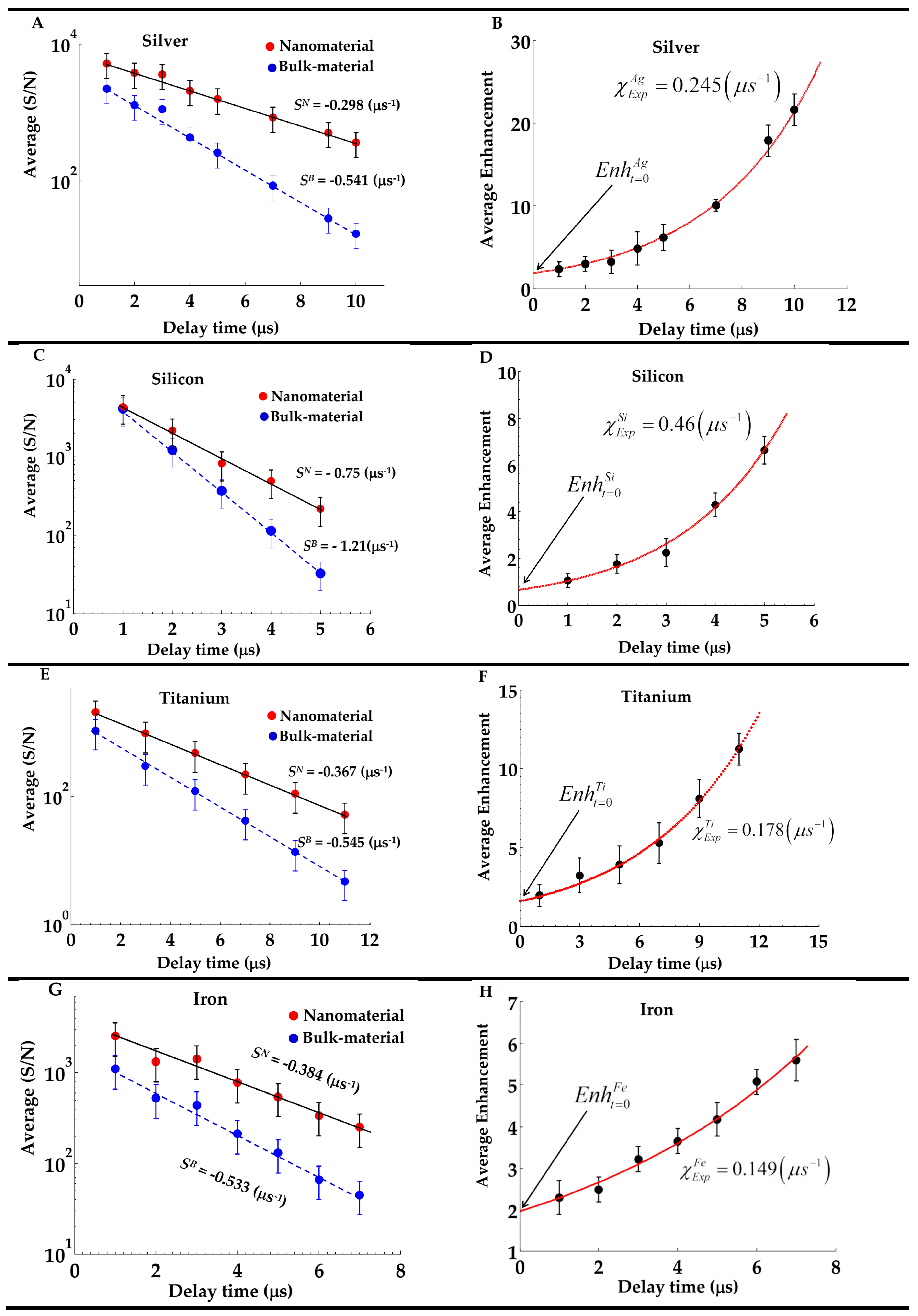
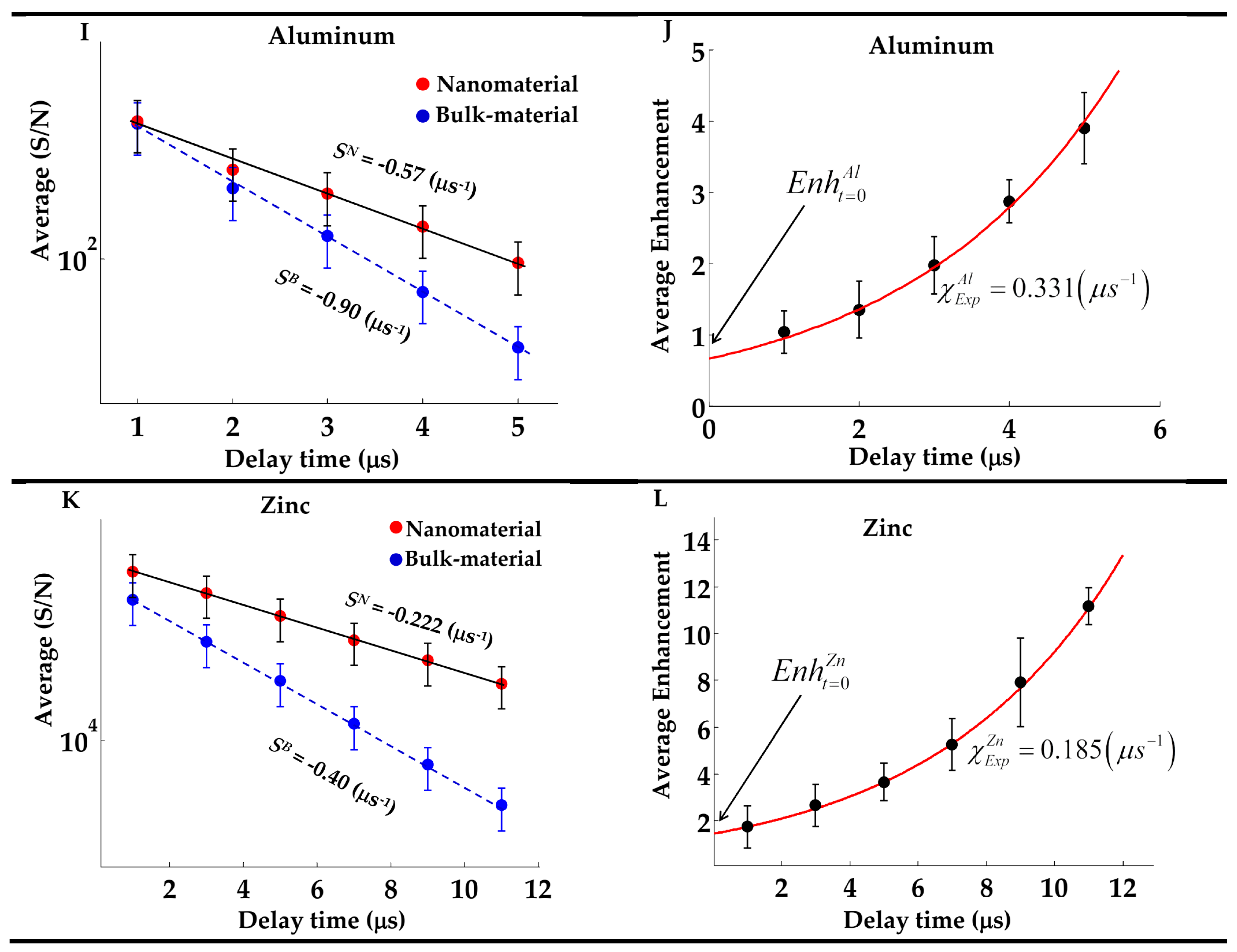
A close inspection of Figure 4 (B,D,F,H,J,L) elicits an exponential growth of the amount with delay time. Hence, one can start from the following simplified relation,
The solution of this simple differential equation can be written as, (detailed derivations in Appendix A),
Where represent the initial enhancement at the zero time delay (τ = 0), and the speed of variation of the exponential function with time, respectively.
Figure 4 (B,D,F,H,J,L) shows the evaluated numerical values of these parameters at the best fitting of expression (4) to measured data points.
Moreover, the detailed derivations (given in Appendix A) show that the exponent fitting parameteris expressed in terms of the difference between the slopes of the straight lines appeared in Figure 4 (A,C,E,G,I,K),
The numerical values of the evaluated slopes at the best fitting are depicted in Figure 4 (A,C,E,G,I,K) which indicates the quality of the suggested modeling. Meanwhile, these slopes and feature the rates of plasma radiative energy loss during plasma expansion process. This would inevitably imply that a nanomaterial plasma luminosity decline at a relatively lower rate than its bulk counterpart as well as it differs from one element to another.
These conclusions in the previous paragraph would encourage us to conduct further and deeper investigations to correlate these rates of radiative energy losses to the basic physical mechanisms responsible of the process of enhanced mission from pure-nanomaterial with different delay times. Now the raised questions are; why this happen when nanomaterials irradiated by pulsed lasers? Further, is this happen if one induces plasma from nanomaterials by different method e.g. using inductively coupled plasma ICP and/ or by arc discharge? Another raised question, is enhanced emission is an inherent property of nanomaterial?
4. Conclusions
Within the framework of NELIPS approach, the temporal variation of the average enhanced plasma emission over different emission wavelengths is explored. Nanomaterials and their bulk-counterparts plasmas including silver, zinc, aluminum, silicon, iron and titanium turn out to nearly share similar plasma electron density and temperatures during plasma expansion. However, the monitored average amount of emission enhancement reveals to exponentially increase with delay time which could be correlated with the recorded slower rate of radiative emission by the plasma generated from the pure nanomaterials. These experimental findings are compatible with mathematically suggested approach.
Author Contributions
Conceptualization, A.E.S.; methodology, A.E.S.; software, A.E.S.; validation, A.E.S. and A.A.; formal analysis, A.E.S.; investigation, A.E.S.; data curation, A.E.S.; writing—original draft preparation, A.E.S.; writing—review and editing, A.E.S. and A.A.; visualization, A.E.S. and A.A.; supervision, A.A. All authors have read and agreed to the published version of this manuscript.
Funding
This research received no external funding.
Data Availability Statement
The data presented in this study concerning NELIPS are available upon a reasonable request from the corresponding author.
Acknowledgments
The authors would like to express their deepest gratitude to the Quantum Beam Sci.-MDPI-Publishing-House. Special acknowledgement should be addressed to the MTC (Department of Physics and mathematics) for the supply of the different nanomaterials used in this study via MOU (SAMAA000-37-2022XT).
Appendix A
Mathematical derivation of the temporal variation of enhanced emission
One can start from the basic definition of enhanced emission,
The rate of change of enhanced emission with time can be expressed as,
This can be simply expanded as,
On rearranging, we obtain,
After rearrangement we get,
This derivative can be rewritten as,
Implicitly, this implies that one should use the logarithm of the spectral line intensities.
Integrating both sides of (A6) yields the final solution as,( which is similar to expression(4))
The exponent factor is appeared in equation (A6),
Appendix B
Results of measurement of plasma parameters in a limited range of delay time (1-5 μs)

Table A1.
The measured plasma parameters; nanomaterial-based target (marked in red color) and bulk-based target (marked in blue color).
Table A1.
The measured plasma parameters; nanomaterial-based target (marked in red color) and bulk-based target (marked in blue color).
| Measured electron density (× 1017 cm-3) with associated error margins | ||||||||||||||||||
|---|---|---|---|---|---|---|---|---|---|---|---|---|---|---|---|---|---|---|
| Delay | 1 μs | 2 μs | 3 μs | 4 μs | 5 μs | |||||||||||||
| Element | Nano | Bulk | Nano | Bulk | Nano | Bulk | Nano | Bulk | Nano | Bulk | ||||||||
| Ag | 4.29 ± 0.1 | 4.2 ± 0.08 | 1.8 ± 0.12 | 1.79 ± 0.10 | 0.89 ±0 .04 | 0.89 ± 0.03 | 0.55 ± 0.15 | 0.55 ± 0.13 | 0.23 ± 0.04 | 0.23 ± 0.05 | ||||||||
| Zn | 4.4 ± 0.66 | 4.7 ± 0.70 | 2.5 ± 0.90 | 2.4 ± 0.80 | 1.2 ± 0.40 | 1.4 ± 0.50 | 0.7 ± 0.26 | 0.70 ± 0.24 | 0.64 ± 0.08 | 0.54 ± 0.07 | ||||||||
| Si | 4.37 ± 0.8 | 4.1 ± 0.50 | 1.5 ± 0.09 | 1.45 ± 0.09 | 0.78 ± 0.07 | 0.77 ± 0.08 | 0.42 ± 0.08 | 0.45 ± 0.07 | 0.37 ± 0.02 | 0.34 ± 0.05 | ||||||||
| Al | 4.6 ± 0.66 | 4.7 ± 0.70 | 2.2 ± 0.90 | 2.3 ± 0.80 | 1.2 ± 0.40 | 1.1 ± 0.50 | 0.69 ± 0.26 | 0.68 ± 0.24 | 0.54 ± 0.08 | 0.54 ± 0.07 | ||||||||
| Fe | 4.42 ± 0.8 | 4.8 ± 0.50 | 1.47 ± 0.09 | 1.46 ± 0.09 | 0.83 ± 0.07 | 0.77 ± 0.08 | 0.42 ± 0.08 | 0.43 ± 0.07 | 0.35 ± 0.02 | 0.33 ± 0.05 | ||||||||
| Ti | 3.4 ± 0.7 | 3.4 ± 0.03 | 1.8 ± 0.08 | 1.7 ± 0.03 | 0.99 ±0 .05 | 0.91 ± 0.04 | 0.72 ±0 .07 | 0.69 ± 0.02 | 0.52 ± 0.04 | 0.54±0.03 | ||||||||
| Measured electron temperatures (eV) with associated error margins | ||||||||||||||||||
| Delay | 1 μs | 2 μs | 3 μs | 4 μs | 5 μs | |||||||||||||
| Element | Nano | Bulk | Nano | Bulk | Nano | Bulk | Nano | Bulk | Nano | Bulk | ||||||||
| Ag | 1.12 ± 0.1 | 1.06 ± 0.09 | 0.89 ± 0.08 | 0.89 ± 0.06 | 0.72 ± 0.05 | 0.72 ± 0.07 | 0.63 ± 0.07 | 0.60 ± 0.02 | 0.54± 0.04 | 0.55 ± 0.06 | ||||||||
| Zn | 1.25 ± 0.24 | 1.2 ± 0.21 | 0.88 ± 0.14 | 0.89 ± 0.11 | 0.72 ± 0.09 | 0.71± 0.08 | 0.61 ± 0.07 | 0.60 ± 0.05 | 0.50 ± 0.05 | 0.55 ± 0.06 | ||||||||
| Al | 1.1 ± 0.1 | 1.02 ± 0.09 | 0.89 ± 0.08 | 0.89 ± 0.06 | 0.72 ± 0.05 | 0.72 ± 0.07 | 0.63 ± 0.07 | 0.60 ± 0.02 | 0.53± 0.04 | 0.55 ± 0.06 | ||||||||
| Si | 1.05 ± 0.24 | 1.2 ± 0.21 | 0.88 ± 0.14 | 0.89 ± 0.11 | 0.72 ± 0.09 | 0.71± 0.08 | 0.61 ± 0.07 | 0.60 ± 0.05 | 0.50 ± 0.05 | 0.51 ± 0.06 | ||||||||
Appendix C
Application of NELIPS in the measurement of nanoparticle size diameters
This proposed method is based on the direct measurement of the thresholds fluence of laser-plasma ignition for both of nanomaterial and the corresponding bulky counterpart [16].
The following procedures are typically adopted:
- Using the standard NELIPS experimental set up.
- Measure the laser spot size area at the target position in the units of cm2, and measure laser energy per laser shot (in units Joule), then determine the laser fluence in the units of (J / cm2)
- Start with irradiating bulk material and record the plasma emission spectrum.
- Decrease the laser fluence by nearly equal steps (via introducing neutral density filters in the laser beam path) and repeat the previous step until no appreciable optical signal is recorded.
- Plot the relation between laser fluence and the spectral intensity (Signal-To-Noise) ratio of one of the strongest spectral lines e.g. emission from zinc, the wavelength of 480 nm is suitable.
- Under typical experimental conditions, one should repeat the previous procedures for the corresponding nanomaterial.
- Measure the plasma ignition thresholds of both bulk and nanomaterial as shown in Figure B1 at the point of intersection of the backward extrapolation with the horizontal axis. One must notice that .
- With the help of the available standard data tables, find the values of the following thermal quantities of the bulk material in SI units as given in Table A1, are the coefficient of thermal conductivity, density, isochoric heat capacity, respectively.
- With basic knowledge of the laser pulse duration time , one can calculate the thermal diffusion or conduction length of the bulk material using expression.
- Adopting one of the important outcomes of the recently established principle of the NELIPS approach, i.e. If one can measure the laser induced plasma ignition threshold fluence of a bulk material and for the corresponding nano material , the following expression can hold about the relation of the diameter of the nanoparticles with thermal conduction length [16];
In the present experiment, four different nanomaterials of different diameters were supplied (Iron, Titanium, Zinc and Silver) with certified diameters as previously given at the experimental set up. We will demonstrate this procedure for the two materials (titanium and iron).
The thermal quantities of the different bulk materials are given in Table A2. We have used the laser radiation from Nd: YAG working at the fundamental wavelength of 1064 nm with typical pulse duration time Hence, as mentioned at step # 9, one can calculate the thermal conduction lengths of the two bulk materials in the units of (nm), with the results as given in Table A1.
Table A2.
Thermal constants of the used bulk materials.
| Material | ||||
|---|---|---|---|---|
| Titanium | 22 | 4500 | 523 | 216 |
| Iron | 80 | 7870 | 444 | 338 |
| Silver | 429 | 10500 | 237 | 928 |
| Zinc | 111 | 7133 | 383 | 450 |
Figure A1.
Variation of (S/N) ratio with laser fluence (measurement of plasma ignition threshold.
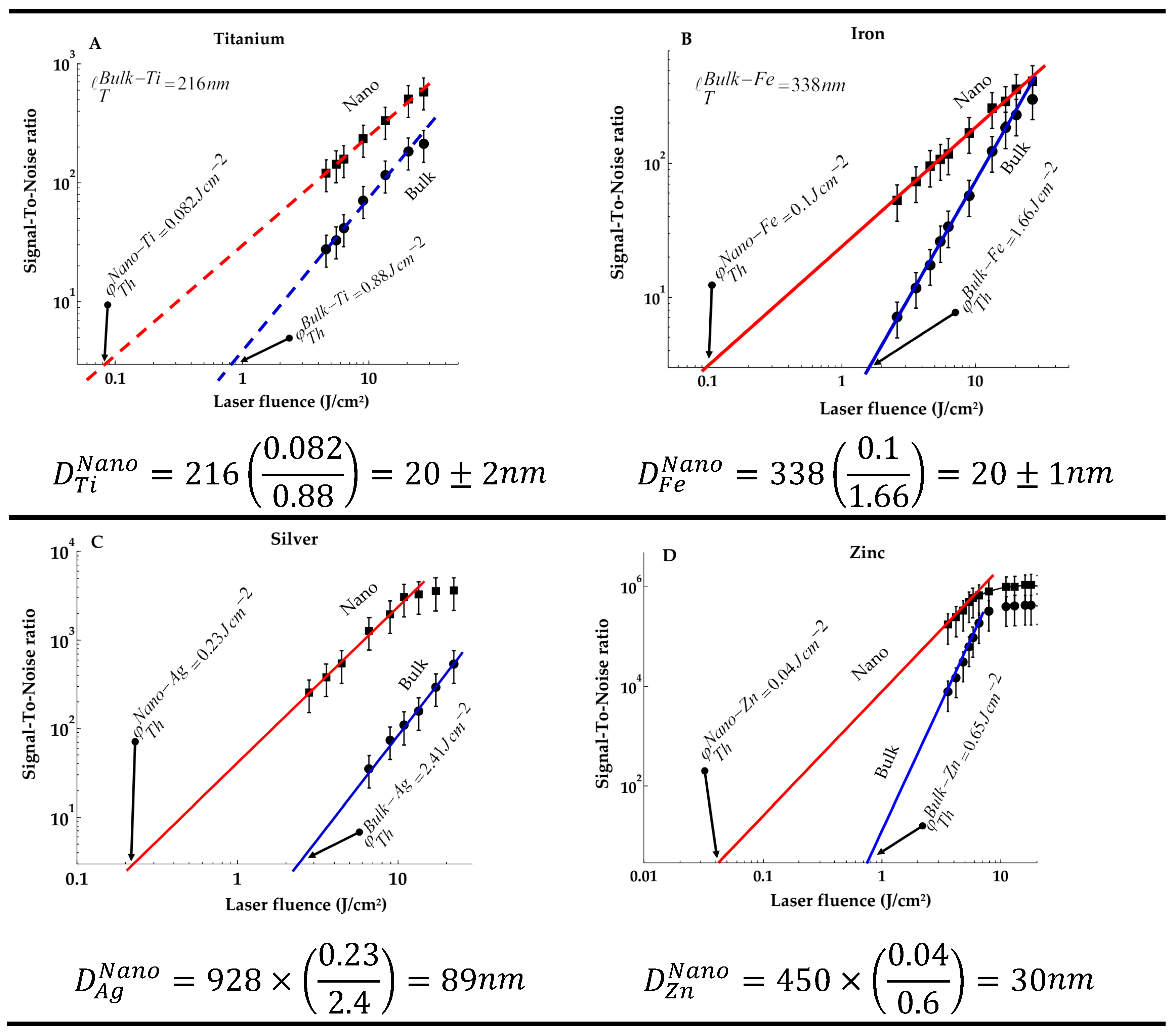
A demonstration of the method of measurement of plasma ignition threshold fluence is presented in Figure A1 (A-D), with numerical results as depicted in each of the subfigures, showing the measured the values of plasma ignition thresholds , together with the estimated diameters of the nanoparticles. It is obvious that the estimated values of the nanomaterial particle diameters adopting NELIPS - approach [10] nearly match those supplied in data sheets.
References
- Cremers, D.A.; Leon, J.R. Handbook of Laser-Induced Breakdown Spectroscopy, 1st ed.; Wiley: Hoboken, NJ, USA, 2013.
- Fujimoto, T. Plasma Spectroscopy. In Plasma Polarization Spectroscopy; Fujimoto, T., Iwamae, A., Eds.; Springer: Berlin/Heidelberg, Germany, 2008; Volume 44, pp. 29–49. [CrossRef]
- Kunze, H.-J. Introduction to Plasma Spectroscopy; Springer Series on Atomic, Optical, and Plasma Physics; Springer: Berlin/Heidelberg, Germany, 2009; Volume 56.
- Tsurutani, B.T.; Zank, G.P.; Sterken, V.J.; Shibata, K.; Nagai, T.; Mannucci, A.J.; Malaspina, D.M.; Lakhina, G.S.; Kanekal, S.G.; Hosokawa, K.; et al. Space Plasma Physics: A Review. IEEE Trans. Plasma Sci. 2023, 51, 1595–1655. [CrossRef]
- Gomez, T.A.; Nagayama, T.; Cho, P.B.; Kilcrease, D.P.; Fontes, C.J.; Zammit, M.C. Introduction to Spectral Line Shape Theory. J. Phys. B: At. Mol. Opt. Phys. 2022, 55, 034002. [CrossRef]
- Sorge, S.; Günter, S. Simulation of Shifted and Asymmetric Hydrogen Line Profiles. The European Physical Journal D 2000, 12, 369–375. [CrossRef]
- Sherbini, A.M.E.; Sherbini, A.E.E.; Parigger, C.G.; Sherbini, T.M.E. Nano-Particle Enhancement of Diagnosis with Laser-Induced Plasma Spectroscopy. J. Phys.: Conf. Ser. 2019, 1253, 012002. [CrossRef]
- Sherbini, A.M.E.; Sherbini, A.E.E.; Parigger, C.G.; Sherbini, T.M.E. Nano-Particle Enhancement of Diagnosis with Laser-Induced Plasma Spectroscopy. J. Phys.: Conf. Ser. 2019, 1253, 012002. [CrossRef]
- EL Sherbini, A.M.; Aboulfotouh, A.; Rashid, F.F.; Allam, S.H.; Dakrouri, A.E.; EL Sherbini, T.M. Observed Enhancement in LIBS Signals from Nano vs. Bulk ZnO Targets: Comparative Study of Plasma Parameters. World J. Nano Sci. Eng. 2012, 2, 181–188. [CrossRef].
- Sherbini, A.E.; Aboulfotouh, A.; Sherbini, T.E. On the Similarity and Differences Between Nano -Enhanced Laser-Induced Breakdown Spectroscopy and Nano-Enhanced Laser-Induced Plasma Spectroscopy in Laser-Induced Nanomaterials Plasma. QuBS 2024, 9, 1. [CrossRef]
- El Sherbini, A.M.; Hegazy, H.; El Sherbini, Th.M. Measurement of Electron Density Utilizing the Hα-Line from Laser Produced Plasma in Air. Spectrochimica Acta Part B: Atomic Spectroscopy 2006, 61, 532–539. [CrossRef]
- Kramida, A.; Ralchenko, Y. NIST Atomic Spectra Database, NIST Standard Reference Database 78 1999.
- Dimitrijević, M.S.; Sahal-Bréchot, S. Stark Broadening of AgI Spectral Lines. Atomic Data and Nuclear Data Tables 2003, 85, 269–290. [CrossRef]
- Dimitrijevic, M.S.; Sahal−Bréchot, S. Stark Broadening Parameter Tables for Neutral Zinc Spectral Lines. Serb Astron J 1999, 21–33. [CrossRef]
- Djurović, S.; Blagojević, B.; Konjević, N. Experimental and Semiclassical Stark Widths and Shifts for Spectral Lines of Neutral and Ionized Atoms (A Critical Review of Experimental and Semiclassical Data for the Period 2008 Through 2020). Journal of Physical and Chemical Reference Data 2023, 52, 031503. [CrossRef]
- El Sherbini, A.M.; Parigger, C.G. Nano-Material Size Dependent Laser-Plasma Thresholds. Spectrochim. Acta Part B At. Spectrosc. 2016, 124, 79–81. [CrossRef]
Figure 1.
Spectral line shapes of the Hα-line. (A) Silver, (B) Aluminum, (C) Zinc.
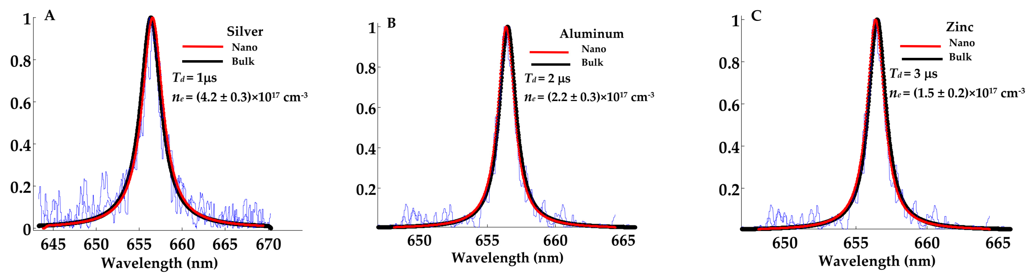
Figure 2.
Boltzmann plots used in the measurment of plasma temperature. (A) Silver at delay time 3 μs, (B) Zinc at delay time 5 μs.
Figure 2.
Boltzmann plots used in the measurment of plasma temperature. (A) Silver at delay time 3 μs, (B) Zinc at delay time 5 μs.
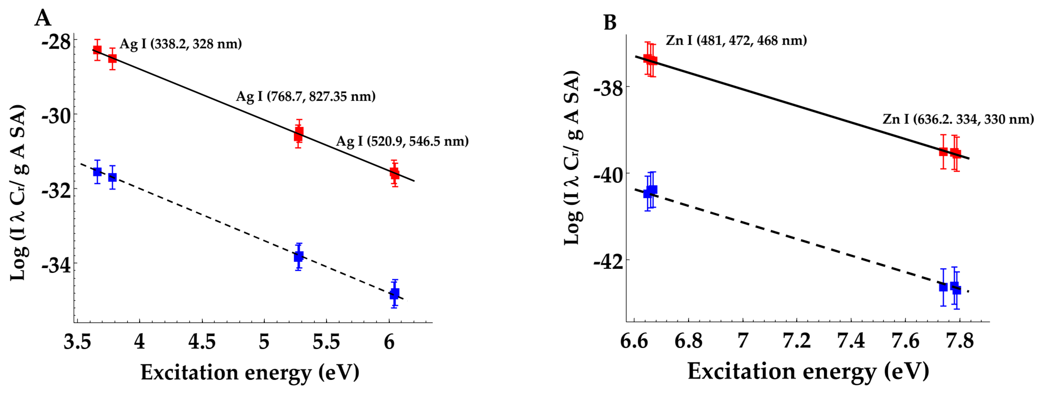
Figure 3.
Example of the temporal variation of plasma parameters (A) electron density (plotted on a logarithmic scale), (B) electron temperature (plotted on a linear scale).
Figure 3.
Example of the temporal variation of plasma parameters (A) electron density (plotted on a logarithmic scale), (B) electron temperature (plotted on a linear scale).
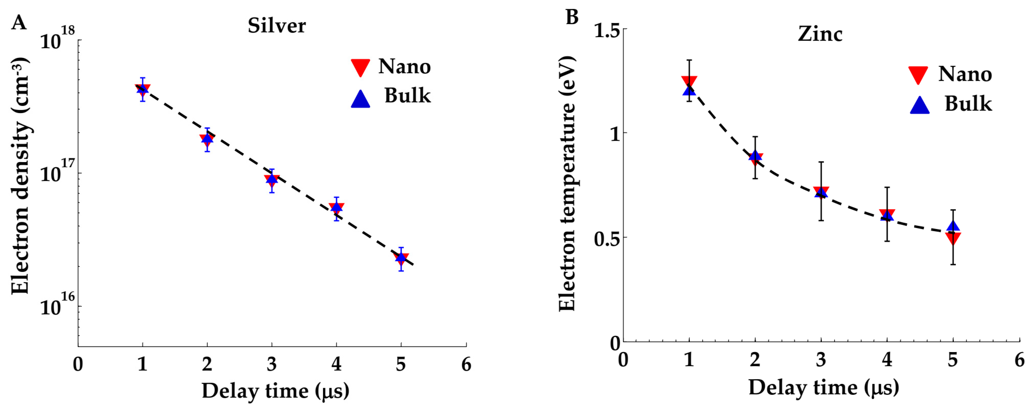
Figure 4.
(A, C, E, G, I, K) Temporal variation of signal-to-noise (S/N). (B, D, F, H, J, L) Temporal variation of enhanced emission, together with the evaluated fitting paramters
Figure 4.
(A, C, E, G, I, K) Temporal variation of signal-to-noise (S/N). (B, D, F, H, J, L) Temporal variation of enhanced emission, together with the evaluated fitting paramters
Disclaimer/Publisher’s Note: The statements, opinions and data contained in all publications are solely those of the individual author(s) and contributor(s) and not of MDPI and/or the editor(s). MDPI and/or the editor(s) disclaim responsibility for any injury to people or property resulting from any ideas, methods, instructions or products referred to in the content. |
© 2025 by the authors. Licensee MDPI, Basel, Switzerland. This article is an open access article distributed under the terms and conditions of the Creative Commons Attribution (CC BY) license (http://creativecommons.org/licenses/by/4.0/).
Copyright: This open access article is published under a Creative Commons CC BY 4.0 license, which permit the free download, distribution, and reuse, provided that the author and preprint are cited in any reuse.


