Submitted:
15 July 2025
Posted:
17 July 2025
You are already at the latest version
Abstract
To address controlled flight into terrain (CFIT) accidents, the Automatic Ground Collision Avoidance System (Auto-GCAS) was developed and implemented. This paper focuses on the trajectory prediction module within the Auto-GCAS. Aiming to overcome the limitations of traditional trajectory prediction algorithms, such as insufficient prediction accuracy and inadequate capability to capture features of nonlinear complex motion trajectories, a trajectory prediction method based on CPO-optimized CNN-LSTM-Attention is proposed. The Crested Porcupine Optimization (CPO) algorithm is employed to optimize the parameters of the CNN-LSTM-Attention network, primarily to determine the optimal learning rate and the optimal number of hidden nodes. Both qualitative and quantitative experimental approaches were adopted, using function simulations to model the complex motion trajectories of fighter aircraft. Comparative experiments were conducted to evaluate the prediction performance of four models: LSTM, CNN-LSTM, CNN-LSTM-Attention, and CPO-CNN-LSTM-Attention. The experimental results demonstrate that the CPO-CLA model exhibits significant advantages in model convergence speed and trajectory prediction accuracy, with notable improvements over the traditional LSTM model in terms of RMSE, MAE, and MAPE metrics.
Keywords:
track prediction
; Crested Porcupine optimizer
; multi-head attention mechanism
; long and short term neural networks
; convolutional neural networks
1. Introduction
Controlled Flight Into Terrain (CFIT) is a serious aviation accident that threatens flight safety [1]. Pilot disorientation and misjudgment of vertical position are the primary causes of such accidents. From 2006 to 2016, CFIT accidents accounted for 35% of all incidents involving the U.S. military’s F/A-18 fighters, resulting in 50% of the total losses and a pilot fatality rate of 73% [2]. As early as the 1980s, the U.S. Air Force began developing an automated response system capable of taking control when pilots lose the ability to operate the aircraft and quickly returning control to the pilot once the collision risk is mitigated [3]. After more than 30 years of research and development, the Automatic Ground Collision Avoidance System (Auto-GCAS) was born and has been progressively implemented across multiple fighter aircraft, including the F-16, F-22, and F-35A [4].
The Automatic Ground Collision Avoidance System adopts a modular design, with its algorithm consisting of four modules: trajectory prediction algorithm, terrain scanning algorithm, collision assessment program, and flight control coupling. The algorithm architecture is shown in Figure 1.
This paper focuses on studying the trajectory prediction algorithm within the Automatic Ground Collision Avoidance System, aiming to accurately capture the motion characteristics of aircraft trajectories, improve prediction accuracy and real-time performance, and lay a solid foundation for the effective application of the system in the future.
Aircraft trajectory prediction is generally categorized into three approaches: state estimation-based methods, flight dynamics model-based methods, and machine learning-based methods.
State estimation-based methods typically describe the aircraft's motion state through mathematical models and perform real-time corrections using observational data. Common techniques include the Kalman Filter (KF) algorithm, particle filter algorithm, Hidden Markov Model (HMM), and their various improved versions [5]. Tang Chenyu et al. [6] leveraged the Kalman filter’s ability to efficiently filter linear noise and predict states, proposing a flight trajectory prediction method based on the Kalman filter, which effectively improved prediction accuracy and reduced computational costs. To address the stability issues of existing trajectory prediction methods, Chen Mingqiang et al. [7] proposed a flight trajectory prediction model based on the Unscented Kalman Filter, enhancing the accuracy and stability of the Extended Kalman Filter algorithm. I. Lymperopoulos et al. [8] tackled the limitations of traditional filtering algorithms in handling high-dimensional nonlinear state predictions for multiple aircraft, proposing a novel particle filter algorithm that integrates air and ground radar data to predict the states of multiple aircraft in non-level flight conditions.
Flight dynamics model-based methods typically involve constructing physical or dynamic models of the aircraft and combining flight data for trajectory prediction. Wang Chao et al. [9] proposed a basic flight model that constructs a model based on multi-stage flight characteristics and achieves 4D trajectory prediction by fitting trajectory feature points. Du Zhuoming et al. [10] proposed an aircraft trajectory prediction method that considers thrust intent and environmental factors based on thrust setting information, reducing the absolute error of the prediction model by 52% compared to traditional methods. X. Zhang et al. [11] adopted a hybrid system recursive approach to study the two distinct phases of flight state transition and continuous flight, obtaining 4D flight trajectories under models for state switching and continuous variation. Suplisson, A. W. from the U.S. Air Force Academy [12] proposed an optimal control method for ground collision avoidance systems in military heavy aircraft, applying control signals to the aircraft’s flight dynamics model using optimal path and control techniques to derive the flight trajectory under control inputs.
Machine learning-based methods typically learn the patterns of aircraft trajectories from historical data to build nonlinear mapping models for predicting future positions, including deep learning methods such as Long Short-Term Memory (LSTM) networks, Convolutional Neural Networks (CNNs), and Transformers. Payeur et al. [13] proposed a method using Artificial Neural Networks (ANNs) to predict robotic trajectories, forecasting future positions by inputting six adjacent coordinates of a moving target. Following Ronald Williams and David Zipser’s introduction of real-time recurrent learning for Recurrent Neural Networks (RNNs) [14], researchers began exploring the feasibility of using RNNs for trajectory prediction. Results showed that RNNs perform well for time-series data like trajectory prediction; however, long sequences and large parameters can lead to gradient explosion or vanishing issues, rendering the network incapable of prediction. To address this, Long Short-Term Memory (LSTM) networks [15] were proposed, incorporating memory cells and gating mechanisms to effectively preserve and update long-term dependencies, excelling in handling long-sequence data. B. Kim et al. [16] used LSTM networks to learn vehicle trajectory data, leveraging their excellent time-series feature capture capabilities to efficiently predict future vehicle trajectories. Z. Zhang et al. [17] optimized the thresholds and initial weights of LSTM networks using an ant colony optimization algorithm, avoiding local optima and effectively improving prediction accuracy and convergence speed. Dai Lican et al. [18] combined KF and LSTM models, using LSTM to learn target motion states and Kalman filtering to dynamically correct state estimates, enhancing the accuracy and effectiveness of flight trajectory prediction. Wang Kun et al. [19] addressed the limitations of traditional trajectory prediction methods by combining attention mechanisms, CNNs, and LSTM, significantly reducing the average error of the prediction model compared to traditional approaches.
In the aforementioned flight trajectory prediction models, methods based on state estimation and flight dynamics models each have their advantages. However, state estimation methods rely on high-precision observation data and have limited capability in handling nonlinear problems, while flight dynamics model-based methods suffer from high computational complexity and insufficient real-time performance. The flight trajectory of a fighter aircraft, beyond the straight flight, turning, climbing, and descending motion states during the route phase, primarily involves complex trajectories during maneuvering. Compared to traditional state estimation and flight dynamics models, deep learning-based methods offer greater advantages. These methods can effectively learn the motion patterns in complex trajectories from time series data, enabling fast and accurate predictions. Therefore, this study on trajectory prediction models is based on a combination of swarm intelligence algorithms and multi-model deep learning methods to ensure robust feature extraction for nonlinear complex motion trajectories and high prediction accuracy.
2. Trajectory Prediction Model Construction
2.1. Crested Porcupine Optimizer (CPO)
The Crested Porcupine Optimizer (CPO) is a novel metaheuristic algorithm proposed by Mohamed Abdel-Basset and colleagues [20] in 2023, designed to precisely address optimization problems involving large-scale data. It draws inspiration from the defensive behaviors of the crested porcupine. When faced with a threat, the crested porcupine employs four distinct self-defense strategies: visual, auditory, olfactory, and physical attack. In CPO, these behaviors are mapped to the process of solving optimization problems, with visual and auditory defense mechanisms serving as exploration strategies, and olfactory and physical attack mechanisms functioning as exploitation strategies. Additionally, a novel strategy called the "Cyclic Population Reduction Technique" is integrated into CPO, mimicking the porcupine’s behavior of activating defenses only when directly threatened. This innovation enables the algorithm to accelerate convergence while maintaining population diversity. The computational steps are as follows.
First, set the parameters , , , , , and ,randomly initialize the population. When , evaluate the fitness of candidate solutions to determine the best solution. Update the defense factor using Equation (1).
Use mathematical model formula (2) to update population size, implementing the cyclic population reduction technique:
Where:
:Population size,
:Convergence speed factor,
: A predefined constant used to balance local exploitation (the third defense mechanism) and global exploration (the fourth defense mechanism),
:A variable that determines the number of iterations,
:Maximum number of function evaluations,
:Modulo operator,
:Minimum number of individuals in the newly generated population.
Therefore, the population size cannot be less than .
When , update and  , and generate two random numbers and ; if , enter the exploration phase and generate two random numbers and ; if , activate the first defense mechanism, formula (3); otherwise, activate the second defense mechanism, formula (4). If , enter the exploitation phase and generate a random number ; if , activate the third defense mechanism, formula (5); otherwise, activate the fourth defense mechanism, formula (6). Iterate over to obtain the global optimal fitness value until .
, and generate two random numbers and ; if , enter the exploration phase and generate two random numbers and ; if , activate the first defense mechanism, formula (3); otherwise, activate the second defense mechanism, formula (4). If , enter the exploitation phase and generate a random number ; if , activate the third defense mechanism, formula (5); otherwise, activate the fourth defense mechanism, formula (6). Iterate over to obtain the global optimal fitness value until .Where:
:The current best solution, serving as the representative of the optimal solution in the Porcupine Algorithm,
:The vector generated between the current best solution and the best solution randomly selected from the population, representing the predator's position at the t-th iteration,
: A binary vector with values in the range of [0, 1],
:Scent diffusion factor,
:A parameter used to control the search direction,
: Represents a random number in the range [0, 1],
: Represents the position of the i-th individual at the t-th iteration, also indicating the predator located at that position,
:The average force acting on the best solution of the i-th predator,
: A random number in the range [0, 1].
2.2. A Trajectory Prediction Model Based on CPO Optimization of CNN-LSTM-Attention
2.2.1. Convolutional Neural Networks (CNN)
Convolutional Neural Networks (CNNs) are widely used feedforward neural networks [21], primarily composed of convolutional layers, pooling layers, and fully connected layers. Their core concept involves using convolutional operations to process data in Euclidean space, offering significant advantages in time-series prediction [22].
This paper adopts a one-dimensional Convolutional Neural Network (1D CNN), which includes convolutional kernels to capture short-term sequence pattern features and share parameters, as shown in Figure 2.
2.2.2. LSTM Network
The Long Short-Term Memory (LSTM) network is a variant of Recurrent Neural Networks (RNNs), overcoming issues like gradient vanishing and explosion, making it highly effective for multi-variable problems. The LSTM architecture includes three gating units: forget gate, input gate, and output gate. State transitions at each time step depend not only on the previous state but also on the combined influence of these gates [23].
Where:
, , :States of the input, forget, and output gates,
:Candidate cell state,
: Current cell state,
:Current hidden state,
:Input sequence value at the current time step,
, , , : Weight matrices for the gates,
: Bias vectors,
:Sigmoid activation function,
: Hyperbolic tangent activation function.
2.2.3. Multi-Head Attention Mechanism
The CNN-LSTM model has significant applications in flight trajectory prediction. However, its performance is often constrained by computational capacity and optimization algorithms [24]. Introducing an attention mechanism can overcome these limitations by mimicking human brain information processing, significantly enhancing neural networks’ ability to handle spatio-temporal data and improving convergence speed and accuracy in complex environments.
The Multi-Head Attention mechanism extends the attention mechanism by computing multiple attention heads in parallel to capture feature information from different subspaces of the input data. The working principle is described by formulas (13) to (15) and illustrated in Figure 4.
Where:
:Number of attention heads,
:Output transformation matrix,
, , : Query, key, and value vectors generated through linear transformations,
, , :Linear transformation matricesfor each head.
2.2.4. CPO-Optimized CNN-LSTM-Attention Model
The CPO-CNN-LSTM-Attention model (hereafter C-CLA model) is a deep learning architecture combining CNN, LSTM, attention mechanisms, and the Crested Porcupine Optimizer (CPO). It leverages CPO to optimize two key LSTM parameters—optimal learning rate and number of hidden units—while CPO’s dynamic balance of global search and local optimization prevents the model from converging to local optima. The model structure is shown in Figure 5.
The input layer consists of data samples containing time-series information such as aircraft longitude, latitude, altitude, wind direction, and wind speed. These time-series data samples are structured into a matrix form and fed into the CNN network as the input layer. The CNN network performs dimensionality reduction and local feature extraction on the input data through one-dimensional convolution operations. The extracted feature data are then input into the LSTM unit, which further models the temporal dependencies of these features through its gating mechanism, preserving key information from the time steps in the memory unit. The multi-head attention mechanism performs weighted computations on the LSTM's output, automatically identifying and amplifying the time-step features most critical to prediction, enhancing the model's ability to capture local dependencies while retaining global temporal information. The output of the attention layer is flattened and passed to the fully connected layer, generating the final prediction results.
3. Data Preprocessing
3.1. Data source
Due to the high confidentiality of actual fighter aircraft trajectory data, this study simulates three three-dimensional curves with time parameters to model tactical maneuvers such as loops, continuous steep climbing turns, and oblique loops. Random Gaussian noise is added to the longitude (X) and latitude (Y) directions to simulate the impact of wind noise on flight trajectories. Qualitative and quantitative comparative experiments are conducted on four models—LSTM, CNN-LSTM, CNN-LSTM-Attention (CLA), and CPO-CNN-LSTM-Attention (C-CLA)—evaluating prediction performance through trajectory curve fitting, loss function magnitude, and error metrics. The equations for the three simulated trajectories are shown in Table 1.
The wind disturbance component follows a zero-mean Gaussian distribution: , as shown in formulas (16) and (17).
3.2. Data Sample Construction Method
The dataset includes six features: time, longitude (X), latitude (Y), altitude (Z), horizontal wind speed (wind_x), and vertical wind speed (wind_y). To construct data samples, all time-step trajectory data are organized into a two-dimensional matrix, with rows representing the total number of time steps and columns representing the six features. The model uses 10 consecutive time steps as input to predict the next time step’s four target values: time, longitude (X), latitude (Y), and altitude (Z). Following the sliding window approach used in CNN for image processing, a 10×6 sliding window slides over the matrix from top to bottom with a step size of 1. Data within the window serves as training samples, and the four target values in the next row serve as labels, continuing until the last row of the matrix. The schematic diagram is shown in Figure 6.
3.3. Sample Normalization
Sample normalization is a technique used to train deep neural networks, aiming to standardize input data to a uniform scale, ensuring stable training, faster convergence, and preventing gradient vanishing. This study adopts Min-Max Scaling to normalize trajectory sample data to the [0, 1] range, as shown in formula (18):
Where:
:Original feature value in the trajectory sample,
, :Minimum and maximum values of the feature in the dataset,
: Normalized feature value.
Denormalization reverses the standardization process to recover original data. Since predictions from trained deep learning models are typically standardized, denormalization is necessary to obtain results in the original data range. The denormalization formula is shown in formula (19):
Where:
:Normalized data,
:Denormalized original data,
, :Minimum and maximum values of the feature in the dataset.
4. Experimental Setup and Result Analysis
4.1. Experimental Environment and Workflow
4.1.1. Experimental Environment
The model development environment utilized PyCharm 2024.1.1 (Professional Edition), running on the Windows 11 operating system, and was implemented using the TensorFlow framework and Python 3.11.4. The hardware configuration included a 13th Gen Intel® Core™ i7-13620H processor (10 cores/16 threads, base frequency 2.4 GHz, up to 4.9 GHz), 16 GB DDR5 5200 MHz RAM, and an NVIDIA GeForce RTX 4060 Laptop GPU (8 GB VRAM). Additionally, the system was equipped with a 1 TB NVMe SSD for storage. To meet the computational demands of deep learning tasks, the experiments fully leveraged the NVIDIA GPU for acceleration, ensuring efficient model training. As shown in Table 2.
4.1.2. Experimental Workflow
The operation process adopted in this experiment is shown in Figure 7 and described as follows.
Step 1: Parameter initialization: set the CPO algorithm parameters and initialize the defense factor;
Step 2: Population initialization: randomly generate a population of candidate solutions, with the number of neurons of the LSTM network and the learning rate as the optimization parameters;.
Step 3: Population reduction and optimization: Adjust the population size through cyclic population reduction techniques, combined with exploration and exploitation mechanisms to update candidate solutions;
Step 4: Iteration and Evaluation: iteratively evaluate the fitness of candidate solutions and update the optimal solution;
Step 5: Trajectory prediction using optimized hyperparameters to train the LSTM model.
4.2. Network model structure parameters and evaluation index
4.2.1. Network parameters
To compare and analyze the improvement effects of the C-CLA model, this paper sets the initial number of hidden units for the LSTM, CNN-LSTM, and CLA models to 64, with an initial learning rate of 0.001. The initial number of hidden units and learning rate for the CPO-CLA model are optimized by CPO to obtain the optimal parameters. The training step size for all four models is set to 100. As shown in Table 3.
4.2.2. Evaluation index
This paper uses three metrics—Root Mean Square Error(RMSE), Mean Absolute Error(MAE), and Mean Absolute Percentage Error(MAPE)—to evaluate the prediction performance of the model, as shown in Equations (20)-(22), respectively.
In the equations: represents the predicted value at time step i; represents the true value at time step i; m denotes the number of predicted time steps. Smaller values of RMSE, MAE, and MAPE indicate smaller errors between the model's predicted results and the actual values, signifying better model performance.
4.3. The optimization result of the CPO algorithm
This paper uses the CPO algorithm to optimize the parameters of the CLA model, and the main steps are as follows:
Step 1: Parameter initialization: Set the parameters of the CPO algorithm and initialize the defense factor;
Step 2: Population initialization: Randomly generate a population of candidate solutions with the number of LSTM network neurons and the learning rate as the optimization parameters;
Step 3: Population reduction and optimization: Adjust the population size through cyclic population reduction techniques and update the candidate solutions in combination with exploration and development mechanisms;
Step 4: Iteration and evaluation: Iteratively assess the fitness of candidate solutions and update the optimal solution;
Step 5: Train the LSTM model with the optimized hyperparameters for trajectory prediction.
The model's hyperparameters were optimized according to the CPO algorithm, and the optimal hyperparameters obtained are shown in Table 4.
4.4. Comparison of algorithm convergence
The comparison graph of the loss functions of the C-CLA model when predicting three trajectories is shown in Figure 8. At the beginning of training (the first 20 epochs), all four models showed a rapid downward trend. Subsequently, the losses gradually tended to stabilize, indicating that the models gradually converged. The C-CLA model had the smallest initial loss value throughout the training process and showed the best convergence performance. Its loss value stabilized at the lowest level after 20 epochs, significantly outperforming the other models. The CNN-LSTM-Attention model and the CNN-LSTM model followed, with the LSTM model having the slowest convergence of losses. This suggests that the CPO-CNN-LSTM-Attention model can capture complex time series features more effectively through trajectory specific hyperparameter optimization, with smaller initial loss values, and by combining convolution, long short-term memory, and attention mechanisms.
4.5. Comparison of model prediction effects
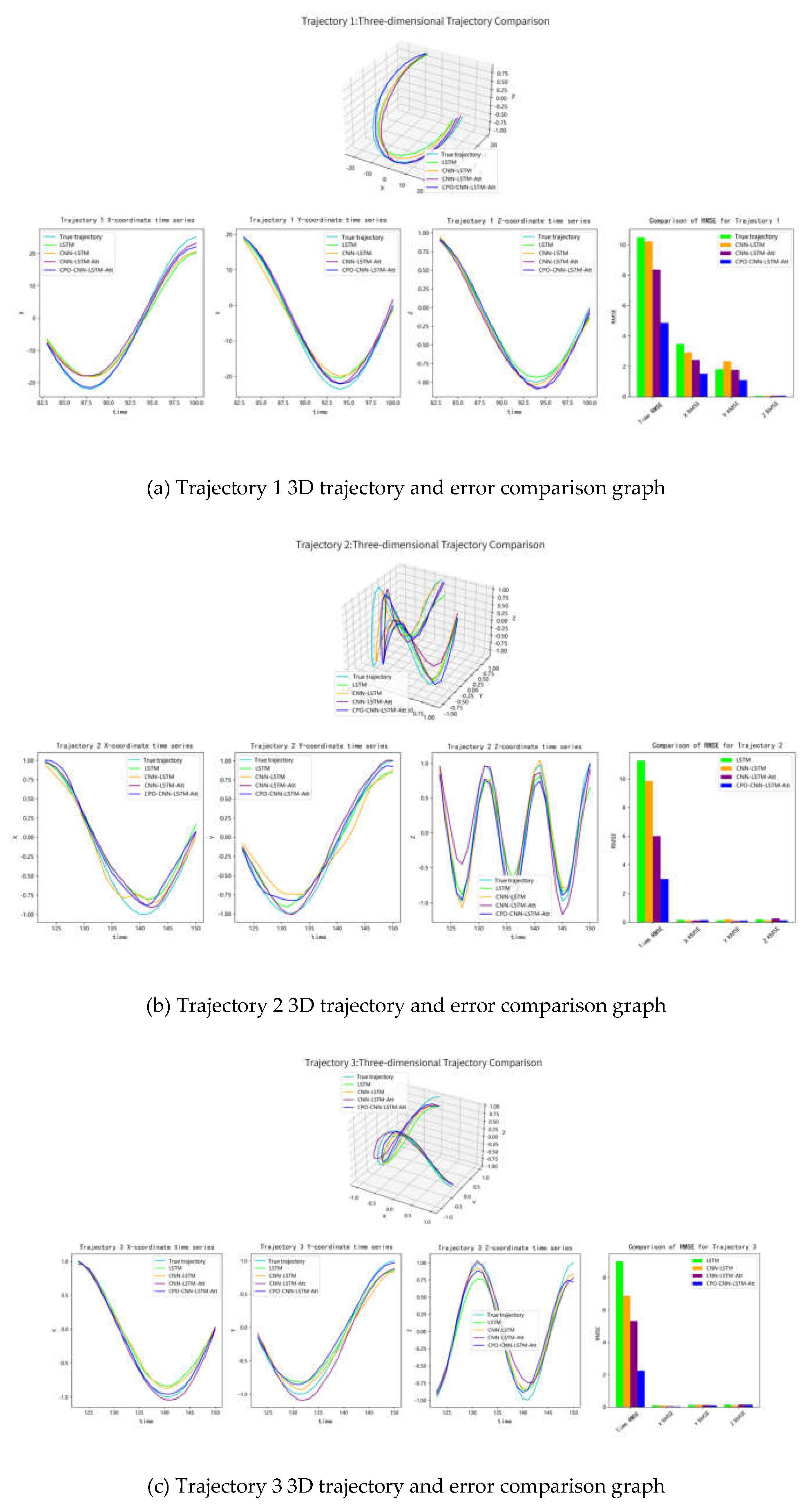
To further evaluate the predictive performance of the models, this study compared the predictive performance of four models (LSTM, CNN-LSTM, CNN-LSTM-Attention, and CPO-CNN-LSTM-Attention) on trajectories 1, 2, and 3. Figures 9 (a), 9 (b), and 9 (c) respectively show the three-dimensional trajectory comparison of trajectory 1, trajectory 2, and trajectory 3, schematic diagrams of x, y, and z coordinates over time, and the error index histograms of the four models.
Take Figure 9 (a) as an example. By comparing the 3D trajectory graphs in the figure, it can be seen intuitively that the C-CLA model fits the best, and the curves it draws in the test set almost coincide with the real trajectory. The rest of the models all have some errors in the prediction process, among which the LSTM model deviates the most from the real trajectory. Through the x, y, and z coordinate time series, the experimental results further show that the C-CLA model predicts the closest to the real trajectory in all directions, while the LSTM model and the CNN-LSTM model show greater deviations during the recovery phase. From the RMSE histogram, it can be seen that the overall RMSE of the C-CLA model is the lowest, while that of the LSTM model is the highest. In the X, Y, and Z directions, the RMSE of the C-CLA is significantly lower than that of other models.
Figures 9 (b) and 9 (c) show the predictions of trajectories 2 and 3, presenting a trend similar to that in Figure 9 (a). Trajectories 2 and 3 are more complex and contain more volatility, but the C-CLA model still shows the best predictive performance, with its predicted trajectories highly consistent with the real trajectories, and the overall RMSE remains around 2.
Overall, the C-CLA model outperforms other models on all trajectories, with its predicted trajectories being the closest to the real trajectories and having the lowest RMSE. The LSTM model had the poorest predictive performance, especially in the Z direction, indicating its insufficient ability to model complex trajectories. CPO optimizes two hyperparameters, the number of hidden layer neurons and the initial learning rate, for the LSTM model through population reduction techniques, resulting in smaller initial loss values, faster convergence, and optimal predictive performance during training.
Figure 9.
3D comparison of model prediction effect
4.6. Quantitative Analysis
The effectiveness of the trajectory prediction model proposed in this paper can be verified by quantitatively analyzing the error metrics of the C-CLA model relative to traditional deep learning trajectory prediction algorithms. In this section, quantitative experiments are conducted between the proposed C-CLA model and the traditional LSTM model. To reduce the impact of random errors on the analysis, RMSE, MAE, and MAPE are selected. The average error was calculated to analyze the accuracy of track prediction, and the visualization results of the error analysis are shown in Table 5 and Figure 10.
In terms of trajectory 1 prediction, the average RMSE of the C-CLA model in the X, Y, and Z directions decreased by 2.0697 compared to LSTM, representing a reduction of 52.35%. MAE decreased by 2.0913 compared to LSTM, which accounted for 57.12 percent; MAPE decreased by 4.4882% compared to LSTM, accounting for 30.11%; In particular, in the time dimension, the MAE of C-CLA was 4.1658, which was 5.8420 lower than that of LSTM and accounted for as much as 58.37%.
In trajectory 2 and trajectory 3 predictions, the error metrics showed the same trend as Trajectory 1. It is notable that as the complexity of the aircraft's motion state increases from trajectory 1 to Trajectory 3, the proportion of error reduction of C-CLA relative to LSTM gradually increases, indicating that the C-CLA model has a stronger ability to capture nonlinear complex trajectory motion characteristics compared to other traditional models and is more suitable for trajectory prediction of fighter aircraft.
5. Conclusions
To study the trajectory prediction algorithm in the fighter jet automatic collision avoidance system, this paper uses a deep learning model to optimize the hyperparameters in the CNN-LSTM-Attention model by introducing the CPO optimization algorithm, and uses the optimal parameters found by CPO to train and test three simulated fighter jet flight trajectories.
The results show that the initial loss function and convergence rate of the C-CLA model with the best hyperparameters found by CPO are the best in the comparison experiment, and the lowest loss value is consistently maintained. The superiority of the C-CLA model in trajectory fitting was qualitatively verified, and three metrics, RMSE, MAE, and MAPE, were selected for quantitative evaluation. The experimental results demonstrated that the C-CLA model had a significant reduction in error metrics compared to the LSTM model and performed well in prediction accuracy and feature extraction for complex tracks. Further research can be conducted in the following areas:
(1) By using databases such as JSBsim, the performance parameters of different models were obtained to further verify the generalization ability of the C-CLA model;
(2) Improve the C-CLA model, for example, by adding more mechanisms to the CPO algorithm to enhance the robustness of the model.
(3) Study the impact of multiple perturbation factors (such as enemy threats, weather factors, etc.) on the model's predictive ability.
Abbreviations
| CPO | Crested Porcupine Optimization |
| CNN | Convolutional Neural Network |
| LSTM | Long Short-Term Memory |
| CLA | CNN-LSTM-Attention |
| C-CLA | CPO-CNN-LSTM-Attention |
| CFIT | Controlled Flight Into Terrain |
| Auto-GCAS | Automatic Ground Collision Avoidance System |
| KF | Kalman Filter |
| HMM | Hidden Markov Model |
| RMSE | Root Mean Square Error |
| MAE | Mean Absolute Error |
| MAPE | Mean Absolute Percentage Error |
References
- Huang, S.X. Research on Predictive Ground Collision Avoidance Warning Algorithm for Helicopters. Ph.D. Thesis, Nanjing University of Aeronautics and Astronautics, Nanjing, China, 2021.
- Sun, Y.S. The U.S. Air Force F-35A Fighter Is Equipped with an Automatic Ground Collision Avoidance System. China Aviat. News 2019, 5 November, 005.
- Development and Application Research of Automatic Ground Collision Avoidance System for Modern Fighter Aircraft. Flight Dyn. 2020, 38, 1–6, . [CrossRef]
- Song, K.K.; Chen, Y. Overview of the Development of Automatic Ground Collision Avoidance System for U.S. Fighter Aircraft. Aviat. World 2017, 4, 54–57.
- Xu, Z.F.; Zeng, W.L.; Yang, Z. A Survey of Aircraft Trajectory Prediction Technology. Comput. Eng. Appl. 2021, 57, 65–74.
- Tang, C.Y.; Tang, J.; Zeng, M.J. Aircraft Flight Path Prediction Based on Kalman Filter. Mod. Inf. Technol. 2023, 7, 74–78.
- Chen, M.Q.; Fu, J.Y. Research on Flight Path Prediction Method Based on Unscented Kalman Filter. Comput. Simul. 2021, 38, 27–30, 36.
- Lymperopoulos, I.; Lygeros, R. Sequential Monte Carlo Methods for Multi-Aircraft Trajectory Prediction in Air Traffic Management. Int. J. Adapt. Control Signal Process. 2010, 24, 830–849, . [CrossRef]
- Wang, C.; Guo, J.X.; Shen, Z.P. 4D Trajectory Prediction Method Based on Basic Flight Model. J. Southwest Jiaotong Univ. 2009, 44, 295–300, . [CrossRef]
- Du, Z.M.; Zhang, J.F.; Miao, H.L.; et al. Prediction of Aircraft Continuous Climb Vertical Profile Considering Thrust Intention. J. Beijing Univ. Aeronaut. Astronaut. 2024, 50, 1347–1353, . [CrossRef]
- Zhang, X.; Han, Y. Research on Climb Performance and 4D Trajectory Prediction of Aircraft. In Proceedings of the 2013 International Conference on Computer Sciences and Applications, Wuhan, China, 14–15 deci 2013; pp. 390–393.
- Suplisson, A.W. Optimal Recovery Trajectories for Automatic Ground Collision Avoidance Systems (Auto GCAS). Master’s Thesis, United States Air Force Academy, Colorado Springs, CO, USA, 2015.
- Payeur, H.; Le-Huy, H.; Gosselin, C.M. Trajectory Prediction for Moving Objects Using Artificial Neural Networks. IEEE Trans. Ind. Electron. 1995, 42, 147–158, . [CrossRef]
- Williams, R.J.; Zipser, D. A Learning Algorithm for Continually Running Fully Recurrent Neural Networks. Neural Comput. 1989, 1, 270–280, . [CrossRef]
- Altché, F.; de La Fortelle, A. An LSTM Network for Highway Trajectory Prediction. In Proceedings of the IEEE 20th International Conference on Intelligent Transportation Systems (ITSC), Yokohama, Japan, 16–19 October 2017; pp. 353–359.
- Kim, B.; Kang, C.M.; Kim, J.; et al. Probabilistic Vehicle Trajectory Prediction over Occupancy Gridmap via Recurrent Neural Network. In Proceedings of the IEEE 20th International Conference on Intelligent Transportation Systems (ITSC), Yokohama, Japan, 16–19 October 2017; pp. 399–404.
- Zhang, Z.; Yang, R.; Fang, Y. LSTM Network Based on Antlion Optimization and Its Application in Flight Trajectory Prediction. In Proceedings of the 2018 2nd IEEE Advanced Information Management, Communicates, Electronic and Automation Control Conference (IMCEC), Xi’an, China, 25–27 May 2018; pp. 1658–1662.
- Dai, L.C.; Liu, X.; Zhang, H.Y.; et al. Flight Target Trajectory Prediction Based on Kalman Filter Algorithm. Syst. Eng. Electron. 2023, 45, 1814–1820, . [CrossRef]
- Wang, K.; Zhou, Z.C.; Qu, K.; et al. Trajectory Prediction Based on CNN-LSTM Model with Attention Mechanism. J. Air Force Eng. Univ. 2023, 24, 50–57.
- Abdel-Basset, M.; Mohamed, R.; et al. Crested Porcupine Optimizer: A New Nature-Inspired Metaheuristic. Knowl.-Based Syst. 2023, 284, 111257, . [CrossRef]
- Ahmad, M.A.; Al-Ja’afreh; Mokryani, G.; et al. An Enhanced CNN-LSTM Based Multi-Stage Framework for PV and Load Short-Term Forecasting: DSO Scenarios. Energy Rep. 2023, 10, 1387–1408, . [CrossRef]
- Ghimire, S.; Nguyen-Huy, T.; Deo, R.C.; Casillas-Pérez, D.; Salcedo-Sanz, S. Efficient Daily Solar Radiation Prediction with Deep Learning 4-Phase Convolutional Neural Network, Dual Stage Stacked Regression and Support Vector Machine CNN-REGST Hybrid Model. Sustain. Mater. Technol. 2022, 32, e00429, . [CrossRef]
- Ehteram, M.; Afshari Nia, M.; Panahi, F.; Farrokhi, A. Read-First LSTM Model: A New Variant of Long Short Term Memory Neural Network for Predicting Solar Radiation Data. Energy Convers. Manag. 2024, 305, 118267, . [CrossRef]
- Gao, B.; Huang, X.; Shi, J.; Tai, Y.; Zhang, J. Hourly Forecasting of Solar Irradiance Based on CEEMDAN and Multi-Strategy CNN-LSTM Neural Networks. Renew. Energy 2020, 162, 1665–1683, . [CrossRef]
Figure 1.
AGCAS module system architecture
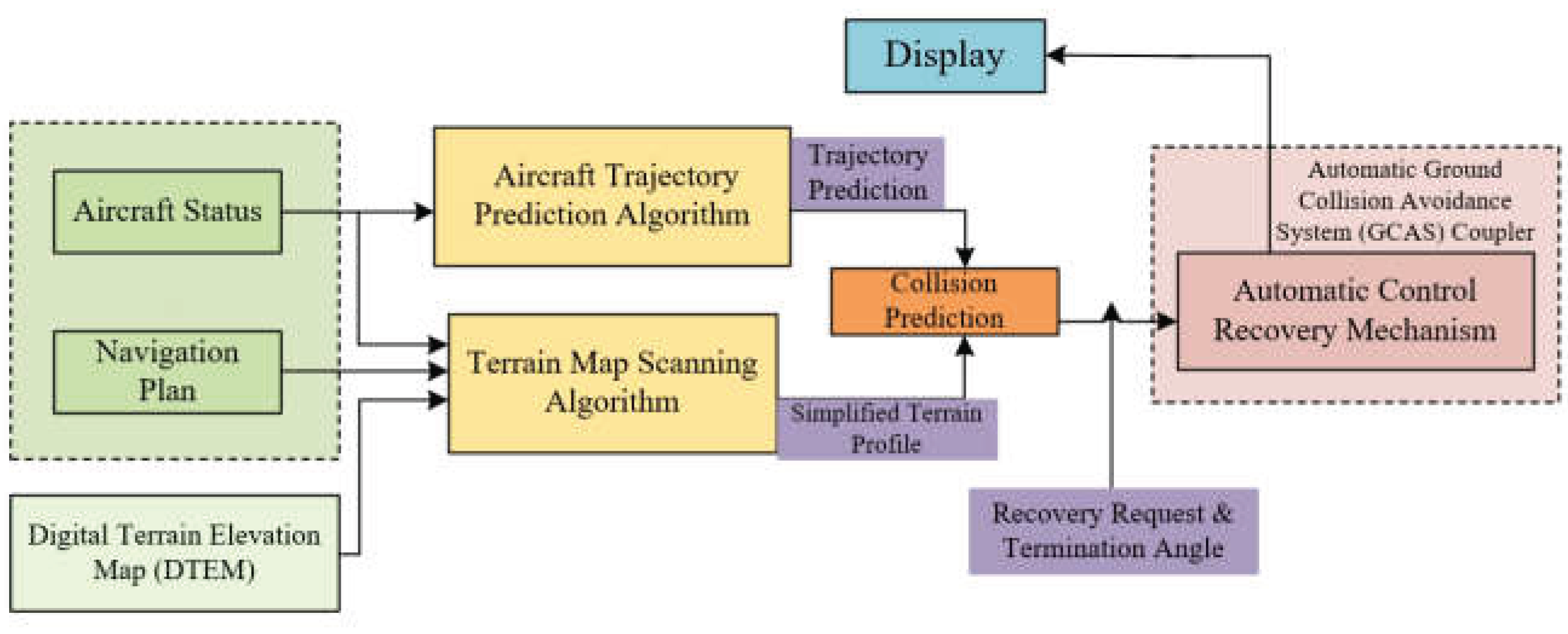
Figure 2.
One-dimensional convolutional neural networks learn time series features
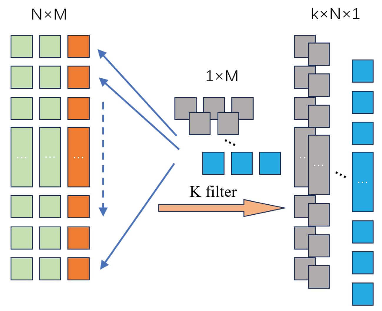
Figure 3.
The basic structure of the LSTM neural network
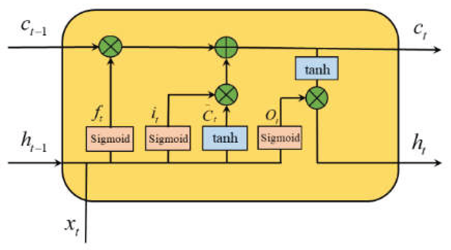
Figure 4.
Schematic Diagram of Multi-Head Attention Mechanism
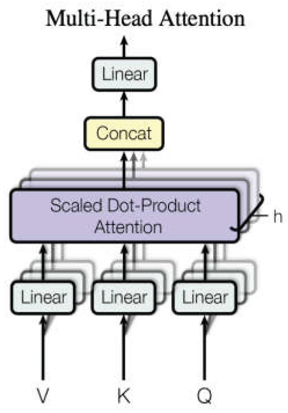
Figure 5.
C-CLA flight trajectory prediction model structure
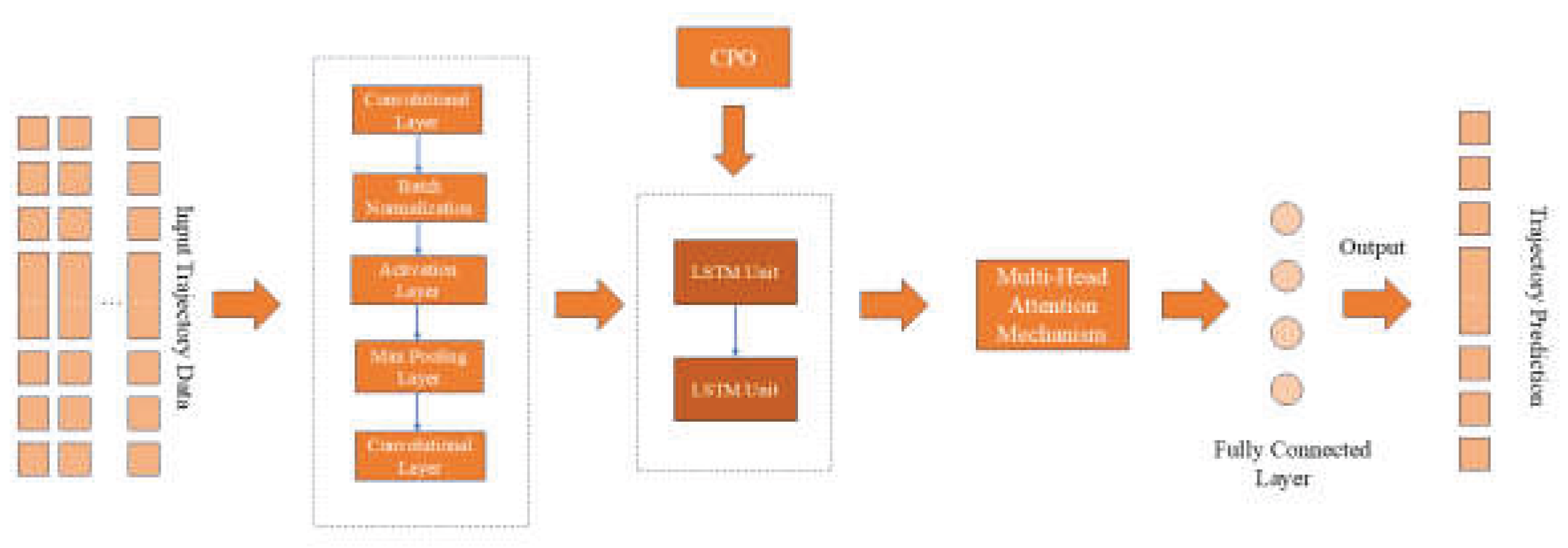
Figure 6.
Sample Structure Diagram
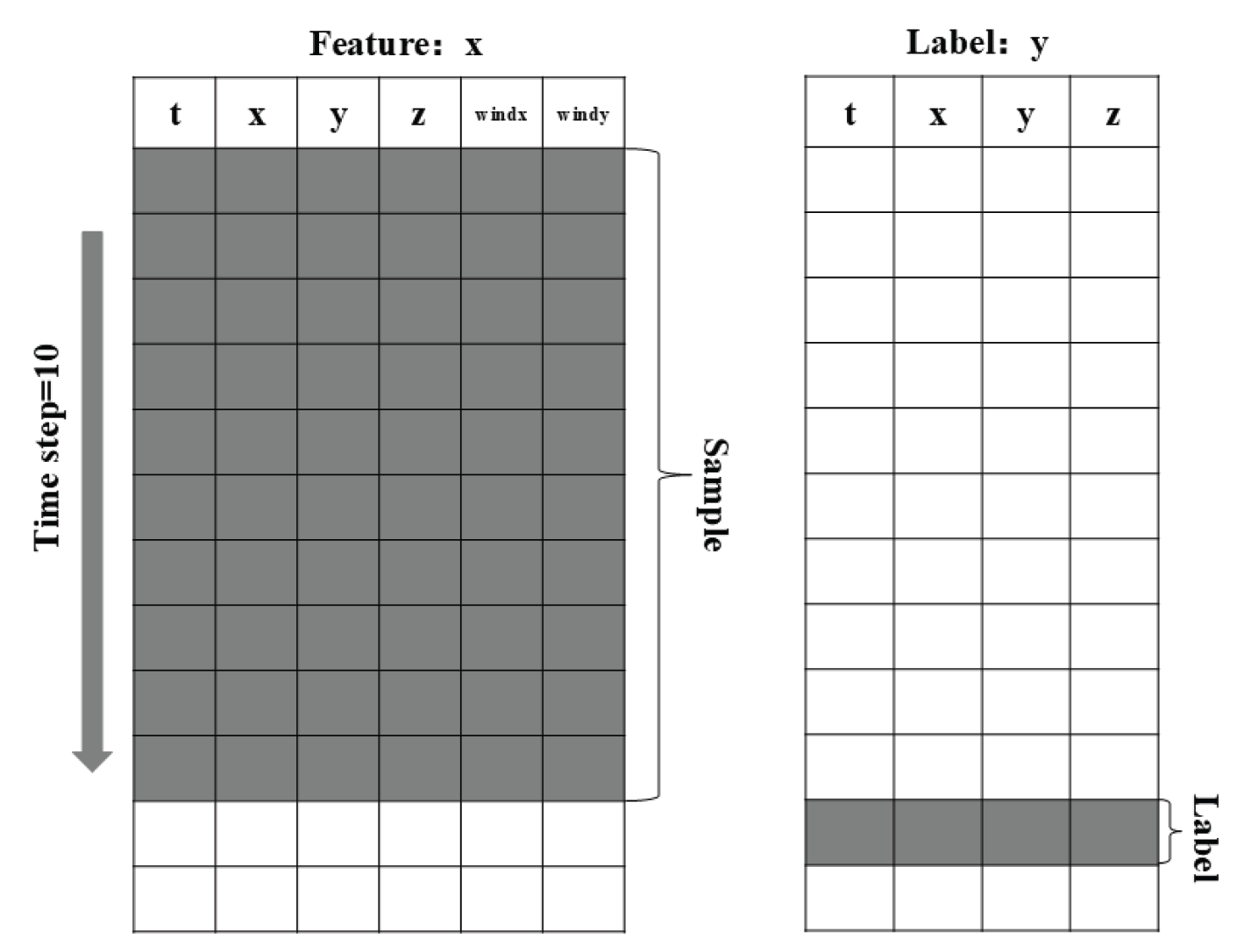
Figure 7.
C-CLA flight trajectory prediction model operation flow chart
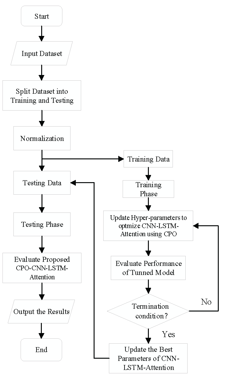
Figure 8.
Model loss function comparison diagram.
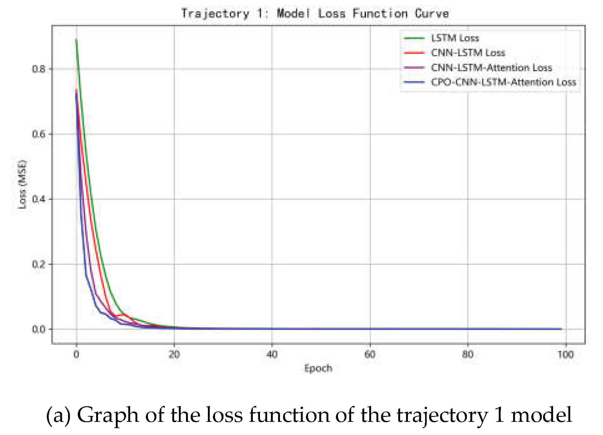
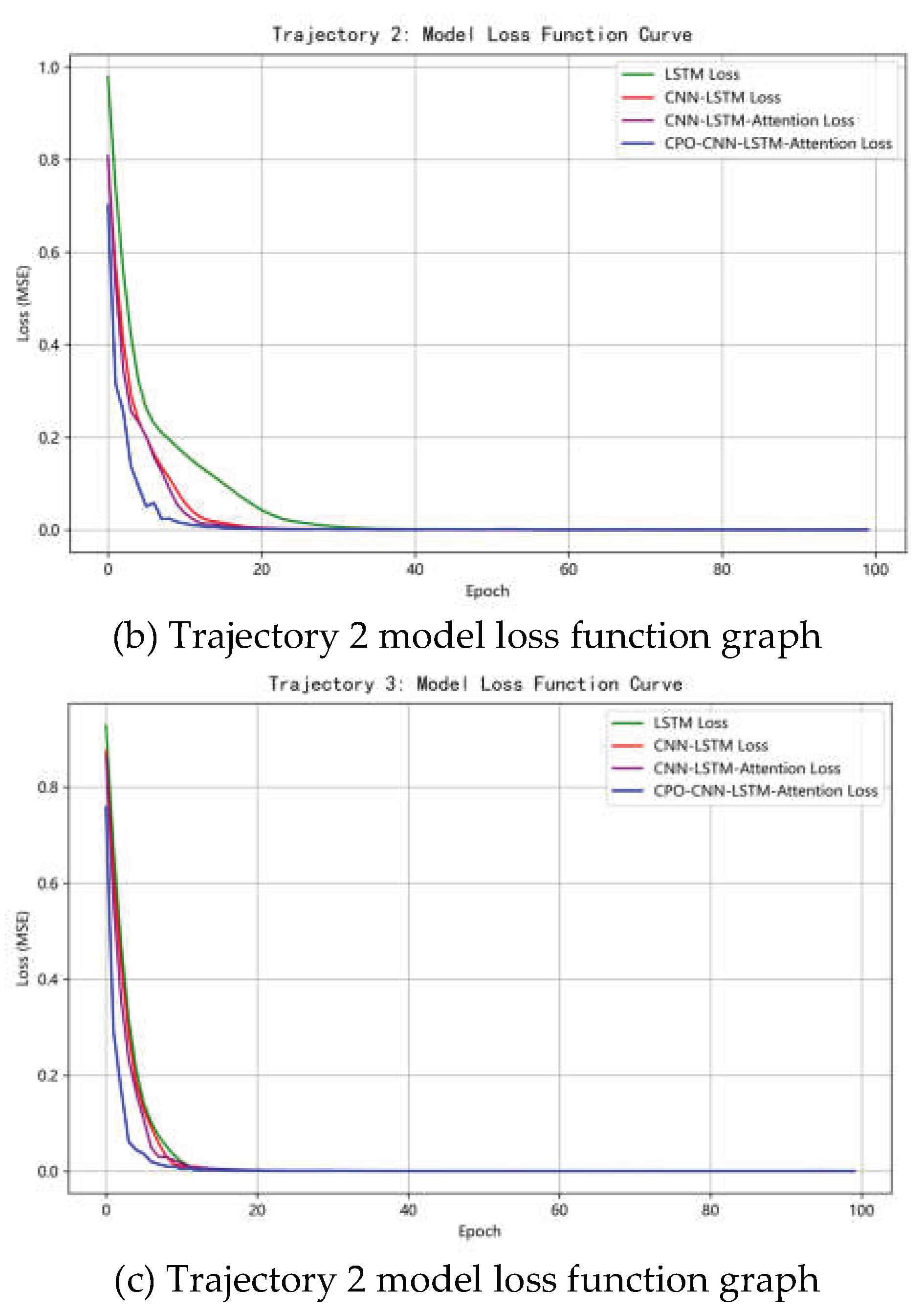
Figure 10.
Quantitative comparison between C-CLA model and LSTM model.
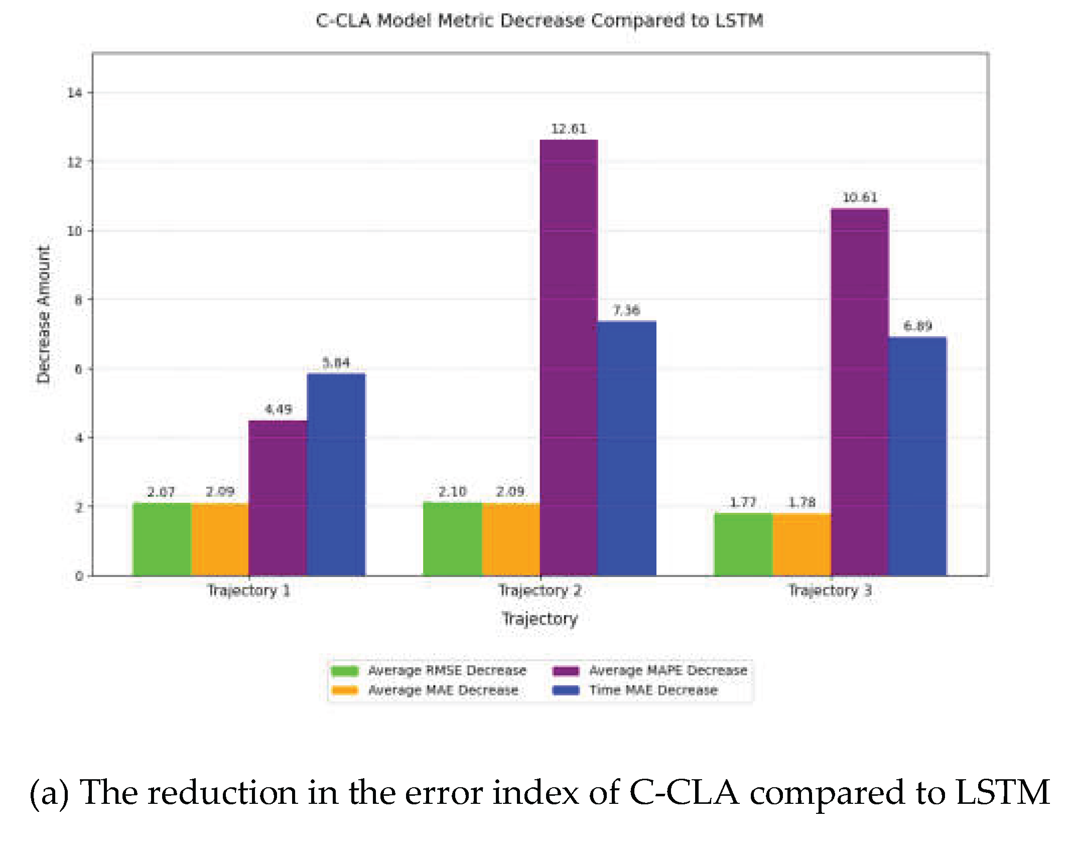
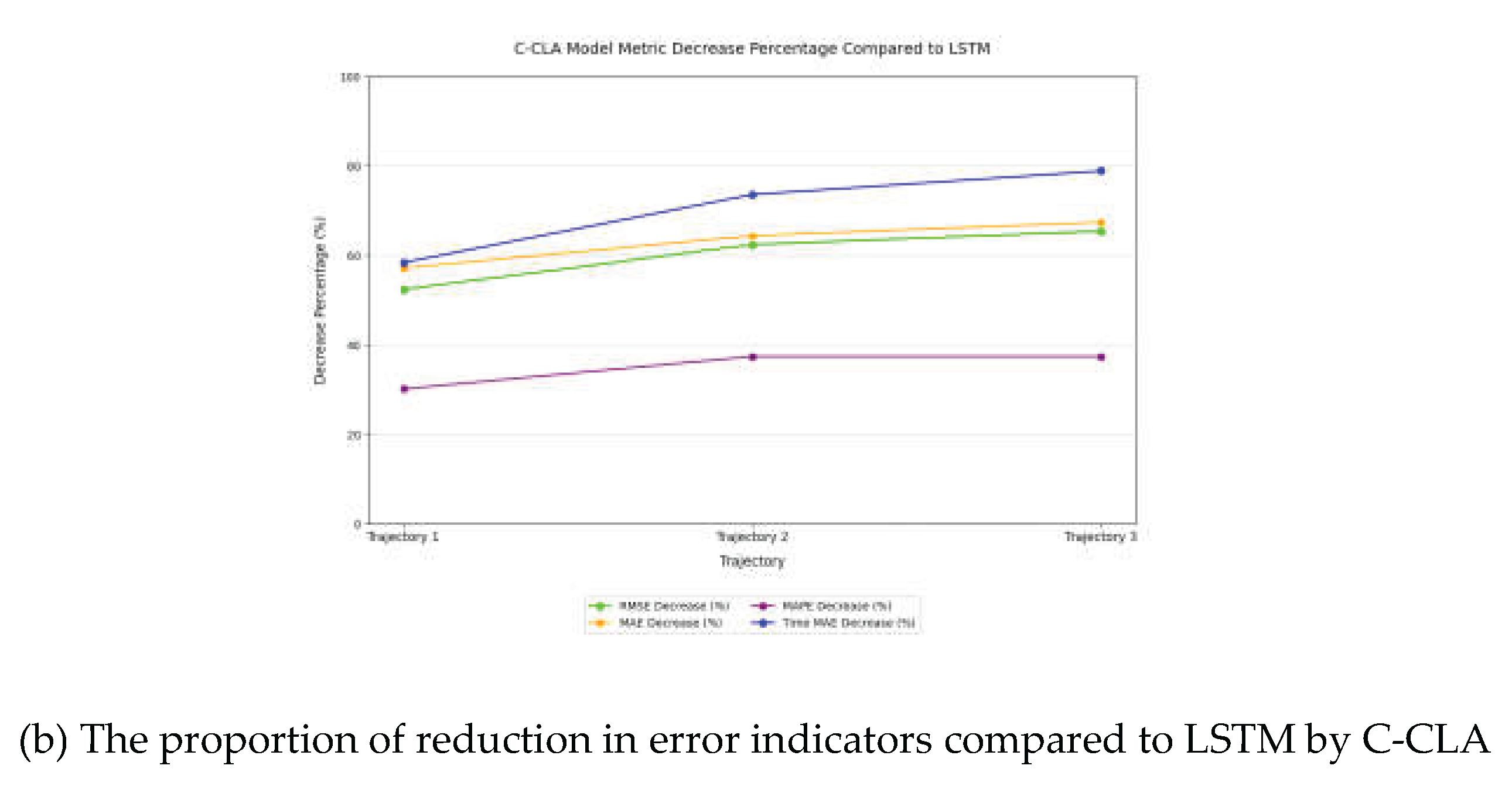

Table 1.
Simulated Aircraft Motion Trajectory Equations
| Simulation Data | Parametric Equation | Parameter Settings |
| 1 | ,200 time points | |
| 2 | ,300 time points | |
| 3 | ,300 time points |
Table 2.
Experimental Environment Configuration
| Category | Component | Description |
| Software | Development Tool | PyCharm 2024.1.1 (Professional Edition) |
| Operating System | Windows 11 | |
| Programming Language | Python 3.11.4 | |
| Framework | TensorFlow | |
| Hardware | Category | Processor13th Gen Intel® Core™ i7-13620H (10 cores/16 threads, 2.4 GHz to 4.9 GHz) |
| Memory | 16 GB DDR5 5200 MHz | |
| Graphics Card | NVIDIA GeForce RTX 4060 Laptop GPU (8 GB VRAM) | |
| Storage | 1 TB NVMe SSD |
Table 3.
Network Parameter Table.
| Model | Units | Learning Rate | Epochs |
| LSTM | 64 | 0.001 | 100 |
| CNN-LSTM | 64 | 0.001 | 100 |
| CNN-LSTM-Attention | 64 | 0.001 | 100 |
| CPO-CNN-LSTM-Attention | Optimised | Optimised | 100 |
Table 4.
Hyperparameters optimized by CPO.
| Best Hidden Nodes | Optimal learning rate | |
| Trajectory 1 | 32 | 0.0029 |
| Trajectory 2 | 78 | 0.0054 |
| Trajectory 3 | 100 | 0.0049 |
Table 5.
Reduction and percentage of C-CLA model relative to LSTM index.
| Trajectories | Indicators | Reduction amount | Decrease percentage (%) |
| Trajectory 1 | Average RMSE | 2.0697 | 52.35 |
| Average MAE | 2.0913 | 57.12 | |
| Average MAPE | 4.4882 | 30.11 | |
| Time MAE | 5.842 | 58.37 | |
| Trajectory 2 | Average RMSE | 2.0973 | 62.37 |
| Average MAE | 2.0935 | 64.37 | |
| Average MAPE | 12.6145 | 37.37 | |
| Time MAE | 7.3606 | 73.55 | |
| Trajectory 3 | Average RMSE | 1.7743 | 65.37 |
| Average MAE | 1.7755 | 67.37 | |
| Average MAPE | 10.6145 | 37.37 | |
| Time MAE | 6.8887 | 78.84 |
Disclaimer/Publisher’s Note: The statements, opinions and data contained in all publications are solely those of the individual author(s) and contributor(s) and not of MDPI and/or the editor(s). MDPI and/or the editor(s) disclaim responsibility for any injury to people or property resulting from any ideas, methods, instructions or products referred to in the 18content. |
© 2025 by the authors. Licensee MDPI, Basel, Switzerland. This article is an open access article distributed under the terms and conditions of the Creative Commons Attribution (CC BY) license (http://creativecommons.org/licenses/by/4.0/).
Copyright: This open access article is published under a Creative Commons CC BY 4.0 license, which permit the free download, distribution, and reuse, provided that the author and preprint are cited in any reuse.


