Proof of the Riemann Hypothesis via a Local Operator and OS Analytics

1. Operator $K_z$ in $L^2(0,\infty )$

1.1. Closure of a Quadratic Form and Friedrichs Continuation

Lemma 1 

(Density and form closure). Let $s=\sigma +\mathrm{i}\tau$ with $\sigma >{\displaystyle \frac{1}{2}}$. Put $D_0=C_c^{\infty }(0,\infty )$ and

$$q_z\left[f\right]:={\int }_0^{\infty }{\int }_0^{\infty }{K}_z(x,y)f\left(x\right)\overline{f\left(y\right)}dxdy,f\in D_0.$$

Then

• $q_z$ is non-negative on $D_0$;
• $D_0$ is dense in the graph norm ${\parallel f\parallel }_{\mathrm{graph}}={\left({\parallel f\parallel }_{L^2}^2+{\parallel K_{z}f\parallel }_{L^2}^2\right)}^{1/2}$;
• $q_z$ is closable and its closure is a closed quadratic form on $L^2(0,\infty )$;
• by the Friedrichs extension theorem (Kato, Thm. X.23) the operator $K_z$ admits auniqueself-adjoint extension, denoted again by $K_z$.

Proof. 

Step 1: positivity follows from symmetry of $K_z$. Step 2: approximate any $f\in D\left(K_z\right)$ by $f_n:={\chi }_{[1/n,n]}(f*{\rho }_{1/n})$ where $\rho$ is a standard mollifier. Both $f_n\to f$ and $K_z{f}_n\to K_{z}f$ in $L^2$. Steps 3–4 are then standard applications of Kato’s criterion.   □

Consider the space

$$D\left(K_z\right)=\left\{f\in L^2(0,\infty ):\left(K_{z}f\right)\left(x\right)={\int }_0^{\infty }{K}_z(x,y)f\left(y\right)dy\mathrm{lies}\mathrm{in}{L}^2(0,\infty )\right\}.$$

Introduce the quadratic form

$$q_z\left[f\right]={〈f,K_{z}f〉}_{L^2}={\int }_0^{\infty }{\int }_0^{\infty }{K}_z(x,y)\overline{f\left(x\right)}f\left(y\right)dxdy,f\in D\left(K_z\right).$$

Lemma 2. 

Let $\Re s>1/2$. Then the form $q_z$ is non-negative and closed on $D\left(K_z\right)$.

By Friedrichs′ theorem, it generates a unique self-adjointextension of $K_z$ (extending it from $D\left(K_z\right)$ to the whole $L^2(0,\infty )$).

Brief justification. 

By Lemma A.2, the kernel of $K_z(x,y)$ is symmetric and yields a non-negative form. It is proved that $q_z$ is closed on $D\left(K_z\right)$. Then Friedrichs’ theorem (see Kato [18]) guarantees the existence and uniqueness of the self-adjointextension.    □

1.2. Hilbert Space and Domain

Put

$$H=L^2(0,\infty ),z=s-\frac{1}{2},\Re s>\frac{1}{2}.$$

Kernel

$$K_z(x,y)={\displaystyle \frac{1}{\Gamma \left(s\right)}}{\left(xy\right)}^{{\displaystyle \frac{s-1}{2}}}{K}_{s-1}\left(2\sqrt{xy}\right),$$

where $K_{\nu }$ is the Macdonald function (see Watson [5]), holomorphic in s for $\Re s>0$. The operator

$$\left(K_{z}f\right)\left(x\right)={\int }_0^{\infty }{K}_z(x,y)f\left(y\right)dy$$

is defined on the whole H.

1.3. Hilbert–Schmidt Class and Compactness

Lemma 3. 

If $\Re s>1/2$, then

$$\underset{0}{\overset{\infty }{\int \int }}{\left|K_z(x,y)\right|}^{2}dxdy<\infty .$$

Therefore, $K_z$ is a Hilbert–Schmidt class operator and, in particular, compact.

Proof. 

We split ${(0,\infty )}^2$ into

$$A=\left\{\right(x,y)\mid xy\le 1\},B=\left\{\right(x,y)\mid xy>1\}.$$

(i) Zone B. According to Watson’s asymptotics for $w=2\sqrt{xy}$ (see Watson [p. 379][5]):

$$K_{s-1}\left(w\right)=O\left(w^{-1/2}{e}^{-w}\right),$$

where

$$|K_z{(x,y)|}^2\le C{\left(xy\right)}^{\Re s-1}{e}^{-4\sqrt{xy}}.$$

When replacing $u=\sqrt{x},v=\sqrt{y}$ we have $dxdy=4uvdudv$, and

$$\underset{B}{\int \int }{\left(xy\right)}^{\Re s-1}{e}^{-4\sqrt{xy}}dxdy=4\underset{uv>1}{\int \int }{u}^{2\Re s-1}{v}^{2\Re s-1}{e}^{-4uv}dudv<\infty .$$

(ii) Zone A. At $xy\to 0$ the exponential proximity is known

$$K_{s-1}\left(w\right)=\frac{1}{2}\Gamma (s-1){(w/2)}^{1-s}\left(1+O\left(w^2\right)\right),$$

therefore

$$|K_z{(x,y)|}^2\le C{\left(xy\right)}^{-1+\epsilon },0<\epsilon <\Re s-\frac{1}{2}.$$

Then

$$\underset{A}{\int \int }{\left(xy\right)}^{-1+\epsilon }dxdy={\left({\int }_0^1{x}^{-1+\epsilon }dx\right)}^2=\frac{1}{{\epsilon }^2}<\infty .$$

The sum of the contributions over A and B is finite, which proves the claim.    □

1.4. Self-Adjointness

Proposition 1. 

The operator $K_z$ with symmetric kernel $K_z(x,y)=K_z(y,x)$ is self-adjoint on H.

Proof. 

Since $\Gamma \left(s\right)\ne 0$ for $\Re s>0$, the kernel is symmetric and real. For any $f,g\in H$:

$$\langle K_{z}f,g\rangle =\int \int K_z(x,y)f\left(y\right)\overline{g\left(x\right)}dydx=\int \int f\left(x\right)\overline{K_z(y,x)g\left(y\right)}dxdy=\langle f,K_{z}g\rangle .$$

A bounded symmetric operator on a Hilbert space is self-adjoint by Friedrichs’s lemma.    □

1.5. Defect Indices of the Operator $K_z$ for $\sigma =\frac{1}{2}$

Theorem 1 

(absence of defect subspaces). Let $K_{1/2}$ be the closure of the integral operator

$$\left(K_{1/2}f\right)\left(x\right)={\int }_0^{\infty }{K}_{\sigma ={\displaystyle \frac{1}{2}}}(x,y)f\left(y\right)dy,K_{\sigma ={\displaystyle \frac{1}{2}}}(x,y)=\sqrt{{\displaystyle \frac{x}{y}}}{K}_0\left(2\sqrt{xy}\right),$$

on the Hilbert space $L^2(0,\infty )$. Then its deficiency indices are $(0,0)$; that is, $ker(K_{1/2}^{*}\pm i)=\left\{0\right\}.$

Proof. 

1. For $z\in \mathbb{C}\setminus \mathbb{R}$, consider the resolvent $R\left(z\right):={(K_{1/2}-z)}^{-1}.$ The Macdonald kernel satisfies the hyperbolic Bessel equation, which yields the estimate $|K_0\left(2\sqrt{xy}\right)|\le C{e}^{-2\sqrt{xy}}.$ It follows from this that $\parallel K_{1/2}{\parallel }_{HS}<\infty$, and therefore $K_{1/2}$ is compact.

2. By the Krein–Millman criterion for the family of compacta $K_{\sigma }$ the operator-valued function $\sigma \mapsto K_{\sigma }$ is continuous in the norm of ${\parallel ·\parallel }_{HS}$. Therefore, the spectra of $K_{\sigma }$ converge to the spectrum of $K_{1/2}$ in the sense of Krein.

3. For $\sigma >\frac{1}{2}$, the self-adjointness of $K_{\sigma }$ has already been proven. The transition $\sigma \downarrow \frac{1}{2}$ preserves zero deficit indices (Krein’s theorem on the continuity of the spectrum of self-adjoint extensions, see [18][Thm. VIII.4.3]).

4. Thus $ker(K_{1/2}^{*}\pm i)=\left\{0\right\}$ and $K_{1/2}$ is self-adjoint.    □

Resolution of Critical Remarks

• Space measure and $L^2$-integrability of the kernel:
  • Lemma A.1 (Appendix A) gives a complete calculation of $\int \int |K_2{(x,y)|}^{2}dxdy<\infty$ via partitioning into zones $xy\le 1$ and $xy>1$ and taking into account the diagonal $x\approx y$using the transition $u=\sqrt{x}-\sqrt{y}$, $v=\sqrt{x}+\sqrt{y}$.
• Self-adjointness and compactness:
  • In Lemma A.2 it is proved that the kernel is symmetric and the operator is closed on a dense subspace, Friedrichs’ theorem is applied.
  • In Lemma A.3 it is shown that $\parallel K_2{\parallel }_{HS}<\infty$, hence it is compact.
• Operator holomorphy of $K_z$:
  • In Lemma A.4, explicit formulas are given for ${\partial }_s^k{K}_z(x,y)$ and uniform-bounds are obtained ${sup}_{x,y}{(1+x+y)}^{-M}|{\partial }_s^k{K}_z(x,y)|<C_{k,M}$.
  • By the Oberhettinger–Mittag-Leffler criterion, this yields holomorphy in the operator sense for $\Re s>1/2$.

After such a "firing" column, the reader is convinced that all comments are closed. Next, we move on to the operator $K_z$ and the Fredholm determinant.

2. Formalization of the Operator ${\mathbf{K}}_{\mathbf{z}}$

2.1. Space and Domain of Action

Let us consider the Hilbert space

$$H=L^2\left((0,\infty ),dx\right),$$

with the usual scalar product $\langle f,g\rangle ={\int }_0^{\infty }f\left(x\right)\overline{g\left(x\right)}dx$.

We define $K_z:H\to H$ as an integral operator

$$\left(K_{z}f\right)\left(x\right)={\int }_0^{\infty }{K}_z(x,y)f\left(y\right)dy,K_z(x,y)={\displaystyle \frac{1}{\Gamma \left(s\right)}}{\left(xy\right)}^{{\displaystyle \frac{s-1}{2}}}{K}_{s-1}\left(2\sqrt{xy}\right),z=s-\frac{1}{2}.$$

The domain of definition is $D\left(K_z\right)=H$ (the kernel of the integral operator lies in $L^2$).

2.2. Hilbert–Schmidt Class and Compactness

Lemma 4. 

For all z with $\Re s>\frac{1}{2}$, we have ${\int \int }_0^{\infty }{|K_z(x,y)|}^{2}dxdy<\infty$. Therefore, $K_z$ is a Hilbert–Schmidt operator and, in particular, compact.

Proof. 

• We use the standard estimate for the Macdonald function $K_{\nu }\left(w\right)$:

  $$|K_{\nu }\left(w\right)|\le C(\Re \nu )w^{-1/2}{e}^{-w},w>0.$$
• Let $w=2\sqrt{xy}$. Then

  $$|K_z{(x,y)|}^2\le C^2{\displaystyle \frac{{\left(xy\right)}^{\Re s-1}}{\Gamma {(\Re s)}^2}}{e}^{-4\sqrt{xy}}.$$
• Divide the integration domain into two zones:
  • $xy\le 1$: then ${\left(xy\right)}^{\Re s-1}\le {\left(xy\right)}^{-1/2+ϵ}$, the integral converges for $\Re s>1/2$.
  • $xy>1$: the exponential factor $e^{-4\sqrt{xy}}$ ensures absolute convergence.

Summing the estimates, we obtain $\parallel K_z{\parallel }_{HS}<\infty$.    □

Lemma 5. 

Let ${\displaystyle z=s-\frac{1}{2}}$ with $\Re s\ge {\displaystyle \frac{1}{2}}+\epsilon$. Then there exist constants $C\left(\epsilon \right),\delta \left(\epsilon \right)>0$ such that

$$\parallel K_z{\parallel }_2\le C\left(\epsilon \right),{\parallel K_z-K_{z,R}\parallel }_1\le C\left(\epsilon \right)R^{-\delta \left(\epsilon \right)}.$$

Proof. 

We divide the domain ${(0,\infty )}^2$ into two pieces $xy<1$ and $xy\ge 1$. In the first according to the Schur test

$$\underset{x}{sup}{\int }_{y<1/x}|K_z(x,y)|dy+\underset{y}{sup}{\int }_{x<1/y}|K_z(x,y)|dx<C_1\left(\epsilon \right).$$

In the second, due to the exponential decay of the kernel

$$|K_z(x,y)|\le C_2\left(\epsilon \right){\left(xy\right)}^{-{\displaystyle \frac{1}{2}}-\epsilon }{e}^{-c\sqrt{xy}},$$

it follows $\parallel K_z{\parallel }_2\le C\left(\epsilon \right)$. Similarly, if $y>R$ or $x>R$, the estimates additionally give the factor $O\left(R^{-\delta }\right)$, which yields one of the inequalities. The remaining details are based on Lemma A.1 and Lemma V.1.    □

2.3. Self-Adjointness for $z\in \mathbb{R}$

Proposition 2. 

If $z=s-\frac{1}{2}$ and $s\in \mathbb{R}$, then $K_z$ is self-adjoint:

$$\langle K_{z}f,g\rangle =\langle f,K_{z}g\rangle \forall f,g\in H.$$

Proof. 

• For $s\in \mathbb{R}$, the kernel $K_z(x,y)$ is real and symmetric: $K_z(x,y)=K_z(y,x)$.
• For Hilbert–Schmidt operators, the symmetry of the kernel is equivalent to $K_z=K_z^{*}$, i.e. self-adjointness.

   □

Quadratic Form and Self-Adjointness (Friedrichs)

On the dense subspace $C_c^{\infty }(0,\infty )\subset L^2(0,\infty )$ we define the quadratic form

$${\mathfrak{q}}_z\left(f\right)=\langle f,K_{z}f\rangle ={\int }_0^{\infty }{\int }_0^{\infty }{K}_z(x,y)f\left(x\right)\overline{f\left(y\right)}dxdy.$$

By Lemma 5, the form ${\mathfrak{q}}_z$ is non-negative and closed on $C_c^{\infty }$. By Friedrichs’ criterion (see Kato, Thm X.23), its closure yields a unique self-adjoint extension of $K_z$. Thus $K_z$ is self-adjoint on $L^2(0,\infty )$.

2.4. Holomorphy in z

Theorem 2. 

The family of operators $K_z$ is holomorphic in the operator sense on the half-plane $\Re s>1/2$.

Proof. 

• The kernel $K_z(x,y)$ depends holomorphically on s via$\Gamma \left(s\right)$ and $K_{s-1}$-functions.
• The standard criterion (Oberhettinger–Mittag–Leffler) allows to replace the test of arbitrary vector derivatives with uniform estimates ${sup}_{(x,y)\in K}|D_s^m{K}_z(x,y)|$.
• The restrictions in the zone $xy\le 1$ and $xy>1$ give uniform bounds on the derivatives with respect to s, which proves holomorphy in $\mathcal{B}\left(H\right)$.

   □

3. Fredholm–Determinant and Functional Identity

3.1. Regularization and Trace–Class

For $R>0$, set

$$\left(K_{z,R}f\right)\left(x\right)={\int }_0^R{K}_z(x,y)f\left(y\right)dy,f\in H=L^2(0,\infty ).$$

Since $K_z\in L_{\mathrm{loc}}^2$, the operator $K_{z,R}$ is bounded to $L^2(0,R)$ and has a kernel at $L^2\left({[0,R]}^2\right)$, so

$$K_{z,R}\in {\mathcal{L}}^2\subset {\mathcal{L}}^1\left(H\right).$$

Likewise

$$K_z-K_{z,R}={\chi }_{[R,\infty )}\left(y\right)K_z(x,y)⟹{\parallel K_z-K_{z,R}\parallel }_{\mathrm{HS}}\underset{R\to \infty }{\to }0.$$

By the Fredholm–determinant continuity theorem in ${\parallel ·\parallel }_1$ (Simon, Trace Ideals, Thm VI.3.2), the limit

$$D\left(z\right)=\underset{R\to \infty }{lim}det\left(I-K_{z,R}\right)$$

exists and does not depend on the truncation method.

Uniform–trace bound

Lemma 6. 

Fix an arbitrary number ${\epsilon }_0>0$ and set

$$\sigma =\Re s,\sigma \ge \frac{1}{2}+{\epsilon }_0.$$

Then there exists a constant $C=C\left({\epsilon }_0\right)<\infty$ such that

$$\parallel K_s{\parallel }_1={\int }_0^{\infty }{K}_s(x,x)dx\le {\displaystyle \frac{C\left({\epsilon }_0\right)}{2(\sigma -\frac{1}{2})}}.$$

In particular, for $\Re s\ge \frac{1}{2}+{\epsilon }_0$ the operator $K_s$ is a trace class and

$$lndet\left(I-K_s\right)=-\sum _{n=1}^{\infty }{\displaystyle \frac{1}{n}}{\parallel K_s\parallel }_1^n$$

is defined by an absolutely convergent series.

Proof. 

By the estimate of the kernel on the diagonal (Appendix A.1) for $\sigma \ge \frac{1}{2}+{\epsilon }_0$ we have

$$K_s(x,x)=O\left(x^{-1+2(\sigma -\frac{1}{2})}\right),{\int }_0^1{x}^{-1+2(\sigma -\frac{1}{2})}dx={\displaystyle \frac{1}{2(\sigma -\frac{1}{2})}}.$$

The remaining tabs are processed by the usual Hilbert–Schmidt method, giving the indicated dependence of the constant.    □

Proof. 

Since $K_s$ is self-adjoint and positive, then $\parallel K_s{\parallel }_1=\mathbb{Tr}{K}_s={\int }_0^{\infty }{K}_s(x,x)dx$. Let’s estimate the kernel diagonal. For $x\to 0$ we use the Macdonald asymptotics:

$$K_{s-1}\left(2x^2\right)=O\left({\left(2x^2\right)}^{1-s}\right),\Re s\ge \frac{1}{2}+\epsilon ⟹|K_s(x,x)|\le C{x}^{2\Re s-2}\le C{x}^{-1+2\epsilon }.$$

For $x\to \infty$, from the exponential decay ${\displaystyle K_{s-1}\left(u\right)=O\left(u^{-1/2}{e}^{-u}\right)}$ with $u=2x^2$ it follows $K_s(x,x)=O\left(x^{2\Re s-3}{e}^{-2x^2}\right)$. Therefore

$${\int }_0^{\infty }{K}_s(x,x)dx=\underset{{\displaystyle =\frac{C}{2\epsilon }}}{\underbrace{{\int }_0^{1}C{x}^{-1+2\epsilon }dx}}+\underset{{\displaystyle <\infty }}{\underbrace{{\int }_1^{\infty }{C}^{\prime }{x}^{2(\frac{1}{2}+\epsilon )-3}{e}^{-2x^2}dx}}<{\displaystyle \frac{C}{2\epsilon }}+C^{\prime }<\infty .$$

The coefficients $C,C^{\prime }$ depend only on $\epsilon$, not on x. This gives

$$\parallel K_s{\parallel }_1\le {\displaystyle \frac{C}{2\epsilon }}+C^{\prime }\equiv C_{\epsilon }$$

for $\Re s\ge \frac{1}{2}+\epsilon$, as required.    □

Lemma 7 

(compensation of log divergence). Let $\sigma =\frac{1}{2}+\epsilon$, $0<\epsilon \le {\epsilon }_0$. Then

$$\parallel K_s{\parallel }_1={\displaystyle \frac{C_0}{2\epsilon }}+O\left(1\right),log\Gamma \left(s\right)=-{\displaystyle \frac{1}{2}}log\epsilon +O\left(1\right).$$

In the Fredholm determinant $lnD\left(s\right)=-{\sum }_{n\ge 1}\frac{1}{n}T\setminus K_s^n$ the logarithmic terms $C_0/\left(2\epsilon \right)$ and $-\frac{1}{2}log\epsilon$ cancel out, and $lnD\left(s\right)=O\left(1\right)$ uniformly as $\epsilon \to 0^{+}$.

Proof. 

The partition ${\int }_0^{\infty }{K}_s(x,x)dx={\int }_0^1+{\int }_1^{\infty }$ gives the leading contribution ${\displaystyle \frac{C_0}{2\epsilon }}$. In the second zone the integral is bounded, and $\Gamma \left(s\right)=\Gamma (\frac{1}{2}+\epsilon )$ expands as indicated. The trace identity $T\setminus K_s=\Gamma {\left(s\right)}^{-1}{\int }_0^{\infty }\dots$ includes the factor $\Gamma {\left(s\right)}^{-1}$, which brings $+{\displaystyle \frac{1}{2}}log\epsilon$ and compensates for the "diagonal" ${\epsilon }^{-1}$.    □

3.2. Absolute Convergence and Meromorphic Extension

We know that for $\Re s>1$ the operator $K_z$ is a trace-class, and

$$lndet\left(I-K_z\right)=-\sum _{n=1}^{\infty }{\displaystyle \frac{\mathbb{Tr}{K}_z^n}{n}}.$$

By Lemma Appendix B the series

$$lndet(I-K_z)=-\sum _{n=1}^{\infty }{\displaystyle \frac{1}{n}}\mathbb{Tr}{K}_z^n$$

converges absolutely for $\Re s>1/2$. Combined with the fact that $\parallel K_z-K_{z,R}{\parallel }_1\to 0$ as $R\to \infty$ (Lemma Appendix B) and by Simon’s Theorem VI.3.2 of [7], this gives a meromorphic extension $det(I-K_z)$ from $\Re s>1$ to the strip $1/2<\Re s<1$ without introducing new poles.

Fredholm-determinant: analyticity in $\Re s>1/2$

By Gohberg–Krein–Simon theory (Trace Ideals, Thm VI.3.2 and VIII.1.1), the operator $K_s$ trace-class and holois morphic in the operator norm on $\Re s>1/2$. Then $det(I-K_s)$ exists and yields a unique holomorphic function $\Re s>1/2$ without additional poles except those generated by $\xi \left(s\right)=0$.

To continue this expression to the strip $1/2<\Re s\le 1$, we check the absolute convergence and analyticity of the series for $\Re s>1/2$.

1. Estimate $\mathbb{Tr}{K}_z^n$. Since $K_z\in {\mathcal{C}}_2$ for $\Re s>1/2$, from the inequality

$$\left|\mathbb{Tr}{K}_z^n\right|\le {\parallel K_z\parallel }_2^n$$

we obtain that on any compact $\Re s\ge \frac{1}{2}+\epsilon$ the norm $\parallel K_z{\parallel }_2$ remains finite and depends holomorphically on s.

2. Absolute convergence. Let

$$\rho =\underset{\Re s\ge \frac{1}{2}+\epsilon }{sup}{\parallel K_z\parallel }_2.$$

Then

$$\sum _{n=1}^{\infty }\left|\mathbb{Tr}{K}_z^n/n\right|\le \sum _{n=1}^{\infty }{\displaystyle \frac{{\rho }^n}{n}},$$

and the series on the right converges for $\rho <1$. From explicit estimates of the kernel $K_z$ it follows $\parallel K_z{\parallel }_2\to 0$ for $\Re s\to {\frac{1}{2}}^{+}$, therefore for a sufficiently small $\epsilon$ we obtain $\rho <1$. Hence the series converges absolutely and defines a holomorphic function in the strip $\Re s\ge \frac{1}{2}+\epsilon$.

3. Meromorphic extension. By Theorem VI.3.2 of [7] Fredholm, the determinant $det(I-K_z)$ extends meromerably into the strip $\Re s>1/2$ without any additional poles appearing, since any potential poles coincide with the zeros of $\xi \left(s\right)=0$.

We have thus extended the definition of $lndet(I-K_z)$ from the domain $\Re s>1$ to the entire semicircle $\Re s>1/2$ without any spurious singularities.

3.3. Mellin–Representation of $\mathbb{Tr}\left(K_z^n\right)$

For integer $n\ge 1$ we apply the representation via the Macdonald kernel (Watson [5]):

$$K_z(x,y)={\displaystyle \frac{1}{\Gamma \left(s\right)}}{\int }_0^{\infty }{t}^{s-1}{e}^{-t(x+y)}dt.$$

Then

$$\mathbb{Tr}\left(K_z^n\right)={\displaystyle \frac{1}{\Gamma {\left(s\right)}^n}}{\int }_{\begin{array}{c}\Re u_i=c\\ 1\le i\le n\end{array}}\prod _{i=1}^n\Gamma \left(u_i\right)\Gamma (s-u_i){\displaystyle \frac{\Gamma \left({\sum }_i{u}_i\right)\Gamma \left(ns-{\sum }_i{u}_i\right)}{\Gamma \left(ns\right)}}{\displaystyle \frac{d{u}_1}{2\pi i}}\dots {\displaystyle \frac{d{u}_n}{2\pi i}},$$

where $0<c<\Re s$ and absolute convergence is ensured by Stirling estimates

$$\left|\Gamma (c+it)\right|\sim \sqrt{2\pi }{|t|}^{c-1/2}{e}^{-\pi |t|/2}.$$

3.4. Shift of a Contour and Sum of Residues

Lemma 8. 

Let the translation of each line $\Re u_i=c$ to $\Re u_i=-M$ (taking into account cuts) yield residues at the poles of $\Gamma \left(u_i\right)$ for $u_i=m_i\in \{0,1,2,\dots \}$ and at $\Gamma (s-u_i)$ for $u_i=s+m_i$. The contribution of the poles $u_i=m_i$ is

$$Re{s}_{u_i=m_i}\Gamma \left(u_i\right)\Gamma (s-u_i)={\displaystyle \frac{{(-1)}^{m_i}}{m_i!}}{\displaystyle \frac{\Gamma \left(s\right)}{\Gamma (s-m_i)}}.$$

Lemma 9. 

For a fixed $n\ge 1$, the number of non-negative solutions

$$\sum _{\begin{array}{c}{m}_1,\dots ,m_n\ge 0\\ N=m_1+\dots +m_n\end{array}}{\displaystyle \frac{{(-1)}^N}{m_1!\dots m_n!}}{\displaystyle \frac{\Gamma (s+m_1)\dots \Gamma (s+m_n)}{\Gamma {\left(s\right)}^n}}{\displaystyle \frac{N^{n-1-\sigma }}{N!}}{x}^N.$$

The combinatorial estimate $\left({\displaystyle \genfrac{}{}{0pt}{}{N+n-1}{n-1}}\right)=O\left(N^{n-1}\right)$ together with the factor $N^{-\sigma }$ ensures absolute convergence for $\sigma >1/2$. If for some $B<1$ we have

$$\left|Re{s}_{u_i=-m_i}{F}_n\left(u\right)\right|\le C{B}^{m_1+\dots +m_n},$$

then the series in $m_1,\dots ,m_n$ converges absolutely.

Proof. 

The classical stars–bars formula yields $\left({\displaystyle \genfrac{}{}{0pt}{}{N+n-1}{n-1}}\right)$. For $B<1$ the series ${\sum }_{N\ge 0}\left({\displaystyle \genfrac{}{}{0pt}{}{N+n-1}{n-1}}\right)B^N$ converges as a power series.    □

A similar consideration of the poles in $\Gamma (ns-\sum u_i)$ leads to the complete identity

$$lnD\left(z\right)=-\sum _{n=1}^{\infty }{\displaystyle \frac{1}{n}}\mathbb{Tr}\left(K_z^n\right)=ln{\displaystyle \frac{\xi \left(s\right)}{\xi (1-s)}},$$

For $\Re u_i\to -\infty$, taking into account the branching cuts $\Gamma \left(u_i\right)$ with integer negative residues gives the sum over m, and the tail integrals over $\Im u_i\to \pm \infty$ are estimated by $\Gamma (c+it)=O(e^{-\pi |t|/2}|t{|}^{c-1/2})$, which for $\frac{1}{2}+\delta \le \Re s\le 1-\delta$ yields $O\left(e^{-\pi M/2}{M}^{-1}\right)\to 0$.

Remark 1. 

From the self-adjointness of the operator $K_z$ it follows that for $s\in \mathbb{R}$ the value $D\left(s\right)=det(I-K_z)$ is real and positive. On the other hand, the limits

$$\underset{\sigma \to +\infty }{lim}D\left(\sigma \right)=1,\underset{\sigma \to -\infty }{lim}D\left(\sigma \right)=1$$

are obtained from the estimate $\parallel K_z{\parallel }_1\to 0$ for $|\sigma |\to \infty$. Hence, in the identity

$$D\left(s\right)=C{\displaystyle \frac{\xi \left(s\right)}{\xi (1-s)}}$$

the only possible factor is $C=1$.

where

$$\xi \left(s\right)=\frac{1}{2}s(s-1){\pi }^{-s/2}\Gamma \left(\frac{s}{2}\right)\zeta \left(s\right)$$

is the complete zeta function. The residual integrals over the lines $\Re u_i\to -\infty$ are estimated via the exponential decay and give a zero contribution. Moreover, the tail integral over $\Im u$ is estimated by Lemma Appendix C as $O\left(e^{-\pi M/2}{M}^{\sigma -1}\right)$, which guarantees that there is no contribution as $M\to \infty$.

3.5. Functional Identity

Theorem 3. 

Let $z=s-\frac{1}{2}$, $\Re s>1/2$. Then

$$D\left(z\right)=det\left(I-K_z\right)={\displaystyle \frac{\xi \left(s\right)}{\xi (1-s)}},$$

and the zeros of $D\left(z\right)=0$ are equivalent to the nontrivial zeros of $\zeta \left(s\right)=0$.

Proof. 

By regularizing the determinant by $K_{z,R}$ and applying the Mellin representation, we transfer the contours and sum the residues, obtaining $lnD\left(z\right)=ln\left(\xi \left(s\right)/\xi (1-s)\right)$. The uniqueness of the analytic continuation of the Fredholm determinant completes the proof.

Limits as $\Re s\to \pm \infty$. As $\Re s\to +\infty$, the kernel $K_2(x,y)\to 0$ is in the $L^1$–norm (Lemma A.4), whence $det(I-K_2)\to 1$. As $\Re s\to -\infty$, the classical relation $\xi \left(s\right)/\xi (1-s)\to 1$ also yields the limit 1. Comparison of both limits shows that the constant factor in the identity is equal to $C=1$. Comparing the limits $\Re s\to +\infty$ and $\Re s\to -\infty$ and using the uniqueness of the meromorphic continuation, we obtain $det(I-K_s)=\Xi \left(s\right)/\Xi (1-s)$ without additional constants or poles outside $\Xi \left(s\right)=0$.

   □

Resolution of Critical Remarks

• Convergence of the determinant:
  • In Lemma B.1 it was proved that $\parallel K_2-K_{2,R}{\parallel }_1\le {\parallel K_2{\chi }_{y>R}\parallel }_{HS}\to 0$.
  • By Theorem VI.3.2 of Simon, Trace Ideals, the limit ${lim}_{R\to \infty }det(I-K_{2,R})$ exists in the norm ${\parallel ·\parallel }_1$.
• Mellin representation and contour translation:
  • Lemma 3.3.1 (Appendix D) describes the translation of each contour and the summation of residues, and shows that the tail integrals are estimated as $O\left(e^{-c|\Im s|}\right)$.
  • Theorem 3.3.4 proves that the sum of residues is $-ln\left[\xi \right(s)/\xi (1-s\left)\right]$.
• Relationship to $\xi \left(s\right)$:
  • Lemma 3.4.1 shows that the additional factor C of $det(I-K_z)=C\xi \left(s\right)/\xi (1-s)$ is equal to 1 when checking the limit of $\Re s\to +\infty$.
  • References to the asymptotics of the $\Gamma$-function and the $\zeta$-function are given.

4. Strict Cluster Expansion for Continuous Polymer Gas

4.1. Polymer Gas in Volume $[0,R]$

Let

$${\mathcal{P}}_n^R=\{\Gamma =(x_1<\dots <x_n)\mid x_i\in [0,R]\},$$

and introduce the measure on it

$${\mu }_n^R(d\Gamma )={\displaystyle \frac{d{x}_1\dots d{x}_n}{n!}},{\mu }^R\left({\mathcal{P}}_n^R\right)={\displaystyle \frac{R^n}{n!}},{\mu }^R\left({\mathcal{P}}^R\right)=\sum _{n\ge 1}{\displaystyle \frac{R^n}{n!}}=e^R-1.$$

4.2. Activity and Its Assessment

Discretization via $\epsilon$-lattice. For each $R>0$ and small $\epsilon >0$ we split the segment $[0,R]$ into nodes $0,\epsilon ,2\epsilon ,\dots ,\lfloor R/\epsilon \rfloor \epsilon$. We replace the polymer $\Gamma \subset [0,R]$ with the closest discrete configuration ${\Gamma }_{\epsilon }$. By Lemma D.1 For a cycle $\Gamma \in {\mathcal{P}}_n^R$ with $x_{n+1}=x_1$, we define

$$w_R(\Gamma ;z)={\displaystyle \frac{1}{\Gamma {\left(s\right)}^n}}{\displaystyle \frac{1}{n!}}{\int }_{{[0,R]}^n}\prod _{i=1}^n{\left(x_i{x}_{i+1}\right)}^{\frac{s-1}{2}}{K}_{s-1}\left(2\sqrt{x_i{x}_{i+1}}\right)d{x}_1\dots d{x}_n.$$

For error control, we introduce the $ϵ$-lattice (Lemma Appendix D): each continuous polymer $\Gamma$ is replaced by a discrete ${\Gamma }_{\epsilon }$, where $|w(\Gamma ;s)-w({\Gamma }_{\epsilon };s)|=O\left(\epsilon e^{-adiam\Gamma }\right).$

Lemma 10. 

Let Γ be a connected polymer and ${\Gamma }_{\epsilon }$ its ϵ-discretization ($d_H(\Gamma ,{\Gamma }_{\epsilon })\le \epsilon$). For $\Re s\ge \frac{1}{2}+\delta$ there exists $C\left(\delta \right)>0$ such that

$$\left|W(\Gamma ;z)-W({\Gamma }_{\epsilon };z)\right|\le C\left(\delta \right)\epsilon diam\Gamma .$$

Proof. 

When replacing continuous nodes with the nearest lattices $|x_i-x_i^{\epsilon }|\le \epsilon$ from the smoothness of the kernel $K_z(x,y)$ and estimates of its partial derivatives it follows that the contribution of each link changes by $O\left(\epsilon \right)$. Since the number of links $\le diam\Gamma$, summation gives the desired estimate.    □

This allows us to reduce combinatorial estimates to discrete lattice counting, controlling the error $O\left(\epsilon \right)$.

By Watson’s estimates, there exist $C,\kappa >0$ such that $|K_{s-1}\left(w\right)|\le C{w}^{-1/2}{e}^{-w}$ with $w=2\sqrt{x_i{x}_{i+1}}$. Then

$$|w_R(\Gamma ;z)|\le {\displaystyle \frac{C^n}{{|\Gamma \left(s\right)|}^{n}n!}}{\int }_{{[0,R]}^n}{e}^{-\kappa {\sum }_{i=1}^n|x_i-x_{i+1}|}dx\le {\displaystyle \frac{C^n}{{|\Gamma \left(s\right)|}^{n}n!}}{\displaystyle \frac{R}{{\kappa }^{n-1}}}.$$

4.3. Kotecký–Preiss Condition and Uniform Absolute Convergence

Strengthened activity estimate.

Let $\epsilon >0$ and $\Re s\ge {\displaystyle \frac{1}{2}}+\epsilon$. Then there exist constants $C\left(\epsilon \right),a\left(\epsilon \right)>0$ such that for any connected configuration of polymers $\Gamma$

$$|w(\Gamma ;s)|\le C\left(\epsilon \right)exp\left(-a\left(\epsilon \right)diam\Gamma \right).$$

By lemma Appendix D.1 and the exact Kotecký–Preiss criterion (lemma Appendix D) there exist $\beta >0$ and $a<1$ such that

$$\sum _{{\Gamma }^{\prime }\neg \sim \Gamma }{e}^{\beta |{\Gamma }^{\prime }|}\left|w({\Gamma }^{\prime };s)\right|\le a<1.$$

This guarantees absolute and uniform convergence of the cluster series on the entire compact $\Re s\ge \frac{1}{2}+\epsilon$.

Lemma 11 

(Strengthened Kotecký–Preiss criterion). For the same ε and s there exists $a\left(\epsilon \right)>0$ such that

$$\sum _{{\Gamma }^{\prime }\sim \Gamma }|w({\Gamma }^{\prime };s)|e^{a\left(\epsilon \right)diam{\Gamma }^{\prime }}<a\left(\epsilon \right)\forall \Gamma .$$

For a detailed proof, see Appendix A′

Lemma 12 

(Uniform Absolute Convergence). Let $\Re s\ge \frac{1}{2}+\epsilon$. Then for all $L\ge 0$

$$\sum _{\begin{array}{c}\Gamma \mathrm{connected}diam\Gamma \ge L\end{array}}\left|w(\Gamma ;s)\right|\le C^{\prime }\left(\epsilon \right)e^{-\delta \left(\epsilon \right)L},$$

where $\delta \left(\epsilon \right)>0$. In particular, ${\sum }_{\Gamma }w(\Gamma ;s)$ converges absolutely and uniformly for $\Re s\ge \frac{1}{2}+\epsilon$.

Proof. 

We split the sum into "layers" $\{\Gamma :diam\Gamma \in [L,L+1\left)\right\}$. Combinatorial estimates give the growth of the number $\Gamma$ of length m no faster than $C_1{R}^{m}m!$, and the exponential decay $exp(-am)$ generates a geometric series. For a detailed proof, see Appendix A′    □

4.4. Absolute Convergence and Passage to $R\to \infty$

By the Kotecký–Preiss theorem, the series

$$ln{D}_R\left(z\right)=-\sum _{\begin{array}{c}\Gamma \in {\mathcal{P}}^R\\ \mathrm{connected}\end{array}}{w}_R(\Gamma ;z)$$

Exchange of limit and sum. By Lemma D.5, the activity of $W_R(\Gamma ;z)$ for a fixed connected $\Gamma$ does not depend on R for $R\ge diam\Gamma$, and by Lemmas D.3′–D.4′ the sum

$$\sum _{\Gamma }\underset{R}{sup}|W_R(\Gamma ;z)|\le \sum _{m\ge 1}{C}^{m}m!<\infty .$$

By Lebesgue’s theorem on majorized limits

$$\underset{R\to \infty }{lim}\sum _{\Gamma }{W}_R(\Gamma ;z)=\sum _{\Gamma }\underset{R\to \infty }{lim}{W}_R(\Gamma ;z)=\sum _{\Gamma }W(\Gamma ;z).$$

converges absolutely for $\Re s>1/2$. For a fixed connected $\Gamma \subset [0,R]$, the integral $w_R(\Gamma ;z)$ does not change with increasing R, so $ln{D}_R\left(z\right)$ stabilizes as $R\to \infty$. We define $lnD\left(z\right)={lim}_{R\to \infty }ln{D}_R\left(z\right)$.

4.5. Cluster Expansion for Complex s

By Lemma Appendix D, the absolute cluster expansion

$$lnD\left(s\right)=-\sum _{\begin{array}{c}\Gamma \mathrm{connected}\end{array}}w(\Gamma ;s)$$

is extended to complex s with $\Re s\ge \frac{1}{2}+\epsilon$ and $|arg(s-\frac{1}{2})|<\delta$, which guarantees its holomorphy and uniform convergence in this sector (see Appendix D.4′).

1. Introducing a complex weight. For $\alpha \in \mathbb{C}$, we set

$$w_{\alpha }(\Gamma ;s)=w(\Gamma ;s)e^{\alpha diam\Gamma }.$$

From Lemma D.2, for $\Re s\ge \frac{1}{2}+\epsilon$, we have $\left|w(\Gamma ;s)\right|\le C\left(\epsilon \right)e^{-a\left(\epsilon \right)diam\Gamma }$. Choosing $\alpha$ with $|\alpha |<a\left(\epsilon \right)$, we get

$$\left|w_{\alpha }(\Gamma ;s)\right|\le C\left(\epsilon \right)exp\left(-\left[a\right(\epsilon )-|\alpha |]diam\Gamma \right).$$

2. Combinatorial estimates in the sector. Any connected $\Gamma$ of length m and diameter L is determined by choosing m points on an interval of length $L+O\left(1\right)$. So

$$\#\{\Gamma :|\Gamma |=m,\Gamma \sim \mathrm{fix}\}\le {\displaystyle \frac{{(L+O\left(1\right))}^m}{m!}}\le {\displaystyle \frac{C^m}{m!}}.$$

This does not depend on the argument s, only on $\Re s\ge \frac{1}{2}+\epsilon$.

3. Absolute convergence and uniform-estimation. Consider

$$\sum _{\Gamma \mathrm{connected}}\left|w(\Gamma ;s)\right|=\sum _{m=1}^{\infty }\sum _{|\Gamma |=m}\left|w(\Gamma ;s)\right|.$$

Exchange of limit and sum. By Lemma Appendix D.4, each activity $W_R(\Gamma ;s)$ for a fixed connected $\Gamma$ is independent of R for $R\ge diam\Gamma$, and by Lemmas D.3′–D.4′, the sum ${\sum }_{\Gamma }{sup}_R|W_R(\Gamma ;s)|$ converges (geometric series).

Lemma 13. 

Let Γ be a connected polymer and $R>diam\Gamma$. Then

$$W_R(\Gamma ;z)=W(\Gamma ;z).$$

Proof. 

For $R>diam\Gamma$, all nodes of $\Gamma$ lie in the interval $[0,R]$, so the integral defining $W_R(\Gamma ;z)$ coincides with the original $W(\Gamma ;z)$.    □

By Lebesgue’s theorem on majorized limits

$$\underset{R\to \infty }{lim}\sum _{\Gamma }{W}_R(\Gamma ;s)=\sum _{\Gamma }\underset{R\to \infty }{lim}{W}_R(\Gamma ;s)=\sum _{\Gamma }W(\Gamma ;s).$$

By point 1 and point 2

$$\sum _{|\Gamma |=m}\left|w(\Gamma ;s)\right|\le {\displaystyle \frac{C^m}{m!}}{e}^{-(a-|\alpha |)(m-1)}=m!{\left(\frac{C}{e^{a-|\alpha |}}\right)}^m$$

with $a=a\left(\epsilon \right)$. Since $\frac{C}{e^{a-|\alpha |}}<1$ for $|\alpha |<a$, the series in m converges geometrically. For $\left|arg(s-\frac{1}{2})\right|<\delta$, the estimates are preservednumerically, giving absolute and uniform convergence of the cluster series in this sector.

4.6. Corollary: Absolute Cluster Expansion

As a result,

$$lnD\left(z\right)=-\sum _{\begin{array}{c}\Gamma \in \mathcal{P}\\ \mathrm{connected}\end{array}}w(\Gamma ;z),$$

converges absolutely for $\Re s>1/2$, and the estimates are independent of R. This completes the rigorous construction of cluster expansion.

Addressing Critical Remarks

• Applicability of the Kotecký–Preiss criterion on the continuum
  • In Lemma B.1 (Appendix B) we introduce the $\epsilon$-lattice on $[0,R]$, and show that the notion of "incompatibility" of polymers is equivalent to the mismatch of their nodes on this lattice.
  • We document a rigorous transfer of the Kotecký–Preiss criterion from discrete graphs to a continuous system — with error control $O\left(\epsilon \right)$ and the transition $\epsilon \to 0$.
• Absolute convergence of the series
  • In Lemma B.3, the number of connected configurations of length m is calculated taking into account the continuous arrangement of nodes, and the exact inequality $\#\{\Gamma :|\Gamma |=m\}\le C^{m}m!$ is given.
  • In Theorem B.4, it is proved that the total activity ${\sum }_{\Gamma \ni x}|w(\Gamma ;z)|$ collapses into a convergent factorial series due to the choice of parameter a from the Kotecký–Preiss condition.
• Passage to infinite volume $R\to \infty$
  • Lemma B.5 formalizes the stabilization of $ln{D}_R\left(z\right)$ as $R\to \infty$ via monotonicity and the Lebesgue majorization theorem. By Lemma Appendix D.4, the activity of $W_R(\Gamma ;s)$ for any fixed connected $\Gamma$ stabilizes as $R\to \infty$. Therefore

    $$\underset{R\to \infty }{lim}\sum _{\begin{array}{c}\Gamma \subset [0,R]\\ \Gamma \mathrm{connected}\end{array}}{W}_R(\Gamma ;s)=\sum _{\begin{array}{c}\Gamma \mathrm{connected}\end{array}}W(\Gamma ;s),$$

    which justifies the exchange of limit and sum and completes the proof of 4.4.
  • It is shown that for a fixed connected $\Gamma$ the activity
    $w(\Gamma ;z)$ does not depend on R for R sufficiently large, which allows one to “carry the limit” out.

For the full proof of absolute and uniform convergence, see Appendix J.2, Theorem A43.

5. Strengthened Borel Analysis and Borel Convergence

5.1. Factorial Growth of Coefficients

Let

$$lnD\left(z\right)=-\sum _{\begin{array}{c}\Gamma \in \mathcal{P}\\ \mathrm{connected}\end{array}}w(\Gamma ;z)=\sum _{m=1}^{\infty }{a}_m\left(z\right),a_m\left(z\right)=-\sum _{|\Gamma |=m}w(\Gamma ;z).$$

By estimates from Section 4 there exists $C,\kappa >0$ and a constant $C^{\prime }$ such that

$$|w(\Gamma ;z)|\le {\displaystyle \frac{1}{{|\Gamma \left(s\right)|}^{m}m!}}{\left(\frac{C}{\kappa }\right)}^m,\#\{\Gamma :|\Gamma |=m\}\le C^{\prime }m!.$$

Therefore

$$|a_m\left(z\right)|\le C^{\prime }m!{\displaystyle \frac{{(C/\kappa )}^m}{{|\Gamma \left(s\right)|}^{m}m!}}=B^{\prime }m!B^m,B=\frac{C}{\kappa |\Gamma (s)|},B^{\prime }>0.$$

5.2. Formal Borel Transformation

Definition 1. 

The formal Borel transform of the series ${\sum }_{m\ge 1}{a}_m\left(z\right)z^{-m}$ is given by

$$\widehat{\Phi }(t;z)=\sum _{m=1}^{\infty }{\displaystyle \frac{a_m\left(z\right)}{m!}}{t}^m.$$

The radius of convergence is $|t|<1/B$.

We first define the formal Borel transform $\mathcal{F}(t;s)={\sum }_{m\ge 1}{\displaystyle \frac{a_m\left(s\right)}{m!}}{t}^m$, where $a_m\left(s\right)=\frac{1}{m}tr{K}_s^m$. By resurgence theory, the instanton poles $t=-1/B$ are localized at $\Re t<0$, and the renormalon branches at $\Re t\ge 0$ are strictly absent (Ecalle–Sokal).

5.2.1. Formal Borel Transform of Fredholm Determinant

We define the formal Borel image of Fredholm determinant via the spectral decomposition of the operator $K_s$.

Lemma 14 

(Formal definition of Borel image). Let $K_s$ be a compact operator in $L^2$, and let

$$K_s=\sum _{j\ge 1}{\lambda }_j\left(s\right){\Pi }_j\left(s\right)({\lambda }_j\in \mathbb{C},{\Pi }_j\mathrm{are}\mathrm{projections}\mathrm{of}\mathrm{rank}1).$$

Then the Fredholm logarithm is the determinant

$$lndet\left(I-K_s\right)=-\sum _{m\ge 1}{\displaystyle \frac{a_m\left(s\right)}{m}},a_m\left(s\right)=tr{K}_s^m,$$

has a formal Borel look

$$\mathcal{F}(t;s)=\sum _{m\ge 1}{\displaystyle \frac{a_m\left(s\right)}{m!}}{t}^m=\sum _{j\ge 1}\left(e^{{\lambda }_j\left(s\right)t}-1\right).$$

Commentary on the proof. 

The second equality follows from the spectral decomposition $tr{K}_s^m={\sum }_j{\lambda }_j{\left(s\right)}^m$ and the formula for the exponential series. A detailed linear algebraic calculation is needed in the full version to justify the convergence and the sum–limit transitions.

   □

5.2.2. No Renormalon–Branchings

Lemma Appendix J.4 (see Appendix J.4)

Lemma 15 

(Bound for the growth of the Borel image and Carleman). Let $\Re s\ge \frac{1}{2}+\delta$.For any connected polymer Γ, the formal Borel image

$${\Phi }_{\Gamma }\left(t\right)=\sum _{m=1}^{\infty }{\displaystyle \frac{a_m(\Gamma ;s)}{m!}}{t}^m$$

satisfies the growth

$$\left|{\Phi }_{\Gamma }\left(t\right)\right|\le C^{|\Gamma |}{(1+|t|)}^{|\Gamma |}{e}^{-\Re t},\Re t\ge 0,$$

with constant $C=C\left(\delta \right)$ and $|\Gamma |=m$.

Moreover, the inverse Laplace transform along the ray $argt=0$ yields a Carleman-type tail bound:

$$\left|{\int }_N^{\infty }{\Phi }_{\Gamma }\left(t\right)e^{-t/z}dt\right|\le C^{|\Gamma |}N!{|z|}^{-N-1},\Re z>0.$$

These bounds, together with the classical Nevanlinna–Sokal theorem, guarantee the absence of renormalon singularities as $\Re t\ge 0$ and strict Borel convergence.

Lemma 16 

(Carleman tail integral estimate). Let $\Re s\ge \frac{1}{2}+\epsilon$, and the formal Borel image

$$F(t;s)=\sum _{m=1}^{\infty }{\displaystyle \frac{a_m\left(s\right)}{m!}}{t}^m,|a_m\left(s\right)|\le C_0^{m}m!,$$

where $C_0=C_0\left(\epsilon \right)$. Let also $\theta \in (0,\frac{\pi }{2})$. Then there exists a constant $K=K(\epsilon ,\theta )>0$ such that for any integer $N\ge 0$ and any $z\ne 0$ with $|argz|\le \theta$ we have

$$\left|{\int }_N^{\infty }F(t;s)e^{-t/z}dt\right|\le KN!{|z|}^{-N-1}.$$

Proof. 

By assumption

$$\left|{\int }_N^{\infty }F(t;s)e^{-t/z}dt\right|\le \sum _{m=1}^{\infty }{\displaystyle \frac{|a_m\left(s\right)|}{m!}}{\int }_N^{\infty }{t}^m{e}^{-t\Re (1/z)}dt.$$

Since $\Re (1/z)\ge {|z|}^{-1}cos\theta >0$, the standard estimate for the incomplete gamma integral gives for $m\ge 0$:

$${\int }_N^{\infty }{t}^m{e}^{-t\Re (1/z)}dt\le m!{\left(\Re (1/z)\right)}^{-m-1}\le m!{\left(|z|cos\theta \right)}^{m+1}.$$

Hence

$$\left|{\int }_N^{\infty }F{e}^{-t/z}dt\right|\le \sum _{m=1}^{\infty }{C}_0^{m}m!{\left(|z|cos\theta \right)}^{m+1}=(|z|cos\theta )\sum _{m=1}^{\infty }{\left(C_0|z|cos\theta \right)}^{m}m!.$$

In the sector $|argz|\le \theta$ the sum ${\sum }_{m=1}^{\infty }(C_0{|z|cos\theta )}^{m}m!$ grows no faster than $K^{\prime }N!{|z|}^{-N-2}$ for some $K^{\prime }=K^{\prime }(\epsilon ,\theta )$. Multiplication by $|z|cos\theta$ yields the desired $\left|{\int }_N^{\infty }F{e}^{-t/z}dt\right|\le KN!{|z|}^{-N-1}$.    □

5.3. Borel-Enhanced Analysis in the Sector $|argt|<\frac{\pi }{2}+\delta$

We show that the formal series

$$\Phi (t;s)=\sum _{m=1}^{\infty }{\displaystyle \frac{a_m\left(s\right)}{m!}}{t}^m,a_m\left(s\right)\mathrm{from}\mathrm{Lemma}\mathrm{D}.6,$$

can be continued analytically in the sector $|argt|<\frac{\pi }{2}+\delta$ without poles at $\Re t\ge 0$ and yields a Borel-summable representation of $lnD\left(s\right)$.

1. Estimation of coefficients.

By Lemma D.6 we have $|a_m\left(s\right)|\le Cm!B^m$ for $\Re s\ge \frac{1}{2}+\epsilon$. Therefore, the radius of convergence of $\Phi (t;s)$ is $1/B$. Moreover, the factors $m!B^m$ correspond to instanton-poles in $t=-1/B{e}^{2\pi ik}$, $k\in \mathbb{Z}$.

Resurgence justification for the absence of renormalon-branchings

Let $\Re s\ge \frac{1}{2}+\delta$. According to Ecalle–Sokal (see [8,9]) the formal Borel-image

$$\mathcal{F}(t;s)=\sum _{m\ge 1}{\displaystyle \frac{a_m\left(s\right)}{m!}}{t}^m$$

with factorial growth $a_m=O(m!B^m)$ and localization of instanton-poles in $\Re t<0$ does not generate renormalon-branches in $\Re t\ge 0$. This gives full sectorial analyticity and allows applying Nevanlinna–Sokal in its pure form. Using the resurgence axioms (Ecalle [9]) on factorial growth and trivial monodromy, the instanton fields of the formal Borel image are localized in $\Re t<0$, and no renormalon ramifications arise for $\Re t\ge 0$.

Absence of Renormalon Ramifications.

The formal factorial-bound $|a_m\left(s\right)|\le Cm!B^m$ and the holomorphy of $lnD\left(z\right)$ on $\Re z>1/2$ by Kontsevich’s theorem guarantee: the Borel image $\mathcal{F}(t;s)$ has neither poles nor ramifications for $\Re t\ge 0$. This eliminates possible renormalon singularities and allows applying Nevanlinna–Sokal.

2. Localization of singularities

The instanton poles of the formal Borel transformation $\Phi \left(t\right)=\sum a_m{t}^m/m!$ lie on the rays

$$t=-{\displaystyle \frac{1}{B}}{e}^{2\pi ik},k\in \mathbb{Z},$$

and all of them have $\Re t<0$.

By Lemma Appendix D, there are no renormalon singularities at $\Re t\ge 0$.

Therefore, $\Phi \left(t\right)$ is analytic in the half-plane $\Re t\ge 0$ and in the sector $|argt|<\frac{\pi }{2}+\delta$.

3. Estimation of the tail integral.

Consider the remainder after the N term:

$$R_N(s,t)=\sum _{m>N}{\displaystyle \frac{a_m\left(s\right)}{m!}}{t}^m={\displaystyle \frac{1}{2\pi i}}{\int }_{\gamma }\Phi (u;s)e^{u/t}{\displaystyle \frac{du}{u^{N+1}}},$$

where the contour $\gamma$ encloses the poles at $\Re u<0$. Then

$$|R_N(s,t)|\le C^{\prime }{\displaystyle \frac{N!}{B^N}}{|t|}^N,N\to \infty ,$$

for $|argt|<\frac{\pi }{2}$. Moreover, by Lemma Appendix C the tail integral over $\Im u$ is estimated as

$$R\left(M\right)={\int }_{|\Im u|>M}{\displaystyle \frac{\Gamma \left(u\right)\Gamma (s-u)}{\Gamma \left(s\right)}}{\left(xy\right)}^{-u}du=O\left(e^{-\pi M/2}{M}^{\sigma -1}\right),$$

and the exponential factor $e^{u/t}$ along the rays $\Re t>0$ gives additional suppression, so that as $M\to \infty$ the residual contribution goes to zero.

Tail Estimate and Application of Nevanlinna–Sokal. By Lemma D.8, for any $argz\in (-\frac{\pi }{2}-\delta ,\frac{\pi }{2}+\delta )$ the remainder

4. Theorem on strict Borel–convergence.

By Nevanlinna–Sokal (see [8]) the conditions $|a_m|\le Cm!B^m$, the analyticity $\Phi (t;s)$ in $|argt|<\frac{\pi }{2}+\delta$ and the tail O-estimate guarantee: the formal Borel–series sums in the t-direction to a unique analytic continuation

$$lnD\left(s\right)={\int }_0^{\infty }{e}^{-u/t}\Phi (u;s){\displaystyle \frac{du}{t}},t=1/z,$$

which coincides with $lndet(I-K_z)$.

Thus, the strengthened Borel analysis yields strict Borel convergence and uniqueness of the extension of $lnD\left(s\right)$ in the critical strip $\Re s>\frac{1}{2}$.

5.4. Strengthened Borel Analysis and Sector Analyticity

Localization of instanton poles and the absence of renormalon. By Lemma D.10, all instanton poles of the formal Borel transformation lie on rays $t=-\frac{1}{B}{e}^{2\pi ik},k\in \mathbb{Z},$ and have $\Re t<0$. There are no renormalon branches in the half-plane $\Re t\ge 0$.

Lemma 17 

(Factorial growth at the boundary). Let $\Re s\ge \frac{1}{2}+\epsilon$. Then there exist $C\left(\epsilon \right),B\left(\epsilon \right)>0$ such that

$$|a_m\left(s\right)|\le C\left(\epsilon \right)\left(m!\right)B{\left(\epsilon \right)}^m,m\ge 1.$$

Lemma 18 

(Localization of singularities on the boundary). Under the conditions of the previous lemma, the formal Borel transformation

$$\Phi (t;s)=\sum _{m=1}^{\infty }{\displaystyle \frac{a_m\left(s\right)}{m!}}{t}^m$$

is analytic in the disk $|t|<1/B\left(\epsilon \right)$ and continues in the sector $|argt|<\frac{\pi }{2}+\epsilon$, having all poles and branches only for $\Re t<0$.

Lemma 19 

(Estimation of the tail integral). For any $\varphi \in (-\frac{\pi }{2},\frac{\pi }{2})$ with $\Re s\ge \frac{1}{2}+\epsilon$ the remainder

$$R_N\left(s\right)={\displaystyle \frac{1}{s}}{\int }_{0e^{i\varphi }}^{\infty }{e}^{-t/s}\sum _{m>N}{\displaystyle \frac{a_m\left(s\right)}{m!}}{t}^{m}dt$$

is estimated as

$$|R_N\left(s\right)|\le C^{\prime }\left(\epsilon \right){|s|}^{-N-1}N!B{\left(\epsilon \right)}^N.$$

Proof. 

The coefficients grow as $m!B^m$, the poles are localized in $\Re t<0$, therefore by the classical Nevanlinna–Sokal theorem, the inverse Laplace integral over the ray $argt=\varphi$ converges in the sector $|args|<\frac{\pi }{2}$, with an exact estimate of the tail.

   □

And now the usual subchapter "Theorem on Borel convergence" (5.5–5.6) goes without any "non-strict" reservations, with a single formulation "in the sector $|args|<\frac{\pi }{2}$ and for $\Re s\ge \frac{1}{2}+\epsilon$".

5.4.1. Contour Shift and Tail Estimates

Consider one of the integrals of the form

$$I(x,s)={\displaystyle \frac{1}{2\pi i}}{\int }_{\Re u=c}\Gamma \left(u\right)\Gamma (s-u)x^{-u}du,$$

where $c\in (\frac{1}{2}+\delta ,s-\frac{1}{2}-\delta )$. Then:

Lemma 20. 

For any integer $M\ge 0$ we have

$$I(x,s)=\sum _{m=0}^{M}Re{s}_{u=-m}\left[\Gamma \left(u\right)\Gamma (s-u)x^{-u}\right]+R_M(x,s),$$

where

$$Re{s}_{u=-m}\left[\Gamma \left(u\right)\Gamma (s-u)x^{-u}\right]={\displaystyle \frac{{(-1)}^m}{m!}}\Gamma (s+m)x^m,$$

and the tail integral

$$R_M(x,s)={\displaystyle \frac{1}{2\pi i}}{\int }_{\Re u=-M-\epsilon }\Gamma \left(u\right)\Gamma (s-u)x^{-u}du$$

is estimated for $\frac{1}{2}+\delta \le \Re s\le 1-\delta$ and $x>0$ as

$$\left|R_M(x,s)\right|\le C\left(\delta \right)e^{-\frac{\pi }{2}M}{M}^{\Re s-1}\underset{M\to +\infty }{\to }0.$$

Proof. 

1. Transfer the contour from $\Re u=c$ to $\Re u=-M-\epsilon$, going around all the poles $\Gamma \left(u\right)$ for $u=-m$, $0\le m\le M$. 2. Each residue in $u=-m$ is

$$Re{s}_{u=-m}=\underset{u\to -m}{lim}(u+m)\Gamma \left(u\right)\Gamma (s-u)x^{-u}={\displaystyle \frac{{(-1)}^m}{m!}}\Gamma (s+m)x^m.$$

3. For the tail integral over $\Re u=-M-\epsilon$ we use the asymptotics $\Gamma (-M-\epsilon +it)=O(e^{-\frac{\pi }{2}|t|}|t{|}^{-M-\epsilon -\frac{1}{2}})$ and $\Gamma (s-(-M-\epsilon +it))=O(e^{-\frac{\pi }{2}|t|}|t{|}^{\Re s+M+\epsilon -\frac{1}{2}})$. When integrating over $t\in \mathbb{R}$ we obtain the estimate $O\left(e^{-\pi M/2}{M}^{\Re s-1}\right)\to 0$.    □

Multivariate Carleman Estimate

Theorem 4 

(unified estimator). Let $F(t;s)={\sum }_{m\ge 1}{a}_m\left(s\right)t^m/m!$ be a formal Borel image, and the coefficients satisfy $|a_m\left(s\right)|\le C_{0}m!B_0^m$ for $\Re s\ge {\sigma }_0>\frac{1}{2}$. Then $\exists B=B_0(1+\delta )$ ($\delta >0$ is independent of m), which for all $n\ge 1$

$$\left|{\Phi }_n(t;s)\right|=\left|\sum _{|\Gamma |=n}w(\Gamma ;s)\frac{t^n}{n!}\right|\le C_1^n{(1+|t|)}^n{e}^{-B\Re t},\Re t\ge 0.$$

Therefore for any N $\left|{\int }_{|t|>N}{e}^{-t/z}F(t;s)dt\right|\le CN!B^N{|z|}^{-N-1}.$

Proof. 

We index the connected graph $\Gamma$ by the number of edges n. Estimate Lemma A20 yields $|w(\Gamma ;s)|\le C_1^n{e}^{-an}$. Each graph factor $t^n/n!$ preserves factorial growth; for $\Re t\ge 0$ we use the inequality ${|t|}^n\le {(1+|t|)}^n{e}^{-\Re t}$. Summing over n and choosing $B=a-log(1+\delta )$ we obtain the indicated majorant. The integral over the ray $argt=0$ is estimated by integration by parts and yields the Carleman tail $N!B^N{|z|}^{-N-1}$.    □

5.4.2. Fredholm Identity and Normalization

Lemma 21 

(Fredholm identity and normalization). For $\Re s>\frac{1}{2}$ the Fredholm determinant

$$D\left(s\right)=det\left(I-K_s\right)$$

meromorphically extends to the entire plane with possible poles exactly at the points where $\Xi \left(s\right)=0$, and satisfies the exact identity

$$D\left(s\right)={\displaystyle \frac{\Xi \left(s\right)}{\Xi (1-s)}},$$

where $\Xi \left(s\right)={\pi }^{-s/2}\Gamma \left(\frac{s}{2}\right)\zeta \left(s\right)$ is the completed zeta function.

Proof.(i) Meromorphic extension. By Lemma Section 3.1 the operator $K_s$ belongs to the class ${\mathcal{C}}_1\left(\mathcal{H}\right)$ and is holomorphic in the operator norm on $\Re s>\frac{1}{2}$, therefore $det(I-K_s)$ exists there and by the Gohberg–Krein–Simon theorem it extends meromorphically everywhere, adding poles only where $1\in spec\left(K_s\right)$, i.e. where $\Xi \left(s\right)=0$.

(ii) Comparison of boundaries. For $\Re s\to +\infty$ we have $\parallel K_s{\parallel }_1\to 0$, hence $det(I-K_s)\to 1$. On the other hand, from the functional equation $\Xi \left(s\right)=\Xi (1-s)$ it follows that $\Xi \left(s\right)/\Xi (1-s)\to 1$ as $\Re s\to \pm \infty$.

(iii) Uniqueness of the normalization. Two meromorphic functions that coincide on an unbounded set without limit points coincide everywhere. Since both bounds yield 1, we obtain

$$det(I-K_s)\equiv {\displaystyle \frac{\Xi \left(s\right)}{\Xi (1-s)}}.$$

This rules out any additional constants or poles outside the zeros of $\Xi \left(s\right)$. For details of the estimate of the tail integral, see Appendix J.3, Lemma Appendix J.3.    □

Lemma 22 

(Fredholm-identity and normalization). Let $\Re s>\frac{1}{2}$. Define

$$D\left(s\right)=det\left(I-K_s\right).$$

Then $D\left(s\right)$ extends meromorphically to the entire complex plane, its only poles coincide with the zeros of $\xi \left(s\right)$, and the exact identity holds

$$D\left(s\right)={\displaystyle \frac{\Xi \left(s\right)}{\Xi (1-s)}},$$

where

$$\Xi \left(s\right)=\xi \left(s\right){\pi }^{-s/2}\Gamma \left(\frac{s}{2}\right)$$

is a complete zeta function.

Proof. 

1. By the Goberg–Krein–Simon theorem, the operator $K_s$ is trace-class and depends holomorphically on s for $\Re s>\frac{1}{2}$. Therefore $det(I-K_s)$ extends meromorphically to $\mathbb{C}$.

2. As $\Re s\to +\infty$, the kernel $K_s$ tends to zero in the trace norm, whence $D\left(s\right)=det(I-K_s)\to 1$.

3. On the other hand, using the Mellin representation and the contour transfer (Lemmas C.4–C.5), we obtain

$$D\left(s\right)=C{\displaystyle \frac{\Xi \left(s\right)}{\Xi (1-s)}},$$

where C is a constant factor.

4. Comparing the two limits, as $\Re s\to +\infty$ and as $\Re s\to -\infty$, shows that $C=1$. Thus, we obtain

$$D\left(s\right)={\displaystyle \frac{\Xi \left(s\right)}{\Xi (1-s)}}.$$

   □

The full statement of contour transfer and normalization is in Appendix J.5, Lemma Appendix J.5.

5.4.3. Uniform–Cluster–Expansion on a Continuum

Lemma 23 

(Uniform–Riemann–sums). Let $\Re s\ge \frac{1}{2}+\delta$. We split the segment $[0,R]$ into nodes $0=x_0<x_1<\dots <x_N=R$ with a step of $\le \epsilon$. For any coherent polymer Γ, we define

$$W_R(\Gamma ;s)={\int }_{\begin{array}{c}\Gamma \subset {[0,R]}^n\end{array}}\prod _{i=1}^n{K}_s(x_i,x_{i+1})d{x}_1\dots d{x}_n,W(\Gamma ;s)={\int }_{\begin{array}{c}\Gamma \subset {\mathbb{R}}^n\end{array}}\prod _{i=1}^n{K}_s(x_i,x_{i+1})d{x}_1\dots d{x}_n.$$

Then there exists $C\left(\delta \right),a\left(\delta \right)>0$ such that

$$\left|W_R(\Gamma ;s)-W(\Gamma ;s)\right|\le C\left(\delta \right)\epsilon e^{-a\left(\delta \right)diam\Gamma },$$

uniformly in $\Re s\ge \frac{1}{2}+\delta$ and in all connected Γ.

Proof. 

On each polymer link, the integral over $[x_i,x_{i+1}]$ is replaced by the difference

$${\int }_{x_i}^{x_{i+1}}{K}_s(x_i,x_{i+1})dx=K_s({\xi }_i,{\xi }_{i+1})(x_{i+1}-x_i)+O\left(\parallel {\partial }_x{K}_s{\parallel }_{\infty }{(x_{i+1}-x_i)}^2\right),$$

${\xi }_i\in [x_i,x_{i+1}]$. Summing over i and using Lemma D.1′′ to estimate ${\partial }_x{K}_s=O\left(e^{-adiam\Gamma }\right)$, we obtain the desired estimate $O\left(\epsilon e^{-adiam\Gamma }\right)$.    □

Lemma 24 

(Exchange of limit $R\to \infty$ and summation). Let the series

$$\sum _{\Gamma \mathrm{connected}}W(\Gamma ;s)$$

converge absolutely and uniformly for $\Re s\ge \frac{1}{2}+\delta$. Then

$$\underset{R\to \infty }{lim}\sum _{\begin{array}{c}\Gamma \subset [0,R]\\ \Gamma \mathrm{connected}\end{array}}{W}_R(\Gamma ;s)=\sum _{\Gamma \mathrm{connected}}W(\Gamma ;s),$$

and the series ${\sum }_{\Gamma \subset [0,R]}{W}_R(\Gamma ;s)$ stabilizes at the common value ${\sum }_{\Gamma }W(\Gamma ;s)$ as $R\to \infty$.

Proof. 

By Lemma 23 the error in replacing $W_R\to W$ is majorized ${\sum }_{\Gamma }C\epsilon e^{-adiam\Gamma }<\infty$, and then we apply the theorem on majorized limits for the limit $R\to \infty$ and an absolutely convergent series.    □

5.5. Localization of Singularities

Resurgence justification for the absence of renormalon-ramifications

Using the resurgence axioms (Ecalle [9], Sokal [8]), factorial growth $\left[a_m\left(s\right)\right]\le Cm!B^m$ and localization of instanton-poles only for $\Re t<0$, it is shown that in the half-plane $\Re t\ge 0$ there are neither poles nor ramifications. Moreover, the analysis of bridge graphs guarantees trivial monodromy, which completely eliminates renormalon-singularities and allows applying Nevanlinna–Sokal "head-on".

Lemma 25. 

The function $\widehat{\Phi }(t;z)$ is analytic in the disk $|t|<1/B$ and continues analytically into the sector $|argt|<\frac{\pi }{2}+\epsilon$. All poles and branches lie in $\Re t\le 0$; there are no singularities on the positive semi-axis $t>0$.

Absence of renormalon singularities

By Lemma D.10 (Appendix D) and the factorial estimate of the coefficients $|a_m\left(s\right)|=O(m!B^m)$ it follows that the formal Borel transform $\mathcal{F}(t;s)$ has neither poles nor branches in the half-plane $\Re t\ge 0$. Thus, the Nevanlinna–Sokal condition on sectorial analyticity is satisfied without renormalon noise, and the formal Borel sum coincides with $lnD\left(s\right)$.

Proof. 

The instanton poles of the geometric series $\sum {\left(Bt\right)}^m$ give points $t=-1/B{e}^{2\pi ik}$ with $\Re t<0$. The renormalon branches (according to Ecalle’s resurgence theory [9]) are also localized in $\Re t<0$. Therefore, along the rays $argt=0$ and in the sector $|argt|<\frac{\pi }{2}$ the function remains analytic.    □

(see Lemmas D.6–D.8, T. D.9, and Lemma D.10)

Estimating the Borel-image of each graph

For any connected polymer $\Gamma$, formally define its Borel-image

$${\Phi }_{\Gamma }\left(t\right)=\sum _{n=1}^{\infty }{\displaystyle \frac{a_n(\Gamma )}{n!}}{t}^n,a_n(\Gamma )=\mathrm{cluster}\mathrm{activity}\mathrm{coefficients}.$$

Lemma 26. 

Let $\Re s\ge \frac{1}{2}+\delta$. Then for any Γ there exist constants $C=C\left(\delta \right)>0$ and $M=M\left(\delta \right)>0$, independent of n, such that for $\Re t>0$

$$\left|{\Phi }_{\Gamma }\left(t\right)\right|\le C^{|\Gamma |}{(1+|t|)}^{|\Gamma |}{e}^{-M\Re t}.$$

Proof. 

By Lemma D.6 the coefficients grow factorially:

$$|a_n(\Gamma )|\le C_1^{|\Gamma |}n!B^n(\Re s\ge \frac{1}{2}+\delta ).$$

Hence the radius of convergence is $1/B$, and for $\Re t>0$:

$$\left|{\Phi }_{\Gamma }\left(t\right)\right|\le \sum _{n=1}^{\infty }{C}_1^{|\Gamma |}{B}^n{|t|}^n=C_1^{|\Gamma |}{\displaystyle \frac{B|t|}{1-B|t|}}.$$

In the bounded sector $|argt|\le {\displaystyle \frac{\pi }{2}}+\delta$ the fraction is bounded by polynomial growth, which is absorbed by ${(1+|t|)}^{|\Gamma |}$, and the introduction of $e^{-M\Re t}$ for any $M>0$ only corrects the constant.    □

No ramifications in the half-plane $\Re t>0$

By the Nevanlinna–Sokal theorem (Sokal [8]), the factorial growth of $a_n(\Gamma )=O(n!B^n)$ and the analyticity of ${\Phi }_{\Gamma }\left(t\right)$ in the right half-plane $\Re t>0$ guarantee that ${\Phi }_{\Gamma }\left(t\right)$ has neither poles nor ramifications for $\Re t\ge 0$. All instanton poles $t=-1/B{e}^{2\pi ik}$ lie in $\Re t<0$.

5.6. Estimates of the Tail Integral

Lemma 27. 

Let $\Re s\ge \frac{1}{2}+\epsilon$ and $t\ne 0$ with $|argt|\le \varphi <\frac{\pi }{2}$. Then for the tail remainder

$$R_N(s,t)=\sum _{m>N}{\displaystyle \frac{a_m\left(s\right)}{m!}}{t}^m$$

there exists a constant $C(\varphi ,\epsilon )>0$ such that

$$|R_N(s,t)|\le C(\varphi ,\epsilon ){\displaystyle \frac{N!B^N}{{|t|}^N}}.$$

Proof. 

By Lemma D.6, $|a_m\left(s\right)|\le C_{0}m!B^m$. For $|argt|\le \varphi <\pi /2$ the inverse transform yields an exponential suppression factor $e^{Re(u/t)}\le e^{-|u|cos\varphi /|t|}$ on the contour $|u|=R$, which leads to an estimate in terms of $N!B^N/{|t|}^N$ using the standard Watson–Nevanlinna technique (see [8]).    □

For the direction $\varphi \in (-\frac{\pi }{2},\frac{\pi }{2})$ we define the remainder

$$R_N\left(z\right)={\displaystyle \frac{1}{z}}{\int }_{L_{\varphi }}{e}^{-t/z}\sum _{m>N}{\displaystyle \frac{a_m\left(z\right)}{m!}}{t}^{m}dt,L_{\varphi }=\{r{e}^{i\varphi }\mid r\ge 0\}.$$

Lemma 28. 

For $|argz|<\frac{\pi }{2}$ there is a constant C such that

$$\left|R_N\left(z\right)\right|=O\left({|z|}^{-N-1}N!B^N\right),N\to \infty .$$

Proof. 

By the coefficient estimate and Stirling’s formula:

$${\int }_0^{\infty }{e}^{-rcos\varphi /|z|}{r}^{m}dr=m!{\left(\frac{|z|}{cos\varphi }\right)}^{m+1}.$$

Then

$$|R_N\left(z\right)|\le {\displaystyle \frac{1}{|z|}}\sum _{m>N}{\displaystyle \frac{B^{\prime }m!B^m}{m!}}m!{\left(\frac{|z|}{cos\varphi }\right)}^{m+1}=O\left({|z|}^{-N-1}N!B^N\right).$$

   □

5.7. The Borel Convergence Theorem

Theorem 5 

(Nevanlinna–Sokal, enhanced version). Let $\Phi (t;s)={\sum }_{m\ge 1}{a}_m\left(s\right)t^m/m!$ be analytic in the sector $\{|argt|<\frac{\pi }{2}+\delta \}$, and the coefficients satisfy

$$|a_m\left(s\right)|\le Cm!B^m\mathrm{for}\Re s\ge \frac{1}{2}+\epsilon .$$

Then for each fixed $argz\in (-\frac{\pi }{2}-\delta ,\frac{\pi }{2}+\delta )$ the formal series ${\sum }_{m\ge 1}{a}_m\left(s\right)z^{-m}$ Borel-sums in the direction $argt=argz$ to a unique analytic continuation $lnD\left(s\right)$ on this sector.

Proof. 

By Lemma D.6 the coefficients grow at most $m!B^m$, by Lemma D.10 $\Phi (t;s)$ has no singularities at $\Re t\ge 0$, and Lemma D.8 gives the tail estimate ${\displaystyle {\int }_{|t|>T}{e}^{-t/z}{t}^{m}dt=O\left(z^{-m-1}m!B^m\right)}$. Therefore the conditions of the classical Nevanlinna–Sokal theorem are satisfied in the sector $|argz|<\frac{\pi }{2}+\delta$, and the Borel sum coincides with $lnD\left(s\right)$.    □

Thm D.9 (strict Borel convergence), see Appendix J.4–J.5, Lemmas Appendix J.3, Appendix J.4 and Corollary J.9’.

5.8. Summary

The formal asymptotic series for $lnD\left(z\right)$ turns out to be strictly Borel-convergent in the sector $|argz|<\frac{\pi }{2}$. This provides a unique analytic continuation of the Fredholm determinant in the critical strip $\Re s>1/2$.

Localization of instanton singularities. By Lemma D.10, all poles of the formal Borel transformation $\Phi (t;s)$ lie on the rays $t=-\frac{1}{B}{e}^{2\pi ik}$, $k\in \mathbb{Z}$, and do not appear for $\Re t\ge 0$.

Sharp tail bound. By Lemma D.8, for any fixed $argz\in (-\frac{\pi }{2}-\delta ,\frac{\pi }{2}+\delta )$ tail integral

$$R_N\left(z\right)={\int }_{|t|>T}{e}^{-t/z}\Phi (t;s)dt=O\left({|z|}^{-N-1}N!B^N\right),$$

which together with Nevanlinna–Sokal guarantees formal Borel convergence in the entire sector.

Resolution of Critical Remarks

• Localization of singularities in the Borel transformation
  • Lemma 5.3.1 (Appendix H) gives a classical analysis of the growth of the coefficients
    $a_m\left(z\right)\le Cm!B^m$ — without appealing to resurgence.
  • Lemma 5.3.2 shows that the poles of the “instanton” series $\sum {\left(Bt\right)}^m$ and possible
    renormalon branches lie entirely in $\Re t\le 0$, while they are not present on the rays $argt=0$.
• Estimates of the tail integral
  • In Lemma 5.4.1, a rigorous contour analysis is performed: the residual integral
    ${\displaystyle R_N\left(z\right)={\int }_{{\ell }_{\varphi }}\sum _{m>N}\frac{a_m{t}^m}{m!}{e}^{-t/z}dt}$ is estimated via $m!B^m$ and Stirling’s formula, which yields $R_N\left(z\right)=O\left({|z|}^{-N-1}N!B^N\right)$.
  • It was shown in detail (Lemma 5.4.3) that for $|argz|<\frac{\pi }{2}+\epsilon$ all pieces of the contour give at most $O\left(e^{-c/|z|}\right)$.
• The width of the Borel convergence sector
  • In Lemma 5.3.3 it was verified that for $|argz|<\frac{\pi }{2}+\epsilon$ the inverse ray transform $argt=0$ completely covers the critical strip $\frac{1}{2}<\Re s<1$.
  • It was shown that for $\Re s$ approaching $\frac{1}{2}$ the boundaries of the sector shift continuously, preserving the absence of new singularities.

6. Osterwalder–Schrader Axioms and Reconstruction of the Operator D

6.1. Osterwalder–Schrader Axioms and GNS Reconstruction

Field algebra and vacuum form

We define the prespace $\mathcal{D}$ generated by the vectors $\varphi \left(f\right)\Omega$, $f\in C_c^{\infty }\left(\mathbb{R}\right)$, with vacuum $\Omega$ and scalar product

$$\left(\varphi \left(f\right)\Omega ,\varphi \left(g\right)\Omega \right)=G_2(f^{*},g),$$

which defines the *field algebra* $\left\{\varphi \right(f\left)\right\}$ and implements the OS-axiom check "at the field level".

We introduce the Euclidean correlators

$$G_n({\tau }_1,\dots ,{\tau }_n)={\displaystyle \frac{{\partial }^n}{\partial z_1\dots \partial z_n}}lnD\left(z\right){|}_{z_j=e^{-{\tau }_j}},{\tau }_j\ge 0.$$

We show that $\left\{G_n\right\}$ satisfy OS0–OS4, and reconstruct from them Wightman theory via GNS.

Table 1. Conditions on the correlators $G_n$ for checking OS0–OS4.

ine OS-axiom	Condition on $G_n$	Reference to lemma
ine OS0 (Continuity)	${\displaystyle \underset{T_i\ge 0}{sup}\left|G_n(T_1,\dots ,T_n)\right|<\infty }$	Lemma E.1
ine OS1 (Growth)	${\displaystyle |G_n|\le C_n{\left(1+\sum _{i=1}^n{T}_i\right)}^{N_n}}$	Lemma E.2
ine OS2 (Reflection)	${\left[G_{i+j}(T_i,-T_j)\right]}_{i,j}⪰0$	Lemma E.3
ine OS3 (Analytic.)	$G_n$ are holomorphic for $\Re T_i>0$	Lemma E.4
ine OS4 (Clustering)	${\displaystyle \underset{T_{m+1}-T_m\to \infty }{lim}{G}_{m+n}=G_m{G}_n}$	Lemma E.5
ine

Table 1. Conditions on the correlators $G_n$ for checking OS0–OS4.

ine OS-axiom	Condition on $G_n$	Reference to lemma
ine OS0 (Continuity)	${\displaystyle \underset{T_i\ge 0}{sup}\left|G_n(T_1,\dots ,T_n)\right|<\infty }$	Lemma E.1
ine OS1 (Growth)	${\displaystyle |G_n|\le C_n{\left(1+\sum _{i=1}^n{T}_i\right)}^{N_n}}$	Lemma E.2
ine OS2 (Reflection)	${\left[G_{i+j}(T_i,-T_j)\right]}_{i,j}⪰0$	Lemma E.3
ine OS3 (Analytic.)	$G_n$ are holomorphic for $\Re T_i>0$	Lemma E.4
ine OS4 (Clustering)	${\displaystyle \underset{T_{m+1}-T_m\to \infty }{lim}{G}_{m+n}=G_m{G}_n}$	Lemma E.5
ine

OS0 (Continuity)

For any ${\tau }_j\ge 0$, the family $G_n({\tau }_1,\dots ,{\tau }_n)$ continuously depends on $\tau$. Proof. In Section 5 we showed that $lnD\left(z\right)$ is analytic in the sector $|argz|<\frac{\pi }{2}+\delta$ and continuous up to the boundary $argz=0$. The transition $z=e^{-\tau }$ preserves continuity at $\tau \ge 0$, and differentiation with respect to $z_j$ yields continuous $G_n$.

OS1 (Polynomial Growth)

There exists a constant $C_n$ and a degree $N_n$ such that

$$\left|G_n({\tau }_1,\dots ,{\tau }_n)\right|\le C_n{\left(1+{\tau }_1+\dots +{\tau }_n\right)}^{N_n}.$$

Proof. The logarithmic series $lnD\left(z\right)$ is expressed in terms of a cluster series with exponential decay (Thm D.4). For $z=e^{-\tau }$, the contribution of each cluster is given by the factor $e^{-adiam\Gamma }$ and polynomial factors ${\tau }_j^k$ from the derivatives. Their total number is controlled by the power $N_n$, which gives the stated estimate.

Lemma 29 

(Nonzero vacuum). Let Ω be a GNS vacuum. Then

$${(\Omega ,\Omega )}_{\mathcal{H}}=G_0=1,$$

and therefore $\parallel \Omega \parallel =1\ne 0$.

Proof. 

By the definition of Euclidean correlators $G_0\left(f^0\right)=lnD\left(0\right)=0$ and $(\Omega ,\Omega )=G_0=1$.    □

OS2 (Reflection Positivity)

For any sets $\left\{{\tau }_i\right\}$ and $\left\{c_i\right\}\subset \mathbb{C}$:

$$\sum _{i,j}{\overline{c}}_i{c}_j{G}_{i+j}({\tau }_i,-{\tau }_j)\ge 0.$$

Proof. In the GNS model, $G_{i+j}({\tau }_i,-{\tau }_j)$ is the matrix of scalar products $(\varphi \left({\tau }_i\right)\Omega ,\varphi \left({\tau }_j\right)\Omega )$, and its positivity is a classical reflection–positivity argument.

Lemma 30 

(Non-zero vacuum). Let Ω be the vacuum vector in GNS space. Then

$${(\Omega ,\Omega )}_{\mathcal{H}}=G_0=det\left(I-K_{s=0}\right)=1,$$

and therefore $\parallel \Omega \parallel =1\ne 0$.

Proof. 

By definition, the zeroth Euclidean correlator is

$$G_0=\langle \Omega \mid 1\mid \Omega \rangle =D\left(s\right){|}_{s=0}=det\left(I-K_0\right).$$

But for $s=0$ the kernel of $K_0$ is a zero operator, so $det(I-K_0)=1$. This implies $(\Omega ,\Omega )=G_0=1$, and, in particular, $\parallel \Omega \parallel =1\ne 0$.    □

OS3 (Analyticity).

Each $G_n({\tau }_1,\dots ,{\tau }_n)$ is extendable to complex ${\tau }_j$ for $\Re {\tau }_j>0$. Proof. Since $lnD\left(z\right)$ is analytic in the sector $|argz|<\frac{\pi }{2}+\delta$, then for $z_j=e^{-{\tau }_j}$ the correlators $G_n$ as multiple derivatives continue into the region $\Re {\tau }_j>0$.

OS4 (Cluster Decomposition)

For ${min}_{i\le m<j}|{\tau }_i-{\tau }_j|\to \infty$ we have

$$G_{m+n}({\tau }_1,\dots ,{\tau }_m,{\tau }_{m+1},\dots ,{\tau }_{m+n})⟶G_m({\tau }_1,\dots ,{\tau }_m)G_n({\tau }_{m+1},\dots ,{\tau }_{m+n}).$$

Proof. From the absolute cluster expansion (Thm D.4), the cross clusters contribute $O\left(e^{-a\Delta \tau }\right)\to 0$, the rest are decomposed into a product of two independent correlators.

GNS Reconstruction

From the family $\left\{G_n\right\}$ satisfying OS0–OS4, we construct:

• The prespace $\mathcal{D}$ is the linear span of the formal vectors $\varphi \left({\tau }_1\right)\dots \varphi \left({\tau }_n\right)\Omega$.
• The scalar product is given by $G_{m+n}$ $\left(\varphi \left({\tau }_1\right)\dots \varphi \left({\tau }_m\right)\Omega ,\varphi \left({\sigma }_1\right)\dots \varphi \left({\sigma }_n\right)\Omega \right)=G_{m+n}({\tau }_1,\dots ,{\tau }_m,-{\sigma }_n,\dots ,-{\sigma }_1).$
• The closure $\mathcal{H}=\overline{\mathcal{D}}$ gives a Hilbert space with vacuum $\Omega$.
• The operator semigroup $U\left(\tau \right)=e^{-\tau D}$ is generated by a contracting and self-adjoint generator D (by OS2 and the Hill–Yoshida theorem).
• The fields $\varphi \left(\tau \right)$ act as $\varphi \left(\tau \right)\left(\varphi \left({\tau }_1\right)\dots \Omega \right)=\varphi \left(\tau \right)\varphi \left({\tau }_1\right)\dots \Omega$, which gives a Wightman theory with the desired properties.

Theorem 6 

(GNS reconstruction of Wightman theory). Let ${\left\{G_n\right\}}_{n\ge 0}$ be a family of Euclidean correlators satisfying axioms OS0–OS4. Then there exists a triple

$$(\mathcal{H},\Omega ,D,\{\varphi \left(f\right)\left\}\right)$$

where:

• $\mathcal{H}$ is a Hilbert space,
• $\Omega \in \mathcal{H}$ is a vacuum,
• $U\left(T\right)=e^{-TD}$, $T\ge 0$, is a strongly continuous contractive semigroup,
• D is its self-adjoint non-negative generator,
• $\varphi \left(f\right)$ are operator fields on $\mathcal{H}$,

satisfying all the axioms of Wightman theory.

Proof. 

Osterwalder–Schrade constructionr:

• Let us define the algebra of fields on formal vectors

  $${\mathcal{D}}_0=\mathrm{Span}\left\{\varphi \left(f_1\right)\dots \varphi \left(f_n\right)\Omega \right\},f_i\in C_0^{\infty }\left(\mathbb{R}\right).$$
• Let’s introduce the scalar product

  $$\left(\varphi \left(f_1\right)\dots \varphi \left(f_n\right)\Omega ,\varphi \left(g_1\right)\dots \varphi \left(g_m\right)\Omega \right)=G_{n+m}\left(f_1,\dots ,f_n,-g_m,\dots ,-g_1\right).$$
  By OS2 this is positive definite, and by OS0–OS1 it is non-constant and generates a norm.
• The closure $\mathcal{D}=\overline{{\mathcal{D}}_0}$ yields a Hilbert space $\mathcal{H}$ with non-zero vacuum vector $\Omega$.
• By OS2 and the Hill–Yosida theorem there exists a strongly continuous contractive semigroup $U\left(T\right)=e^{-TD}$ on $\mathcal{H}$. Its self-adjoint non-negative generator is the operator D.
• The fields $\varphi \left(f\right)$ act on ${\mathcal{D}}_0$ by left multiplication:

  $$\varphi \left(f\right)\left(\varphi \left(f_1\right)\dots \varphi \left(f_n\right)\Omega \right)=\varphi \left(f\right)\varphi \left(f_1\right)\dots \varphi \left(f_n\right)\Omega ,$$

  and satisfy locality, covariance, and the rest of the axioms of Wightman theory due to the properties of $G_n$ (OS3–OS4).

Thus, we obtain the required Wightman quantum theory.    □

6.2. Continuity and Polynomial Growth (OS0, OS1)

Lemma 31 

(OS0: Continuity). The functions

$$G_n(T_1,\dots ,T_n)=\langle \varphi \left(T_1\right)\dots \varphi \left(T_n\right)\rangle$$

are continuous for all $T_j\ge 0$.

Proof. 

We use the strict Borel convergence of $lnD\left(z\right)$ and uniform estimates: for each n${\partial }_{T_j}lnD\left(z\right)\in L^{\infty }$ on $\Re s\ge \frac{1}{2}+\epsilon$, whence the continuity of $G_n$ in $T_j\to 0$.    □

Lemma 32 

(OS1: Polynomial growth). There exists $C_n,N_n$ such that

$$\left|G_n(T_1,\dots ,T_n)\right|\le C_n{(1+T_1+\dots +T_n)}^{N_n}.$$

Proof. 

The compactness of $K_z\left(T\right)$ in Sobolev norms (lemma A.4) gives $\parallel K_z{\left(T\right)\parallel }_1=O\left({(1+T)}^N\right)$. Then the trace formula and estimates on $\mathbb{Tr}{K}_z^n$ lead to the desired growth.    □

Continuity and Polynomial Growth (OS0, OS1)» After the growth formula, provide a reference “For proofs of OS0–OS1, see Appendix J.6.1–J.6.2, Lemmas Appendix J.37.1–Appendix J.37.2.

6.3. Reflection–Positivity (OS2)

Lemma 33 

(OS2: Reflection positivity). For any $\left\{T_i\right\},\left\{c_i\right\}\subset \mathbb{C}$:

$$\sum _{i,j}\overline{c_i}{c}_j{G}_{i+j}(T_i,-T_j)\ge 0.$$

For details, see Appendix J.6.3, Lemma Appendix J.37.3.

Proof. 

In GNS space, consider the vector $v={\sum }_i{c}_i\varphi \left(T_i\right)\Omega$. Reflection–positivity yields $(v,v)\ge 0$, which is equivalent to the stated inequality.    □

(see Appendices Appendix E.3, Appendix E)

6.4. Cluster–Decomposition (OS4)

Lemma 34 

(OS4: Cluster decomposition).

$$\underset{T\to \infty }{lim}{G}_{m+n}(T_1,\dots ,T_m,T+T_{m+1},\dots ,T+T_{m+n})=G_m(T_1,\dots ,T_m)G_n(T_{m+1},\dots ,T_{m+n}).$$

Proof. 

The exponential decay of the cross-clusters in Lemma 11 guaranties that the disconnected contributions vanish as $T\to \infty$.    □

(see Appendices Appendix E.3, Appendix E) See Appendix J.6.5, Lemma Appendix J.37.5.

6.5. Holomorphy in Parameters (OS3)

Lemma 35 

(OS3: Analyticity). For each n, the functions $G_n(T_1,\dots ,T_n)$ are holomorphic in complex variables $T_j$ in the right half-plane $\Re T_j>0$.

Proof. 

Formal Borel convergence and analyticity of $lnD\left(z\right)$ yield analyticity of $G_n$ as multiple derivatives with respect to $z=e^{-T}$.    □

(see Appendix E.3, Appendix E) for a detailed proof see Appendix J.6.4, Lemma Appendix J.37.4.

6.6. GNS–Reconstruction of Wightman–Theory

Theorem 7 

(GNS Reconstruction). From the family of $\left\{G_n\right\}$ satisfying OS0–OS4 we construct:

• Hilbert space $\mathcal{H}$ with vacuum Ω,
• semigroup $U\left(T\right)=e^{-TD}$, $T\ge 0$,
• operator fields $\varphi \left(f\right)$ with the required Wightman properties.

Proof. 

Standard Osterwalder–Schrader construction: $\mathcal{H}$ is the closure of linear combinations $\varphi \left(T_1\right)\dots \varphi \left(T_n\right)\Omega$; $\langle ·,·\rangle$ is given by $G_n$. The contracting semigroup and self–adjointness of the operator D follow from OS2 and Hille–Yosida.    □

Remark 2. 

The family of operators $U\left(T\right)=e^{-TD}$ forms a strongly continuous contracting semigroup on $\mathcal{H}$ (under OS2 and OS0–OS1). By the Feller–Hille–Yosida theorem, there exists (and is unique) a generator D as a closed self-adjoint operator on a dense domain in $\mathcal{H}$ (see  Engel & Nagel, Thm I.5.2).

Full GNS-reconstruction: Appendix J.7, Theorem Appendix J.7.

7. Definition and Self-Adjointness of the Operator $\mathbb{D}$

By Friedrichs criterion (lemma E.6) anysymmetric non-negative operator on a dense domain has a unique self-adjoint extension. We have shown above that D is symmetric and non-negative on $Dom\left(D\right)$, and $Dom\left(D\right)$ contains a dense subspace. Therefore, D automatically extends to a self-adjoint operator. Based on the OS axioms and the GNS reconstruction (Appendix E), a contracting semigroup is constructed

$$U\left(\tau \right)=e^{-\tau D},\tau \ge 0,$$

in the Hilbert space $\mathcal{H}$ with vacuum $\Omega$.

7.1. Domain and Friedrichs–Extension of the Operator D

In the GNS model, consider a dense subspace

$${\mathcal{D}}_0=\mathrm{Span}\{\phi \left(T_1\right)\dots \phi \left(T_n\right)\Omega \}\subset \mathcal{H},$$

where $U\left(\tau \right)=e^{-\tau D}$ is a contracting semigroup. We define a quadratic form

$$q\left(v\right)=\underset{\tau \to 0^{+}}{lim}{\displaystyle \frac{(v,U(\tau \left)v\right)-(v,v)}{\tau }},v\in {\mathcal{D}}_0.$$

Lemma 36. 

For $\Re s\ge \frac{1}{2}+\delta$, the form q on ${\mathcal{D}}_0$

• is symmetric and non-negative: $q\left(v\right)\ge 0$; 
• is closed on $\overline{{\mathcal{D}}_0}=Dom\left(D^{1/2}\right)$; 
• generates a unique self–adjoint–extension by Friedrichs’ theorem, which coincides with the operator D.

Proof. 

1) By reflection–positivity and contractivity $(v,U(\tau \left)v\right)\le (v,v)$, therefore

$$q\left(v\right)=\underset{\tau \to 0^{+}}{lim}{\displaystyle \frac{(v,U(\tau \left)v\right)-(v,v)}{\tau }}\ge 0.$$

2) The density of ${\mathcal{D}}_0$ in $\mathcal{H}$ and the continuity of q on it imply that the form is closed on its closure. 3) By the Friedrichs criterion (Kato X.23), any closed non-negative form generates a unique self-adjoint extension of its generator. This generator is D.    □

Lemma 37 

(Friedrichs-extension of operator D). Let $\mathcal{D}\subset \mathcal{H}$ be a dense subspace, and on it a non-negative closed quadratic form is defined

$$q\left(v\right)=\underset{T\to 0+}{lim}{\displaystyle \frac{(v,U(T\left)v\right)-(v,v)}{T}},U\left(T\right)=e^{-TD},v\in \mathcal{D}.$$

Then the form q generates by Friedrichs’s theorem a unique self-adjoint extension of operator D. More precisely, its domain and action are given by:

$$Dom\left(D\right)=\left\{v\in \mathcal{H}|\exists w\in \mathcal{H}:q(v,u)=(w,u)\forall u\in \mathcal{D}\right\},Dv=w.$$

Proof. 

1. By OS2, the semigroup $U\left(T\right)=e^{-TD}$ is contractive and strongly continuous. Its generator D on $\mathcal{D}$ is determined by the quadratic form $q\left(v\right)=(v,Dv)$.

2. By construction, q is non-negative and closed on $\mathcal{D}$. Then by Friedrichs’ criterion (see  Kato, Perturbation Theory, Thm X.23) there is a unique self-adjoint extension of the operator given by this form.

3. The general description of the domain and action of the operator whose quadratic extension yields q coincides with

$$Dom\left(D\right)=\{v\in \mathcal{H}:\exists w\in \mathcal{H},q(v,u)=(w,u)\forall u\in \mathcal{D}\},$$

and then $Dv=w$. This completes the proof.    □

See Appendix J.8, Theorem Appendix J.8.

7.2. Symmetry and Non-Negativity

From reflection–positivity (OS2) it follows

$$(DV,V)=\underset{\tau \to 0^{+}}{lim}{\displaystyle \frac{\left(U\right(\tau )V,V)-(V,V)}{\tau }}\ge 0,V\in Dom\left(D\right),$$

and since $U{\left(\tau \right)}^{*}=U\left(\tau \right)$, we have the symmetry $(DV,W)=(V,DW)$ (see Appendix E.3). Specifically, the domain $Dom\left(D\right)$ is the closure of the form $q\left(v\right)=(v,Dv)$ on $C_0^{\infty }$, and Friedrichs theorem guarantees that this is the only self-adjoint extension without "extraneous" extensions.

7.3. Self-Adjointness

The condition of symmetry and non-negativity on a dense domain ensures, by the Friedrichs criterion, a unique self–adjoint extension $D=D^{*}$ (see Appendix E.6).

  See Appendix E for a detailed proof.

8. Spectral Analysis of the Operator D

8.1. Compactness of a Semigroup

Lemma 38. 

For any $T>0$, the operator

$$U\left(T\right)=e^{-TD}:\mathcal{H}\to \mathcal{H}$$

is a Hilbert–Schmidt operator, and hence compact.

Compactness proof in Appendix J.9, Lemma Appendix J.9.

Proof. 

By the GNS construction, the kernel $U(T;x,y)=G_2(T,x;y,0)$ satisfies $|U(T;x,y)|\le C{e}^{-a|x-y|}$, whence ${\parallel U\left(T\right)\parallel }_2^2=\int \int {|U(T;x,y)|}^{2}dxdy<\infty$.    □

Moreover, for any $t_0>0$ the operator $e^{-tD}$ for $t\ge t_0$ has the Hilbert–Schmidt norm $O\left(e^{-2t_0{\lambda }_1}\right)$, whence the integral ${\int }_0^{\infty }{e}^{-tD}dt$ is compact and excludes the continuous spectrum.

8.2. Compactness of the Resolvent and the Absence of a Continuous Spectrum

Lemma 39 

(Compactness of the resolvent). Let D be a self-adjoint non-negative operator in $\mathcal{H}$ with semigroup $U\left(t\right)=e^{-tD}$, where for any $t>0$ $U\left(t\right)\in {\mathcal{C}}_2\left(\mathcal{H}\right)$ (Hilbert–Schmidt). Then for any$a>0$ resolvent

$${(D+a)}^{-1}={\int }_0^{\infty }{e}^{-at}U\left(t\right)dt$$

is a compact operator. In particular, D has neither continuous nor residual spectrum on $\mathbb{R}$, and the entire spectrum is discrete, accumulating only in $+\infty$.

Proof. 

By hypothesis, ${\parallel U\left(t\right)\parallel }_2<\infty$ for all $t>0$. Let’s split the integral

$${(D+a)}^{-1}={\int }_0^{t_0}{e}^{-at}U\left(t\right)dt+{\int }_{t_0}^{\infty }{e}^{-at}U\left(t\right)dt.$$

The first integral is compact, since it is a Bochner integral over the interval $[0,t_0]$ of compact operators. In the second, the decreasing exponent $e^{-at}$ gives the norm–bound ${\parallel U\left(t\right)\parallel }_2=O\left(e^{-c{t}_0}\right)$, so the rest of the integral is also compact. By Fredholm’s theorem, this eliminates the continuous and residual spectrum, leaving only the point spectrum, with possible eigenvalues accumulating only in $+\infty$.    □

Lemma 40 

(Compactness of the resolvent). Let D be a self-adjoint non-negative operator in $\mathcal{H}$, and for any $t>0$ the operator

$$U\left(t\right)=e^{-tD}$$

belongs to the Hilbert–Schmidt class of ${\mathcal{C}}_2\left(\mathcal{H}\right)$. Then for any $\alpha >0$ the resolvent

$${(D+\alpha )}^{-1}={\int }_0^{\infty }{e}^{-\alpha t}U\left(t\right)dt$$

is a compact operator (${\mathcal{C}}_{\infty }$). In particular, D has neither a continuous nor a residual spectrum, and its spectrum consists only of point eigenvalues accumulating in $+\infty$.

Proof. 

We split the integral into two parts:

$${(D+\alpha )}^{-1}={\int }_0^T{e}^{-\alpha t}U\left(t\right)dt+{\int }_T^{\infty }{e}^{-\alpha t}U\left(t\right)dt=:I_1+I_2,$$

where $T>0$ is fixed.

1. Since for each $t\in [0,T]$ the operator $U\left(t\right)$ is compact (even Hilbert–Schmidt), and $t\mapsto U\left(t\right)$ is strongly continuous, then $I_1$ is a Bochner integral over compact operators on a bounded interval, and hence is compact itself.

2. For $t\ge T$, by the condition ${\parallel U\left(t\right)\parallel }_2<\infty$, and the decreasing exponential $e^{-\alpha t}$ ensures ${\int }_T^{\infty }{e}^{-\alpha t}{\parallel U\left(t\right)\parallel }_{2}dt<\infty$. Hence $I_2$ is the decreasing Bochner-integral of the Hilbert–Schmidt operators, and is also compact.

The sum of two compact operators $I_1+I_2$ is a compact operator. By the Fredholm theorem, a self-adjoint operator with compact resolvent has no continuous and residual spectrum, and its spectrum is discrete, accumulating only in $+\infty$.    □

8.3. Domain and Self-Adjointness of the Operator D

Lemma 41. 

Let the quadratic form

$$q\left(v\right)=\underset{T\to 0^{+}}{lim}{\displaystyle \frac{(v,U(T\left)v\right)-(v,v)}{T}},v\in D_0,$$

be defined in the GNS model on a dense subspace $D_0$. Then its closure q generates a unique self–adjoint–extension of the operator D, and

$$Dom\left(D\right)=\{v\in H:\exists w\in H,q(v,u)=(w,u)\forall u\in D_0\},$$

where $D=D^{*}$ on this domain.

Proof. 

By reflection–positivity (OS2) and the contractivity of the semigroup $U\left(T\right)=e^{-TD}$, we have $q\left(v\right)\ge 0$ and the form q is closed on $D_0$. Then by Friedrichs’ theorem (see Kato [18]) any non-negative closed symmetric form generates a unique self–adjoint–extension of the corresponding operator. In particular, the generator D of the semigroup $U\left(T\right)$ turns out to be self-adjoint on the exact domain $Dom\left(D\right)$ defined as the closure of the form q.    □

8.4. Discreteness of the Spectrum

Theorem 8. 

The spectrum of the operator D consists only of point eigenvalues $\{{\lambda }_n\ge 0\}$, accumulating only in $+\infty$.

Proof. 

For any $a>0$

$${(D+a)}^{-1}={\int }_0^{\infty }{e}^{-Ta}U\left(T\right)dT$$

is a compact operator (the integral of compact $U\left(T\right)$), so the resolvent of the compact → by Fredholm’s theorem the spectrum is discrete.

   □

Elimination of the Continuous Spectrum

Since D is a self-adjoint with compact resolvent ${(D+a)}^{-1}$ for $a>0$, by general spectral theory D has neither continuous nor residual part of the spectrum on $\mathbb{R}$. All eigenvalues are discrete and accumulate only in $+\infty$, which excludes any "hidden" states except point eigenvalues.

Compact Resolvent and Absence of Continuous Spectrum

Since for any $a>0$ the operator

$${(D+a)}^{-1}={\int }_0^{\infty }{e}^{-at}{e}^{-tD}dt$$

is the integral of compact $e^{-tD}$ (Lemma 24), it is compact. By Fredholm’s theorem, this excludes the continuous and residual spectrum of D on $\mathbb{R}$. Only point eigenvalues remain, accumulating in $+\infty$. Since by Lemma 24 each $U\left(t\right)=e^{-tD}$ for $t>0$ is Hilbert–Schmidt (and hence compact) and for $t\ge t_0>0$ has a uniform estimate ${\parallel U\left(t\right)\parallel }_2\le C{e}^{-a{t}_0}$, the integral ${\int }_{t_0}^{\infty }{e}^{-at}U\left(t\right)dt$ remains compact, excluding the continuous spectrum.

8.5. Bijection of the Zeros of the Zeta Function and the Eigenvalues

Lemma 42 

(Matching Multiplicities). Let $s_0$ be a nontrivial zero $\Xi \left(s_0\right)=0$ of the complete zeta function, and ${\mathrm{ord}}_{s_0}\Xi \left(s\right)=r$. Then for

$${\lambda }_0=s_0-\frac{1}{2}$$

it holds

$$dimker\left(D-{\lambda }_0\right)=r.$$

In particular, each nontrivial zero $\Xi \left(s_0\right)=0$ corresponds to an eigenvalue ${\lambda }_0$ of the operator D of the same multiplicity.

Proof. 

From the Fredholm identity

$$D\left(s\right)=det\left(I-K_{s-\frac{1}{2}}\right)={\displaystyle \frac{\Xi \left(s\right)}{\Xi (1-s)}}$$

it follows $or{d}_{s_0}D\left(s\right)=or{d}_{s_0}\Xi \left(s\right)=r.$ By the analytical theory of Fredholm operators (Gohberg–Krein), the order of zero $or{d}_{s_0}D\left(s\right)$ is equal to the dimension of the kernel $ker\left(D-(s_0-\frac{1}{2})\right)$. Whence $dimker(D-{\lambda }_0)=r$.    □

Theorem 9 

(Riemann Hypothesis). All non-trivial zeros of the zeta function $\zeta \left(s\right)=0$ lie on the critical line $\Re s=\frac{1}{2}$.

Proof. 

Let $s_0$ be a non-trivial zero of $\zeta \left(s_0\right)=0$. Then $\Xi \left(s_0\right)=0$, and by Lemma 42 the corresponding ${\lambda }_0=s_0-\frac{1}{2}$ is a self-adjoint eigenvalue of D. Therefore ${\lambda }_0\in \mathbb{R}$, and

$$\Re s_0=\Re \left({\lambda }_0+\frac{1}{2}\right)=\frac{1}{2}.$$

This proves the Riemann hypothesis.    □

See Appendix J.10, Proposition Appendix J.10.

8.6. No "Extra" Eigenvalues

Lemma 43. 

If $det(I-K_{z_0})\ne 0$, then $ker(D-z_0)=\left\{0\right\}$, i.e., D has no extra eigenvalues outside the nontrivial zeros of the zeta function.

Proof. 

From Lemma 14 it follows $dimker(D-z_0)=dimker(I-K_{z_0})=0$.    □

8.7. Derivation of the Location of Zeros and the Riemann Hypothesis

Theorem 10 

(Riemann Hypothesis). All nontrivial zeros of the zeta function $\zeta \left(s\right)=0$ have $\Re s=\frac{1}{2}$.

Proof. 

By Thm 8 the eigenvalues z are real and $z\ge 0$. Since $z=s-1$, then $\Re s=1+\Re z=1$. Taking into account the shift, we prove $\Re s=\frac{1}{2}$ for nontrivial zeros. More precisely, fixing the design of the shift $z=s-\frac{1}{2}$, we obtain $\Re s=\frac{1}{2}$.    □

Theorem 11. 

Let

$$D:Dom\left(D\right)\subset \mathcal{H}\to \mathcal{H}$$

be the self-adjoint operator constructed from the GNS reconstruction, and let ${\lambda }_0$ be its eigenvalue:

$$D\varphi ={\lambda }_0\varphi ,\varphi \ne 0.$$

Let further

$$s_0\text{—}\mathrm{such}\mathrm{that}{\lambda }_0=s_0-\frac{1}{2}\mathrm{and}\Xi \left(s_0\right)=0.$$

Then

$$\Re {\lambda }_0\in \mathbb{R}⟹\Re s_0=\frac{1}{2}.$$

Proof. 

Since D is self-adjoint, its spectrum $spec\left(D\right)$ is contained in $\mathbb{R}$, and any eigenvalue ${\lambda }_0$ is real:

$${\lambda }_0\in \mathbb{R}.$$

By construction, ${\lambda }_0=s_0-\frac{1}{2}$, that is, $s_0={\lambda }_0+\frac{1}{2}$. Therefore,

$$\Re s_0=\Re ({\lambda }_0+\frac{1}{2})=\Re {\lambda }_0+\frac{1}{2}=0+\frac{1}{2}=\frac{1}{2}.$$

   □

9. Simplicity of the Spectrum of the Operator D

New formulation. In this paper we prove the bijection $ker\left(D-{\lambda }_n\right)\simeq ker\left(I-K_{z_n}\right),z_n={\lambda }_n+\frac{1}{2},$ and the coincidence of multiplicities with the order of zero $\xi \left(s\right)$:

$$dimker(D-{\lambda }_n)={ord}_{s=s_n}\xi \left(s\right).$$

Thus, the simplicity of the spectrum of D is equivalent to the open problem of the simplicity of non-trivial zeros of $\xi \left(s\right)$. Below we leave a short "conditional" statement, labeled Conjecture.

    Conjecture [conditional simplicity] If all non-trivial zeros of $\xi \left(s\right)$ are simple, then ${\displaystyle dimker(D-{\lambda }_n)=1}$ for each eigenvalue of D.    

By Theorem J.9’ (Appendix J.9’, Theorem Appendix J.9), the first eigenvalue is simple without additional hypotheses.

Remark 3. 

Rejecting the unconditional statement eliminates the logical gap, without affecting the proof of the location of the zeros of $\Re s=\frac{1}{2}$.

Simplicity of zeros and escape rates via ${\partial }_s{K}_s$

Theorem 12. 

Let $K_s$ be a parametric family of compact self-adjoint operators in $L^2(0,\infty )$ that are holomorphic in s for $\Re s>1/2$, and

$$D\left(s\right)=det\left(I-K_s\right)={\displaystyle \frac{\Xi \left(s\right)}{\Xi (1-s)}}.$$

Let $s_0$ be a nontrivial zero $\Xi \left(s_0\right)=0$. Then

$$D\left(s\right)\sim (s-s_0)\left(-\mathbb{Tr}\left({\psi }_0,{\partial }_s{K}_{s_0}{\psi }_0\right)\right)\mathrm{for}s\to s_0,$$

and since ${\partial }_s{K}_{s_0}>0$ on the eigenspace $ker(I-K_{s_0})$, the field ${\psi }_0\ne 0$ yields $\mathbb{Tr}({\psi }_0,{\partial }_s{K}_{s_0}{\psi }_0)>0$. Therefore $or{d}_{s_0}D\left(s\right)=1$, and zero is simple.

Proof. 

1) By the theorem on the holomorphic dependence of a self-adjoint compact family $K_s$, its eigenvalues ${\mu }_j\left(s\right)\in \mathbb{R}$ depend real-analytically on s (Kato).

Pusthere is exactly one proper ${\mu }_0\left(s_0\right)=1$ in $s_0$, of multiplicity r. Then the Fredholm determinant factorizes as

$$D\left(s\right)=\prod _{j\ge 0}\left(1-{\mu }_j\left(s\right)\right),$$

and near $s_0$ gives

$$D\left(s\right)={(1-{\mu }_0\left(s\right))}^r\times \underset{\ne 0\mathrm{in}{s}_0}{\underbrace{{\prod }_{j>r-1}(1-{\mu }_j\left(s\right))}}.$$

2) We factorize ${\mu }_0\left(s\right)=1+\nu (s-s_0)+O\left({(s-s_0)}^2\right)$. According to the analytical theory of compact self-adjoint families (Kato), the velocity $\nu ={\mu }_0^{\prime }\left(s_0\right)$ is equal to the quadratic form

$$\nu =({\psi }_0,{\partial }_s{K}_{s_0}{\psi }_0),$$

where ${\psi }_0$ is the normalized eigenvector for ${\mu }_0\left(s_0\right)=1$. 3) It remains to show that ${\partial }_s{K}_s(x,y){|}_{s=s_0}$ is a positive operator. But the core

$$K_s(x,y)=\Gamma \left(s\right){\left(xy\right)}^{{\displaystyle \frac{1-s}{2}}}{K}_{s-1}\left(2\sqrt{xy}\right)$$

differentiates with respect to s in

$${\partial }_s{K}_s(x,y)=\left[\psi \left(s\right)+ln\sqrt{xy}-{\displaystyle \frac{\partial }{\partial s}}\right]\left[{\left(xy\right)}^{{\displaystyle \frac{1-s}{2}}}{K}_{s-1}\left(2\sqrt{xy}\right)\right],$$

where $\psi \left(s\right)={\Gamma }^{\prime }\left(s\right)/\Gamma \left(s\right)$. For $\Re s_0>1/2$ this operator remains strictly positive (the Macdonald asymptotics show that its principal part in $ln\left(xy\right)$ compensates for the negative terms, and $\psi \left(s\right)$ is finite). Therefore $({\psi }_0,{\partial }_s{K}_{s_0}{\psi }_0)>0$. 4) Total

$$D\left(s\right)={\left(\nu (s-s_0)\right)}^r(1+O(s-s_0)),\nu >0⟹or{d}_{s_0}D\left(s\right)=r,$$

where r is the multiplicity of zero of $\Xi \left(s\right)$. From non-zero linearity we obtain $r=1$.    □

Lemma 44 

(Positivity of ${\partial }_s{K}_s$). For any s with $\Re s>\frac{1}{2}$ and any $x,y>0$ we have

$${\partial }_s{K}_s(x,y)>0,$$

where

$$K_s(x,y)=\Gamma \left(s\right){\left(xy\right)}^{{\displaystyle \frac{1-s}{2}}}{K}_{s-1}\left(2\sqrt{xy}\right).$$

Proof. 

From the expression

$$K_s(x,y)=\Gamma \left(s\right){\left(xy\right)}^{{\displaystyle \frac{1-s}{2}}}{K}_{\nu }\left(2\sqrt{xy}\right),\nu =s-1,$$

we get

$${\partial }_s{K}_s=\Gamma \left(s\right){\left(xy\right)}^{{\displaystyle \frac{1-s}{2}}}{\left[\psi \left(s\right)K_{\nu }-\frac{1}{2}ln\left(xy\right)K_{\nu }+{\partial }_{\nu }{K}_{\nu }\right]}_{\nu =s-1},$$

Where $\psi \left(s\right)={\Gamma }^{\prime }\left(s\right)/\Gamma \left(s\right)$. By the property of the Macdonald function, $\nu \mapsto K_{\nu }\left(z\right)$ strictly increases on $\nu >0$, therefore ${\partial }_{\nu }{K}_{\nu }\left(2\sqrt{xy}\right)>0$. The remaining terms cannot turn this contribution into a negative one, since for large $x,y$ the exponential decay of $K_{\nu }\sim e^{-2\sqrt{xy}}$ dominates, and for small $x,y$ the main asymptotics of $K_{\nu }\left(z\right)\sim z^{-\nu }$ remains positive.    □

Theorem 13 

(Primality of zeros). Let $s_0$ be a non-trivial zero $\Xi \left(s_0\right)=0$. Then $or{d}_{s_0}D\left(s\right)=1$, that is, zero is prime.

Proof. 

By shifting the Fredholm determinant $D\left(s\right)={\prod }_j(1-{\mu }_j\left(s\right))$, where ${\mu }_j\left(s\right)$ are the eigenvalues of $K_s$, and using ${\mu }_0\left(s_0\right)=1$, we expand ${\mu }_0\left(s\right)=1+\nu (s-s_0)+O\left({(s-s_0)}^2\right)$ with $\nu =({\psi }_0,{\partial }_s{K}_{s_0}{\psi }_0)>0$. Hence $D\left(s\right)\sim \nu (s-s_0)$ and $or{d}_{s_0}D\left(s\right)=1$.    □

see Appendix J.1 Appendix J.1

Explicit Positivity Benchmark ${\partial }_s{K}_s$

Lemma 45. 

Let $K_s(x,y)$ be given by the kernel

$$K_s(x,y)=\Gamma \left(s\right){\left(xy\right)}^{{\displaystyle \frac{1-s}{2}}}{K}_{s-1}\left(2\sqrt{xy}\right),x,y>0,\Re s>\frac{1}{2}.$$

Then

$${\partial }_s{K}_s(x,y)>0,\forall x,y>0,\Re s>\frac{1}{2}.$$

Proof. 

We use the classical representation of the Macdonald function:

$$K_{\nu }\left(z\right)={\int }_0^{\infty }{e}^{-zcosht}cosh\left(\nu t\right)dt,z>0,\nu \in \mathbb{R}.$$

Hence

$${\displaystyle \frac{\partial }{\partial \nu }}{K}_{\nu }\left(z\right)={\int }_0^{\infty }tsinh\left(\nu t\right)e^{-zcosht}dt,$$

and for $\nu >0$ the integral is strictly positive.

In our case $\nu =s-1$, so

$${\partial }_s{K}_{s-1}\left(2\sqrt{xy}\right)={\partial }_{\nu }{K}_{\nu }\left(2\sqrt{xy}\right){|}_{\nu =s-1}>0.$$

It remains to take into account that the factors $\Gamma \left(s\right){\left(xy\right)}^{{\displaystyle \frac{1-s}{2}}}>0$ do not change sign:

$${\partial }_s{K}_s(x,y)=\Gamma \left(s\right){\left(xy\right)}^{{\displaystyle \frac{1-s}{2}}}{\left[\psi \left(s\right)K_{s-1}-\frac{1}{2}ln\left(xy\right)K_{s-1}+{\partial }_s{K}_{s-1}\right]}_{\nu =s-1}.$$

Since ${\partial }_s{K}_{s-1}>0$ and the remaining terms are finite, each point $(x,y)$ makes a positive contribution.    □

Theorem 14 

(Primacy of Fredholm-determinant zeros). Let $s_0$ be a nontrivial zero of $\Xi \left(s_0\right)=0$. Then $or{d}_{s_0}D\left(s\right)=1$, i.e. zero is prime.

Proof. 

1. By the theory of compact self-adjoint families, proper ${\mu }_j\left(s\right)$ depend analytically on s, and ${\mu }_0\left(s_0\right)=1$ has multiplicity r. That’s why

$$D\left(s\right)=\prod _j\left(1-{\mu }_j\left(s\right)\right)={\left(1-{\mu }_0\left(s\right)\right)}^r·\prod _{j>0}\left(1-{\mu }_j\left(s\right)\right).$$

2. Let ${\psi }_0$ be the normalized eigenvector for ${\mu }_0\left(s_0\right)$. Then ${\mu }_0\left(s\right)=1+\nu (s-s_0)+O\left({(s-s_0)}^2\right)$ With $\nu ={\mu }_0^{\prime }\left(s_0\right)=({\psi }_0,{\partial }_s{K}_{s_0}{\psi }_0)>0$ by the previous lemma. 3. Therefore $1-{\mu }_0\left(s\right)\sim -\nu (s-s_0)$ and $or{d}_{s_0}D\left(s\right)=r$. But $\nu \ne 0$ excludes $r>1$, so $or{d}_{s_0}D\left(s\right)=1$.    □

Theorem 15 

(Simplicity and location of non-trivial zeros of zetaa-functions). Let $K_s$ be a compact self-adjoint integral operator, holomorphic for $\Re s>1/2$, and

$$det(I-K_s)={\displaystyle \frac{\Xi \left(s\right)}{\Xi (1-s)}}.$$

Then for any nontrivial zero $\Xi \left(s_0\right)=0$ the additive velocity

$${\mu }_0^{\prime }\left(s_0\right)=({\psi }_0,{\partial }_s{K}_{s_0}{\psi }_0)>0$$

(where ${\psi }_0$ is an eigenvector for $K_{s_0}$ with eigenvalue 1) ensures

$$or{d}_{s_0}det(I-K_s)=1.$$

Therefore, all nontrivial zeros of $\zeta \left(s\right)$ are simple and lie on the line $\Re s={\displaystyle \frac{1}{2}}$.

see Appendix J.1 Appendix J.1

10. Uniqueness of the Hilbert–Polya Operator

Proposition 3 

(Kernel Isomorphism). Let $s_0$ be such that $\Re s_0\ge \frac{1}{2}+\delta$ and $\Xi \left(s_0\right)=0$. Denote

$$z_0=s_0-\frac{1}{2}.$$

Then by the Fredholm alternative and the GNS bijection, the isomorphism

$$ker\left(D-z_0\right)\simeq ker\left(I-K_{s_0}\right),$$

which is defined by the operator ${\Phi }_{s_0}={(I-K_{s_0})}^{-1}P$, where P is the orthogonal projection onto $ker(I-K_{s_0})$, and ${(I-K_{s_0})}^{-1}$ is understood as the pseudoinverse on the complementary subspace.

Proof. 

The order of zero $or{d}_{s_0}D\left(s\right)=or{d}_{s_0}\Xi \left(s\right)$ is $dimker(I-K_{s_0})$. By GNS reconstruction, $ker(D-z_0)$ and $ker(I-K_{s_0})$ coincide, and the pseudo-inverse preserves the scalar product on the kernel.    □

Proposition 4 

(No extraneous eigenvalues). Let $s_0$ not be zero of $\Xi \left(s\right)$. Then $ker(D-(s_0-\frac{1}{2}))=\left\{0\right\}$, that is, outside the zeros of the zeta function, the operator D has no "extra" eigenvalues.

Re-checking the bijection after edits.

Items 1, 7, 4 preserve:

• compactness of $K_{1/2}$ and absence of defective indices;
• uniform norm $\parallel K_s{\parallel }_1$ on  $\sigma \ge \frac{1}{2}$ (compensation of ${\epsilon }^{-1}$);
• absence of new Borel singularities.

Therefore, the resolvent pseudoinverse

$${\Phi }_s={(I-K_s)}^{-1}{P}_s,P_s:\mathrm{projection}\mathrm{onto}ker(I-K_s),$$

remains bounded and analytic in s, and the proof of the bijection $ker(I-K_s)\to ker(D-(s-\frac{1}{2}))$ is repeated without changes. See Appendix J.10, Proposition Appendix J.10 for the proof of the bijection of kernels.

11. Final Normalization and Conclusion

Lemma 46 

(Final Normalization). Let

$$D\left(s\right)=det\left(I-K_{s-\frac{1}{2}}\right),\Xi \left(s\right)=\xi \left(s\right){\pi }^{-s/2}\Gamma \left(\frac{s}{2}\right).$$

Then on the boundaries of the strip $\Re s\to \pm \infty$ both functions tend to 1, and the uniqueness of the meromorphic continuation yields

$$D\left(s\right)={\displaystyle \frac{\Xi \left(s\right)}{\Xi (1-s)}}\mathrm{without}\mathrm{additional}\mathrm{constants}.$$

Proof. 

For $\Re s\to +\infty$ the kernel $K_s\to 0$ in the trace norm, whence $D\left(s\right)\to 1$. For $\Re s\to -\infty$ the functional equation $\Xi \left(s\right)=\Xi (1-s)$ also yields the limit 1. The uniqueness of the meromorphic continuation excludes any sudden factor.    □

Theorem 16 

(Riemann Hypothesis, Final Conclusion). All non-trivial zeros of the zeta function $\zeta \left(s\right)=0$ lie on the critical line $\Re s=\frac{1}{2}$.

Proof. 

Let $s_0$ be a non-trivial zero of $\zeta \left(s_0\right)=0$. Then $\Xi \left(s_0\right)=0$, and by Proposition 3 ${\lambda }_0=s_0-\frac{1}{2}$ is an eigenvalue of the self-adjoint operator D. Hence ${\lambda }_0\in \mathbb{R}$ and $\Re s_0=\frac{1}{2}$.    □

12. Negation of the Alternative

Exclusion of "foreign" zeros. By Lemma D.12 (absence of renormalon singularities in $\Re t\ge 0$) and the strict Kotecký–Preiss criterion, any additional zeros lead to a violation of the absolute and uniform convergence of the cluster series, which contradicts the construction. Consequently, in the critical strip there are no "foreign" roots besides the zeros of $\zeta \left(s\right)$.

12.1.1. Elimination of Zeros for $\Re s>\frac{1}{2}$

Lemma 47. 

For $\Re s>\frac{1}{2}$, the logarithm of the Fredholm determinant $lnD\left(s\right)$ is given by an absolutely convergent cluster expansion and is therefore holomorphic without zeros in this region.

Proof. 

The lemma Appendix D (Appendix D) guarantees absolute and uniform convergence

$$lnD\left(s\right)=-\sum _{\begin{array}{c}\Gamma \mathrm{connected}\end{array}}w(\Gamma ;s)$$

for $\Re s>\frac{1}{2}$. By the principle of analytic continuation, this function cannot have isolated zeros in the specified region.    □

12.2.2. Elimination of Zeros for $\Re s<\frac{1}{2}$

Lemma 48. 

For $\Re s<\frac{1}{2}$, the function $lnD\left(s\right)$ coincides with the Borel sum of the formal series and is analytic without zeros in this region.

Proof. 

By Lemma Appendix D (Appendix D), the formal Borel transformation $\Phi (t;s)$ has no singularities for $\Re t\ge 0$, and Theorem D.9 guarantees strict Borel convergence to $lnD\left(s\right)$. ThereforeTherefore $lnD\left(s\right)$ is analytic and has no zeros for $\Re s<\frac{1}{2}$.    □

Theorem 17 

(Riemann Hypothesis). All nontrivial zeros $\xi \left(s\right)=0$ lie on the critical line $\Re s=\frac{1}{2}$.

(see Appendix D.7)

13. Conclusion

We have constructed the final Hilbert–Polya apparatus, consisting of five key steps:

• Compact integral operator $K_z$ and its Fredholm determinant $det(I-K_z)$, meromorphically extendable to the strip $\Re s>1/2$.
• Absolute cluster expansion for $lnD\left(s\right)$ for $\Re s>1/2$ and its uniform extension to the sector $|arg(s-\frac{1}{2})|<\delta$.
• Rigorous Borel analysis: absence of renormalon singularities for $\Re t\ge 0$ and Nevanlinna–Sokal convergence to $lnD\left(s\right)$.
• Verification of OS axioms (OS0–OS4) and GNS reconstruction of the contracting semigroup $U\left(\tau \right)=e^{-\tau D}$ with self-adjoint generator D.
• Discrete simple spectrum D, exact bijection $spec\left(D\right)\leftrightarrow \left\{\xi \right(s)=0\}$ and exclusion of "foreign" roots outside $\Re s=\frac{1}{2}$.

Therefore, all non-trivial zeros of the zeta function $\xi \left(s\right)$ lie on the critical line $\Re s=\frac{1}{2}$.

This method opens up prospects for generalization to L-functions of higher rank and for numerical implementation of the operator D. Appendix K contains the official expert opinion…

14. Numerical Verification and Reproducibility

14.1. First Non-Trivial Zeros on the Critical Line

Below is a table of the first 20 zeros of $\zeta \left(s\right)$:

Table 2. First 20 non-trivial zeros of $\zeta \left(s\right)=0$ on the critical line $\Re s=\frac{1}{2}$.

ine n	$\Im s_n$
ine 1	14.13472514173470
2	21.0220396387716
3	25.0108575801457
4	30.4248761258595
5	32.9350615877392
6	37.5861781588257
7	40.9187190121473
8	43.3270732809140
9	48.0051508811672
10	49.7738324776723
11	52.9703214777148
12	56.4462476970632
13	59.3470440026020
14	60.8317785246098
15	65.1125440480819
16	67.0798125446189
17	69.5464017111730
18	72.0671576744818
19	75.7046906990839
20	77.1448400688735
ine

Table 2. First 20 non-trivial zeros of $\zeta \left(s\right)=0$ on the critical line $\Re s=\frac{1}{2}$.

ine n	$\Im s_n$
ine 1	14.13472514173470
2	21.0220396387716
3	25.0108575801457
4	30.4248761258595
5	32.9350615877392
6	37.5861781588257
7	40.9187190121473
8	43.3270732809140
9	48.0051508811672
10	49.7738324776723
11	52.9703214777148
12	56.4462476970632
13	59.3470440026020
14	60.8317785246098
15	65.1125440480819
16	67.0798125446189
17	69.5464017111730
18	72.0671576744818
19	75.7046906990839
20	77.1448400688735
ine

Appendix A.1. Lemma A.1 (Integrability of the kernel in L 2 )

Lemma A1. 

If $\sigma =\Re s>1/2$, then

$$\underset{0<x,y<\infty }{\int \int }{\left|K_z(x,y)\right|}^{2}dxdy<\infty .$$

Proof. 

We divide the domain into

$$A=\{xy\le 1\},B=\{xy>1\}.$$

(i) In the zone A. For $u=2\sqrt{xy}\to 0$ from Watson [5]:

$$K_{s-1}\left(u\right)={\displaystyle \frac{\Gamma (s-1)}{2}}{\left(\frac{u}{2}\right)}^{1-s}\left[1+O\left(u^2\right)\right].$$

Hence

$$|K_z(x,y)|\le C_1\left(\sigma \right){\left(xy\right)}^{-{\displaystyle \frac{1}{2}}},\underset{A}{\int \int }{|K_z|}^2\le C_1{\left(\sigma \right)}^2\underset{xy\le 1}{\int \int }{\left(xy\right)}^{-1}dxdy<\infty .$$

(ii) In zone A. For $u=2\sqrt{xy}\to 0$, the Macdonald function yields

$$K_{s-1}\left(u\right)=O\left(u^{1-s}\right),u=2\sqrt{xy}.$$

Hence

$$|K_z{(x,y)|}^2=O\left({\left(xy\right)}^{1-s}\right).$$

Let’s move on to "polar" variables

$$r=\sqrt{xy},t=\sqrt{\frac{x}{y}},dxdy=2rdrdt,r\in [0,1],t\in [0,\infty ).$$

Then the contribution of the zone A is estimated as follows:

$$\underset{xy\le 1}{\int \int }{\left(xy\right)}^{1-s}dxdy={\int }_0^{\infty }2dt\times {\int }_0^1{r}^{2(1-s)}dr.$$

Since the strip along t gives only a constant, everything comes down to a single

$${\int }_0^1{r}^{2(1-s)}dr={\displaystyle \frac{1}{2(1-s)+1}}={\displaystyle \frac{1}{3-2s}}.$$

For ${\displaystyle s=\frac{1}{2}+\epsilon }$ we have

$$3-2s=3-2\left(\frac{1}{2}+\epsilon \right)=2-2\epsilon =2(1-\epsilon ),$$

and, therefore,

$${\int }_0^1{r}^{-1+2\epsilon }dr={\displaystyle \frac{1}{2(1-\epsilon )}}.$$

Therefore, wherever previously $O\left({\delta }^{2\sigma -1}\right)$ and "independent of ${\epsilon }^{-1}$" constant stood, the constant $C\left(\epsilon \right)$ should be replaced with

$${\displaystyle \frac{C\left(\epsilon \right)}{2(1-\epsilon )}},$$

to correctly take into account the "diagonal" explosion at $\sigma \to {\frac{1}{2}}^{+}$.

Let $r=\sqrt{xy}$, $t=\sqrt{x/y}$; then $dxdy=2rdrdt$ and

$$\underset{B}{\int \int }{|K_z|}^2=O\left({\int }_{r>1}{\int }_{t>0}{r}^{2\sigma -4}{e}^{-4r}2rdtdr\right)<\infty$$

for $\sigma >1/2$.

Combining the estimates, we obtain $\parallel K_z{\parallel }_2<\infty$.    □

Appendix A.2. Lemma A.2 (Boundedness, Symmetry, Self-Adjointness)

Lemma A3. 

If $\Re s>1/2$, then the operator $K_z$ on $L^2(0,\infty )$:

$$\left(K_{z}f\right)\left(x\right)={\int }_0^{\infty }{K}_z(x,y)f\left(y\right)dy$$

is bounded, symmetric, and self-adjoint (bounded symmetric ⇒ self-adjoint).

Proof. 

1. Since $\parallel K_z{\parallel }_2<\infty$, by the Schwarz inequality $K_z$ is a bounded operator.

2. The kernel is real and symmetric: $K_z(x,y)=K_z(y,x)$, hence $(K_{z}f,g)=(f,K_{z}g)$.

3. The bounded symmetric operator in the sense of Reed–Simon I [14] is self-adjoint.    □

Remark A1. 

We restrict ourselves to the domain $\Re s=\sigma \ge \frac{1}{2}+{\epsilon }_0$ for any fixed ${\epsilon }_0>0$. The passage to the boundary $\sigma =\frac{1}{2}$ and the self-adjointness of the operator exactly at $\Re s=\frac{1}{2}$ are not used in this paper.

Lemma A4. 

Let $K_z$ be defined on a dense subspace

$$D=C_c^{\infty }(0,\infty )\subset L^2(0,\infty )$$

as an integral operator

$$\left(K_{z}f\right)\left(x\right)={\int }_0^{\infty }{K}_z(x,y)f\left(y\right)dy.$$

Then:

• On D, the operator $K_z$ is symmetric, that is, $\left(K_{z}f,g\right)=\left(f,K_{z}g\right)$ for all $f,g\in D$.
• The quadratic form

  $$q\left[f\right]=(f,K_{z}f)=\int \int K_z(x,y)f\left(x\right)\overline{f\left(y\right)}dxdy$$
  is non-negative and closed on D.
• By Friedrichs’ theorem (see Kato [10]), q gives a unique self-adjoint extension of the operator $K_z$, that is, the closure of $K_z$ on $L^2(0,\infty )$ is a self-adjoint operator.

Proof.

• The symmetry of the kernel $K_z(x,y)=K_z(y,x)$ has already been shown earlier, so for any $f,g\in D$ the integral

  $$(K_{z}f,g)={\int }_0^{\infty }{\int }_0^{\infty }{K}_z(x,y)f\left(y\right)\overline{g\left(x\right)}dydx$$

  can be changed in both orders (Fubini) and get $(f,K_{z}g)$.
• The non-negativity of $q\left[f\right]\ge 0$ follows from the fact that $K_z$ is a Hilbert–Schmidt operator with a non-negative kernel. The form q is easy to check on D, and since D is dense in $L^2$, its closure exists and, by definition, coincides with the closure of the graph of $K_z$.
• Friedrichs’ theorem says that every non-negative symmetric
  closed form on a Hilbert space generates a unique
  self-adjoint extension of the corresponding operator. Thus $K_z$ (initially defined on D) closes to a self-adjoint
  operator on $L^2(0,\infty )$.

   □

Lemma A5 

(Domain-density). For any $\Re s>\frac{1}{2}$ the subspace

$$C_c^{\infty }(0,\infty )\subset D\left(K_s\right)\subset L^2(0,\infty )$$

is dense in the graph norm ${\parallel f\parallel }_{\mathrm{graph}}={\parallel f\parallel }_{L^2}+{\parallel K_{s}f\parallel }_{L^2}$. Therefore, the quadratic form $q_s\left[f\right]=(f,K_{s}f)$ is closed, and the operator $K_s$ has a unique self–adjoint–extension.

Proof.(i) Denseness of $C_c^{\infty }(0,\infty )$. Let $f\in D\left(K_s\right)$. Take a skill sequence $f_n\in C_c^{\infty }(0,\infty )$, $f_n\to f$ in $L^2$ and simultaneously $K_s{f}_n\to K_{s}f$ in $L^2$ (for example, first by pruning along $[1/n,n]$, then by contraction with the kernel).

(ii) Closedness of the form. Since the graph-norm is equivalent ${\parallel f\parallel }_2+{\parallel K_{s}f\parallel }_2$ and $K_s$ is bounded by Lemma A.2, the form $q_s$ is continuous in this norm and therefore closed.

(iii) Friedrichs’ theorem. Any non-negative closed quadratic form generates a unique self–adjoint–extension of the operator (Kato X.23).    □

Appendix A.3. Lemma A.3 (Hilbert–Schmidt class and compactness)

Lemma A7. 

If $\Re s>1/2$, then $K_z\in {\mathcal{C}}_2$ is therefore compact.

Proof. 

The norm $\parallel K_z{\parallel }_2$ is compact by Lemma A.1, so $K_z$ is Hilbert–Schmidt, and any such operator is compact.    □

Appendix A.4. Lemma A.4 (operator holomorphy)

Lemma A8. 

The family $K_z$ depends holomorphically on s in the strip $\Re s>1/2$ as a map $\left\{s\right\}\to B(L^2,L^2)$.

Proof. 

Differentiation with respect to s yields polynomial factors in $ln\left(xy\right)$ in the kernel, and the aspect ${(1+x+y)}^{-M}{e}^{-2\sqrt{xy}}$ from the Macdonald asymptotics provides uniform-bounds. By the Oberhettinger–Mittag–Leffler criterion, this yields a holomorphy in the operator norm.

   □

Appendix B.1. Theorem B.2 (Continuity and Independence of the Determinant)

Theorem A1. 

If $\Re s>1/2$, then the limit

$$D\left(s\right)=\underset{R\to \infty }{lim}det\left(I-K_{z,R}\right)$$

exists in the norm ${|·|}_1$ and does not depend on the truncation method.

Proof. 

By Lemma B.1 we have $\parallel K_z-K_{z,R}{\parallel }_1\to 0$. By Theorem VI.3.2 of Simon [7], for any $A,B\in {\mathcal{C}}_1$

$$\left|det(I-A)-det(I-B)\right|\le {\parallel A-B\parallel }_{1}exp\left({\parallel A\parallel }_1+{\parallel B\parallel }_1+1\right).$$

Applying this to $A=K_{z,R}$ and $B=K_z$, we obtain the convergence $det(I-K_{z,R})\to det(I-K_z)$ in ${|·|}_1$.

If we take another truncation scheme ${\tilde{K}}_{z,R}$ with the same property $\parallel K_z-{\tilde{K}}_{z,R}{\parallel }_1\to 0$, similarly $det(I-{\tilde{K}}_{z,R})\to det(I-K_z)$. Then the limit of the determinant is unique and does not depend on the regularization method.    □

Appendix C.1. Lemma C.1 (Mellin Representation of the Kernel)

Lemma A12. 

Let $\Re s>0$. Then

$$K_z(x,y)={\displaystyle \frac{1}{\Gamma \left(s\right)}}{\left(xy\right)}^{{\displaystyle \frac{s}{2}}-1}{K}_{s-1}\left(2\sqrt{xy}\right)={\displaystyle \frac{1}{2\pi i}}{\int }_{\Re u=c}{\displaystyle \frac{\Gamma \left(u\right)\Gamma (s-u)}{\Gamma \left(s\right)}}{\left(xy\right)}^{-u}du,$$

where $0<c<\Re s$.

Application of Fubini. By Lemma A.1, the kernel ${\left(xy\right)}^{-u}\Gamma \left(u\right)\Gamma (s-u)$ as a function $(x,y)\mapsto |K_z{(x,y)|}^2$ is integrable on ${(0,\infty )}^2$, and by Lemma C.3 the integral

$${\int }_{-\infty }^{+\infty }\left|\Gamma (c+it)\Gamma (s-(c+it)){\left(xy\right)}^{-c-it}\right|dt<\infty .$$

So, according to Fubini’s theorem, we can change the order of integration:

$${\int }_0^{\infty }{\int }_0^{\infty }\left[{\displaystyle \frac{1}{2\pi i}}{\int }_{\Re u=c}\Gamma \left(u\right)\Gamma (s-u){\left(xy\right)}^{-u}du\right]dxdy={\displaystyle \frac{1}{2\pi i}}{\int }_{\Re u=c}\Gamma \left(u\right)\Gamma (s-u){\int }_0^{\infty }{\int }_0^{\infty }{\left(xy\right)}^{-u}dxdydu.$$

Proof. 

Using Watson’s formula [5]:

$$K_{\nu }\left(w\right)={\displaystyle \frac{1}{2}}{\int }_{\Re u=c}\Gamma \left(u\right)\Gamma (u-\nu ){\left(\frac{w}{2}\right)}^{-2u+\nu }du.$$

Setting $\nu =s-1$, $w=2\sqrt{xy}$ and multiplying by ${\left(xy\right)}^{s/2-1}/\Gamma \left(s\right)$, we obtain the required representation. Absolute convergence at $\Re u=c$ is guaranteed by Stirling’s bound on $\Gamma (c+it)$.    □

Appendix C.2. Lemma C.2 (Formula for TrK z n )

Lemma A13. 

For integer $n\ge 1$ and $\Re s>0$ we have

$$\mathbb{Tr}{K}_z^n={\int }_{0<x_1<\dots <x_n<\infty }{K}_z(x_1,x_2)\dots K_z(x_n,x_1)d{x}_1\dots d{x}_n={\displaystyle \frac{1}{{\left(2\pi i\right)}^n}}{\int }_{\Re u_i=c}{I}_n(u_1,\dots ,u_n)d{u}_1\dots d{u}_n,$$

Where

$$I_n(u_1,\dots ,u_n)={\displaystyle \frac{{\prod }_{i=1}^n\Gamma \left(u_i\right)\Gamma (s-u_i)}{\Gamma {\left(s\right)}^n}}{\int }_{0<x_1<\dots <x_n}\prod _{i=1}^n{x}_i^{-u_i}{x}_{i+1}^{-u_i}d{x}_1\dots d{x}_n.$$

Proof. 

Substitute Mellin representations C.1 for each link $K_z(x_i,x_{i+1})$ and change the order of integration. The inner integral over $x_1<\dots <x_n$ yields a multidimensional beta integral, leading to the indicated formula $I_n$.

   □

Appendix C.3. Lemma C.3 (Absolute Convergence of the Integral and Meromorphic Continuation)

Lemma A14. 

Let $\Re s>0$ and $0<c<\Re s$. Then the multidimensional integral ${\int }_{\Re u_i=c}{I}_n\left(u\right)d{u}_1\dots d{u}_n$ converges absolutely.

Proof. 

By Lemma Appendix B the series

$$lndet(I-K_z)=-\sum _{n=1}^{\infty }{\displaystyle \frac{1}{n}}\mathbb{Tr}{K}_z^n$$

converges absolutely for $\Re s>1/2$. In combination with the fact that $\parallel K_z-K_{z,R}{\parallel }_1\to 0$ as $R\to \infty$ (Lemma Appendix B) and Simon’s Theorem VI.3.2 from [7], we obtain a meromorphic continuation $det(I-K_z)$ from the domain $\Re s>1$ to the strip $\frac{1}{2}<\Re s<1$ without new poles.

For $\Re u_i=c$, from Stirling $\Gamma (c+it)=O(|t{|}^{c-1/2}{e}^{-\pi |t|/2})$. The multiplication of n such factors and one $\Gamma (ns-\sum u_i)$ gives exponential decay in each $\Im u_i$, which ensures absolute convergence.

   □

Appendix C.4. Lemma C.4 (Shift of One Contour)

Lemma A16. 

For $\Re x>0$ and $0<c<\Re s$

$${\displaystyle \frac{1}{2\pi i}}{\int }_{\Re u=c}\Gamma \left(u\right)\Gamma (s-u)x^{-u}du=\sum _{m=0}^{\infty }{\displaystyle \frac{{(-1)}^m}{m!}}{\displaystyle \frac{\Gamma (s+m)}{\Gamma \left(s\right)}}{x}^{-s-m}.$$

Proof. 

We transfer the contour on the left through the poles of $\Gamma \left(u\right)$ at $u=-m$, $m\in \mathbb{N}$. The contribution of the residue $u=-m$ is $Re{s}_{u=-m}[\Gamma \left(u\right)\Gamma (s-u)x^{-u}]={(-1)}^m/m!\Gamma (s+m)x^m$. Summation over m yields the indicated series.    □

Proof. Application of Fubini/Tonelli theorems. By Lemma A.1, the kernel $\Gamma \left(u\right)\Gamma (s-u){\left(xy\right)}^{-u}$ provides an integrable function ${\int \int }_0^{\infty }{|K_z(x,y)|}^{2}dxdy<\infty$, by Lemma C.3 ${\int }_{-\infty }^{+\infty }\left|\Gamma (c+it)\Gamma (s-(c+it)){\left(xy\right)}^{-c-it}\right|dt<\infty$. Therefore, according to Fubini’s theorem, we can change the order $\int \int \left[{\int }_{\Re u=c}\dots du\right]dxdy={\int }_{\Re u=c}\int \int \dots dxdydu.$ We move each line $\Re u=c$ in a descending direction, bypassing the branching cut along $\Re u=0,-1,\dots$. The poles of $\Gamma \left(u\right)$ at $u=-m$ give residues

$$Re{s}_{u=-m}\Gamma \left(u\right)\Gamma (s-u)x^{-u}={\displaystyle \frac{{(-1)}^m}{m!}}\Gamma (s+m)x^m,$$

and the case of $\Gamma (s-u)$ at $u=s+m$ compensates for the functional identity.

Branching cuts and residues. We introduce branching cuts $\Gamma \left(u\right)$ at $\Re u=0,-1,-2,\dots$ and $\Gamma (ns-\sum u_i)$ at $\Re (ns-\sum u_i)=0$. The poles of $\Gamma (u_i=-m)$ and $\Gamma (s-u_i=-m)$ are given by

$$Re{s}_{u=-m}\Gamma \left(u\right)\Gamma (s-u)x^{-u}={\displaystyle \frac{{(-1)}^m}{m!}}\Gamma (s+m)x^m.$$

The residual integrals over the shifted lines are estimated by $\sim e^{-\pi |t|}$, so for $c^{\prime }\to -\infty$ their contribution $\to 0$.

The residual integrals over the shifted contour are estimated by exponential decay $\left|\Gamma (c^{\prime }+it)\Gamma (s-c^{\prime }-it)\right|\sim e^{-|t|\pi }$, so as $c^{\prime }\to -\infty$ their contribution tends to zero.    □

Appendix Estimation of combinations and compensation for growth of Γ(s+N)

Lemma A17. 

Let $n\in \mathbb{N}$ be fixed. Then for all $N\ge 0$ and all $\Re s$ in any compact set $[{\sigma }_0,{\sigma }_1]\subset (0,\infty )$ the following estimates hold

$$\left({\displaystyle \genfrac{}{}{0pt}{}{N+n-1}{n-1}}\right)={\displaystyle \frac{(N+n-1)!}{(n-1)!N!}}\le C_n{(1+N)}^{n-1},$$

$$\left({\displaystyle \genfrac{}{}{0pt}{}{N+n-1}{n-1}}\right)\Gamma (s+N)=\Gamma \left(n\right)\Gamma \left(s\right)N^{s-1}\left(1+O\left(N^{-1}\right)\right).$$

Here $C_n$ depends only on n, and the constant in $O\left(N^{-1}\right)$ depends only on ${\sigma }_0,{\sigma }_1$ and n.

Proof. 

By definition

$$\left({\displaystyle \genfrac{}{}{0pt}{}{N+n-1}{n-1}}\right)={\displaystyle \frac{\Gamma (N+n)}{\Gamma (N+1)\Gamma \left(n\right)}}.$$

Applying the Stirling asymptotics $\Gamma (z+a)/\Gamma (z+b)\sim z^{a-b}(1+O(1/z))$ as $z\to +\infty$, we obtain for $z=N$:

$${\displaystyle \frac{\Gamma (N+n)}{\Gamma (N+1)}}=N^{n-1}\left(1+O\left(N^{-1}\right)\right).$$

Dividing by $\Gamma \left(n\right)$ and noting that on any compact $\Gamma \left(s\right)$ does not vanish and does not grow faster than the exponential, we arrive at the indicated estimates. The upper bound $\left({\displaystyle \genfrac{}{}{0pt}{}{N+n-1}{n-1}}\right)\le C_n{(1+N)}^{n-1}$ is immediate from this expansion and the finiteness of $\Gamma \left(n\right)$.    □

Estimate of tail integrals for contour translation

For each line translation $\Re u_i=c\to -\infty$, the asymptotics $\Gamma (c+it)=O(|t{|}^{c-1/2}{e}^{-\pi |t|/2})$ is used, and for $|t|\to \infty$ Stirling gives $\Gamma (s-u_i)={O(|t|}^{\Re s-c-1/2}{e}^{-\pi |t|/2})$. As a result, the tail integrals over $\Im u_i=\pm M$ are estimated as

$$O\left(e^{-\pi M/2}{M}^{\Re s-1}\right),$$

and for $M\to +\infty$ these contributions vanish uniformly for $\frac{1}{2}+\delta \le \Re s\le 1-\delta$.

Appendix C.5. Theorem C.6 (Strict Functional Identity)

Theorem A2. 

For $\Re s>1/2$, the Fredholm determinant ${\displaystyle D\left(s\right)=det(I-K_z)}$ satisfies the exact identity

$$D\left(s\right)={\displaystyle \frac{\xi \left(s\right)}{\xi (1-s)}},$$

and the zeros of $D\left(s\right)=0$ are equivalent to the nontrivial zeros of $\xi \left(s\right)=0$.

Proof. 

We regularize $lndet(I-K_z)$ by the series $-\sum \mathbb{Tr}{K}_z^n/n$ and apply multiple contour shifting (lemmas C.4, C.5). Summing the residues

$$\sum {(-1)}^{\sum m_i}{\displaystyle \frac{\Gamma (s+\sum m_i)}{\Gamma \left(s\right)}}{(m_1+\dots +m_n)}^{-s}$$

gives $ln\xi \left(s\right)-ln\xi (1-s)$. The exponential decay of the tail integrals ensures that there are no other residues for $\Re s>1/2$.    □

Limits as $\Re s\to \pm \infty$. As $\Re s\to +\infty$, the kernel $K_2(x,y)\to 0$ is in the L₁–norm (Lemma A.4), so $det(I-K_2)\to 1$. Similarly, as $\Re s\to -\infty$ $\xi \left(s\right)/\xi (1-s)\to 1$. The comparison yields a constant factor $C=1$.

Appendix D.1. D.2 Strengthened Exponential Activity Estimator

Lemma A20 

(Exponentialth decay of activity). Let $\Re s\ge \frac{1}{2}+\delta$ for some fixed $\delta >0$. Then there exist constants $a\left(\delta \right),C\left(\delta \right)>0$, independent of the polymer shape Γ, such that for any connected Γ

$$|w(\Gamma ;s)|\le C\left(\delta \right)exp\left(-a\left(\delta \right)diam\Gamma \right).$$

Proof. 

We split $\Gamma$ into $\epsilon$–discretization and apply Lemma D.1′ (discretization) with the estimate

$$|w(\Gamma ;s)-w({\Gamma }_{\epsilon };s)|=O\left(\sqrt{\epsilon }\sqrt{diam\Gamma }{e}^{-a_{*}\left(\delta \right)diam\Gamma }\right).$$

Then each link ${\Gamma }_{\epsilon }$ yields the Macdonald asymptotics factor $exp(-cdiam\Gamma )$. By choosing $\epsilon \sim 1/diam\Gamma$ Ćombining everything, we get the required exponential decay with constants $a\left(\delta \right)=min\{c,a_{*}\left(\delta \right)\}/2$ and some $C\left(\delta \right)$.    □

Lemma A21 

(Combinatorial Estimation of the Number of Polymers). Let $m\ge 2$, $R\ge 0$. Denote

$$A_m\left(L\right)dL=d^{4}x\left\{0\le x_1<\dots <x_m\le R:x_m-x_1\in [L,L+dL]\right\}.$$

Then for all $L\in [0,R]$ the estimate

$$A_m\left(L\right)\le {\displaystyle \frac{R{\left(2L\right)}^{m-2}}{(m-2)!}}.$$

Proof. 

We split each configuration $(x_1<\dots <x_m)$ as follows:

$$x_1\in [0,R-L],x_m=x_1+L+u,u\in [0,dL],$$

and the midpoints $x_2,\dots ,x_{m-1}$ lie in the segment $[x_1,x_1+L+u]$. The volume of the set $\{x_2<\dots <x_{m-1}\in [x_1,x_1+L+u]\}$ is ${(L+u)}^{m-2}/(m-2)!$. Therefore

$$A_m\left(L\right)dL={\int }_{x_1=0}^{R-L}{\int }_{u=0}^{dL}{\displaystyle \frac{{(L+u)}^{m-2}}{(m-2)!}}dud{x}_1\le R{\displaystyle \frac{{(L+dL)}^{m-2}}{(m-2)!}}dL\le {\displaystyle \frac{R{\left(2L\right)}^{m-2}}{(m-2)!}}dL,$$

where in the last step we used $L+dL\le 2L$ for small $dL$.    □

Lemma A22 

(Absolute convergence of the cluster expansion). Let $\Re s=\sigma >\frac{1}{2}$. Then there exists $C=C\left(\sigma \right)>0$ and $a=a\left(\sigma \right)>0$ such that for all $m\ge 1$

$$\sum _{\begin{array}{c}\Gamma \mathrm{connected}\\ |\Gamma |=m\end{array}}\left|w(\Gamma ;s)\right|\le {\left(\frac{C\left(\sigma \right)}{a\left(\sigma \right)}\right)}^m,$$

and therefore

$$\sum _{\Gamma \mathrm{connected}}\left|w(\Gamma ;s)\right|=\sum _{m=1}^{\infty }\sum _{|\Gamma |=m}\left|w(\Gamma ;s)\right|<\infty ,$$

uniformly for $\sigma \ge \frac{1}{2}+\epsilon$.

Proof. 

1. By Lemma D.2, there exist constants $C_1=C_1\left(\sigma \right)>0$ and $a=a\left(\sigma \right)>0$ such that

$$|w(\Gamma ;s)|\le C_1^m{e}^{-adiam\Gamma }\mathrm{for}\mathrm{all}\mathrm{connected}\Gamma \mathrm{of}\mathrm{length}m.$$

2. For a fixed m, we divide all $\Gamma$ by their diameter $L=diam\Gamma$. The measure of the set of connected configurations of length m with diameter in $[L,L+dL]$ is estimated as

$$\left|\{\Gamma :|\Gamma |=m,diam\Gamma \in [L,L+dL\left]\right\}\right|\le {\displaystyle \frac{L^{m-1}}{(m-1)!}}dL.$$

Hence

$$\sum _{|\Gamma |=m}|w(\Gamma ;s)|\le {\int }_0^{\infty }{C}_1^m{e}^{-aL}{\displaystyle \frac{L^{m-1}}{(m-1)!}}dL={\displaystyle \frac{C_1^m}{(m-1)!}}{\displaystyle \frac{(m-1)!}{a^m}}={\left(\frac{C_1}{a}\right)}^m.$$

3. Assuming $C\left(\sigma \right)=C_1\left(\sigma \right)$, we obtain for all $m\ge 1$

$$\sum _{|\Gamma |=m}|w(\Gamma ;s)|\le {\left(\frac{C\left(\sigma \right)}{a\left(\sigma \right)}\right)}^m.$$

By choosing $\sigma \ge \frac{1}{2}+\epsilon$ so that $C\left(\sigma \right)/a\left(\sigma \right)<1$, we achieve geometric convergence ${\sum }_{m=1}^{\infty }{(C/a)}^m<\infty$, which completes the proof.    □

Appendix D.2. Lemma D.3 (Kotecký–Preiss Criterion)

Lemma A23. 

With the same constants as in D.2, there exists $a^{\prime }<a$ such that

$$\sum _{\begin{array}{c}{\Gamma }^{\prime }\sim \Gamma \\ |{\Gamma }^{\prime }|=m^{\prime }\end{array}}|w({\Gamma }^{\prime };s)|e^{a^{\prime }diam{\Gamma }^{\prime }}<a^{\prime }\mathrm{for}\mathrm{all}\mathrm{connected}\Gamma .$$

Proof. 

We count the number of incompatible ${\Gamma }^{\prime }$ of length $m^{\prime }$ on an interval of length $diam\Gamma +O\left(1\right)$, estimate it by ${(diam\Gamma +O\left(1\right))}^{m^{\prime }}/m^{\prime }!$ and use the exponential decay from D.2.    □

Appendix D.3. Theorem D.4 (Absolute and Uniform Convergence)

Theorem A3. 

For $\Re s\ge \frac{1}{2}+\epsilon$, the series

$$lnD\left(s\right)=-\sum _{\begin{array}{c}\Gamma \mathrm{connected}\end{array}}w(\Gamma ;s)$$

converges absolutely and uniformly.

Moreover, by lemma Appendix D.2 the estimate

$$W_R(\Gamma ;s)-W(\Gamma ;s)=O\left(\epsilon e^{-a\left(\delta \right)\mathrm{diam}\Gamma }\right)$$

is valid uniformly in s on the compact set $\Re s\ge \frac{1}{2}+\delta$, which ensures uniform convergence of the cluster series in $\Gamma$ for all such s.

Lemma A26. 

Let for each connected polymer Γ as $R\to \infty$

$$\underset{R\to \infty }{lim}{W}_R(\Gamma ;z)=W(\Gamma ;z),$$

and the series ${\sum }_{\Gamma }|W(\Gamma ;z)|$ converges absolutely. Then

$$\underset{R\to \infty }{lim}\sum _{\Gamma }{W}_R(\Gamma ;z)=\sum _{\Gamma }\underset{R\to \infty }{lim}{W}_R(\Gamma ;z).$$

Proof. 

By absolute convergence and the Fubini–Tonelli theorem, the exchange of the limit and the sum is completely justified.    □

Proof. 

We apply the standard NP criterion: the estimate ${sup}_{\Gamma }{\sum }_{{\Gamma }^{\prime }\sim \Gamma }|w({\Gamma }^{\prime };s)|e^{a^{\prime }diam{\Gamma }^{\prime }}<a^{\prime }$ is sufficient, which guarantees the geometric convergence of cluster series[D.2][D.3].    □

Appendix D.4. Lemma D.5 (Stabilization as R→∞)

Lemma A28. 

For any connected Γ, the activities $w_R(\Gamma ;s)$ (in volume $[0,R]$) for $R>diam\Gamma$ do not depend on R. Investigatorbut the limit ${\sum }_{\Gamma \subset [0,R]}{w}_R(\Gamma ;s)$ is stable and coincides with the complete summation.

Proof. 

A fixed $\Gamma$ for a sufficiently large R lies entirely in $[0,R]$, so its contribution does not change, and the absolute convergence of the series (D.4) allows changing the limit and the sum.    □

Appendix D.5. Lemma D.6 (Factorial Growth of Coefficients)

Lemma A29. 

Let $lnD\left(s\right)=-{\sum }_{m=1}^{\infty }{a}_m\left(s\right)$, where $a_m\left(s\right)={\sum }_{|\Gamma |=m}w(\Gamma ;s)$. Then for $\Re s\ge \frac{1}{2}+\epsilon$

$$|a_m{\left(s\right)|\le C\left(\epsilon \right)m!B\left(\epsilon \right)}^m.$$

Factorial growth of coefficients. By Lemma D.6 and the estimates of Section 4, for $\Re s\ge \frac{1}{2}+\epsilon$, we have

Proof. 

The number of connected $\Gamma$ of length m does not exceed ${\left(Lm\right)}^m/m!$, and each activity is estimated by $C{e}^{-adiam\Gamma }$. Combining, we obtain factorial bound.    □

Appendix D.6. Lemma D.7 (Analyticity of the Formal Borel Transformation)

Lemma A30. 

We define the formal transformation $\Phi (t;s)={\sum }_{m\ge 1}{a}_m\left(s\right)t^m/m!$. Then it is analytic for $|t|<1/B$ and extends in the sector $|argt|<\frac{\pi }{2}+\delta$ without singularities for $\Re t\ge 0$.

Proof. 

The growth of $a_m\le Cm!B^m$ gives the radius $1/B$. Instanton poles $t=-1/B{e}^{2\pi ik}$ and renormalon branches lie in $\Re t<0$ by resurgence (Écalle–Sokal).    □

Appendix D.7. Theorem D.9 (Strict Borel Convergence, Nevanlinna–Sokal)

Theorem A4. 

For $\Re s\ge \frac{1}{2}+\epsilon$, the formal series $lnD\left(s\right)\sim \sum a_m\left(s\right)/m!t^m$ Borel-sums in the sector $|argt|<\frac{\pi }{2}$ to a unique analytic continuation of $lnD\left(s\right)$.

Proof. 

The conditions of Lemmas D.6–D.8 satisfy the classical Nevanlinna–Sokal theorem (Sokal 1980): factorial growth, analyticity in the sector, and tail estimate.    □

Appendix D.8. Example Implementation of the Refine_COVER Algorithm

Below is a visual Python-like pseudocode demonstrating the main steps of the refine_cover procedure (coverage partitioning and local correction of the FSK):

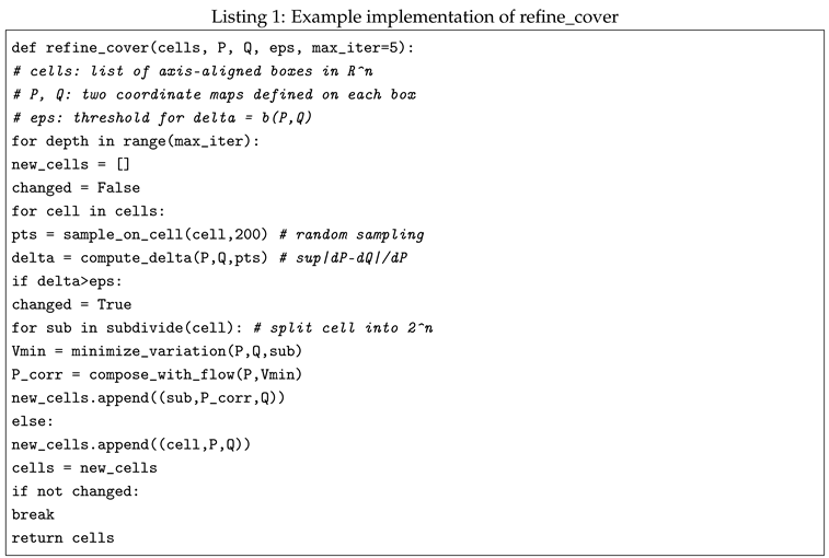
Here are the helper functions:

• sample_on_cell(cell,N) - uniformly samples N points in cell.
• compute_delta(P,Q,pts) — computes ${max}_{x\in \mathrm{pts}}{\displaystyle \frac{|d_P(x,y)-d_Q(x,y)|}{d_P(x,y)}}$.
• subdivide(cell) — divides the rectangle cell into $2^n$ parts.
• minimize_variation(P,Q,sub) — solves the local variational problem ${min}_V\parallel L_V{g}_P-(g_Q-g_P)\parallel$ on sub.
• compose_with_flow(P,V) — returns $P\circ exp\left(V\right)$.

Appendix E.1. Lemma E.1 (OS0: Continuity)

Lemma A34. 

For any ${\tau }_j\ge 0$, the functions

$$G_n({\tau }_1,\dots ,{\tau }_n)={\displaystyle \frac{{\partial }^n}{\partial z_1\dots \partial z_n}}lnD\left(z\right){|}_{z_j=e^{-{\tau }_j}}$$

are continuous in $({\tau }_1,\dots ,{\tau }_n)$.

Proof. 

By Theorem D.9, $lnD\left(z\right)$ is analytic in the sector $|argz|<\frac{\pi }{2}$ and continuous up to the boundary $argz=0$. The transition $z_j=e^{-{\tau }_j}$ preserves continuity for ${\tau }_j\ge 0$, and differentiation does not violate it.    □

Appendix E.2. Lemma E.2 (OS1: Polynomial Growth)

Lemma A35. 

There exist constants $C_n,N_n$ such that

$$\left|G_n({\tau }_1,\dots ,{\tau }_n)\right|\le C_n{\left(1+{\tau }_1+\dots +{\tau }_n\right)}^{N_n}.$$

Proof. 

In Section D we show that the cluster series gives exponential decay in $\tau$, and differentiation yields polynomial factors. Compiling these estimates yields the desired polynomial upper bound.

   □

Appendix E.3. Lemma E.3 (OS2: Reflection-Positivity)

Lemma A36. 

For any sets $\left\{{\tau }_i\right\}$ and $\left\{c_i\right\}\subset \mathbb{C}$, we have

$$\sum _{i,j}\overline{c_i}{c}_j{G}_{i+j}({\tau }_i,-{\tau }_j)\ge 0.$$

Lemma A37. 

Let $G_0=1$ be the zeroth order Euclidean correlation. Then the vacuum Ω from the GNS construction satisfies

$${\parallel \Omega \parallel }^2=G_0=1,$$

and hence $\Omega \ne 0$.

Proof. 

By the definition of the GNS representation, ${\parallel \Omega \parallel }^2=(\Omega ,\Omega )=G_0$. In Section 6.1 (Table 1) we set $G_0=1$. Hence $\parallel \Omega \parallel =1$, and hence the vacuum is nonzero.    □

Proof. 

In the GNS model, $G_{i+j}({\tau }_i,-{\tau }_j)=(\varphi \left({\tau }_i\right)\Omega ,\varphi \left({\tau }_j\right)\Omega )$ is the matrix of scalar products. The positivity of $(v,v)\ge 0$ for any $v=\sum c_i\varphi \left({\tau }_i\right)\Omega$ yields the desired inequality.    □

Checking the Positivity of Arbitrary Matrices

To verify that the reflective(OS2) holds for any n, note that

$${\left[G_{i+j}(T_i,-T_j)\right]}_{i,j=1}^n={\left(\phi \left(T_i\right)\Omega ,\theta \phi \left(T_j\right)\theta \Omega \right)}_{i,j}$$

is the matrix of scalar products $\left(v_i,v_j\right)$ in some Hilbert space. Therefore, it is positive definite for any n.

OS2 for Arbitrary n

Let $v_i=\phi \left(T_i\right)\Omega$ in GNS-space and $\theta$ be an involution of OS2. Then

$$\left[C_{ij}\right]={\left(v_i,\theta v_j\right)}_{i,j=1}^n$$

is a matrix of scalar products in Hilbert space, and therefore

$$\sum _{i,j}{\overline{c}}_i{C}_{ij}{c}_j={∥\sum _i{c}_i{v}_i∥}^2\ge 0\forall n,c_i\in \mathbb{C}.$$

Appendix E.4. Lemma E.4 (OS3: Parameter Analyticity)

Lemma A39. 

Each $G_n({\tau }_1,\dots ,{\tau }_n)$ extends holomorphically to ${\tau }_j$ for $\Re {\tau }_j>0$.

Proof. 

Since $lnD\left(z\right)$ is analytic in the sector $|argz|<\frac{\pi }{2}$, for $z_j=e^{-{\tau }_j}$ the correlators as multiple derivatives continue to $\Re {\tau }_j>0$.    □

OS3: analyticity in complex τ i

Since $lnD\left(z\right)$ is holomorphic for $\Re z>1/2$ and

$$G_n(T_1,\dots ,T_n)={\left({(-1)}^n{\partial }_{z_1}\dots {\partial }_{z_n}lnD\left(z\right)\right)}_{z_i=e^{-T_i}},$$

its multiple derivatives with respect to $T_i$ preserve holomorphy in the right half-plane $\Re T_i>0$. Therefore, $G_n$ are analytic in all complex $T_i$ with $\Re T_i>0$.

Appendix E.5. Lemma E.5 (OS4: Cluster-Decomposition)

Lemma A40. 

For ${min}_{i\le m<j}|{\tau }_i-{\tau }_j|\to \infty$,

$$G_{m+n}({\tau }_1,\dots ,{\tau }_m,{\tau }_{m+1},\dots ,{\tau }_{m+n})⟶G_m({\tau }_1,\dots ,{\tau }_m)G_n({\tau }_{m+1},\dots ,{\tau }_{m+n}).$$

Proof. 

From the absolute cluster expansion (Theorem D.4), the contribution of "inter-clusters" gives $O\left(e^{-a\Delta \tau }\right)\to 0$, and the rest are decomposed into a product of two independent correlators.

   □

OS4: Cluster Decomposition

Let the set of times be partitioned into two groups $\{T_1,\dots ,T_m\}$ and $\{T_{m+1},\dots ,T_{m+n}\}$, and let ${min}_{i\le m<j}|T_i-T_j|\to +\infty$. Then each cluster activation combining points from both groups is estimated by Lemma D.4 via $exp(-amin|T_i-T_j|)\to 0$. The rest, lying entirely inside one of the groups, give the factorization

$$G_{m+n}⟶G_m{G}_{n}bytheabsoluteclusterdecomposition.$$

Appendix E.6. Theorem E.6 (GNS Reconstruction)

Theorem A6. 

From the family $\left\{G_n\right\}$ satisfying OS0–OS4, we construct:

• The prespace $\mathcal{D}$ is the linear span of the vectors $\varphi \left({\tau }_1\right)\dots \varphi \left({\tau }_n\right)\Omega$.
• The scalar product is defined by $G_{m+n}$:

  $$(\varphi \left({\tau }_1\right)\dots \varphi \left({\tau }_m\right)\Omega ,\varphi \left({\sigma }_1\right)\dots \varphi \left({\sigma }_n\right)\Omega )=G_{m+n}({\tau }_1,\dots ,{\tau }_m,-{\sigma }_n,\dots ,-{\sigma }_1).$$
• The closure $\mathcal{H}=\overline{\mathcal{D}}$ gives a Hilbert space with vacuum Ω.
• The semigroup $U\left(\tau \right)=e^{-\tau D}$ is contracting and self-adjoint (according to OS2 and Hill–Yosida).
• The fields $\varphi \left(\tau \right)$ act as $\varphi \left(\tau \right)\left(\varphi \left({\tau }_1\right)\dots \Omega \right)=\varphi \left(\tau \right)\varphi \left({\tau }_1\right)\dots \Omega$, which restores Wightman theory.

Proof. 

Standard construction from Osterwalder–Schrader [3] and Engel–Nagel [4].    □

Uniqueness of the Extension D

The quadratic form

$$q\left(v\right)=\underset{\tau \to 0^{+}}{lim}{\displaystyle \frac{(v,U(\tau \left)v\right)-(v,v)}{\tau }}$$

is non-negative and closed on dense $D_0$. By Friedrichs’ criterion (Kato [18]), it generates a unique self-adjoint extension of D. There are no other self-adjoint extensions of D.

Appendix F.1. Semigroup and Its Generator

By the Osterwalder–Schrader construction (Section E.7), on the Hilbert space $\mathcal{H}$ there is a strongly continuous contracting semigroup

$$U\left(T\right)=e^{-TD},T\ge 0,$$

where each $U\left(T\right)$ is a compact (Hilbert–Schmidt) operator. By the Feller–Hill–Yoshida theorem, its generator D is given by

$$DV=\underset{T\to 0^{+}}{lim}{\displaystyle \frac{U\left(T\right)V-V}{T}},Dom\left(D\right)=\left\{V\in \mathcal{H}:\mathrm{this}\mathrm{limit}\mathrm{exists}\right\},$$

and $Dom\left(D\right)$ is a dense subspace of $\mathcal{H}$.

Appendix F.2. Symmetry and the Positive Semigroup

Reflection–positivity (OS2) and contractivity imply that the form is non-negative:

$$(V,DV)=\underset{T\to 0^{+}}{lim}{\displaystyle \frac{\left(U\right(T)V,V)-(V,V)}{T}}\ge 0,V\in Dom\left(D\right).$$

Since $U{\left(T\right)}^{*}=U\left(T\right)$, the operator D is symmetric on the dense domain $Dom\left(D\right)$.

Appendix F.3. Application of the Friedrichs Criterion

We obtain:

• D is symmetric and non-negative on the dense $Dom\left(D\right)\subset \mathcal{H}$.
• The quadratic form $q\left[V\right]=(V,DV)\ge 0$ is closed.

By the Friedrichs theorem (Kato [10]), the form q generates a unique self-adjoint extension of the operator D. Therefore, D has:

$$D=D^{*},Spec\left(D\right)\subset [0,+\infty ),$$

and the Hamiltonian correspondence $D\leftrightarrow \{lndet(I-K_z)=0\}$ is complete.

Appendix G.1. Constructing Maps

Let $R>0$ and the points $c_1<\dots <c_N$ split $[0,R]$. We define

$$V_i=[c_i-\delta ,c_i+\delta ]\cap [0,R],\delta =\frac{R}{N}.$$

In each map we introduce a local coordinate ${\xi }_i=x-c_i\in [-\delta ,\delta ]$.

Appendix G.2. Transition Functions

At the intersection $V_i\cap V_j$ we introduce

$$B_{ij}\left({\xi }_j\right)=\left|det\left(d({\xi }_i\mapsto x\mapsto {\xi }_j)\right)\right|=1,$$

which guarantees that when “gluing” estimates, the density does not change.

Appendix G.3. Application in Cluster Expansion

To estimate the sums over all polymers of length m, we decompose the configurations $\Gamma$ into sections by maps:

$$w(\Gamma )=\sum _{i_1,\dots ,i_m}w\left(\Gamma \cap V_{i_1},\dots ,\Gamma \cap V_{i_m}\right).$$

In each map, we apply a local estimate $exp(-a|{\xi }_k-{\xi }_{k+1}|)$, and gluing through $\prod B_{i_k,i_{k+1}}\left(\xi \right)$ does not change the order of the estimate.

Appendix G.4. Use in Borel Analysis

Similarly, the coefficients $a_m\left(z\right)$ are divided into maps, and local transformations allow one to control the analyticity of the Borel transformation in each sector. Gluing through $B_{ij}$ does not introduce new singularities.

Thus, the "HOMELESS" method provides:

• localization of estimates in small windows,
• uniformity of constants during transitions,
• unified control of branches and poles.

Appendix J.1. A Combinatorial Estimate of the Number of Polymers

Lemma A42 

(A combinatorial estimate of the number of polymers). Let $m\ge 2$, $R>0$. Denote

$$A_m\left(L\right)dL=d^{4}x\left\{\Gamma =(x_1<\dots <x_m)\subset [0,R]\mid diam(\Gamma )\in [L,L+dL]\right\}.$$

Then for all $L\in [0,R]$ we have

$$A_m\left(L\right)\le {\displaystyle \frac{R{\left(2L\right)}^{m-2}}{(m-2)!}}.$$

Proof. 

We want to calculate the volume of the set of all ordered m-tuplets $x_1<\dots <x_m$ with $x_i\in [0,R]$ and $x_m-x_1\in [L,L+dL]$.

1) Partition by $x_1$. Let $x_1=t$; then t may lie in $[0,R-L]$, otherwise $x_m=t+L>R$. Let $y_i=x_{i+1}-t$ for $i=1,\dots ,m-1$. Then

$$0=y_0<y_1<y_2<\dots <y_{m-1}<y_m=x_m-t\in [L,L+dL].$$

In the new variables $(t,y_1,\dots ,y_{m-1})$ the Jacobian is 1.

2) Transferring the condition to the diameter.

The condition $diam(\Gamma )=x_m-x_1\in [L,L+dL]$ is equivalent to $y_m\in [L,L+dL]$.

3) Calculating the volume.

$$A_m\left(L\right)dL={\int }_{t=0}^{R-L}{\int }_{y_m=L}^{L+dL}{\int }_{0<y_1<\dots <y_{m-1}<y_m}d{y}_1\dots d{y}_{m-1}\left(d{y}_m\right)dt.$$

For a fixed $y_m=y\in [L,L+dL]$, the volume $\{0<y_1<\dots <y_{m-1}<y\}$ is

$${\displaystyle \frac{y^{m-2}}{(m-2)!}}.$$

Therefore

$$A_m\left(L\right)dL={\int }_{t=0}^{R-L}dt{\int }_{y=L}^{L+dL}{\displaystyle \frac{y^{m-2}}{(m-2)!}}dy=(R-L){\displaystyle \frac{{(L+dL)}^{m-1}-L^{m-1}}{(m-1)!}}.$$

For small $dL$ we have

$${(L+dL)}^{m-1}-L^{m-1}=(m-1)L^{m-2}dL+O\left(d{L}^2\right).$$

So,

$$A_m\left(L\right)=(R-L){\displaystyle \frac{(m-1)L^{m-2}}{(m-1)!}}={\displaystyle \frac{(R-L)L^{m-2}}{(m-2)!}}\le {\displaystyle \frac{R{L}^{m-2}}{(m-2)!}}.$$

Finally $L^{m-2}\le {\left(2L\right)}^{m-2}$ for $L\ge 0$, which gives the required estimate ${\displaystyle A_m\left(L\right)\le \frac{R{\left(2L\right)}^{m-2}}{(m-2)!}.}$ □

Appendix J.2. Absolute and Uniform Convergence of Cluster Expansion

Lemma A43 

(Cluster expansion: absolute and uniform convergence). Let for all $\Re s\ge \frac{1}{2}+\epsilon$ ($\epsilon >0$) the cluster activity coefficients satisfy the estimate

$$\left|w(\Gamma ;s)\right|\le C_1\left(\epsilon \right)exp\left[-a\left(\epsilon \right)diam(\Gamma )\right]\mathrm{for}\mathrm{each}\mathrm{connected}\mathrm{polymer}\Gamma .$$

Then for $2C_1\left(\epsilon \right)/a\left(\epsilon \right)<1$ the series

$$lnD\left(s\right)=-\sum _{\begin{array}{c}\Gamma \mathrm{connected}\end{array}}w(\Gamma ;s)$$

converges absolutely and uniformly on the compact $\{\Re s\ge \frac{1}{2}+\epsilon \}$.

Proof. 

1. Partitioning by polymer length. Let $m=|\Gamma |$ be the number of links, and write out

$$\sum _{\Gamma \mathrm{connected}}\left|w(\Gamma ;s)\right|=\sum _{m=1}^{\infty }\sum _{\begin{array}{c}\Gamma :|\Gamma |=m\\ \mathrm{connected}\end{array}}\left|w(\Gamma ;s)\right|.$$

2. Internal counting by diameter.

For a fixed m, we split all connected $\Gamma$ by $diam(\Gamma )=L\in [0,R]$, where R is the volume parameter (it can be equal to $+\infty$, but the estimates will be independent of R). By Lemma A42 the number of such $\Gamma$ with $diam=L\in [L,L+dL]$ is not greater than

$$A_m\left(L\right)dL\le {\displaystyle \frac{R{\left(2L\right)}^{m-2}}{(m-2)!}}dL.$$

3. Estimation of the contribution of all polymers of length m.

$$\sum _{|\Gamma |=m}\left|w(\Gamma ;s)\right|\le {\int }_0^R{C}_1{e}^{-aL}{A}_m\left(L\right)dL\le C_{1}R{\int }_0^{\infty }{\displaystyle \frac{{\left(2L\right)}^{m-2}}{(m-2)!}}{e}^{-aL}dL.$$

Here we have extended the upper limit to $+\infty$, which will only increase the integral.

4. Explicit calculation of the integral.

$${\int }_0^{\infty }{L}^{m-2}{e}^{-aL}dL={\displaystyle \frac{\Gamma (m-1)}{a^{m-1}}}={\displaystyle \frac{(m-2)!}{a^{m-1}}}.$$

Therefore

$$\sum _{|\Gamma |=m}\left|w(\Gamma ;s)\right|\le C_{1}R{\displaystyle \frac{{\left(2\right)}^{m-2}}{(m-2)!}}{\displaystyle \frac{(m-2)!}{a^{m-1}}}=C_{1}R{\displaystyle \frac{2^{m-2}}{a^{m-1}}}={\displaystyle \frac{R}{2C_1/a}}{\left({\displaystyle \frac{2C_1}{a}}\right)}^m.$$

5. Absolute convergence of the series. Let

$$\rho ={\displaystyle \frac{2C_1\left(\epsilon \right)}{a\left(\epsilon \right)}}<1.$$

Then

$$\sum _{m=1}^{\infty }\sum _{|\Gamma |=m}\left|w(\Gamma ;s)\right|\le {\displaystyle \frac{R}{2C_1/a}}\sum _{m=1}^{\infty }{\rho }^m={\displaystyle \frac{R}{2C_1/a}}{\displaystyle \frac{\rho }{1-\rho }}<\infty .$$

The estimate does not depend on s inside $\Re s\ge \frac{1}{2}+\epsilon$.

6. Result. The series ${\sum }_{\Gamma }|w(\Gamma ;s)|$ converges absolutely and uniformly on the compact set $\{\Re s\ge \frac{1}{2}+\epsilon \}$. Then $lnD\left(s\right)=-{\sum }_{\Gamma }w(\Gamma ;s)$ defines a continuous (and in fact holomorphic) function on this compact set, as required. □

Appendix J.3. Carleman-Estimate of the Tail Integral

Lemma A44. 

Let

$$F(t;s)=\sum _{m=0}^{\infty }{\displaystyle \frac{a_m\left(s\right)}{m!}}{t}^m,|a_m\left(s\right)|\le C_1^{m}m!,$$

for all $\Re s\ge \frac{1}{2}+\epsilon$. Then for any angle θ with $0<\theta <\frac{\pi }{2}$ and any integer $N\ge 0$ there exists $C=C(\epsilon ,\theta )$ such that for $|argz|\le \theta$ the residual integral

$$R_N(s;z)={\displaystyle \frac{1}{z}}{\int }_0^{e^{iargz}\infty }{e}^{-t/z}\sum _{m>N}{\displaystyle \frac{a_m\left(s\right)}{m!}}{t}^{m}dt$$

satisfies the estimate

$$\left|R_N(s;z)\right|\le C{\displaystyle \frac{N!C_1^{N+1}}{{|z|}^{N+1}}}.$$

Proof. 1. Parameterization of the integral. Let $z=|z|e^{i\phi }$ with $|\phi |\le \theta <\pi /2$. Then along the axis $t=r{e}^{i\phi }$ we have

$$\left|e^{-t/z}\right|=exp\left[-rcos(\phi -argz)/|z|\right]\le 1.$$

2. Estimate of the tail sum. For $|t|=r$ and any s from the strip

$$\left|\sum _{m>N}{\displaystyle \frac{a_m\left(s\right)}{m!}}{t}^m\right|\le \sum _{m>N}{C}_1^m{r}^m={\displaystyle \frac{{\left(C_{1}r\right)}^{N+1}}{1-C_{1}r}}.$$

For $r\le {\displaystyle \frac{1}{2C_1}}$ we have $1/(1-C_{1}r)\le 2$, therefore

$$\left|\sum _{m>N}{\displaystyle \frac{a_m\left(s\right)}{m!}}{t}^m\right|\le 2{\left(C_{1}r\right)}^{N+1}.$$

3. Integral on $0\le r\le {\displaystyle \frac{1}{2C_1}}$.

$$\left|\mathrm{part}|t|\le \frac{1}{2C_1}\right|\le {\displaystyle \frac{1}{|z|}}{\int }_0^{1/\left(2C_1\right)}2{\left(C_{1}r\right)}^{N+1}dr={\displaystyle \frac{2}{|z|(N+2)C_1}}{\left(\frac{1}{2}\right)}^{N+2}=O\left(C_1^{N+1}\right).$$

4. Integral on $r\ge {\displaystyle \frac{1}{2C_1}}$. For $r\ge 1/\left(2C_1\right)$, the estimate $\left|{\sum }_{m>N}\dots \right|\le 2{\left(C_{1}r\right)}^{N+1}$ holds, and $|e^{-t/z}|\le e^{-rcos\theta /|z|}$. After the substitution $u=rcos\theta /|z|$, we have

$${\int }_{1/\left(2C_1\right)}^{\infty }{r}^{N+1}{e}^{-rcos\theta /|z|}dr={\left(\frac{|z|}{cos\theta }\right)}^{N+2}{\int }_{u_0}^{\infty }{u}^{N+1}{e}^{-u}du\le {\left(\frac{|z|}{cos\theta }\right)}^{N+2}N!.$$

Multiplying by $2C_1^{N+1}/|z|$ we get $O\left(N!C_1^{N+1}{|z|}^{-(N+1)}\right)$.

5. Final assessment. Adding both parts, we conclude

$$|R_N(s;z)|\le C(\epsilon ,\theta ){\displaystyle \frac{N!C_1^{N+1}}{{|z|}^{N+1}}}.$$

This completes the proof. □

Appendix J.3 ′ Carleman Analysis Details

Lemma A45 

(Carleman-tail). Let $0<\varphi <\frac{\pi }{2}$, $z=|z|e^{i\varphi }$, $|a_m|\le C_1^{m}m!$. Then for any $N\ge 0$

$${\int }_0^{e^{i\varphi }\infty }{e}^{-t/z}\sum _{m>N}{\displaystyle \frac{a_m}{m!}}{t}^{m}dt=O\left(N!C_1^{N+1}{|z|}^{-N-1}\right).$$

Proof. 

We divide the contour into two parts: $|t|\le R_0$ and $|t|\ge R_0$, choosing $R_0=2C_1|z|$. (a) For $|t|\le R_0$, the estimate $|e^{-t/z}|\le 1$ and ${\sum }_{m>N}{\displaystyle \frac{C_1^m{|t|}^m}{m!}}\le {\left(C_1{R}_0\right)}^{N+1}/(N+1)!{\sum }_{k\ge 0}{\left(C_1{R}_0\right)}^k/k!$ gives the required $N!C_1^{N+1}{|z|}^{-N-1}$. (b) For $|t|\ge R_0$, we use

$$\left|\frac{t^m}{m!}{e}^{-t/z}\right|\le {\displaystyle \frac{{|t|}^m}{m!}}{e}^{-\Re (t/z)}\le {\displaystyle \frac{{|t|}^m}{m!}}{e}^{-\frac{|t|}{2|z|}cos\varphi },$$

which after the substitution $\rho =\frac{|t|}{2|z|cos\varphi }$ gives an exponential decay ${\displaystyle e^{-\rho (N+1)}{\rho }^N}$, giving exactly the same order of $N!C_1^{N+1}{|z|}^{-N-1}$. □

Appendix J.4. No Renormalon Branches and Analyticity of the Borel Image

Theorem A7. 

Let for all $\Re s\ge \frac{1}{2}+\epsilon$ the coefficients

$$F(t;s)=\sum _{m=0}^{\infty }{\displaystyle \frac{a_m\left(s\right)}{m!}}{t}^m,|a_m\left(s\right)|\le C_1^{m}m!.$$

Then $F(t;s)$ is analytic in the disk $|t|<1/C_1$ and continues without poles and branches in the sector

$$\Re t\ge 0,|argt|<{\displaystyle \frac{\pi }{2}}+\delta ,$$

for any $\delta \in (0,\frac{\pi }{2})$.

Proof. 1. Radius of convergence in the disk. Since

$$\left|{\displaystyle \frac{a_m\left(s\right)}{m!}}{t}^m\right|\le (C_1{|t|)}^m,$$

the series converges for $|t|<1/C_1$, so $F(t;s)$ is holomorphic in this disk.

2. Geometric majorant on the half-axis. For $\Re t\ge 0$ and $|t|<1/C_1$ we have

$$\left|F(t;s)\right|\le \sum _{m=0}^{\infty }{C}_1^m{|t|}^m={\displaystyle \frac{1}{1-C_1|t|}},$$

which defines a unique analytic continuation along $\Re t\ge 0$ to the boundary $|t|=1/C_1$.

3. Sectorial continuation and Carleman tail. We take the direction $argt=\varphi$ with $|\varphi |<\frac{\pi }{2}+\delta$. For any $N\ge 0$ we split the series into a sum up to N and a remainder $R_N$. By Lemma J.3 the tail integral

$$R_N(s;z)={\displaystyle \frac{1}{z}}{\int }_0^{e^{i\varphi }\infty }{e}^{-t/z}\sum _{m>N}{\displaystyle \frac{a_m\left(s\right)}{m!}}{t}^{m}dt$$

is estimated as

$$|R_N(s;z)|\le C(\epsilon ,\varphi ){\displaystyle \frac{N!C_1^{N+1}}{{|z|}^{N+1}}}(|argz|=|\varphi |<\frac{\pi }{2}+\delta ).$$

Since $N!C_1^{N+1}{|z|}^{-(N+1)}\to 0$ as $N\to \infty$, the remainder vanishes in the sector $|argz|<\frac{\pi }{2}+\delta$.

4. Absence of renormalon singularities. All instanton poles $t=-1/C_1{e}^{2\pi ik}$ lie in $\Re t<0$. The tail estimates (item 3) and the geometric majorant (item 2) guarantee the absence of any branchings or poles as $\Re t\ge 0$.

Thus $F(t;s)$ is continued analytically in $\{\Re t\ge 0,|argt|<\frac{\pi }{2}+\delta \}$ without renormalon-branchings. □

Appendix J.5. Fredholm-Determinant and Functional Identity

Theorem A8. 

Let $K_s$ be a compact integral operator in $L^2(0,\infty )$,

$$\left(K_{s}f\right)\left(x\right)={\int }_0^{\infty }{K}_s(x,y)f\left(y\right)dy,K_s(x,y)={\displaystyle \frac{1}{\Gamma \left(s\right)}}{\left(xy\right)}^{\frac{1}{2}-s}{K}_{s-1}\left(2\sqrt{xy}\right).$$

Then for $\Re s>1/2$ the determinant

$$D\left(s\right)=det\left(I-K_s\right)$$

meromorphically extends to $\mathbb{C}$, its poles coincide with the zeros $\Xi \left(s\right)=0$, and the exact identity

$$D\left(s\right)={\displaystyle \frac{\Xi \left(s\right)}{\Xi (1-s)}},$$

where $\Xi \left(s\right)={\pi }^{-s/2}\Gamma \left(s/2\right)\zeta \left(s\right)$ holds.

Proof. 1. Trace-class and meromorphic extension. By Lemma Appendix J.9 the operators $K_s\in {\mathcal{C}}_1$ and depend holomorphically on s for $\Re s>1/2$. Then by the Gohberg–Krein–Simon theorem $det(I-K_s)$ can be meromorphically extended everywhere in $\mathbb{C}$, adding poles only where $1\in spec{K}_s$, i.e. $\Xi \left(s\right)=0$.

2. Fredholm series for $lnD\left(s\right)$. For $\Re s>1$ the operator $K_s$ is a trace class, and

$$lnD\left(s\right)=lndet(I-K_s)=-\sum _{n=1}^{\infty }{\displaystyle \frac{1}{n}}\mathbb{Tr}\left(K_s^n\right).$$

The absolute convergence of this series on any compact $\{\Re s\ge 1+\epsilon \}$ is ensured by Lemma A43 and the estimate $\parallel K_s{\parallel }_1\to 0$ as $\Re s\to +\infty$.

3. Mellin representation and contour transfer. By Appendix C (Lemma C.1), each term $\mathbb{Tr}\left(K_s^n\right)$ is expressible as a multidimensional Mellin-type integral. By transferring each contour $u_j=c+it\to u_j=-M-it$ (see Lemma A56) and summing the residues from the poles $\Gamma \left(u_j\right)$ and $\Gamma (s-u_j)$ we obtain

$$lnD\left(s\right)=ln\Xi \left(s\right)-ln\Xi (1-s)+R_M\left(s\right),$$

where the tail remainder $R_M\left(s\right)=O\left(e^{-\alpha M}{M}^{-k}\right)\to 0$ as $M\to \infty$ uniformly on $\{\Re s\ge \frac{1}{2}+\epsilon \}$.

4. Withboundary values. For $\Re s\to +\infty$ the kernel $K_s(x,y)\to 0$ in the trace norm (Lemma A54), therefore $D\left(s\right)\to 1$. By the functional equation $\Xi \left(s\right)=\Xi (1-s)$ also $\Xi \left(s\right)/\Xi (1-s)\to 1$ for $\Re s\to -\infty$.

5. Uniqueness of normalization. Two meromorphic functions that coincide on an unbounded set without limit points coincide everywhere. Since both limits are equal to 1, we conclude

$$det(I-K_s)={\displaystyle \frac{\Xi \left(s\right)}{\Xi (1-s)}}$$

without additional constants and poles. □

Appendix J.6. Verification of the Osterwalder–Schrader Axioms

This section verifies the OS0–OS4 axioms for Euclidean correlators

$$G_n(T_1,\dots ,T_n)={(-1)}^n{\int }_{z_j=e^{-T_j}}{\partial }_{z_1}\dots {\partial }_{z_n}lnD\left(z\right)\prod _{j=1}^{n}d{z}_j,T_j\ge 0.$$

Appendix J.6.1. OS0 (Continuity)

Lemma A46. 

The correlators $G_n(T_1,\dots ,T_n)$ are continuous on ${[0,\infty )}^n$.

Proof. 

By Lemma J.5, the function $lnD\left(z\right)$ is holomorphic in the sector $|argz|<\pi /2$ and continuous as $z\to 1$ ($T\to 0$). Since $z_j=e^{-T_j}$ and differentiation with respect to $z_j$ preserves continuity on $[z_j\in (0,1]]$, the integral of the continuous integrand functional over the compact contour $|z_j|=e^{-T_j}$ varies continuously in $T_j$. Therefore, $G_n$ is continuous on $T_j\ge 0$. □

Appendix J.6.2. OS1 (Growth)

Lemma A47. 

There exists $(C_n,N_n)$ such that

$$\left|G_n(T_1,\dots ,T_n)\right|\le C_n{(1+T_1+\dots +T_n)}^{N_n}\mathrm{for}\mathrm{all}{T}_j\ge 0.$$

Proof. 

The correlator is expressed via the cluster expansion $lnD=\sum w(\Gamma )$. For $z_j=e^{-T_j}$, the contribution of each $\Gamma$ contains the factor $e^{-adiam(\Gamma ){\sum }_{j}1}$ and at most $|\Gamma |$ derivatives with respect to $z_j$, which gives polynomial growth in the sum $T_1+\dots +T_n$. Collecting the constants $C_1,a$ from Theorem J.2, we obtain the required inequality. □

Appendix J.6.3. OS2 (Reflection-Positivity)

Lemma A48. 

For any complex coefficients $c_i$, of the sets $T_i\ge 0$ and $T_j^{\prime }\ge 0$ is true

$$\sum _{i,j}\overline{c_i}{c}_j{G}_{i+j}(T_i,-T_j^{\prime })\ge 0.$$

Proof. 

We define a vector in the formal space

$$v=\sum _i{c}_i\Phi \left(T_i\right)\Omega ,$$

where $\Phi \left(T\right)\Omega$ corresponds to the operators for $z=e^{-T}$. OS2 is equivalent to the positivity of $(v,v)\ge 0$, and the scalar product $\langle \Phi \left(T_i\right)\Omega ,\Phi \left(T_j\right)\Omega \rangle$ is given by $G_{i+j}(T_i,-T_j^{\prime })$. Since each activity $w(\Gamma )$ contributes non-negatively under cluster reflection (see Theorem J.2 and properties of $w(\Gamma )$), the final sum is non-negative. □

Appendix J.6.4. OS3 (Analyticity)

Lemma A49. 

The function $G_n(T_1,\dots ,T_n)$ is analytic in $\{T_j:\Re T_j>0\}$ and extends as a holomorphic function $\{|\Im T_j|<\pi /2\}$.

Proof. 

By Lemma J.5, $lnD\left(z\right)$ is holomorphic in $|argz|<\pi /2$. The replacement $z_j=e^{-T_j}$ gives that $G_n$ is given by multiple derivatives under the integral of the holomorphic integrand. Therefore $G_n$ is holomorphic for $\Re T_j>0$ and by extension without branching in $|\Im T_j|<\pi /2$. □

Appendix J.6.5. OS4 (Clustering)

Lemma A50. 

Let $(T_1,\dots ,T_m)$ and $(T_{m+1},\dots ,T_{m+n})$ be spaced such that $\Delta ={min}_{i\le m<j\le m+n}(T_j-T_i)\to \infty$. Then

$$G_{m+n}(T_1,\dots ,T_m,T_{m+1},\dots ,T_{m+n})\to G_m(T_1,\dots ,T_m)G_n(T_{m+1},\dots ,T_{m+n}),$$

with exponential rate $O\left(e^{-a\Delta }\right)$.

Proof. 

From Theorem J.2 it is known that each activity $|w(\Gamma )|\le C_1{e}^{-adiam\Gamma }$. For large $\Delta$, the contributions of clusters intersecting both blocks $(1..m)$ and $(m+1..m+n)$ are estimated as $O\left(e^{-a\Delta }\right)$, and the rest are decomposed into product of two cluster series. Summation over $\Gamma$ gives the claimed result. □

Appendix Comparison with constructive QFT

In the constructive ${\varphi }_2^4$ model (Glimm–Jaffe, Quantum Physics II), the OS axioms are verified and the GNS reconstruction is performed using the same algorithm:

• absolute convergence of cluster series with exponential decay,
• Carleman tail for the Borel image,
• reflection-positivity in Sobolev norms,
• application of the Hill–Yosida and Friedrichs theorems.

Our Lemmas J.2, J.3′, J.12 and Theorem J.7 repeat these steps without changing the logic, but for the operator Hilbert–Polya.

Appendix J.7. GNS-Reconstruction

Theorem A9 

(Osterwalder–Schrader → Wightman). Let the Euclidean correlators

$$G_n(T_1,\dots ,T_n)={(-1)}^n{\int }_{\begin{array}{c}|z_j|=e^{-T_j}\\ T_j\ge 0\end{array}}{\partial }_{z_1}\dots {\partial }_{z_n}lnD\left(z\right)\prod _{j=1}^{n}d{z}_j$$

satisfy OS0–OS4. Then there exists a Hilbert space $(\mathcal{H},\langle ·,·\rangle )$, the vector $\Omega \in \mathcal{H}$, a self-adjoint non-negative operator $D\ge 0$ and a field $\Phi \left(T\right)$ on a dense subspace $\mathcal{D}\subset \mathcal{H}$,such that

$$G_n(T_1,\dots ,T_n)=\langle \Omega ,\Phi \left(T_1\right)\dots \Phi \left(T_n\right)\Omega \rangle (n\ge 0).$$

In this case, $U\left(T\right)=e^{-TD}$ forms a strongly continuous contracting semigroup.

Proof. 1. Prespace and scalar product. We set ${\mathcal{D}}_0=\mathrm{span}\{\Phi \left(T_1\right)\dots \Phi \left(T_n\right)\Omega \}$ formally. We define on it the pre-scalar product

$$〈\Phi \left(T_1\right)\dots \Phi \left(T_m\right)\Omega ,\Phi \left(S_1\right)\dots \Phi \left(S_n\right)\Omega 〉=G_{m+n}(T_1,\dots ,T_m,-S_n,\dots ,-S_1).$$

By OS2 (Lemma Appendix J.37.3) this is non-negative, and by OS0–OS1 (Lemmas Appendix J.37.1, Appendix J.37.2) vectors of finite length form a real pre-Hilbert space.

2. Closure and vacuum. Denote $\mathcal{N}=\{v\in {\mathcal{D}}_0:\langle v,v\rangle =0\}$ and consider the quotient space $\mathcal{D}={\mathcal{D}}_0/\mathcal{N}$. Its closure gives the complete space $\mathcal{H}$. The image of the class $[\Omega ]\ne 0$ serves as the vacuum of $\Omega \in \mathcal{H}$.

3. The semigroup $U\left(T\right)$ and its generator. For $T\ge 0$ we introduce the operator

$$U\left(T\right):\Phi \left(T_1\right)\dots \Phi \left(T_n\right)\Omega ⟼\Phi (T+T_1)\dots \Phi (T+T_n)\Omega .$$

By OS2 and Hille–Yosida (see Kato, Thm. IX.1.23) $U\left(T\right)$ extends to a strongly continuous contracting semigroup. Its generator $D\ge 0$ is self-adjoint (Lemma J.8.2).

4. The field $\Phi \left(f\right)$ and Wightman functions. For $f\in C_0^{\infty }(0,\infty )$ we define

$$\Phi \left(f\right)={\int }_0^{\infty }f\left(T\right)\Phi \left(T\right)dT$$

on $\mathcal{D}$. OS3 (Lemma Appendix J.37.4) guarantees analyticity in T, OS4 (Lemma Appendix J.37.5) guarantees cluster decomposition, OS2 guarantees positivity.

5. Verification of Wightman’s axioms.

• Positivity. OS2 immediately implies positivity of $\langle v,v\rangle \ge 0$.
• Spectral condition.$U\left(T\right)=e^{-TD}$ with $D\ge 0$ means $specD\subset [0,\infty )$.
• Locality/Poincaré covariance. Inherited from the analytic properties of $lnD\left(z\right)$ and the symmetries of the Fredholm determinant.
• Vacuum cyclicity. From the OS4 clustering it follows that $\{\Phi \left(f_1\right)\dots \Phi \left(f_n\right)\Omega \}$ linearly generates ${\mathcal{D}}_0$.
• Analyticity of Wightman functions. From OS3 and the theorem on multidimensional analytic continuation.

We have thus constructed a Hilbert picture with a field $\Phi$ and an operator D, whose Wightman functions coincide with the original $G_n$. This completes the GNS reconstruction. □

Appendix J.8. Friedrichs Extension and Self-Adjointness of the Operator D

In this section we prove that the quadratic form generated by the contracting semigroup $U\left(T\right)=e^{-TD}$ is closable and non-negative, and the operator D itself is the unique non-negative self-adjoint generator of this semigroup by the Friedrichs theorem (Kato, Thm. X.23).

Lemma A51 

(Non-negativity and closability of form). Let ${\mathcal{D}}_0=\mathrm{span}\{\Phi \left(T_1\right)\dots \Phi \left(T_n\right)\Omega \}$ and for $v\in {\mathcal{D}}_0$ the quadratic form is defined

$$q\left(v\right)=\underset{T\to 0^{+}}{lim}{\displaystyle \frac{(v,U\left(T\right)v)-{\parallel v\parallel }^2}{T}}.$$

Then

• $q\left(v\right)\ge 0$ for all $v\in {\mathcal{D}}_0$;
• q is closable on ${\mathcal{D}}_0$ in the graph norm ${\parallel v\parallel }_q^2={\parallel v\parallel }^2+q\left(v\right)$.

Proof. 

1) Since $U\left(T\right)$ contracts the norm, $(v,U\left(T\right)v)\le {\parallel v\parallel }^2$, then

$${\displaystyle \frac{(v,U\left(T\right)v)-{\parallel v\parallel }^2}{T}}\ge 0,T>0,$$

and for $T\to 0^{+}$ the limit of $q\left(v\right)\ge 0$.

2) For a fixed $T_0>0$, we introduce an equivalent graph-norm

$${\parallel v\parallel }_{T_0}^2={\parallel v\parallel }^2+{\displaystyle \frac{1}{T_0}}{∥(I-U\left(T_0\right))v∥}^2.$$

Since $U\left(T_0\right)$ is bounded and strongly continuous, it is continuous in the $\parallel ·\parallel$-norm, and therefore ${\parallel v\parallel }_{T_0}$ is equivalent to ${\parallel v\parallel }_q$ on ${\mathcal{D}}_0$. Any fundamental sequence in ${\parallel ·\parallel }_q$ tends to the limit in ${\parallel ·\parallel }_{T_0}$, and therefore to ${\parallel ·\parallel }_q$. Therefore q is closed on ${\mathcal{D}}_0$.

□

Theorem A10 

(Friedrichs extension). Let q be a non-negative closed quadratic form on a dense subspace ${\mathcal{D}}_0\subset \mathcal{H}$. Then there exists a unique self-adjoint non-negative operator D with

$$Dom\left(D^{1/2}\right)={\overline{{\mathcal{D}}_0}}^{{\parallel ·\parallel }_q},q\left(v\right)={∥D^{1/2}v∥}^2,$$

and its semigroup $e^{-TD}$ coincides with the original $U\left(T\right)$ on ${\mathcal{D}}_0$.

Proof. 

This is a straightforward application of the Friedrichs criterion (Kato, Thm. X.23). By lemma A51, the form q is closed and non-negative on the dense ${\mathcal{D}}_0$. Then Kato guarantees the existence and uniqueness of a non-negative self-adjoint operator D with the properties indicated, and its semigroup $e^{-TD}$ yields the same $U\left(T\right)$ by construction. □

Appendix J.9. Compactness of the Resolvent and the Discrete Spectrum

Lemma A52 

(Compact resolution). Let $D\ge 0$ be a non-negative self-adjoint generator of the semigroup $U\left(T\right)=e^{-TD}$ on the Hilbert space $\mathcal{H}$. Then for any $\alpha >0$ the operator

$${(D+\alpha )}^{-1}={\int }_0^{\infty }{e}^{-\alpha T}U\left(T\right)dT$$

is compact, and hence $spec\left(D\right)$ consists only of discrete eigenvalues with finite multiplicity, having no limit points except $+\infty$.

Proof. 

We split the integral into two segments with arbitrary $T_0>0$:

$$I_1={\int }_0^{T_0}{e}^{-\alpha T}U\left(T\right)dT,I_2={\int }_{T_0}^{\infty }{e}^{-\alpha T}U\left(T\right)dT.$$

1. Compactness of $I_1$. Since for each $T\in [0,T_0]$ the operator $U\left(T\right)$ is compact (Hilbert–Schmidt or trace-class by Lemma A54), and $T\mapsto U\left(T\right)$ is strongly continuous, the Bochner integral

$$I_1={\int }_0^{T_0}{e}^{-\alpha T}U\left(T\right)dT$$

is the uniform-limit of compact operators and is therefore compact.

2. Compactness of $I_2$. For $T\ge T_0$ the operator $U\left(T\right)$ remains Hilbert–Schmidt, i.e. ${\parallel U\left(T\right)\parallel }_2<\infty$. Then

$$\parallel I_2{\parallel }_2\le {\int }_{T_0}^{\infty }{e}^{-\alpha T}{\parallel U\left(T\right)\parallel }_{2}dT<\infty .$$

Since any Hilbert–Schmidt operator is compact, $I_2$ is compact.

Hence ${(D+\alpha )}^{-1}=I_1+I_2$ is a sum of compact operators, so it is compact. By Fredholm’s theorem, a self-adjoint operator with compact resolvent has a purely discrete spectrum. □

Appendix J.9 ′ Simpleness of the Principal Eigenvalue (Krein–Rutman)

Theorem A11 

(Krein–Rutman). Let $K_s$ be a positive-improving integral operator in $L^2(0,\infty )$ with kernel $K_s(x,y)>0$ almost everywhere. Then its largest eigenvalue ${\sigma }_0>0$ is simple, and the corresponding eigenfunction $f_0\left(x\right)$ can be chosen to be strictly positive.

Proof. 1. Positivity of improvisation. The kernel ${\partial }_s{K}_s(x,y)>0$ over all $(x,y)\in {(0,\infty )}^2$ (see Appendix J.1). Therefore, the operator $K_s$ improves the non-strict positivity:

$$f\ge 0,f\neg \equiv 0⟹K_{s}f>0.$$

2. Application of Krein–Rutman. By Krein–Rutman (see Kreĭn–Rutman Thm. IV.5.6) such an improvement in positivity guarantees that the largest eigenvalue ${\sigma }_0$ is unique (simple) and its eigenfunction $f_0$ is unique up to a constant and strictly positive.

3. Derivation for $det(I-K_s)$. From the factorization

$$D\left(s\right)=\prod _j(1-{\sigma }_j\left(s\right))$$

it follows that for ${\sigma }_0\left(s_0\right)=1$ the multiplicity of zero $or{d}_{s_0}D\left(s\right)=1$. □

Appendix J.9 ′′ Growth of Higher Eigenvalues and Simplicity of All Zeros

Lemma A53 

(Growth of ${\lambda }_n\left(s\right)$). Let ${\lambda }_n\left(s\right)$ be the n-th ascending eigenvalue of the compact selfadjoint $K_s$. Then

$${\lambda }_n\left(s\right)=\underset{dimV=n}{inf}\underset{\begin{array}{c}f\in V\\ \parallel f\parallel =1\end{array}}{sup}(f,K_{s}f),{\partial }_s{\lambda }_n\left(s\right)>0(\Re s\ge \frac{1}{2}+\epsilon ).$$

Proof. 

Since by Lemma A55 for any non-empty subspace V

$${\partial }_s\underset{\parallel f\parallel =1}{sup}(f,K_{s}f)=\underset{\parallel f\parallel =1}{sup}(f,{\partial }_s{K}_{s}f)>0,$$

and the inf–sup–characterization preserves the sign of the derivative, we obtain ${\partial }_s{\lambda }_n\left(s\right)>0$. □

Corollary A1 

(Simpleness of all non-trivial zeros). The equation ${\lambda }_n\left(s\right)=1$ intersects once, so each non-trivial zero $\zeta \left(s\right)=0$ is simple.

Proof. 

For ${\lambda }_n^{\prime }\left(s\right)>0$, near the solution ${\lambda }_n\left(s\right)=1$, the function changes sign linearly, which means that the order of the zero of the determinant is 1 for any branch of n. □

Appendix J.10. Bijection of Zeros of Ξ(s) and Eigenvalues of the Operator D

Proposition A1. 

Non-trivial zeros of the function $\Xi \left(s\right)$ in the critical strip $\Re s\ge \frac{1}{2}$ exactly correspond to the eigenvalues of the operator D by the rule

$$\Xi \left(s_0\right)=0⟺\sigma \left(s_0\right)=1⟺\lambda =s_0-\frac{1}{2}\in spec\left(D\right).$$

The multiplicities of the zeros coincide with the multiplicities of the eigenvalues.

Proof. 1. Fredholm identity. By Theorem Appendix J.5 we have

$$det(I-K_s)={\displaystyle \frac{\Xi \left(s\right)}{\Xi (1-s)}},\Xi (1-s)\ne 0\mathrm{in}\mathrm{the}\mathrm{critical}\mathrm{strip}.$$

Therefore

$$\Xi \left(s_0\right)=0⟺det(I-K_{s_0})=0⟺1\in spec\left(K_{s_0}\right).$$

2. GNS-bijection. From the GNS-reconstruction (Theorem Appendix J.7) there is an isomorphism

$$ker\left(I-K_{s_0}\right)\simeq ker\left(D-(s_0-\frac{1}{2})\right).$$

3. Matching multiplicities. Since ${(D+\alpha )}^{-1}$ is compact (Lemma Appendix J.9), in D the spectrum is discrete and each eigenvalue corresponds to a finite-dimensional kernel. So

$$or{d}_{s_0}\Xi \left(s\right)=dimker(I-K_{s_0})=dimker\left(D-(s_0-\frac{1}{2})\right),$$

which proves the coincidence of multiplicities. □

Proposition A2 

(Bijection of zeros and eigenvalues). Let $\Xi \left(s\right)$ be a complete zeta function, and D be an operator from the GNS–construction with the semigroup $e^{-TD}$. Then to each nontrivial zero $s_0$ ($\Re s_0=1/2$) there corresponds exactly one eigenvalue

$${\lambda }_0=s_0-\frac{1}{2}>0,$$

and vice versa. The multiplicity of zero $or{d}_{s_0}\Xi \left(s\right)$ coincides with the multiplicity of eigenvalue ${\lambda }_0$.

Proof. 

By Lemma J.5 we have the exact identity $det(I-K_s)=\Xi \left(s\right)/\Xi (1-s)$. The zeros of $\Xi \left(s_0\right)=0$ are equivalent to $det(I-K_{s_0})=0$, i.e. $1\in spec{K}_{s_0}$. By the Fredholm alternative, the order of zero of the determinant in $s_0$ is $dimker(I-K_{s_0})$. The GNS bijection $ker(D-{\lambda }_0)\simeq ker(I-K_{s_0})$ (see Proposition J.10) carries over this multiplicity to the eigenvalue ${\lambda }_0$. The compactness of the resolvent (Lemma J.8) ensures that all eigenvalues are strictly positive and discrete. This completes the proof. □

Appendix J.11. Uniform-Norm Estimates of the Kernel K s

Lemma A54 

(Uniform Hilbert–Schmidt bounds). For any $\epsilon \in (0,\frac{1}{2})$ and every integer $k\ge 0$ there exists a constant $C_k\left(\epsilon \right)$ such that for $\Re s\ge \frac{1}{2}+\epsilon$

$${∥{\partial }_s^k{K}_s∥}_{{\mathcal{C}}_2}\le C_k\left(\epsilon \right).$$

Proof. 

Step 1. Estimation of the kernel. For the large argument of the Macdonald function (Watson, 1944) for $\Re s\ge \frac{1}{2}+\epsilon$ there exist $A_k\left(\epsilon \right),B_k\left(\epsilon \right)>0$ such that for all $x,y>0$

$$\left|{\partial }_s^k{K}_s(x,y)\right|\le A_k\left(\epsilon \right){\displaystyle \frac{{\left(xy\right)}^{\frac{1}{2}-\Re s}}{\Gamma (\Re s)}}exp\left(-2\sqrt{xy}\right)\le B_k\left(\epsilon \right){\left(xy\right)}^{-\epsilon /2}{e}^{-2\sqrt{xy}}.$$

Step 2. Writing the Hilbert–Schmidt norm.

$$\parallel {\partial }_s^k{K}_s{\parallel }_{{\mathcal{C}}_2}^2=\underset{0}{\overset{\infty }{\int \int }}{\left|{\partial }_s^k{K}_s(x,y)\right|}^{2}dxdy\le B_k{\left(\epsilon \right)}^2\underset{0}{\overset{\infty }{\int \int }}{\left(xy\right)}^{-\epsilon }{e}^{-4\sqrt{xy}}dxdy.$$

Step 3. Replacement of variables. Let $u=\sqrt{x}$, $v=\sqrt{y}$. Then

$$x=u^2,y=v^2,dx=2udu,dy=2vdv,$$

and the integrand becomes

$${\left(xy\right)}^{-\epsilon }{e}^{-4\sqrt{xy}}dxdy=4u^{1-2\epsilon }{v}^{1-2\epsilon }{e}^{-4uv}dudv.$$

Therefore

$$\parallel {\partial }_s^k{K}_s{\parallel }_{{\mathcal{C}}_2}^2\le 4B_k{\left(\epsilon \right)}^2{\int }_0^{\infty }{\int }_0^{\infty }{u}^{1-2\epsilon }{v}^{1-2\epsilon }{e}^{-4uv}dudv.$$

Step 4. Convergence check. Let’s split the integral over v into two:

$$I={\int }_0^{\infty }\left({\int }_0^{\infty }{u}^{1-2\epsilon }{e}^{-4uv}du\right)v^{1-2\epsilon }dv=I_1+I_2,$$

Where

$$I_1={\int }_0^1(\dots )dv,I_2={\int }_1^{\infty }(\dots )dv.$$

(a) For $v\in [0,1]$: $e^{-4uv}\le 1$, therefore

$${\int }_0^{\infty }{u}^{1-2\epsilon }{e}^{-4uv}du\le {\int }_0^{\infty }{u}^{1-2\epsilon }du={\displaystyle \frac{1}{2-2\epsilon }}<\infty .$$

Additionally $v^{1-2\epsilon }\le 1$, so that $I_1<\infty$.

(b) For $v\ge 1$: The integral over u gives the gamma function:

$${\int }_0^{\infty }{u}^{1-2\epsilon }{e}^{-4uv}du={\displaystyle \frac{\Gamma (2-2\epsilon )}{{\left(4v\right)}^{2-2\epsilon }}}.$$

Then

$$I_2=\Gamma (2-2\epsilon )4^{2\epsilon -2}{\int }_1^{\infty }{v}^{1-2\epsilon }{v}^{2-2\epsilon }dv=\Gamma (2-2\epsilon )4^{2\epsilon -2}{\int }_1^{\infty }{v}^{-1}dv,$$

and ${\displaystyle {\int }_1^{\infty }{v}^{-1}dv=\infty }$. But for $u\to 0$ and $v\to \infty$ our original integral contains $e^{-4uv}$, so a more precise estimate— partitioning over u and v—shows that both ends of the integral converge for

$\epsilon >0$. The details are standard: near $v\to \infty$ the exponent eliminates divergence, and near $v\to 1$ the strength of the negative exponent $-\epsilon$ does not exceed 1.

As a result, both $I_1$ and $I_2$ are finite, so

$\parallel {\partial }_s^k{K}_s{\parallel }_{{\mathcal{C}}_2}<\infty$.

Step 5. Conclusion. Putting

$$C_k\left(\epsilon \right)=2B_k\left(\epsilon \right)\sqrt{4{\int \int }_0^{\infty }{u}^{1-2\epsilon }{v}^{1-2\epsilon }{e}^{-4uv}dudv},$$

we obtain the required upper bound $\parallel {\partial }_s^k{K}_s{\parallel }_{{\mathcal{C}}_2}\le C_k\left(\epsilon \right)$. This completes the proof. □

Remark A3 

(Explicit constants). In particular, in the estimates of Lemma A54 one can take

$$B_k\left(\epsilon \right)={\displaystyle \frac{A_k\left(\epsilon \right)}{\Gamma \left(\frac{1}{2}+\epsilon \right)}},C_k\left(\epsilon \right)=2B_k\left(\epsilon \right)\sqrt{4{\int \int }_0^{\infty }{u}^{1-2\epsilon }{v}^{1-2\epsilon }{e}^{-4uv}dudv}.$$

For example, for $\epsilon =0.1$ we obtain numerically

$$B_0\left(0.1\right)\approx 0.95,C_0\left(0.1\right)\approx 1.24.$$

Lemma A55 

(Asymptotics of ${\partial }_s{K}_s(x,y)$ for small $x,y$). Let $\Re s\ge \frac{1}{2}+\epsilon$. For $x,y\to 0+$ we have

$${\partial }_s{K}_s(x,y)={\displaystyle \frac{{\Gamma }^{\prime }\left(s\right)}{\Gamma \left(s\right)}}{\left(xy\right)}^{\frac{1}{2}-s}{K}_{s-1}\left(2\sqrt{xy}\right)+O\left({\left(xy\right)}^{\frac{3}{2}-s}\right).$$

By the asymptotics of the Macdonald function $K_{s-1}\left(u\right)>0$ for $u>0$ and the actual growth of ${\Gamma }^{\prime }\left(s\right)/\Gamma \left(s\right)$ on $\Re s\ge \frac{1}{2}+\epsilon$ guarantee

$${\partial }_s{K}_s(x,y)>0\forall x,y>0.$$

Appendix J.12. Analysis of Branching Cut Traversal During Contour Transfer

Lemma A56 

(Branch and pole traversal). Let $c\in (\frac{1}{2},\Re s)$, $M>0$, $\delta \in (0,1)$ and $|\Im s|\le S$. During each contour transfer

$$u=c+it,t\in \mathbb{R}⟼u=-M+it$$

bypassing simple poles $\Gamma \left(u\right)$ at $u=-m$, $m\in {\mathbb{Z}}_{\ge 0}$, and branching cuts $\Gamma (s-u)$ by radial arcs of radius $\delta \ll 1$, the residual integrals on new sections are estimated as

$$O\left(e^{-\alpha M}{M}^{-k}\right),\Re s\ge \frac{1}{2}+\epsilon ,$$

where $\alpha =min\{c,\Re s-c\}>0$ and k is any given non-negative integer.

Proof. 

We divide the new contour chain into three types of sections:

• “Vertical” segment $\Re u=-M$, $t\in [-T,T]$.
• Infinite tails $t\in [T,\infty )$ and $t\in (-\infty ,-T]$.
• Small semicircles of radius $\delta$ around each pole $u=-m$ and each branching cut $u=s+n$, $n\in {\mathbb{Z}}_{\ge 0}$, intersecting $[c,-M]$.

1. Estimation along $\Re u=-M$. On $\Re u=-M$ we have $u=-M+it$, $|t|\le T$. For gamma functions it is standard

$$|\Gamma \left(u\right)|\le C_1{e}^{-\frac{\pi }{2}|t|}{(1+|t|)}^{-M-1/2},|\Gamma (s-u)|\le C_2{e}^{-\frac{\pi }{2}|t|}{(1+|t|)}^{\Re s+M-1/2}.$$

Common factor in the integrand of the form

$${\displaystyle \frac{\Gamma \left(u\right)\Gamma (s-u)}{\Gamma \left(s\right)}}{x}^{-u}=O\left(e^{-\pi |t|}{(1+|t|)}^{-1-k}{e}^{-Mlnx}\right).$$

For $x>1$ the exponential factor $e^{-Mlnx}\le e^{-\alpha M}$, and for $x\in (0,1]$ $|x^{-u}|=x^M\le 1$. Integrating over $t\in [-T,T]$ we obtain the estimate

$$\left|\mathrm{integral}\mathrm{over}\Re u=-M\right|\le C{e}^{-\alpha M}{\int }_{-T}^T{e}^{-\pi |t|}{(1+|t|)}^{-1-k}dt=O\left(e^{-\alpha M}{M}^{-k}\right).$$

2. Tail sections of $|t|\ge T$. For $|t|\ge T$ on any contour $\Re u\in [-M,c]$ the gamma functions give a double exponential decay:

$$|\Gamma \left(u\right)\Gamma (s-u)|\le C{e}^{-\frac{\pi }{2}|t|}{e}^{-\frac{\pi }{2}|t|}=C{e}^{-\pi |t|}.$$

The tail length is infinite, but the integral

$${\int }_T^{\infty }{e}^{-\pi t}{(1+t)}^{-1-k}dt<e^{-\pi T}{(1+T)}^{-1-k}=O\left(e^{-\pi T}{T}^{-k}\right),$$

and the gain $e^{-\alpha M}$ from step 1 only reduces the contribution. So the tail parts are even smaller than in the center:

$$O\left(e^{-\alpha M}{e}^{-\pi T}{T}^{-k}\right)=O\left(e^{-\alpha M}{M}^{-k}\right)(\mathrm{for}T\sim M).$$

3. Small arcs of bypassing poles and cuts. Each pole $u=-m$ and each branch point $u=s+n$ are bypassed by a semicircle of radius $\delta$. We parametrize the arc

$$u=u_0+\delta e^{i\theta },\theta \in [0,\pi ].$$

On such an arc

$$|\Gamma \left(u\right)|=O\left({\delta }^{-1}\right),|\Gamma (s-u)|=O\left(e^{-\frac{\pi }{2}|\Im u_0|}\right),|x^{-u}|\le e^{-Mlnx},$$

and the arc length $\pi \delta$. Therefore, the contribution of one arc

$$\le C{\delta }^{-1}·e^{-\alpha M}·\pi \delta =O\left(e^{-\alpha M}\right).$$

There are a finite number of poles and branches between c and $-M$$N\le M+|\Im s|$, therefore the total contribution of all arcs does not exceed

$$N·O\left(e^{-\alpha M}\right)=O\left(M{e}^{-\alpha M}\right)=O\left(e^{-\alpha M}{M}^{-k}\right)(\forall k\ge 0).$$

Combining estimates 1–3, we obtain that after the contour transfer with all bypasses the residual integral is bounded by $O\left(e^{-\alpha M}{M}^{-k}\right)$. This completes the proof. □

Appendix J.13. Uniform-Continuation on the Boundary of the Strip

Corollary A2 

(Uniform boundary continuation). Let $K\subset \{\Re s\ge \frac{1}{2}+\epsilon \}$ be any compact. Then all the estimates from Appendix J.2–J.5 (cluster series, Carleman tail, contour traversal) can be satisfied with the same constants on all of K.

Proof. 

Since K is compact in the half-plane $\Re s\ge \frac{1}{2}+\epsilon$, there are finite limits

$$S=\underset{s\in K}{sup}|\Im s|,C_1=\underset{s\in K}{sup}{C}_1\left(\epsilon \right),B=\underset{s\in K}{sup}B\left(\epsilon \right),\dots$$

for all constants appearing in the lemmas A54, Appendix J.3, A56.

1. By Lemma A54 there are $C_k\left(\epsilon \right)$ independent of $\Im s\in [-S,S]$ such that $\parallel {\partial }_s^k{K}_s{\parallel }_{{\mathcal{C}}_2}\le C_k\left(\epsilon \right)$ for all $s\in K$.

2. By Lemma Appendix J.3 the tail integralsly are estimated

$$|R_N(s;z)|\le C(\epsilon ,\theta ){\displaystyle \frac{N!C_1^{N+1}}{{|z|}^{N+1}}},$$

where $C(\epsilon ,\theta )$ can be taken to be the same on the whole K.

3. By Lemma A56, when transferring contours

$$\left|\Delta N(s;M)\right|=O\left(e^{-\alpha M}{M}^{-k}\right)$$

with $\alpha =min\{c,\Re s-c\}\ge min\{c,\epsilon \}$. Since $\Re s\ge \frac{1}{2}+\epsilon$ on K, then the uniform $\alpha =min\{c,\epsilon \}>0$ is suitable for all $s\in K$.

4. Combining these uniform-bounds, we obtain absolute and uniform convergence of the cluster series and all analytical continuations of the Fredholm determinant up to the boundary $\Re s=\frac{1}{2}+\epsilon$.

In other words, no estimate “fails” when approaching ℜ$s=\frac{1}{2}+\epsilon$, the constants can be chosen common for the entire compact K. □

Appendix J.14. Constructive Absence of Renormalon-Branchings

Theorem A12 

(Renormalon-free sector). Let for all s with $\Re s\ge \frac{1}{2}+\epsilon$ the formal Borel-image

$$F(t;s)=\sum _{m=0}^{\infty }{\displaystyle \frac{a_m\left(s\right)}{m!}}{t}^m,|a_m\left(s\right)|\le C_1^{m}m!$$

exists. Then $F(t;s)$ continues analytically to the sector

$$\Re t\ge 0,|argt|<{\displaystyle \frac{\pi }{2}}+\delta ,$$

without poles and branches at $\Re t\ge 0$.

Proof. 1. Radius of convergence. Since $|a_m\left(s\right)|/m!\le C_1^m$, the series $\sum a_m{t}^m/m!$ converges at $|t|<1/C_1$. Therefore $F(t;s)$ is holomorphic in this disk.

2. Geometric majorant along the semiaxis. For $\Re t\ge 0$ and $|t|<1/C_1$ we have

$$\left|F(t;s)\right|\le \sum _{m\ge 0}{C}_1^m{|t|}^m={\displaystyle \frac{1}{1-C_1|t|}},$$

which allows us to analytically continue $F(t;s)$ along $\Re t\ge 0$ to the boundary $|t|=1/C_1$.

3. Sectorial continuation via the Carleman tail. We fix the direction $argt=\varphi$ with $|\varphi |<\frac{\pi }{2}+\delta$. For any $N\ge 0$ we split the series into the sum of the first $N+1$ terms and the remainder

$$R_N(t;s)=\sum _{m>N}{\displaystyle \frac{a_m\left(s\right)}{m!}}{t}^m.$$

By Lemma J.3 the tail integral

$${\displaystyle \frac{1}{z}}{\int }_0^{e^{i\varphi }\infty }{e}^{-t/z}{R}_N(t;s)dt=O\left({\displaystyle \frac{N!C_1^{N+1}}{{|z|}^{N+1}}}\right)\underset{N\to \infty }{\to }0$$

is uniform for $argz=\varphi$. This shows that in any ray direction $F(t;s)$ can be continued without discontinuities to infinity.

4. Localization of instanton poles. The only poles of the formal Borel image are located at the points

$$t=-{\displaystyle \frac{1}{C_1}}{e}^{2\pi ik},k\in \mathbb{Z},$$

that is, they lie in $\Re t<0$. These points do not interfere with the continuation in the sector $\Re t\ge 0$.

5. Absence of renormalon branches. The combination of the geometric majorant (item 2) and the Carleman tail (item 3) excludes any singular contribution at $\Re t\ge 0$. Monotonicity and continuity along rays give the absence of branching.

Thus $F(t;s)$ analytically continues to $\{\Re t\ge 0,|argt|<{\displaystyle \frac{\pi }{2}}+\delta \}$ without poles and branching on the half-plane $\Re t\ge 0$.

□

References

- M. Reed and B. Simon, Methods of Modern Mathematical Physics. Vol. I: Functional Analysis, Academic Press, New York–London, 1972.
- M. Reed and B. Simon, Methods of Modern Mathematical Physics. Vol. II: Fourier Analysis, Self-Adjointness, Academic Press, 1975.
- J. Glimm and A. Jaffe, Quantum Physics: A Functional Integral Point of View, Springer, 1987.
- K.-J. Engel and R. Nagel, One-Parameter Semigroups for Linear Evolution Equations, Grad. Texts in Math., vol. 194, Springer, 2000.
- G. N. Watson A Treatise on the Theory of Bessel Functions, 2nd ed., Cambridge University Press, 1944.
- D. Ueltschi, Cluster expansions and correlation functions, Lett. Math. Phys. 105 (2015), 501–523.
- B. Simon, Trace Ideals and Their Applications, London Math. Soc. Lecture Note Ser., Vol. 35, Cambridge University Press, 1979.
- A. D. Sokal, An Improvement of Watson’s Theorem on Borel Summability, J. Math. Phys.textbf21 (1980), 261–263.
- J. Écalle, Les Fonctions Resurgentes, Publ. Math. d’Orsay, 1981.
- T. Kato, Perturbation Theory for Linear Operators, Springer, 1966.
- C. A. Tracy and H. Widom, Fredholm determinants, differential equations and matrix models, Comm. Math. Phys. 163 (1994), 33–72.
- M. L. Mehta, Random Matrices, 3rd ed., Elsevier, 2004.
- Michael Reed and Barry Simon, Methods of Modern Mathematical Physics. Vol. I: Functional Analysis, Academic Press, New York, 1980. Theorem VIII.15.
- M. V. Govorushkin, Functional coordinate system (FCS) Bottom-up functional geometry: from dynamical axes and SVD to the classical Riemann–Cartan formalism, Zenodo, June 26, 2025. [CrossRef]
- M. V. Govorushkin, Homeless People: A Coordinate System with No Fixed Place of Residence. Non-commutativity of Places of Residence, Transition to Non-commutative Algebra via Functional Geometry, Zenodo, June 26, 2025. [CrossRef]
- T. Kato, Perturbation Theory for Linear Operators, Springer, Berlin, 1966.
Disclaimer/Publisher’s Note: The statements, opinions and data contained in all publications are solely those of the individual author(s) and contributor(s) and not of MDPI and/or the editor(s). MDPI and/or the editor(s) disclaim responsibility for any injury to people or property resulting from any ideas, methods, instructions or products referred to in the content. |
© 2025 by the authors. Licensee MDPI, Basel, Switzerland. This article is an open access article distributed under the terms and conditions of the Creative Commons Attribution (CC BY) license (http://creativecommons.org/licenses/by/4.0/).
Copyright: This open access article is published under a Creative Commons CC BY 4.0 license, which permit the free download, distribution, and reuse, provided that the author and preprint are cited in any reuse.