
Submitted:
15 July 2025
Posted:
16 July 2025
You are already at the latest version
Abstract
Streamflow generated from snowmelt is important, and changing, in snow dominated regions of the world. We used a new technique to estimate the start and end of snowmelt streamflow for 39 gauging stations across Colorado over a 40-year period. We determined the timing and volume of water contributed from snowmelt. We analyzed the trend of these streamflow-snowmelt metrics and correlated them to terrain (e.g., elevation, slope, solar loading), canopy, as the Normalized Difference Vegetation Index (NDVI), winter precipitation from the Parameter-elevation Regression on Independent Slopes Model (PRISM) dataset, and peak SWE from Snow Telemetry (SNTOEL) data. There were some significant correlations with winter precipitation, peak SWE, slope, and latitude, primarily for total annual flow, and the timing and volume of the end of snowmelt streamflow contribution.
Keywords:
streamflow timing
; snowmelt timing
; snowmelt volume
1. Introduction
Mountain snowmelt generates water for streams and rivers and is a major source for a substantially increasing portion of the Earth’s population [2]. Across the semi-arid western United States, a majority of the precipitation falls as snow [3,4,5]. The timing of the start of the melt season and when the snowmelt enters streams in the high elevation watersheds is crucial for estimating water availability [1,6]; this timing has shifted [7,8,9,10,11] due mostly to climate change [12,13,14,15,16].
1.1. Snowmelt Streamflow Timing Metrics
Peak flow date is a simple metric of streamflow timing but neglects the remaining data for a given year [17]. Court [17] introduced the half-flow or Center of Volume date, i.e., the day when 50% of total annual flow has passed a stream gauging station (tQ50), to assess the characteristics of streamflow timing. This tQ50 is used extensively as a streamflow timing metric [18,19,20], especially to assess the impacts of climate change [1,13,15,21,22,23]. Other percentages of annual flow passage have been used as proxies for the start of snowmelt contribution, i.e., the date of 20% (tQ20) [15] or 25% [22] of flow, and the end of snowmelt, i.e., the date of 75% [22] or 80% (tQ80) [15] of flow. To highlight the snowmelt period further, Dudley et al. [23] proposed the Center of Volume (COV) for 50% of the flow from January to July (tQDudley). However, all these methods are static based on a specific quantity of the total annual (or winter [23]) streamflow. The use of tQ20, tQ50, and tQ80 are not appropriate indicators specifically of snowmelt timing [24] and sometimes due to large precipitation events [20,24]. These metrics can be influenced by inter-annual variability in streamflow volume [24] and do not reflect how a changing climate impacts streamflow timing [1].
1.2. Objectives of the Paper
An analytical approach considering the change in streamflow using a departure from baseflow has previously been proposed to identify the start (tQstart) and end of the snowmelt contribution to streamflow (tQend), i.e., considering the characteristics of the hydrograph [1]. Here, we use that approach to quantify the start and end of snowmelt from the hydrograph and to determine if and how snowmelt timing is changing. Since snowmelt streamflow characteristics change for a variety of reasons [25,26], we evaluate these changes considering the terrain parameters (e.g., elevation, aspect, slope), canopy from the Normalized Difference Vegetation Index (NDVI), and winter precipitation from the Parameter-elevation Regression on Independent Slopes Model (PRISM) dataset for 39 watersheds, less than 900 km2 in size. Temperature has had a strong correlation to trends in the specified percentage of flow that has passed [15,23]. However, there is a significant inhomogeneity in the middle (approximately 1998 to 2007) of the time series at the high elevation Snow Telemetry (SNOTEL) stations used to derived mountain temperatures across the Western U.S. [27,28,29]. Therefore, spatial temperature data were not used to investigate snowmelt streamflow changes in Colorado mountain watersheds over the 40-year study period. We used the SNOTEL Snow Water Equivalent (SWE) station closest to each streamflow gauge to identify annual peak SWE.
The objectives of this paper are as follows: 1) apply a new method of estimating snowmelt timing and volume for streamflow for the Southern Rocky Mountains of Colorado, 2) conduct a trend analysis of different snowmelt timing and volume variables, 3) determine possible explanations for these trends based on time trends in vegetation, winter precipitation, and peak SWE, as well as terrain parameters. We explored these high-elevation watersheds in Colorado, as the state of Colorado is a headwater state. These include the Colorado River and its tributaries (Yampa, Gunnison, Uncompahgre, San Miguel, Dolores, Animas, and San Juan) [20], the North and South Platte Rivers, the Arkansas River, and the Rio Grande [15]. The highest mountain peaks reach over 4,400 meters in elevation and snowcover persists from October through May [3]. Streamflow in these watersheds is snowmelt dominated, with 60 to 80% of the annual streamflow coming from snow [4,6,15,16].
2. Methodology
The tQstart, or timing (date) of the start of the snowmelt contribution to streamflow, was computed as the increase in streamflow from baseflow by a change in slope of at least 10 mm/day [1]. The tQend, or the date of the end of snowmelt contribution, was computed as the decrease in streamflow back to baseflow as the change in slope of at least 17.5 mm/day [1]. The timing of snowmelt (tQstart-end) was computed as the number of days between tQstart and tQend (Figure A1). This was used in lieu of tQ50 or tQDudley. We then determined volumes of flow, in particular the total annual runoff (Q100), the volume that passed the gauge prior to the start and end of snowmelt (Qstart and Qend, respectively), and the volume in between (Qstart-end) (Figure A1).
The rate of change for the trends were calculated as the Theil-Sen’s Slope [31,32], and the significance was calculated using the Mann-Kendall Test [33,34]. Since previous studies that have examined trends in timing of streamflow snowmelt have primarily relied on climactic indices to explain their observations [13,15,16,23], we used precipitation data from the Precipitation-Elevation Regressions on Independent Slopes Model (PRISM) dataset [35] to evaluate winter precipitation (October through March), starting in 1982.
We included mean incoming winter solar radiation, basin elevation, basin slope, and location (latitude and longitude) [36] to evaluate parameters that could influence trends. To address changes within the watershed from land use, beetle-kill, or wildfires, we collected NDVI data from the U.S. Geological Survey [37]. These data start in July of 1989 but would still capture major changes in vegetation because major fires and beetle-kill didn’t occur in the Southern Rocky Mountains until the late 1990s and early 2000s [38,39]. We calculated the correlation coefficients between the trends in snowmelt streamflow timing and flow volume versus terrain parameters, plus trends in vegetation and precipitation. Further, we evaluated multi-variate linear regressions using all the variables and the most highly correlated variables from the individual regression. The independent variables were standardized to between 0 and 1 so that the coefficients could be compared for each regression.
3. Study Domain
We examined 40-years of streamflow (1976 through 2015) for 39 United States Geological Survey (USGS) gauging stations across the Southern Rocky Mountains of Colorado, each with at least 30 years of record (Figure 1; Table A1). Streamflow data were obtained from the National Water Information System [30]. All were headwater streams gauged at an elevation higher than 2000 meters above sea level (Figure 1; Table A1). The mean basin elevation varied from 2494 to 3644 m.a.s.l. (Figure 2a), with the mean April clear sky solar radiation loading of 1407 to 1760 Wh/m2 (Figure 2b). The basins had a mean slope from 17 to 26o (Figure 2c) and ranged in size from 4 to 878 km2 in size (Figure 2d). The stations are summarized in Pfohl and Fassnacht [1]. The SWE data were obtained from the Natural Resources Conservation Service [40].
4. Results
The canopy density, as per NDVI was increasing for 37 of the 39 all watersheds (Figure 2e), significantly at four (moderately significant at one). Both winter precipitation (Figure 2f) and the adjacent SNOTEL peak SWE (Figure 2g) were decreasing for all but one watershed. Most of the trends in winter precipitation and peak SWE were not significant.
The snowmelt characteristics of streamflow have changed across most of the watersheds over the study period (Figure 3). Most (34) see a trend of an earlier start of the snowmelt streamflow, while only three are later (Figure 3a), with a third being of the trends being significant (and five being moderately significant). Twenty-nine watersheds see an earlier end of the snowmelt contribution and seven are later (Figure 3b), with about 40% being significant (9 watersheds) or moderately significant (7 watersheds). The change in timing of the peak, denoted tQstart-end, is mixed, being earlier at 12 watersheds and later at 20 (1 significantly in each direction; Figure 3c). For 27 watersheds, both tQstart and tQend trends were earlier while for only one watershed both became later. Earlier trends were observed for all three metrics in nine watersheds.
Trends for the volume of flow that has passed the gauge were more mixed (Figure 3d–g), i.e., both increasing and decreasing. Total annual streamflow (Q100) increased in 23 (1 significantly and 3 moderately significant) watersheds while it decreased at the (16) others (2 significantly and 1 moderately significant) (Figure 3d). Qstart changed by the smallest amount (Figure 3e). Trends for Qend (Figure 3f) and Qstart-end (Figure 3g) were similar (16 with more and 23 with less) with 35 having the same sign (15 watersheds where both increased streamflow and 20 where both decreased). The trend was in the same direction for Qstart and Qend at 20 watersheds (7 less, 13 more), and for 18 watersheds for all four metrics (6 less, 12 more). Trends were in the same direction and significant for three watersheds: Joe Wright Creek (more streamflow), Vasquez Creek (more streamflow), and Conejos River (less streamflow). The trends in Q100, Qend and Qstart-end illustrated a latitudinal pattern with most stations north of 39.7o increasing in flow volume and most south decreasing (Figure 3d,f,g).
With the exception of Qstart, snowmelt streamflow trends are more correlated to winter precipitation or peak SWE than NDVI (Figure 4). Winter precipitation is more correlated with NDVI (R = 0.43) than with peak SWE (R = 0.29). Mean radiation and elevation are weakly correlated to streamflow. Mean basin slope is significantly correlated (negatively) to trends in tQend, Q100, Qend and Qstart-end. Latitude is positively correlated to all streamflow characteristics (3 significantly) while longitude is less correlated (except tQend and tQstart-end that are moderately significant) than latitude.
A linear multi-variate regression illustrates some significant correlation between trends in streamflow timing and volume metrics with terrain parameters (Table 1), but not with variables with trends, i.e., NDVI, winter precipitation, or peak SWE. The strongest correlations were for Qend and Qstart-end including all variables (R2 of 0.52 and 0.46, respectively). The regression between Q100 and all variables was moderately significant (p < 0.1). Considering only some of the variables made the regressions for tQend, Q100, Qend, and Qstart-end significant (Table 1b–d). The variance explained decreased, as shown by R2, but the individual regression variables were more consistently significant. Slope was negatively correlated, and latitude was positively correlated with snowmelt streamflow timing and volume trends. Trends in the start of snowmelt streamflow, i.e., tQstart and Qstart, as well as tQstart-end, were poorly explained by the regression, not significant, and R2 was mostly less than 0.1 (Table 1).
5. Discussion
Snowmelt-driven streamflow is occurring earlier for most basins across the study domain (tQstart in Figure 2e and the tQend in Figure 2f), as has also been seen using time-constant streamflow metrics, i.e., tQ20, and tQ80 [7,8,9,10,11,13,15,16,21,22]. However, the trends in the tQstart-end or mean of start and end timing were mixed (Figure 3c, Figure 3, Table 1), reflecting tQstart and tQend trends (Table A2) and their differences (Figure 3a versus Figure 3b). The time-constant metrics that are meant to represent the middle of the snowmelt streamflow peak, i.e., tQ50 [17] or tQDudley [23], are getting earlier [15]. These time-constant streamflow metrics are relative to the water year, while tQstart-end is relative to the characteristics of the hydrograph [1], as recommended by Whitfield [24]. The change in slope for identifying the start and end of melt (here 10 and 17.5 mm/day) can influence the estimation of the timing metrics, possibly for other climate regions. For high-elevation Colorado streamflow gauges, the values used herein were shown to be acceptable minima [1].
The title of this paper and the third objective of this study is to determine if trends in snowmelt streamflow can be explained by watershed parameters or trends in canopy, precipitation and peak SWE (temperature was not assessed as described above). The simple answer is that slope, negatively, and latitude, positively, explained changes in total flow (Q100), the end of snowmelt streamflow (tQend, Qend), and Qstart-end (Figure 4 and Table 1). The negative correlation with mean basin slope could imply that gentler sloped watersheds are possibly melting out later and thus having a later tQend and larger Qend [41]. Higher elevation watersheds tend to be steeper (Table A2). However, slopes usually vary substantially across mountain watersheds and the mean slope may not represent watershed processes well [42]. Winter precipitation across the state of Colorado is correlated with latitude (R = 0.59 in Table A3) [43], with southern stations seeing a larger in snowfall (Figure 2f) since about 2000 [39,44]. This correlation is also seen between NDVI and winter precipitation (R = 0.43 in Table A3) and thus NDVI and latitude (R = 0.40). Peak SWE trends were correlated with elevation (Table A3) [45,46], but here (Figure 2g), less correlated with winter precipitation (R = 0.29 in Table A3). Peak SWE was extracted from SNOTEL station data [40] and these may not be representative of the watershed [47]. These are mostly small watersheds (Figure 2d), so current SWE products [48] may not have the necessary resolution to assess changes. Snowpack and hydrological modeling could provide more insight into changes of processes that may dictate altering of streamflow timing [49].
There are some spatial patterns in the changes in snowmelt-driven streamflow, specifically latitude, and to a lesser degree longitude (Figure 3 and Figure 4). Others [15] have used the Regional Kendall test [50] to evaluate trends and their significance across an area; due to the limited spatial patterns observed here (Figure 3), it is recommended that Mann-Kendall test [33,34] and Theil-Sen slope [31,32] on individual stations. Using the Regional Kendall test can produce trends that are smaller in magnitude than observed trends at individual sites [51].
The method used herein presents the timing and volume of water at the start, end, and average of the peak (start-end) from snowmelt contribution [1]. This information may be helpful for water forecasters and managers making decisions about water storage and reservoirs for the future [52], especially if timing of peak flow is incorporated [53,54].
The approach used herein [1] identifies the start and end of the snowmelt contribution for snowmelt dominated systems as an improvement to the traditional statics approaches, such as tQ20, tQ50, and tQ80 [15,17]. It does not specifically identify baseflow, although it has been used for that purpose [55]. Baseflow separation techniques could be used to identify when direct or non-baseflow starts to contribute to streamflow. This could be applied to a snowmelt dominated system to determine when snowmelt streamflow started and ended. There are analytical approaches [54] using only streamflow data. Snowmelt is often separated from baseflow using isotopes [55]. However, such measurements are labor and cost intensive. Specific conductance is measured as an in-situ water quality variable in a few locations and has been used with streamflow to separate baseflow from non-baseflow [56]. There are now some time series long enough to examine trends.
Temperature increases are a major indication and result of climate change [12,13,14,15,16]. Where temperature data are reliable, these data can be used to assess changes to snowmelt-driven streamflow. Across Colorado [29] and the western U.S. [27,28], the inconsistency in the temperature time series limited their use in this study. However, future investigations could use this time series, as the period of record of the new SNOTEL time series is now 20 or more years long [40].
Here we used NDVI [37] to assess changes in canopy. Change in land cover type and the nature of the canopy will influence snowmelt and thus streamflow timing [57,58]. There are other datasets that may be more useful than NDVI, such as OpenET [59].
6. Conclusions
We applied the snowmelt timing and streamflow volume metrics previously proposed [1] for 39 watersheds higher than 2,500 meters across the U.S. state of Colorado. We found that the onset and end of snowmelt-driven streamflow was occurring earlier in almost all of the watersheds. The total annual streamflow increased at a majority of the watersheds, as did the volume before the onset of snowmelt and the volume at the end of snowmelt. These trends were most correlated with winter precipitation, slope (negatively), and latitude. There was correlation with peak SWE for total runoff volume and the volume at the end of snowmelt; these two variables are highly correlated. Due to climatic differences across the domain, in particular drying trends in southern Colorado, winter precipitation was correlated with latitude. Multi-variate regressions illustrated the more highly correlated variables.
Author Contributions
Conceptualization, A.K.D.P. and S.R.F.; methodology, S.R.F. and A.K.D.P.; software, A.K.D.P. and S.R.F.; formal analysis, S.R.F. and A.K.D.P.; investigation, S.R.F. and A.K.D.P.; resources, S.R.F.; writing—original draft preparation, S.R.F. and A.K.D.P.; writing—review and editing, S.R.F. and A.K.D.P.; visualization, S.R.F. and A.K.D.P.; supervision, S.R.F.; funding acquisition, S.R.F. All authors have read and agreed to the published version of the manuscript.
Funding
This research was partially funded by The Leona M. and Harry B. Helmsley Charitable Trust for the Vertically Integrated Project Program (PI, Georgia Institute of Technology).
Data Availability Statement
The data used in this paper are available online. The streamflow data are from [30] the U.S. Geological Survey National Water Dashboard <https://dashboard.waterdata.usgs.gov/> (last accessed on 13 November 2024). The DEM and NDVI data are from [37] the EarthExplorer <https://earthexplorer.usgs.gov/> (last accessed on 13 November 2024). The winter precipitation data are from [35] the PRISM Climate Group <https://prism.oregonstate.edu/> (last accessed on 13 November 2024).
Conflicts of Interest
The authors declare no conflicts of interest.
Appendix A. Sample Hydrograph
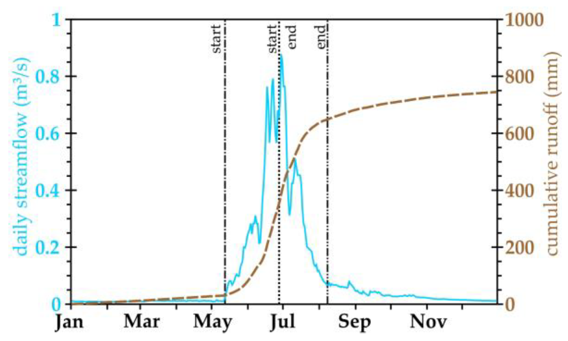
The appendix presents a sample daily hydrograph (Figure A1) to demonstrate the timing of the start, end and 50% of snowmelt contribution to flow, as per the method of Pfohl and Fassnacht [1].
Figure A1.
Sample daily (blue) and cumulative (brown) hydrograph for the Michigan River gauging stations in northern Colorado for 1993, illustrating the timing of the start (tQstart as a dashed vertical line with single dot) and end (tQend as a dashed vertical line with double dot) of the snowmelt contribution to streamflow, and the timing of 50% of flow between tQstart and tQend (tQstart-end as a dotted vertical line). The cumulative runoff is the sum of the daily streamflow divided by the area of the basin to yield a depth of water.
Appendix B. Station Summary
This appendix presents the location and areas for each study watershed (Table A1).

Table A1.
Name, USGS station number, latitude, longitude and gauge elevation, and basin area for the 39 gauges presented in Figure 1.
Table A1.
Name, USGS station number, latitude, longitude and gauge elevation, and basin area for the 39 gauges presented in Figure 1.
| name | number | latitude (o) | longitude (o) | gauge elevation (m) | basin area (km2) |
| Joe Wright Creek | 06746095 | 40.540 | -105.883 | 3045 | 8 |
| Michigan River | 06614800 | 40.496 | -105.865 | 3167 | 4 |
| Colorado River | 09010500 | 40.326 | -105.857 | 2667 | 165 |
| Cabin Creek | 09032100 | 39.986 | -105.745 | 2914 | 13 |
| Ranch Creek | 09032000 | 39.950 | -105.766 | 2640 | 52 |
| Vasquez Creek | 09025000 | 39.920 | -105.785 | 2673 | 72 |
| St. Louis Creek | 09026500 | 39.910 | -105.878 | 2737 | 85 |
| Fraser River | 09022000 | 39.846 | -105.752 | 2902 | 27 |
| S Fork of Williams | 09035900 | 39.801 | -106.026 | 2728 | 71 |
| Darling Creek | 09035800 | 39.797 | -106.026 | 2725 | 23 |
| Piney River | 09059500 | 39.796 | -106.574 | 2217 | 219 |
| Williams Fork | 09035500 | 39.779 | -105.928 | 2987 | 42 |
| Bobtail Creek | 09034900 | 39.760 | -105.906 | 3179 | 15 |
| East Meadow Creek | 09058800 | 39.732 | -106.427 | 2882 | 9 |
| Dickson Creek | 09058610 | 39.704 | -106.457 | 2818 | 9 |
| Freeman Creek | 09058700 | 39.698 | -106.446 | 2845 | 8 |
| Red Sandstone Creek | 09066400 | 39.683 | -106.401 | 2808 | 19 |
| Booth Creek | 09066200 | 39.648 | -106.323 | 2537 | 16 |
| Middle Creek | 09066300 | 39.646 | -106.382 | 2499 | 15 |
| Pitkin Creek | 09066150 | 39.644 | -106.303 | 2598 | 14 |
| Bighorn Creek | 09066100 | 39.640 | -106.293 | 2629 | 12 |
| Gore Creek | 09065500 | 39.626 | -106.278 | 2621 | 38 |
| Black Gore Creek | 09066000 | 39.596 | -106.265 | 2789 | 32 |
| Keystone Gulch | 09047700 | 39.594 | -105.973 | 2850 | 24 |
| Tenmile Creek | 09050100 | 39.575 | -106.111 | 2774 | 239 |
| Turkey Creek | 09063400 | 39.523 | -106.337 | 2718 | 61 |
| Wearyman Creek | 09063200 | 39.522 | -106.324 | 2829 | 25 |
| Eagle River | 09063000 | 39.508 | -106.367 | 2638 | 182 |
| Blue River | 09046600 | 39.456 | -106.032 | 2749 | 319 |
| Homestake Creek | 09064000 | 39.406 | -106.433 | 2804 | 92 |
| Missouri Creek | 09063900 | 39.390 | -106.470 | 3042 | 17 |
| Crystal River | 09081600 | 39.233 | -107.228 | 2105 | 433 |
| Halfmoon Creek | 07083000 | 39.172 | -106.389 | 2996 | 61 |
| Roaring Fork River | 09073300 | 39.141 | -106.774 | 2475 | 196 |
| Rock Creek | 07105945 | 38.707 | -104.847 | 2000 | 18 |
| Lake Fork | 09124500 | 38.299 | -107.230 | 2386 | 878 |
| Uncompahgre River | 09146200 | 38.184 | -107.746 | 2096 | 386 |
| Vallecito Creek | 09352900 | 37.478 | -107.544 | 2410 | 188 |
| Conejos River | 08245000 | 37.300 | -105.747 | 3007 | 104 |
Appendix C. Cross-Correlation of Trends, Parameters and Variables
This appendix presents the cross-correlation between the timing and volume trends across the 39 watersheds (Table A2) and between the variables/parameters used in the regression (Table A3). The cross-correlation is represented by the correlation coefficient (R).
Table A2.
Correlation coefficient between snowmelt timing and volume streamflow trends.
| tQend | tQstart-end | Q100 | Qstart | Qend | Qstart-end | |
| tQstart | 0.12 | -0.56 | 0.29 | 0.34 | 0.37 | 0.37 |
| tQend | 0.66 | 0.20 | 0.01 | 0.37 | 0.34 | |
| tQstart-end | -0.06 | -0.21 | -0.005 | -0.03 | ||
| Q100 | 0.12 | 0.89 | 0.82 | |||
| Qstart | 0.08 | -0.09 | ||||
| Qend | 0.94 |
Table A3.
Correlation coefficient between time trend variables (NDVI, winter precipitation, peak SWE) and parameters (basin mean solar radiation, basin mean elevation, basin mean slope, area, latitude, longitude).
Table A3.
Correlation coefficient between time trend variables (NDVI, winter precipitation, peak SWE) and parameters (basin mean solar radiation, basin mean elevation, basin mean slope, area, latitude, longitude).
| Winter P | Peak SWE | Solar Rad. | Elevation | Slope | Area | Latitude | Longitude | |
|---|---|---|---|---|---|---|---|---|
| NDVI | 0.43 | -0.13 | 0.04 | -0.06 | -0.05 | -0.06 | 0.40 | 0.13 |
| Winter P | 0.29 | 0.31 | 0.17 | -0.14 | -0.30 | 0.59 | 0.46 | |
| Peak SWE | -0.10 | 0.42 | 0.09 | -0.04 | 0.25 | 0.02 | ||
| Solar Rad. | 0.14 | -0.01 | -0.45 | 0.33 | 0.36 | |||
| Elevation | 0.44 | -0.03 | 0.19 | 0.20 | ||||
| Slope | 0.13 | -0.01 | -0.26 | |||||
| Area | -0.46 | -0.57 | ||||||
| Latitude | 0.45 |
References
- Pfohl, A.K.D.; Fassnacht, S.R. Evaluating Methods of Streamflow Timing to Approximate Snowmelt Contribution in High-Elevation Mountain Watersheds. Hydrology 2023, 10(4), 75. [CrossRef]
- Viviroli, D.; Kummu, M.; Meybeck, M.; Kallio, M.; Wada, Y. Increasing dependence of lowland populations on mountain water resources. Nature Sustainability 2020, 3(11), 917-928. [CrossRef]
- Serreze, M.C.; Clark, M.P.; Armstrong, R.L. Characteristics of the western United States snowpack from snowpack telemetry (SNOTEL) data. Water Resources Research 1999, 35(7), 2145-2160.
- Doesken, N.J.; Pielke, R.A.; Bliss, O.A.P. Climate of Colorado. Climatography of the United States No. 60; Colorado Climate Center, Atmospheric Science Department, Colorado State University, 2003. https://hdl.handle.net/10217/236290.
- Ikeda, K.; Rasmussen, R.; Liu, C.; et al. Snowfall and snowpack in the Western U.S. as captured by convection permitting climate simulations: current climate and pseudo global warming future climate. Climate Dynamics 2021, 57, 2191–2215. [CrossRef]
- Hammond, J.C.; Kampf, S.K. Subannual streamflow responses to rainfall and snowmelt inputs in snow-dominated watersheds of the western United States. Water Resources Research 2020, 56, e2019WR026132. [CrossRef]
- Cayan, D.R.; Kammerdiener, S.A.; Dettinger, M.D.; Caprio, J.M.; Peterson, D.H. Changes in the onset of spring in the western United States. Bulletin of the American Meteorological Society 2001, 82, 399-415.
- Viviroli, D., Archer, D. R., Buytaert, W., Fowler, H. J., Greenwood, G. B., Hamlet, A. F., Huang, Y., Koboltschnig, G., Litaor, M. I., López-Moreno, J. I., Lorentz, S., Schädler, B., Schreier, H., Schwaiger, K., Vuille, M., Woods, R. Climate change and mountain water resources: overview and recommendations for research, management and policy. Hydrol. Earth Syst. Sci. 2011, 15, 471-504. [CrossRef]
- Schlaepfer, D.R.; Lauenforth, W.K.; Bradford, J.B. Consequences of declining snow accumulation for water balance of mid-latitude dry regions. Global Change Biology 2012, 18, 1988-1997.
- Barnhart, T.B.; Tague, C.L.; Molotch, N.P. The counteracting effects of snowmelt rate and timing on runoff. Water Resources Research 2020, 56, e2019WR026634. [CrossRef]
- Burn, D. H.; Whitfield, P.H. Shifting cold regions streamflow regimes in North America affect flood frequency analysis. Hydrological Sciences Journal 2024. [CrossRef]
- Leung, L.R.; Qian, Y.; Bian, X.; Washington, W.M.; Han, J.; Roads J.O. Mid-century ensemble regional climate change scenarios for the western United States. Climatic Change 2004, 62, 75-113.
- Stewart, I.T.; Cayan, D.R.; Dettinger, M.D. Changes toward earlier streamflow timing across Western North America, Journal of Climate 2005, 18, 1136-1155.
- Stewart, I.T. Changes in snowpack and snowmelt runoff for key mountain regions, Hydrological Processes 2009, 23, 78-94.
- Clow, D W. Changes in timing of snowmelt and streamflow in Colorado: A response to recent warming. Journal of Climate 2010, 23, 2293-2306.
- Harpold, A.; Brooks, P.; Rajagopal, S.; Heidbuchel, I.; Jardine, A.; Stielstra, C. Changes in snowpack accumulation and ablation in the intermountain west. Water Resources Research 2012, 48, W11501. [CrossRef]
- Court, A. Measures of Streamflow Timing. Journal of Geophysical Research 1962, 67(11), 4335-4339.
- Johnson, F.A. Comments on paper by Arnold Court, ‘Measures of streamflow timing.’ Journal of Geophysical Research 1964, 69, 3525-3527.
- Satterlund, D.R.; Eschner, A.R. Land use, snow, and streamflow regimen in central New York. Water Resources Research 1965, 1(3), 397-405.
- Fassnacht, S.R. Upper versus lower Colorado River sub-basin streamflow: characteristics, runoff estimation, and model simulation. Hydrological Processes 2006, 20, 2187-2205. [CrossRef]
- Stewart, I.T.; Cayan, D.R.; Dettinger, M.D. Changes in snowmelt runoff timing in western North America under a ‘Business as Usual’ climate change scenario. Climatic Change 2024, 62, 217-232.
- Rauscher, S.A.; Pal, J.S.; Diffenbaugh, N.S.; Benedetti, M.M. Future changes in snowmelt-driven runoff timing over the western US. Geophysical Research Letters 2008, 35. [CrossRef]
- Dudley, R.W.; Hodgkins, G.A.; McHale, M.R.; Kolian, M.J.; Renard, B. Trends in snowmelt-related streamflow timing in the conterminous United States. J. Hydrol. 2017, 547, 208–221.
- Whitfield, P.H. Is ‘Centre of Volume’ a robust indicator of changes in snowmelt timing? Hydrological Processes 2013, 27, 2691-2698.
- Al Sawaf, M.B.; Kawanisi, K. Assessment of mountain river streamflow patterns and flood events using information and complexity measures. Journal of Hydrology 2020, 590, 125508. [CrossRef]
- Gordon, B.L.; Brooks, P.D.; Krogh, S.A.; Boisrame, G.F.S.; Carroll, R.W.H.; McNamara, J.P.; Harpold, A.A. Why does snowmelt-driven streamflow response to warming vary? A data-driven review and predictive framework. Environmental Research Letters 2022, 17(5), 053004. [CrossRef]
- Julander, R.P.; Curtis, J.; Beard, A. The SNOTEL temperature dataset. Mountain Views Newsletter 2007, 1(2), 4–7, available at https://www.nrcs.usda.gov/wps/PA_NRCSConsumption/download?cid=stelprdb1268403&ext=pdf.
- Oyler, J.W.; Dobrowski, S.Z.; Ballantyne, A.P.; Klene, A.E.; Running, S.W. Artificial amplification of warming trends across the mountains of the western United States Geophysical Research Letters 2015. [CrossRef]
- Ma, C.; Fassnacht, S.R.; Kampf, S.K. How temperature sensor change affects warming trends and modeling: an evaluation across the state of Colorado. Water Resources Research 2019, 55, 9748–9764. [CrossRef]
- United States Geological Survey. National Water Information System: Web Interface. United States Department of the Interior USGS Water Data for USA; http://waterdata.usgs.gov/nwis/ last accessed 12 November 2024.
- Theil, H. A rank-invariant method of linear and polynomial regression analysis. Proc. R. Neth. Acad. Sci. 1950, 53, 386–392.
- Sen, P.K. Estimates of the Regression Coefficient Based on Kendall’s Tau. Am. Stat. Assoc. J. 1968, 63, 1379–1389.
- Mann, H.B. Nonparametric Tests Against Trends. Econometrica 1945, 13, 245–259.
- Kendall, M.; Gibbons, J.D. Rank Correlation Methods, 5th ed.; Edward Arnold: London, UK, 1990.
- PRISM Climate Group. PRISM Climate Data. Northwest Alliance for Computational Science & Engineering; Oregon State University 2024. https://prism.oregonstate.edu/ (last accessed 13 November 2024).
- Meromy, L.; Molotch, N.P.; Link, T.E.; Fassnacht, S.R.; Rice, R. Subgrid variability of snow water equivalent at operational snow stations in the western USA. Hydrological Processes 2013, 27, 2382-2400. [CrossRef]
- U.S. Geological Survey. EarthExplorer. U.S. Department of Interior; <https://earthexplorer.usgs.gov/> (last accessed 13 November 2024).
- Wehner, C.E.; Stednick, J.D. Effects of mountain pine beetle-killed forests on source water contributions to streamflow in headwater streams of the Colorado Rocky Mountains. Front. Earth of Science 2017, 11, 496-504. [CrossRef]
- Kampf, S. K.; McGrath, D.; Sears, M. G.; Fassnacht, S. R.; Kiewiet, L.; Hammond, J. C. Increasing wildfire impacts on snowpack in the western US. Proceedings of the National Academy of Sciences 2022, 119(39), e2200333119.
- NRCS. Natural Resources Conservation Service. U.S. Department of Agriculture; https://www.nrcs.usda.gov/ (last accessed on 27 November 2024).
- Kilmister, I.F.; Campbell, P.; Dee, M. Till the End. Chapter 9 in Bad Magic; UDR GmbH 2015, Husum Germany.
- Winstral, A.; Elder, K.; Davis, R.E. Spatial Snow Modeling of Wind-Redistributed Snow Using Terrain-Based Parameters. J. Hydrometeorol. 2002, 3, 524–538.
- Von Thaden, B.C. Spatial Accumulation Patterns of Snow Water Equivalent in the Southern Rocky Mountains. Unpublished M.S. thesis 2016, Watershed Science, Colorado State University, Fort Collins, Colorado, USA, 52pp + 1 appendix. http://hdl.handle.net/10217/173515.
- Whitfield, P. H.; Shook, K. R. Changes to rainfall, snowfall, and runoff events during the autumn–winter transition in the Rocky Mountains of North America. Canadian Water Resources Journal/Revue canadienne des Ressources Hydriques 2020, 45(1), 28-42.
- Meiman, J.R. Snow accumulation related to elevation, aspect, and forest canopy. In Proceedings of the Snow Hydrology Workshop Seminar, Fredericton, NB, Canada, 28–29 February 1968; pp. 35–47.
- Fassnacht, S.R.; Dressler, K.A.; Bales, R.C. Snow water equivalent interpolation for the Colorado River Basin from snow telemetry (SNOTEL) data. Water Resour. Res. 2003, 39, 1208.
- Daly, S.F.; Davis, R.; Ochs, E.; Pangburn, T. An approach to spatially distributed snow modelling of the Sacramento and San Joaquin basins, California. Hydrological Processes 2000, 14, 3257–3271.
- Dawson, N.; Broxton, P.; Zeng, X. Evaluation of Remotely Sensed Snow Water Equivalent and Snow Cover Extent over the Contiguous United States. J. Hydrometeor. 2018, 19, 1777–1791. [CrossRef]
- Hammond, J.C.; Sexstone, G.A.; Putman, A.L.; Barnhart, T.B.; Rey, D.M.; et al. High Resolution SnowModel Simulations Reveal Future Elevation-Dependent Snow Loss and Earlier, Flashier Surface Water Input for the Upper Colorado River Basin. Earth’s Future 2023, 11, e2022EF003092. [CrossRef]
- Helsel, D.R.; Frans, L.M. Regional Kendall test for trend. Environ. Sci. Technol 2006., 40, 4066–4070.
- Fassnacht, S. R.; Cherry, M. L.; Venable, N. B. H.; Saavedra, F. Snow and albedo climate change impacts across the United States Northern Great Plains. The Cryosphere 2016, 10, 329–339. [CrossRef]
- Gómez-Landesa, E.; Rango, A. Operational snowmelt runoff forecasting in the Spanish Pyrenees using the snowmelt runoff model. Hydrol. Process. 2002, 16, 1583-1591. [CrossRef]
- Painter, T.H.; Skiles, S.M.; Deems, J.S.; Brandt, W.T.; Dozier, J. Variation in Rising Limb of Colorado River Snowmelt Runoff Hydrograph Controlled by Dust Radiative Forcing in Snow. Geophys. Res. Lett. 2018, 45, 797–808.
- Doskocil, L.G.; Fassnacht, S.R.; Barnard, D.M.; Pfohl, A.K.D.; Derry, J.E.; Sanford, W.E. Twin-Peaks Streamflow Timing: Can We Use Forest and Alpine Snow Melt-Out Response to Estimate? Water 2025, 17, 2017. [CrossRef]
- Flynn, H.; Fassnacht, S.R.; MacDonald, M.S.; Pfohl, A.K.D. Baseflow from Snow and Rain in Mountain Watersheds. Water 2024, 16, 1665. [CrossRef]
- Eckhardt, K. How to construct recursive digital filters for baseflow separation. Hydrol. Process. 2005, 19, 507-515. [CrossRef]
- Taylor, S.; Feng, X.; Williams, M.; McNamara, J. How isotopic fractionation of snowmelt affects hydrograph separation. Hydrol. Process. 2002, 16, 3683-3690. [CrossRef]
- Miller, M.P.; Susong, D.D.; Shope, C.L.; Heilweil, V.M.; Stolp, B.J. Continuous estimation of baseflow in snowmelt-dominated streams and rivers in the Upper Colorado River Basin: A chemical hydrograph separation approach. Water Resources Research 2014, 50, 6986–6999. [CrossRef]
- Bates, C.G.; Henry, A. J. Second Phase of Streamflow Experiment at Wagon Wheel Gap, Colo. Monthly Weather Review 128, 56, 79–80. [CrossRef]
- Wilm, H.G.; Dunford, E.G. Effect of timber cutting on water available for stream flow from a lodgepole pine forest. Department of Agriculture 1948, Report No. 968.
- OpenET. OPEN ET – Filling the Biggest Data Gap in Water Management 2025; https://etdata.org/ (last accessed on 27 June 2025).
Figure 1.
Distribution of gauging stations across Colorado in the Southern Rocky Mountains.
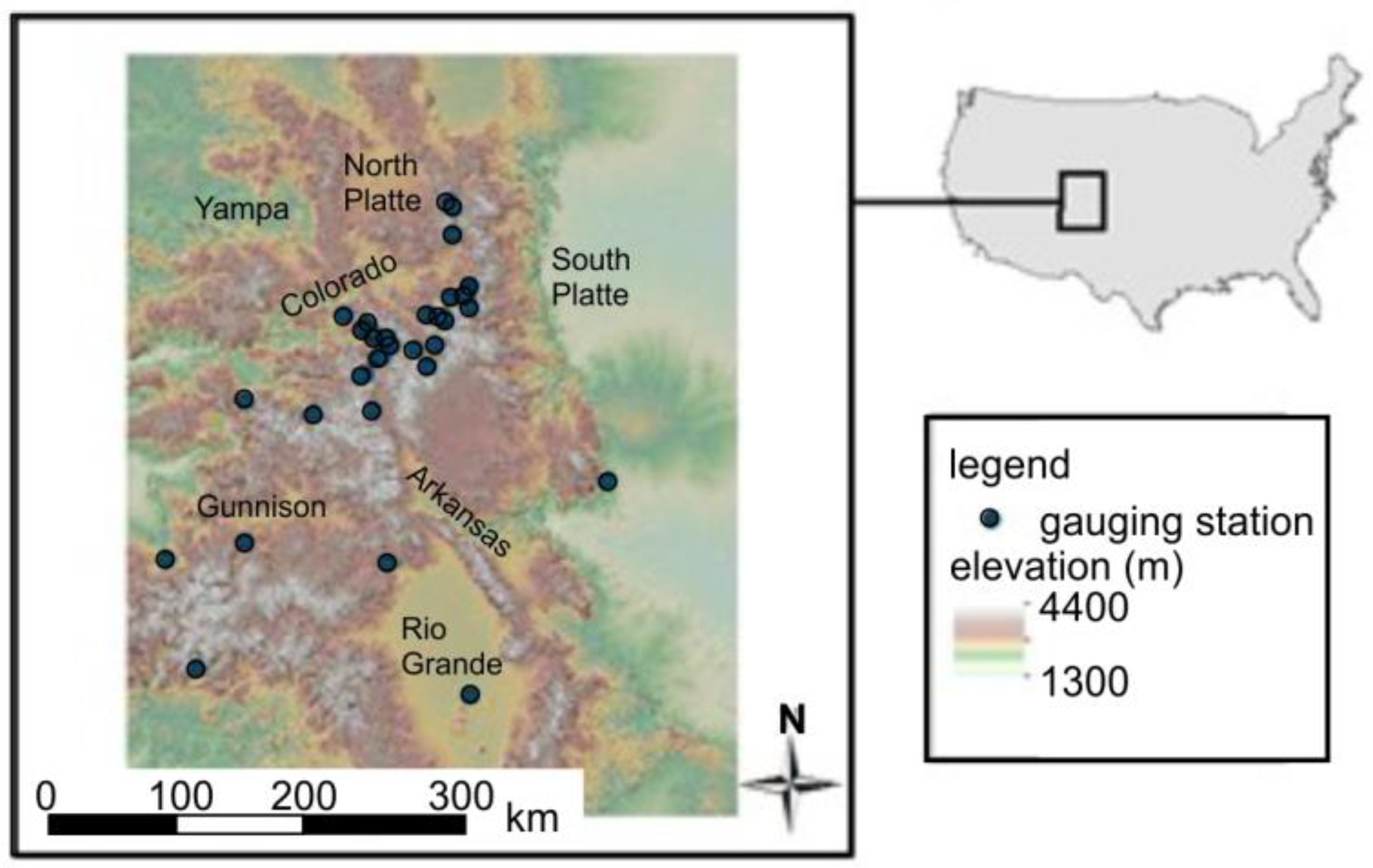
Figure 2.
Study watershed parameters of (a) mean basin elevation, (b) mid-April clear sky solar radiation input, (c) slope, and (d) basin area (logarithmic scale). The time trend in the (e) NDVI, (f) winter precipitation, and (g) peak SWE from the near SNOTEL station. The watersheds are ordered from top to bottom by latitude with horizontal dashed lines separating the basins by proximity, as per Figure 1. Bars with solid outlines are statistically significant trends at p < 0.05 and dashed bars are moderately significant at p <0.1 (in e, f, g).
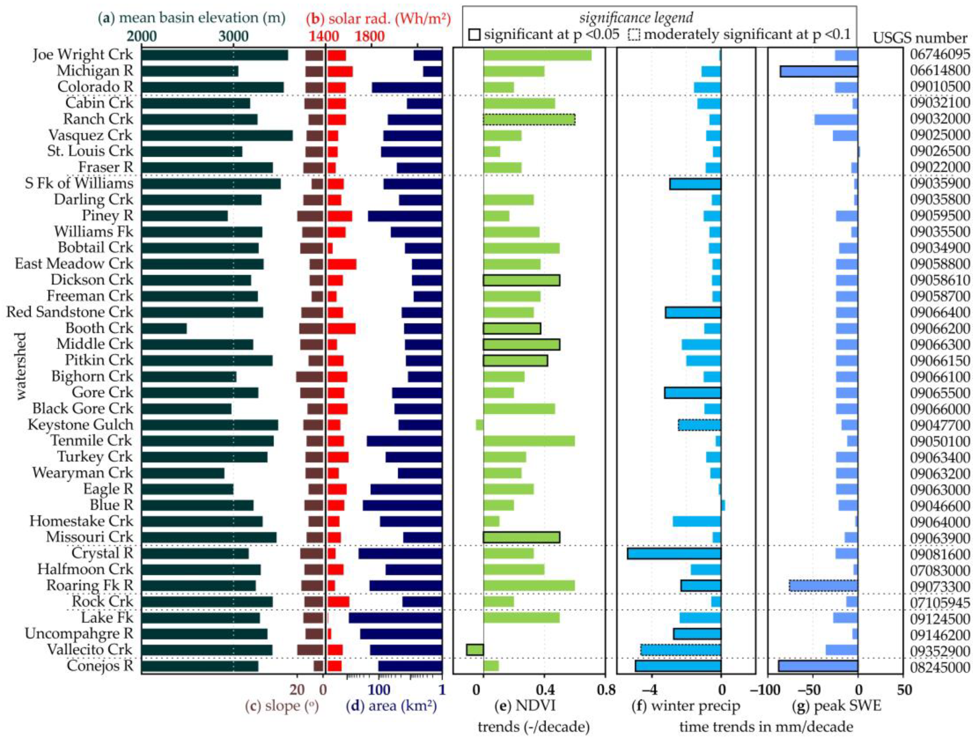
Figure 3.
Trends in the streamflow timing (a) tQstart, (b) tQend, (c) tQstart-end), and volume (d) Q100, (e) Qstart, (f) Qend, and (g) Qstart-end) across the 39 study basins. Bars with solid outlines are statistically significant trends at p < 0.05 and dashed bars are moderately significant at p <0.1.
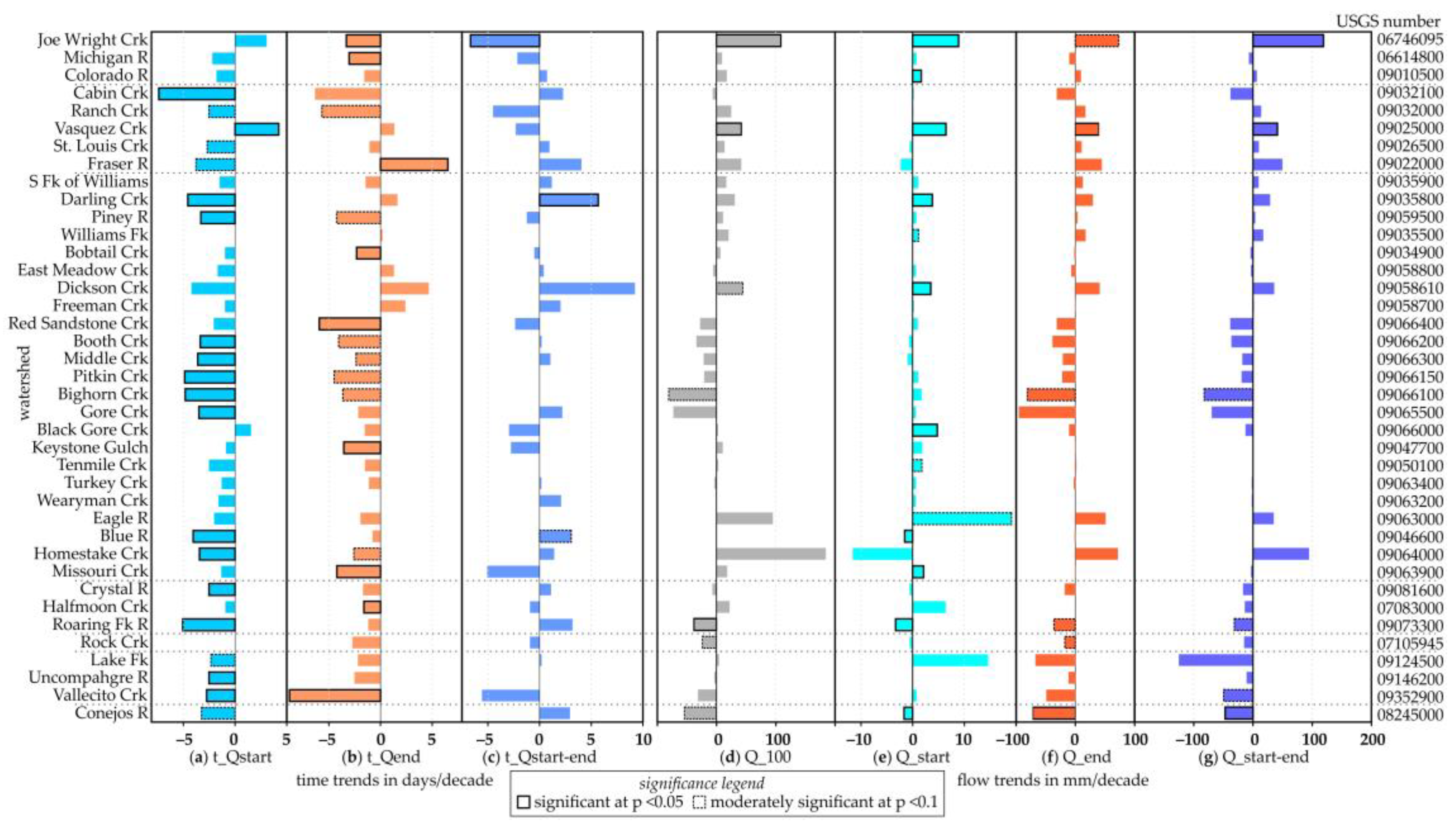
Figure 4.
Correlation between streamflow timing (t_Qstart, t_Qend, t_Qstart-end) or volume (Q_100, Q_start, Q_end, Q_start-end) trends and changes in time trends in NDVI, winter precipitation, peak SWE, or watershed terrain parameters (mean radiation, mean elevation, mean slope, basin area, latitude, longitude) across the 39 study basins.
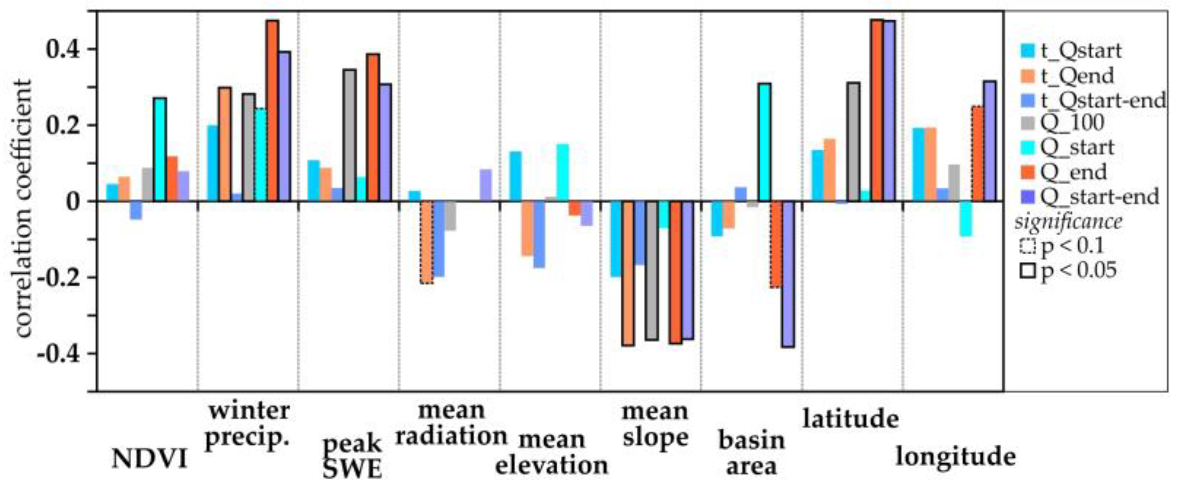
Table 1.
Linear multi-variate regression results for (a) regression with all variables (NDVI, winter precipitation, peak SWE) and parameters (basin mean solar radiation, basin mean elevation, basin mean slope, area, latitude, longitude), (b) regression with winter precipitation, slope and latitude, and (c) regression with winter precipitation, slope and latitude as the independent variables to estimate timing (tQstart, tQend, tQstart-end) and flow volumes (Q100, Qstart, Qend, Qstart-end). The coefficient of determination (R2) and the statistical significance are presented, with the regression coefficients. The independent variables were standardized to a value between 0 and 1. The moderately significant correlations (p<0.1) are italicized and denoted with a +; the significant correlations (p<0.05) are in bold and denoted with a *.
| Variable | R2 | Sign. F | Intercept | NDVI | Winter P | Peak SWE | Solar Rad. | Elev. | Slope | Area | Lat. | Long. |
|---|---|---|---|---|---|---|---|---|---|---|---|---|
| (a) regression with all variables/parameters | ||||||||||||
| tQstart | 0.12 | 0.91 | -1.96 | -0.306 | 0.20 | -0.003 | -0.002 | 0.002 | -0.15 | -0.0002 | 0.12 | 0.06 |
| tQend | 0.33 | 0.16 | 27.8 | -2.48 | 0.78 | -0.01 | -0.014* | -0.0004 | -0.22 | -0.0006 | 0.55 | 0.20 |
| tQstart-end | 0.10 | 0.94 | 81.7 | -1.86 | 0.17 | 0.006 | -0.009 | -0.003 | -0.05 | 0.0008 | 0.28 | 0.65 |
| Q100 | 0.37 | 0.09+ | -1990 | -12.5 | 2.57 | 0.54 | -0.062 | 0.016 | -5.41* | 0.034 | 24.8 | -11.1 |
| Qstart | 0.31 | 0.22 | -167 | 5.36 | 0.95 | -0.01 | 0.007 | 0.006 | -0.28 | 0.011+ | -0.38 | -1.47 |
| Qend | 0.52 | 0.006* | -1200 | 26.9 | 7.44 | 0.45 | -0.076 | -0.014 | -3.28* | -0.008 | 22.1* | -5.44 |
| Qstart-end | 0.56 | 0.02* | -977 | -28 | 4.10 | 0.45 | -0.066 | -0.020 | -3.27+ | -0.054 | 23.5+ | -2.86 |
| (b) regression with winter precipitation, slope and latitude | ||||||||||||
| tQstart | 0.071 | 0.45 | -5.9 | 0.23 | -0.096 | 0.15 | ||||||
| tQend | 0.21 | 0.043* | -0.03 | 0.49 | -0.25* | 0.086 | ||||||
| tQstart-end | 0.21 | 0.80 | 4.23 | 0.006 | -0.13 | -0.046 | ||||||
| Q100 | 0.23 | 0.024* | -632 | 2.64 | -4.17* | 18.2 | ||||||
| Qstart | 0.08 | 0.39 | 53.2 | 1.12 | -0.03 | -1.25 | ||||||
| Qend | 0.40 | 0.0004* | -686+ | 6.24 | -3.25* | 19.0* | ||||||
| Qstart-end | 0.36 | 0.001* | -962* | 3.16 | -3.74* | 26.1* | ||||||
| (c) regression with solar radiation, slope and latitude | ||||||||||||
| tQstart | 0.06 | 0.55 | -0.001 | -0.11 | 0.44 | |||||||
| tQend | 0.25 | 0.02* | -0.011+ | -0.27* | 1.1 | |||||||
| tQstart-end | 0.07 | 0.45 | -0.008 | -0.13 | 0.28 | |||||||
| Q100 | 0.27 | 0.01* | -0.12 | -4.3* | 25.9* | |||||||
| Qstart | 0.006 | 0.97 | -0.001 | -0.09 | 0.22 | |||||||
| Qend | 0.39 | 0.001* | -0.083 | -3.5* | 29.6 | |||||||
| Qstart-end | 0.36 | 0.001* | -0.044 | -3.9* | 31.5* | |||||||
| (d) regression with slope and latitude | ||||||||||||
| tQstart | 0.057 | 0.35 | -16.9 | -0.107 | 0.42 | |||||||
| tQend | 0.17 | 0.035* | -23.7 | -0.271* | 0.68 | |||||||
| tQstart-end | 0.028 | 0.60 | 3.94 | -0.13 | -0.039 | |||||||
| Q100 | 0.23 | 0.009* | -758+ | -4.29* | 21.3* | |||||||
| Qstart | 0.006 | 0.90 | -4.69 | -0.86 | 0.20 | |||||||
| Qend | 0.37 | 0.0003* | -984* | -3.54* | 26.4* | |||||||
| Qstart-end | 0.35 | 0.0004* | -1113* | -3.89* | 29.8* | |||||||
Disclaimer/Publisher’s Note: The statements, opinions and data contained in all publications are solely those of the individual author(s) and contributor(s) and not of MDPI and/or the editor(s). MDPI and/or the editor(s) disclaim responsibility for any injury to people or property resulting from any ideas, methods, instructions or products referred to in the content. |
© 2025 by the authors. Licensee MDPI, Basel, Switzerland. This article is an open access article distributed under the terms and conditions of the Creative Commons Attribution (CC BY) license (http://creativecommons.org/licenses/by/4.0/).
Copyright: This open access article is published under a Creative Commons CC BY 4.0 license, which permit the free download, distribution, and reuse, provided that the author and preprint are cited in any reuse.


