Submitted:
16 July 2025
Posted:
16 July 2025
You are already at the latest version
Abstract
In this paper, we introduce and investigate the BT inverse for a ring element. The binary relation BT order has also been studied. Furthermore, we introduce the generalized BT inverse and present some presentations of this new generalized inverse. It also be characterized by using system of equations and Pierce decompositions of ring elements. Many properties of BT inverse for complex matrices are generalized to a broader context within a ring.
Keywords:
core inverse
; Moore-Penrose inverse
; BT inverse
; generalized BT inverse
; BT order
; ring
1. Introduction
An associative ring with an identity 1 is called a *-ring if there exists an involution satisfying for all . An element has group inverse provided that there exists such that
Such x is unique if exists, denoted by , and called the group inverse of a. As is well known, a square complex matrix A has group inverse if and only if (see [13]). An element has core inverse if there exists some such that
If such x exists, it is unique, and denote it by  . Let represent the range space of a complex matrix X. A square complex matrix A has core inverse
  if and only if
  is a projection and
 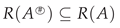 (see [3,16]). Group and core inverses are extensively studied by many authors from very different points of view, e.g., [1,3,7,10,13,16].
. Let represent the range space of a complex matrix X. A square complex matrix A has core inverse if and only if is a projection and (see [3,16]). Group and core inverses are extensively studied by many authors from very different points of view, e.g., [1,3,7,10,13,16].An element has Moore-Penrose inverse if there exists such that
The preceding x is unique if it exists, and we denote it by . The set of all Moore-Penrose invertible elements in R is denoted by . Evidently, every square complex matrix has the Moore-Penrose inverse. In [2], Baksalary and Trenkler extended core inverse and introduced a generalized core inverse. Recently, Ferreyra and Malik studied such generalized core inverse and call it the introduced BT inverse for a complex matrix. The matrix is called the BT inverse of A. Many elementary properties of this new generalized inverse are established in [5]. For additional references on the BT inverse, we refer the reader to [6,8,9,17].
The motivation of this paper is to extend the proposed generalized inverse for complex matrices to a more general setting within a ring. We introduce the BT inverse for an element in a ring R. Furthermore, we establish and prove several fundamental properties of the BT inverse within this ring.
In Section 2, we introduce a new generalized inverse as the generalization of BT inverse of a complex matrix.
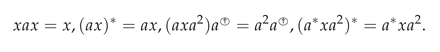
Definition 1.
An element has BT inverse if there exists such that
If such x exists, it is unique, and denote it by . The set of all BT invertible elements in R is denoted by .
In [15], based on the Hartwig-Spindelbock decomposition of a complex matrix, Wang characterize the BT inverse of a complex matrix by using the system by equations. Replacing the Hartwig-Spindelbock decomposition, we employ the Pierce representation of a ring element as a tool to extend the characterization of BT inverse of a complex matrix to a broader context within a ring. We prove that has BT inverse if and only if . In this case, . In Section 3, we investigate the order relation induced by BT inverse. Many characterizations of the BT order are obtained by using Pierce decomposition for a ring element.
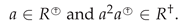
Let
Let be a Banach algebra. Evidently,
Definition 2.
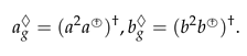
An element has generalized BT inverse if there exist such that
We denote by and call it the generalized BT inverse of a. The set of all generalized BT invertible elements in is denoted by .
Recall that an element has generalized Moore-Penrose inverse if there exists such that
The preceding x is denoted by  . The set of all generalized Moore-Penrose invertible elements in R is denoted by
  .
.
. The set of all generalized Moore-Penrose invertible elements in R is denoted by .In Section 4, we prove that if and only if 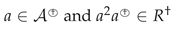 . We further characterize the generalized BT inverse by using the system of equations.
. We further characterize the generalized BT inverse by using the system of equations.Finally, in Section 5, we present certain characterizations of the generalized BT inverse for a geometrical point of view.
Throughout the paper, all rings are associative *-rings with an identity. and denote the sets of all group invertible, More-Penrose invertible and generalized Moore-Penrose invertible elements in R, respectively. Let . Set and . Let . Then . We use to denote the projection p such that and .
denote the sets of all group invertible, More-Penrose invertible and generalized Moore-Penrose invertible elements in R, respectively. Let . Set and . Let . Then . We use to denote the projection p such that and .2. BT Inverse
The purpose of this section is to investigate the elementary properties of the BT inverse, which will be frequently utilized in subsequent sections. Our starting point is as follows.
Theorem 1.
Let . Then the following are equivalent:
- (1)
- .
- (2)
- .
In this case, .
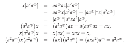
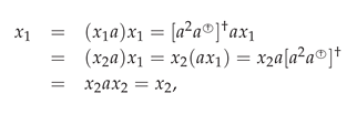
Proof. By hypothesis, there exists such that Write for a . We directly verify that
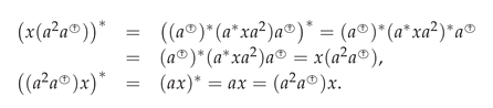
Moreover, we see that
Therefore and . This implies that x is unique, as required.
Let Then
We further check that
Therefore is the solution of the system of equations:
as required. □
Corollary 1.
Let  . Then and
  .
.
. Then and .
Proof.
In view of [16, Theorem 2.6],  .
.
.Then we have  . It is easy to verify that
 Then
Then 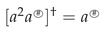 This implies that . In this case, . □
. It is easy to verify that
This implies that . In this case, . □Let and . Then we have
Lemma 1.
Let . Then and
Proof.
It is easy to verify that
Moreover, we have
Thus, .
In light of Theorem 2.1, we derive that
as asserted. □
We come now to establish the representation of the BT inverse by using certain projections.
Theorem 2.
Let . Then
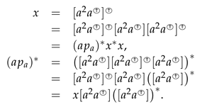
Proof.
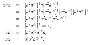
By virtue of Lemma 2.3, . Further, we verify that
Furthermore, we check that
Therefore □
Corollary 2.
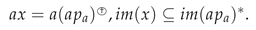
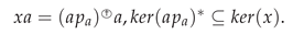
Let . The system given by
is consistent and its unique solution is
Proof.
Clearly, we have In view of Theorem 2.4, Hence, . We infer that
Suppose that
for some . As , we write for some . Then
as required. □
Theorem 3.
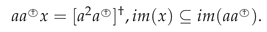
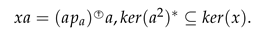
Let . The system given by
is consistent and its unique solution is
Proof.
One easily checks that
Suppose that for . Then ; hence, . Therefore , as asserted. □
Let . An element a has -inverse provide that there exists such that
If such x exists, it is unique and denote it by (see [4]).
Theorem 4.
Let . Then
Proof.
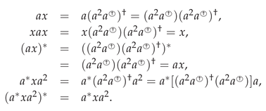
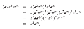
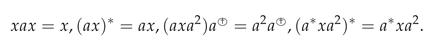
Obviously, . Let . We verify that
Therefore as asserted. □
Let and . We say that a has -inverse x provided that . We denote x by . We next consider the relation between the BT inverse and -inverse in a ring. .
Theorem 5.
Let . Then
Proof.
Let . Clearly, we have .
Step 1. . In view of Theorem 2.1, we have
Hence, . Therefore .
Step 2. . If for some , then
Hence, .
If , then
Thus, , as required.
Therefore we complete the proof. □
3. BT Order
This section is devoted to the BT order for two elements is a ring. Let and .
Definition 3.
We say that if and only if
Let . Then we have
Moreover, we compute that
Theorem 6.
Let . Then the following are equivalent:
- (1)
- .
- (2)
- There exist such that a and b are represented bywhere .
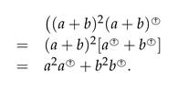
Proof. Since , we see that
Write . Then
By hypothesis, we have
Hence, .
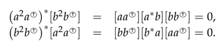
Since , we directly verify that
Therefore , as desired. □
Corollary 3.
Let and . Then the following are equivalent:
- (1)
- .
- (2)
- There exists such that a and b are represented bywhere .
- (3)
Proof. This is obvious by Theorem 3.2.
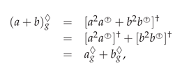
By hypothesis, we have ; hence, . This implies that . Since we verify that
as desired.
Write . By hypothesis, we have
Hence,
This implies that and then
Since , we deduce that . This implies that , and so .
Moreover, we have
Hence and so
Therefore , as required. □
Corollary 4.
Let and . Then the following are equivalent:
- (1)
- .
- (2)
- .
- (3)
- .
Proof. In view of Corollary 3.3,
where . Thus, , as required.
In view of Theorem 3.2, . Set . Then , and so
By using Corollary 3.3, .
By hypothesis, we have
Hence, Thus , as required.
Since and , we derive that as desired. □
We are ready to prove:
Theorem 7.
Let and . If then .
Proof.
In view of Theorem 3.2, we have
where . Since , we see that
This implies that .
In view of Lemma 2.3, Therefore
By hypothesis, we compute that
Therefore
Accordingly, . □
Corollary 5.
Let and . If if and only if .
Proof.
⟸ Since , as in the proof in Theorem 3.5, we deduce that
hence, . This implies that
It follows that . Thus . Since , we have ; whence, . Thus . Accordingly, , as required.
⟸ This is proved in Theorem 3.5. □
4. Generalized BT Inverse
The aim of this section is to introduce the notion of the generalized BT inverse in a ring. For further use, we formally establish the following lemma:
Lemma 2.
Let . Then the following are equivalent:
- (1)
- .
- (2)
- There exist such that
Proof. By hypotheses, there exists such that
Set and Then . We claim that x has Moore-Penrose inverse. Evidently, we verify that
Therefore and .
Moreover, we see that
Since , we have
By hypothesis, we get . Therefore there exists the Moore-Penrose decomposition , as required.
By hypothesis, there exist such that
Set . One easily checks that
Moreover, we check that
and then Then
Since , we see that
Therefore , as asserted. □
, as asserted. □
Theorem 8.
Let . Then the following are equivalent:
- (1)
- .
- (2)
In this case,
Proof. Since , there exist such that
Clearly, . In light of Lemma 4.1, and . It is easy to verify that
and . It is easy to verify that
Moreover, we check that 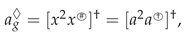 as required.
as required.
Since , by virtue of Lemma 4.1, there exist such that
, by virtue of Lemma 4.1, there exist such thatIn this case, . Moreover, we have 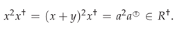 Therefore . Accordingly, . □
. Moreover, we have Therefore . Accordingly, . □As an immediate consequence, we derive
Corollary 6.
Let . Then the following are equivalent:
- (1)
- .
- (2)
- The system of conditionsis consistent and it has the unique solution.
In this case,
Corollary 7.
Let . If , then . In this case,
Proof.
Since , it follows by Theorem 4.2 that 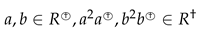 and
and
and
Since , we verify that 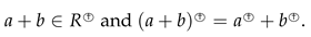 It is easy to verify that
It is easy to verify that
By hypothesis, we verify that
In light of Theorem 4.2,
 as asserted. □
We are ready to prove:
Theorem 9.
Let . Then if and only if
- (1)
- ;.
- (2)
- there exists
 such that
In this case,
Proof.
⟹ Let  We verify that
We verify that
Furthermore, we have
 as required.
⟸ By hypothesis, there exists  such that
such that
Write 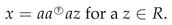 Then we check that
Then we check that
Moreover, we see that
Therefore 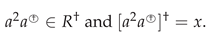 This completes the proof. □
This completes the proof. □
Corollary 8.
Let . Then if and only if . In this case,
Proof.
⟹ This is obvious.
⟸ Since , we have . In view of Theorem 4.5, there exists such that
. In view of Theorem 4.5, there exists such that
Hence,
Therefore . In this case, , as asserted. □
5. Characterizations of the Generalized BT-Inverse
The main purpose of this section is to provide new properties of the generalized BT-inverse in a ring. Consider the system given by
Lemma 3.
If the system of equations has a solution, then it is unique.
Proof.
Assume that satisfy . Then
 for . Therefore
 as desired. □
Theorem 10.
Let . Then the following are equivalent:
- (1)
- .
- (2)
- The system of equations is consistent and it has the unique solution x.
Proof. Taking In view of Theorem 4.2,  Then
Then
Then
By virtue of Lemma 5.1, x is the unique solution of the preceding equations, as required.
By the argument above, we have  Therefore by Theorem 4.2. □
Therefore by Theorem 4.2. □We are ready to prove:
Theorem 11.
Let . Then the following are equivalent:
- (1)
- .
- (2)
- (3)
- (4)
- (5)
Proof. In view of Theorem 5.2, 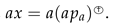 We verify that
 as required.
We verify that
Write for a . Then
 as required.
In view of Theorem 4.2,  Then we easily check that
Then we easily check that
Write  for a . Then
for a . Then
By virtue of Theorem Theorem 4.2, , as desired.
Obviously, 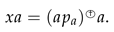 If , then . Hence,
 Thus . That is, , as desired.
If , then . Hence, Thus . That is, , as desired.
We directly verify that , as required.
As  we get . Hence, . Since , we have . Therefore
we get . Hence, . Since , we have . Therefore
Therefore we complete the proof by Theorem 4.2. □
Corollary 9.
Let . Then the following are equivalent:
- (1)
- .
- (2)

Proof. In view of Theorem 5.1, . Moreover, we have
It is easy to verify that
Hence, . Obviously, 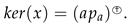 . Thus, we have
 as required.
. Thus, we have
By hypothesis,  Then
Then  Moreover, we have
  According to Theorem 5.3, we complete the proof. □
Then Moreover, we have According to Theorem 5.3, we complete the proof. □
Theorem 12.
Let . Then
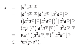
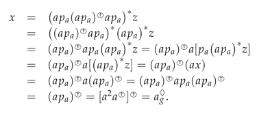
Proof.
Set . In view of Theorem 5.2, we have .
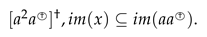
Step 1. . In view of Theorem 4.2, we have
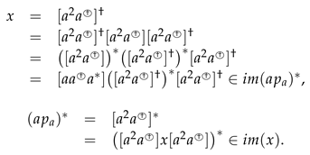
Accordingly, we have .
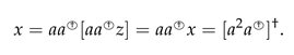
Step 2. . If for some , then
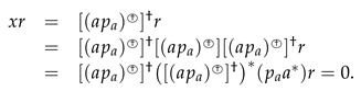
Thus .
If , then
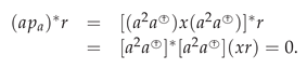
Thus, . As a result, we have .
Therefore By the similar way, we check that This completes the proof. □
References
- O.M. Baksalary and G. Trenkler, Core inverse of matrices, Linear Multilinear Algebra, 58(2010), 681–697. [CrossRef]
- O.M. Baksalary and G. Trenkler, On a generalized core inverse, Applied Math. Comput., 236(2014), 450–457. [CrossRef]
- J. Chen; H. Zhu; P. Patricio and Y. Zhang, Characterizations and representations of core and dual core inverses, Canad. Math. Bull., 2016. [CrossRef]
- M.P. Drazin, A class of outer generalized inverses, Linear Multilinear Algebra, 436 (2012), 1909–1923. [CrossRef]
- D.E. Ferreyra and S.B. Malik, The BT inverse, In book: Generalized Inverses: Algoritms and Applications, Publisher: Nova Science Publishers, 2021.
- D.E. Ferreyra; N. Thome and C. Torigino, The W-weighted BT inverse, Quest. Math., 46(2023), 359–374. [CrossRef]
- T. Li and J. Chen, Characterizations of core and dual core inverses in rings with involution, Linear Multilinear Algebra, 66(2018), 717–730. [CrossRef]
- W, Jiang and K. Zuo, Revisiting of the BT-inverse of matrices, AIMS Math., 6(2021), 2607–2622. [CrossRef]
- A. Kara; N. Thome and D.S. Djordjević, Simultaneous extension of generalized BT-inverses and core-EP inverses, Filomat, 38(2024), 10605–10614.
- N. Mihajlovic, Group inverse and core inverse in Banach and C*-algebras, Comm. Algebra, 48(2020), 1803–1818. [CrossRef]
- D. Mosić, Weighted generalized Moore-Penrose inverse, Georgian Math. J., 30(2023), 919–932.
- K.S. Stojanović and D. Mosić, Generalization of the Moore-Penrose inverse, Rev. R. Acad. Cienc. Exactas Fis. Nat., Ser. A Mat., 114(2020), No. 4, Paper No. 196, 16 p.
- D.S Rakic; N.C. Dincic and D.S. Djordjevic, Group, Moore-Penrose, core and dual core inverse in rings with involution, Linear Algebra Appl., 463(2014), 115–133. [CrossRef]
- H. Wang, Core-EP Decomposition and its applications, Linear Algebra Appl., 508(2016), 289–300. [CrossRef]
- H. Wang, Some new characterizations of generalized inverses, Front. Math., 18(2023), 1397–1402. [CrossRef]
- S. Xu; J. Chen and X. Zhang, New characterizations for core inverses in rings with involution, Front. Math., 2017. [CrossRef]
- S. Xu and D. Wang, New characterizations of the generalized B-T inverse, Filomat, 36(2022), 945–950.
Disclaimer/Publisher’s Note: The statements, opinions and data contained in all publications are solely those of the individual author(s) and contributor(s) and not of MDPI and/or the editor(s). MDPI and/or the editor(s) disclaim responsibility for any injury to people or property resulting from any ideas, methods, instructions or products referred to in the content. |
© 2025 by the authors. Licensee MDPI, Basel, Switzerland. This article is an open access article distributed under the terms and conditions of the Creative Commons Attribution (CC BY) license (http://creativecommons.org/licenses/by/4.0/).
Copyright: This open access article is published under a Creative Commons CC BY 4.0 license, which permit the free download, distribution, and reuse, provided that the author and preprint are cited in any reuse.


