

Submitted:
15 July 2025
Posted:
16 July 2025
You are already at the latest version
Abstract
First, using the principal component analysis (PCA) approach, we construct an investor attention index from seven variables: abnormal trading volume, extreme returns, past returns, nearness to the 52-week high, nearness to the historical high, Google search volume, and mutual fund inflows. Second, this study examines the impact of the investor attention index on the KSE-100 index excess returns. For this purpose, we collect monthly data from January 2004 to December 2024. The PCA identified four components and constructed attention indices: has highest weights of nearness to the 52-week high, abnormal trading volume, past returns, and mutual funds inflows; has major weights of abnormal trading volume, extreme returns, past returns, and Google search volume; has nearness to the 52-week high, nearness to the historical high, extreme returns, and mutual funds inflows and has nearness to the historical high, extreme returns, Google search volume, and mutual funds inflows. The , and have a positive and significant impact on the excess returns of the KSE-100 index. This suggests that when investors are more motivated to invest, herding behavior increases, leading to improved index performance and higher returns. Subsequently, has a negative but significant impact on index returns, indicating that a lack of investor interest leads to reduced trading activity and weaker index performance. The findings of this study have important implications for policymakers, investors, and mutual fund managers to understand the patterns of investor attention, creating policies and procedures to make the financial markets more transparent and protect the investor’s rights.
Keywords:
investor attention
; stock market returns
; KSE-100 index
; principal component analysis
has highest weights of nearness to the 52-week high, abnormal trading volume, past returns, and mutual funds inflows; has major weights of abnormal trading volume, extreme returns, past returns, and Google search volume; has nearness to the 52-week high, nearness to the historical high, extreme returns, and mutual funds inflows and has nearness to the historical high, extreme returns, Google search volume, and mutual funds inflows. The , and have a positive and significant impact on the excess returns of the KSE-100 index. This suggests that when investors are more motivated to invest, herding behavior increases, leading to improved index performance and higher returns. Subsequently, has a negative but significant impact on index returns, indicating that a lack of investor interest leads to reduced trading activity and weaker index performance. The findings of this study have important implications for policymakers, investors, and mutual fund managers to understand the patterns of investor attention, creating policies and procedures to make the financial markets more transparent and protect the investor’s rights.
1. Introduction
Investor attention has long been a subject of interest in financial research, particularly as markets increasingly exhibit patterns that deviate from traditional rational models. One such deviation arises from the concept of investor attention, defined as a limited cognitive resource that influences how individuals process information and make investment decisions. Contrary to the Efficient Market Hypothesis (Fama, 1970), which assumes that all available information is fully and instantly reflected in asset prices, behavioral finance suggests that investors often rely on selective attention, shaped by information overload, media signals, and cognitive limitations (Kahneman, 1973; Barber & Odean, 2008; Peng & Xiong, 2006). This limited attention can cause disproportionate focus on certain stocks ormarket-wide events, leading to price fluctuations that are not entirely justified by fundamentals. While a growing body of literature supports the link between investor attention and predictability of stock return in developed markets (Da, Engelberg, & Gao, 2011; Li & Yu, 2012), evidence from emerging economies remains fragmented. This study contributes to the discourse by examining the impact of investor attention on Pakistan’s KSE-100 Index performance, where structural reforms, evolving investor attention, and heightened volatility create a compelling environment for such analysis.
In Pakistan, initially, there were three stock exchanges: the Karachi Stock Exchange (KSE), the Lahore Stock Exchange (LSE), and the Islamabad Stock Exchange (ISE). The existence of each stock exchange raised a conflict of interest and frustration for the investors, as all three exchanges had no mutual coordination and were functioning separately in terms of trading interfaces, indexes, and listing criteria. Hence, the government of Pakistan introduced the Stock Exchanges Act in 2012, integrated all three stock exchanges into one operation, and formed the “Pakistan Stock Exchange” (PSX) on January 11, 2016. It became functional with the beginning of 559 listed companies from 35 sectors, including domestic and foreign companies. The history of PSX has witnessed a significant improvement over the time. It started with just five listed companies with a total paid-up capital of Rs 37 million. Then, in the 1960s, 81 companies were added with a free-float capitalization of Rs 1.8 billion. The PSX witnessed an aggregate market capitalization of Rs 10.37 trillion as of June 30, 2024.
Among the indices operating under the PSX, the performance of the KSE-100 index is reflected as a barometer to evaluate the country’s economic progress. The KSE-100 index was brought into effect in November 1991. The base value was set at 1000 points. As the number in the index suggests, it comprises 100 blue-chip companies. The criteria for selecting companies for the KSE 100 index are based on two main components: Sectorial Representation and companies with the highest free float market capitalization. Initially, 35 companies are selected from 36 available sectors (one from each sector) based on the highest free float capitalization (the Open-End Mutual Fund Sector is excluded). The remaining 65 companies are chosen based on the highest free-float capitalization, irrespective of their sector. Hence, the KSE-100 Index comprises about 80% of the total free float market capitalization of all listed companies on the Exchange. The rationale for selecting the KSE 100 Index includes: the broad market coverage, sectoral diversity, and economic importance. Other than reflecting the collective movements of major publicly traded firms in Pakistan, it is a barometer of national economic performance and is a critical tool for investors, analysts, and policymakers. With its comprehensive composition, researchers can draw insightful and meaningful inferences about the macroeconomic trends, the behavior of the investors, and the movement of the financial market in the Pakistani context.
Figure 1 shows the KSE-100 price index data from January 2004 through December 2024. The data was extracted from LSEG (Formerly Refinitiv and Thomson Reuters) DataStream. The figure shows that the Index witnessed a huge financial crash in 2008, wherein the market stopped working for four months after a minor crash in 2005. The military ruling ended in 2008, and the power was transferred to a civil democratic government. After the financial crisis of 2008, many discussions were made to make changes in the stock market. Finally, a new Act was enacted in 2012, named the Corporatization, Demutualization, and Integration Stock Exchanges Act. Resultantly, on the 27th of August 2012, the process of corporatization and demutualization began. The PSX was reflected as the best performer among the world’s equity markets between 2009 and 2016 (Shafique et al., 2019). Reflecting this milestone, Bloomberg ranked the Pakistani index among the five best stock performers in 2016 (Mangi, 2016). It is also considered an emerging secondary market by the FTSE. In 2017, it was again classified by MSCL (Morgan Stanley Capital International) and NBSP as an emerging market. The economy witnessed a boom, and PSX performed best due to high Chinese Investment in CPEC projects from 2013 to 2018. However, in May 2017, the market showed a bearish trend, and the Index dropped by 28% as an association of China purchased 40% of the shares for $ 85 million. The year 2018 showed mixed trends, while PSX’s performance fell in August 2019 due to the US-China war and the Kashmir dispute between Pakistan and India (Shafique et al., 2019).
Interestingly, in 2020, out of 61 stock exchanges in the world, the PSX secured its position as the fourth best-performing stock exchange in the world and in Asia despite the COVID-19 outbreak. In addition, PSX is recognized as one of the premier emerging markets globally, characterized by a high growth rate and a highly liquid environment. However, at the same time, this market is also culturally sensitive and unstable due to macroeconomic differences and political instability (Ghani et al., 2022; Joyo & Lefen, 2019). Factors such as political instability, economic crisis and fluctuating policy significantly impacted the KSE 100 index which remained volatile from 2021 to 2024. Moreover, the change in government in 2022, never ending inflation and the climate induced floods of 2022 resulted in the diminishing confidence of investors. Recovery began in the FY 2024 as the macroeconomic indicators showed improvement following the successful completion of the IMF program which results KSE 100 to achieve a remarkable return of 89.24%.
The current structure of the financial market of Pakistan provides the opportunity to conduct a wide range of interesting research, but it also leads to several problems. Even though sharp improvements and progressive attempts have been made to increase the depth and stability of the market, more research needs to be done on the PSX compared to developed markets. This gap offers the necessary background to analyze the role of behavioral factors like investor attention in the historically volatile market surrounding the stocks. Research shows that Pakistan’s stock market depends strongly on macroeconomic shocks. Therefore, it is anticipated that more effort must be made to understand the behavior of investors in this regard (Ahmad & Ramzan, 2016).
There is also evidence of heightened investor attention relating to stock returns because of the mirror-neighbors, decision heuristics, and self-organizing map information available in Pakistan’s capital market. Mirror-neighbors is the term that is used to refer to the imitation of the trading behavior of peers with geographical and social proximity, which has led to the effects known as localized herding and information clustering (Banerjee, 1992; Bikhchandani et al., 1992). While decision heuristics, mental shortcuts used in judgment, help in making investment decisions in uncertain environments, they sometimes generate the risk of systematic biases. The use of such heuristics in decision-making, as proposed by Tversky and Kahneman (1973, 1974), corroborates the fact that individuals do assess probabilities based on how easily instances come to mind. In other words, the recent events and the emotions associated with them in an investor's life have a significant influence on their decision-making. It challenges objectivity and rationality when making decisions. The use of decision heuristics can, therefore, represent a distorted perception, especially in retail-dominated markets like Pakistan (Abideen et al., 2023; Shah et al., 2018). Furthermore, Self-Organizing Map (SOM), a neural network–based unsupervised learning method, is increasingly used in financial analysis to detect hidden patterns and cluster investor behaviours, offering a data-driven lens on market segmentation and volatility (Resta, 2016). Generally, extant finance theories rely on assumptions about self-interest and wealth maximization. However, as obtained from the behavioral finance theory, investors act in ways that can be deemed irrational due to psychological factors and the inability to control their emotions, such as overconfidence, fear, and greed (Gill & Bajwa, 2018). In Pakistan’s case, these behavioral factors, such as heuristics, the herding effect, and market variables, have a meaningful influence over the investment decision.
The main motivation behind this study is to shed light on the growing and significant impact of investor attention in the Pakistani stock market by systematically analyzing attention proxies that affect future stock returns. In Pakistan, a few studies on investors’ attention are available. This study adds valuable insights to the existing body of knowledge by addressing the investor’s attention constructed from the context of the KSE-100 Index and its effects on subsequent returns. It builds upon prior research in the following ways: The PCA methodological technique is used to construct the attention index. It will help policy-makers understand the patterns of investor attention, creating policies and procedures to make the financial markets more transparent and protect the investors’ rights. From this study, market participants could be able to identify key strategic directions that could assist them in understanding market conditions. In addition, appropriate investment decisions could be of considerable benefit and a competitive advantage in the market. It would help academic scholars in behavioral finance and open a new perspective. Besides this, the researcher would look at the signals that affect the performance of the KSE-100 index, effectively managing their portfolios and risk.
2. Literature Review
Information must first attract investor attention before it can be processed and incorporated into asset prices through trading. Therefore, understanding how investor attention influences asset price formation is of significant importance. As attention is a finite cognitive resource that an individual possesses, researchers and industry experts seek a keen interest in studying the theoretical and empirical significance of investors’ attention on the prices of the stocks.
Two ways are identified in the theories through which prices are affected. Informed traders are the first path through which the market learns (Hirshleifer & Teoh, 2003; Huang & Liu, 2007; Peng & Xiong, 2006). The second path is when attention fascinates uninformed traders (Barber & Odean, 2008). The authors documented that an individual investor requires more attention towards stock prices than institutional investors. It is because a buy decision requires an average investor to gauge the worthiness of thousands of instruments before making a final decision, compared to selling decisions, as it needs a smaller evaluation.
Da et al. (2011) identified that one of the major limitations in empirically testing attention theories is the unavailability of a direct measure of investor attention. Hence, the researchers must take indirect proxies such as extreme returns, trading volume, news and headlines, advertising expenses, and price limits. Building on these foundations, the literature of this study is organized around three central themes. The first theme presents the theoretical discussion, the second theme presents studies that elaborate on the proxies or methodologies used to construct the attention index. The third part of the same studies examines the impact of investor attention on stock returns.
2.1. Theoretical Discussion
Economist Herbert A. Simon, in 1955, proposed a theory named Bounded Rationality. The theory states that there is a proposition that decision-makers have cognitive and informational limitations. They “satisfice” – therefore making decisions that are adequate in the light of available cognitive abilities, time, and information. Information on stocks requires several resources. Thus, it is in the best interest of the individual investors to save resources by seeking only portions of the financial information (Merton, 1987). On this premise, Kahneman (1973) and Pashler et al. (2001) posited that, given their low cognitive abilities, investors were able to apprehend a simple take on attention. Hence, attention paid by investors is a link between bounded cognition and securities’ price determination. Information that targets this short span of attention from investors can skew their decision-making, thus producing consequences in the market that can include short-run changes in prices, volatility, and returns. Thus, this theory of bounded rationality can be used to explain why investor attention is not distributed evenly and how the process of selective attention contributes to nonrandom patterns of stock returns, especially in the less-developed emerging markets.
Prospect Theory (Kahneman & Tversky, 1979), the foundational theory in behavioral finance, helps to explain the impact that attention has on stock returns in emerging markets due to investor psychology. The theory deviates from the rational expectations model by stating that investors compare economic outcomes to a reference level and are characterized by systematic decision-making biases about risk. There are three types, of which three are key mechanisms. First, loss aversion speaks of why investors respond more aggressively to negative signals: when attention is given to the potential of a loss, the suffering felt is always more than that resulting from an equivalent amount of profit, which we sell off more aggressively, a factor that occurs in emerging markets, due to increased volatility and information asymmetry (Barberis et al., 2001). Second, probability weighting explains why investors overestimate the stock that provides ‘lottery-like’ investments, a finding supported by theoretical (Tversky & Kahneman, 1992) and empirical research (Da, Engelberg, & Gao, 2011). Third, the editing phase of Prospect Theory discusses how investors employ attention as an information filter and base their choices on easily recognizable but potentially irrelevant cues in situations of uncertainty (Peng & Xiong, 2006). This dilemmatic-heuristic behavior results in short-run mispricing, with prices rising in conditions of increased focus and then experiencing a backlash. Theoretical frameworks predict that such shocks equate to short-term outperformance and subsequent underperformance for the stocks receiving the attention boost (Hong & Stein, 1999). Such patterns are particularly pronounced in markets where institutions are immature and where more retail investor’s trade, such as the emerging markets suggested by Seasholes and Wu (2007). The combination of Prospect Theory and investor attention explains these return anomalies, hence shedding light on how behavioral prejudice plays out in structural imperfections in these markets. The subsequent sections present empirical evidence of attention-driven behavior on asset prices as follows.
Miller’s (1977) Heterogeneous Beliefs Theory states that the correlation between heterogeneity of beliefs and the risk of stock is direct. He states that “in practice, uncertainty, disagreement over a security’s return, and risk correlate.” Therefore, ‘high-risk, low volume stocks are also high information uncertainty stocks; hence, the market clearing price for a high-risk stock will be higher than that for a low-risk stock. Miller also opines that the overvaluation of high-risk stocks is attributed to short sale constraints among the heterogeneous investors.
Investor recognition theory was established by Merton (1987), and markets with less information, such as the emerging markets, the theory stated that investors are only aware of a portion of securities in the market. It means that there are always some unutilized stocks in the market available for stocks. Thus, investors who hold these unfamiliar stocks need to demand a return premium for bearing idiosyncratic risk. In another perspective, attention can reduce market valuation directly because it results in information costs that limit a user from purchasing or owning stocks that they are unfamiliar with. Consequently, there should be a negative relation between investor attention and future stock returns to offset shareholders’ imperfect diversification.
Limited Attention Theory by Peng and Xiong (2006) studies theoretically the outcome of inadequate investor attention on asset–price dynamics. It asserts that investor attention combines with some cognitive biases, influencing the investors’ response to information. Thus, information is not immediately reflected in the stock prices. This delay in response is theoretically explained by the limited investor attention, which affects public information flow into stock prices. Limited attention investors cause the stock market to underreact to information. This mechanism suggests that for the stocks that exhibit under reaction in their two initial periods, increased attention should correct mispricing, and in this way, anomaly returns are achieved. Therefore, explains why under reaction and anomaly returns have a positive relationship with attention. Thus, this study is based on Prospect theory.
2.2. The Measurement of Investor Attention
Barber and Odean (2008) studied the New York stock exchange equity market and tested attention-driven buying by sorting stocks based on events that capture investor attention. These include abnormal trading volume, extreme one-day returns (positive or negative), and news coverage. Aboody et al. (2010) have taken top percentile stocks, ranked based on prior 12-month price performance as a proxy measure for observing investor attention from 1971 to 2005. Li and Yu (2012), motivated by the psychological evidence on limited investor attention, considered two proxies to test whether attention plays its role in the US Stock market. The two proxies were nearness to the Dow 52-week high and nearness to the Dow historical high. Zhang et al. (2013) advocate the search frequency of stock names in Baidu Index (the largest search engine in China) as a novel and direct proxy for investor attention. Aouadi et al. (2013) studied the French equity market and considered abnormal trading volume as proxy measure to investor attention. Hirshleifer et al. (2013) used Analyst Coverage as a substitute measure to gauge investor attention. Lou (2014) also took advertising spending as proxy measure of investor attention.
Choi and Choi (2019) discovered the influence of trading volume on investor attention in the Korean market. For measuring investor attention, the top 30 stocks were considered, and they were discussed online frequently on the message board from 2010 to 2014 using Daum (a widely used internet portal in Korea). Chemmanur and Yan (2019) studied the US stock market from 1996 to 2005. In the first hypothesis, they tested the relationship between advertising and stock returns. Then, in the second hypothesis, their research investigated whether advertising predicts future stock returns. Another study by Düz Tan and Taş (2019) examined whether firm-specific investor attention predicts future stock returns for the Borsa Istanbul All Shares Index, Turkey. The researchers developed Abnormal Google Search Volume Index (ASVI) as a direct measure of investor attention which quantifies investor interest based on abnormal search volumes. Their data spanned from 2013 to 2017. Moreover, Subramaniam and Chakraborty (2020) explored whether investor attention influences the prices of cryptocurrencies. They used the daily Google Search Volume index as a proxy for attention. In their work, they analyze Bitcoin, Ethereum, Ripple, and Litecoin from January 2013 to March 2018 and utilise a quantile causality approach to consider effects through various market phases. Ibikunle et al. (2020) investigated whether high investors’ attention disturbs the price discovery process of bitcoin. For this, they used two data sources, first, 30.5 million trades from Bitstamp Between September 13, 2011 to April 10, 2019 involved time, price and volume. The second measure of the investor attention is calculated using Google Trends data for the keyword "Bitcoin", which is the most popular search term for the potential investors.
Never in the history of research has a health crisis had as much impact on financial markets and institutes as has Covid-19. The pandemic set the finest example of analyzing market response to variations in investor’s attention. Since, the research of Smales (2021) identified that GSV for the keyword “coronavirus” rises sharply from late February, peaks in mid-March, and then declines significantly. Therefore, he attempted to explain the changing dynamics of market response by considering Google Search Volume (GSV) as a proxy measure for investor attention. Similarly, not very distant research conducted by Yahya et al. (2021) regarding the impact of various factors: the outbreak of novel COVID-19, the attention of investors assessed by Google search volume index, social isolation, and investors’ sentiments on stock returns of the German Stock Market. The study investigated whether social isolation influences the investor attentiveness to the stock market amid fluctuating investor sentiments.
2.3. The Impact of Investor Attention on Stock Markets
Barber and Odean (2008) suggest that individual investors exhibit attention-driven buying behavior. They tend to be net buyers on high-volume days, reacting to both extremely negative and positive one-day returns, and when stocks receive media coverage. The results of Aboody et al. (2010) showed that strong past returns attract individual investors’ attention, particularly before earnings announcements. Another research by Li and Yu (2012) identified that due to scarce attention, future stock returns are positively predicted by the nearness to the 52-week high, while this is the opposite in the case of nearness to the historical high. According to Zhang et al. (2013), attention could be the new barometer for information in financial markets due to the heterogeneous behavior of investors. Consequently, investor attention is the major factor in predicting abnormal stock returns and exhibits contemporary relationships with it. Aouadi et al. (2013) identified a positive and significant relationship between investor attention and abnormal trading volume at the market level. Hirshleifer et al. (2013) found that stock returns tend to be high for those firms that are efficient in research and development. Furthermore, the authors identified it because such firms’ earnings per share (EPS) tend to increase in the future. (Lou, 2014) concluded that if a firm increases advertising spending, the stock price will grow simultaneously, followed by a complete return reversal.
Choi and Choi (2019) concluded that when investors paid high attention to the stocks, the trading volume of such stocks increased suddenly and unexpectedly on that day. Thus, due to short-sell constraints, high investor attention results in low future returns through active trading. Chemmanur and Yan (2019), in the first hypothesis, found that more investor attention is drawn from the investors if firms invest highly in advertising. Then, in the second hypothesis, the results showed that advertising significantly increases investors’ attention to the firms’ stocks and negatively affects their future returns. The study of Düz et al., (2019) found that firms attracting high ASVI tend to generate higher returns. The study emphasized that ASVI outperforms than indirect proxies of investor attention, such as abnormal turnover, excess returns, and news volume, in predicting stock returns, as it is more closely linked to actions or decisions made by investors. These findings demonstrate the significant impact of investor attention (constructed by ASVI) on stock prices in Turkey, particularly in the context of the All-Shares Index. Moreover, Subramaniam and Chakraborty (2020) concluded that retail/individual investors pay high attention to highly ranked cryptocurrencies such as Bitcoin and Ethereum. Therefore, the returns of that cryptocurrency increase. However, the prices of new cryptocurrencies such as Ripple are influenced by investor attention, but only at the time of their superior performance. Ibikunle et al. (2020) concluded that irrational, uninformed trading activity increases when attention is given to the bitcoin market. However, attention is unaffected by fully rational and informed traders. It implies that only uninformed traders paid high attention, leading them to participate more in the bitcoin market, which is unrelated to any increase in informed trading (Ibikunle et al., 2020; Zada et al., 2023).
The study findings of Smales (2021) suggest that as news events or other information drew investors’ attention, the prices responded by incorporating the same news or information. So, it was proved that stock returns are marginally low and that price volatility grew strong as the news or certain information drew investors’ attention. Moreover, Yahya et al. (2021) showed a significant impact of the coronavirus on the Frankfurt Stock Exchange after considering all the anomalies, such as weather disruptions, calendar variations, and oil price volatility. Furthermore, the higher stock returns during the social isolation period resulted from investors’ attention to buying underpriced stock. Thus, a temporary lockdown helped increase investors’ precision in decision-making, leading them to make better investment decisions.
Principal component analysis (PCA) is a widely used technique for simplifying complex multivariate systems with high dimensionality. PCA subsides the large number of variables in a short one without affecting the characteristics of the large data. Thus, brevity is achieved through PCA model, but not at the cost of clarity in the data. PCA is used in numerous prominent studies on investors’ attention and stock return predictability (Ludvigson and Ng 2007; Baker and Wurgler 2006; Neely et al. 2014; Wang et al. 2018; Mengxi He et al. 2021; Chen et al. 2022; Chu. et al. 2022; Song, Z., et al. 2023), among many others. Resultantly, this study has been finalized to use the PCA prediction technique. Through PCA, market-level measures were aggregated into a single index. By doing so, this study first aggregates firm-level measures into measures at the market level whenever needed. Thus, an aggregated attention index would employ all information on the proxies and stock market returns.
3. Methodology
3.1. Data Sources and Variables
This study uses monthly time-series data from January 2004 to December 2024 to construct an investor aggregate attention index. We follow the literature and use principal component analysis (PCA) to construct the investor attention index (Ludvigson and Ng 2007; Baker and Wurgler 2006; Neely et al. 2014; Wang et al. 2018; Mengxi He et al. 2021; Chen et al. 2022; Chu. et al. 2022; Song, Z., et al. 2023). Based on the behavioral finance theories and empirical evidences of attention proxies, this study has taken seven major individual attention proxies, namely;- abnormal trading volume and - extreme returns (Barber & Odean, 2008), - past returns (Aboody et al., 2010), - nearness to the 52-week high and- nearness to the historical high (Li & Yu, 2012), - google search volume (Da, et al., 2011; Aouadi et al., 2013; Ding & Hou, 2015; Yao et al., 2017) and - mutual funds inflow (Chen et al., 2022). These seven proxies were first used to construct individual investor indexes at the firm level; then, this research aggregated them to the market level by following the Chen et al. (2022) methodology. At first, the variables are computed using the formulas provided in Table 1. Hence, the Table 1 exhibits the variables, their definitions and operationalization.
3.2. Aggregate Attention Index and Principal Component Analysis (PCA)
The aggregated attention index is created using all seven proxies together. A factor structure is developed in Equation 5.
(7)
In equation 7, is the true but unobservable investor attention (Chen et al., 2022), is the proxy of attention sensitivity to which is the true attention, and is summarized by factor loadings, that is , the common error term of all the proxies is while denotes the idiosyncratic noise solely associated with . The estimation ofhelps in identifying investor attention impact in the stock market, mainly to impose factor structure and reduce(the common approximation error) and(estimation idiosyncratic noise).
According to Chen et al. (2022), PCA is the simplest but popular method that helps in extracting the principal component, the aggregate attention index measure. It represents the maximum total variation of the seven proxies used in this study. Furthermore, this approach apprehends the information in an index and separate from . Researchers have widely used PCA in literature, specifically in forecasting stock returns (Baker & Wurgler, 2006; Ludvigson & Ng, 2007; Neely et al., 2014; Chen et al., 2022; and others). The main rationale for using PCA for constructing index is that it reduces dimensionality and transforms a high dimension data into a low dimension, and retain total variance or information. Furthermore, it creates components that reduce noise and explain the most variance, helps in removing multicollinearity and construct orthogonal components. Also, it compresses dataset and keeps those components that have the most variance in the dataset. The main steps in PCA methodology and in constructing an index are; it computes the covariance matrix mainly to understand how factors vary with each other. Then compute and sort eigenvalues and eigenvectors to define the direction of principal components. Based on this, it constructs the matrix, and predict the data.
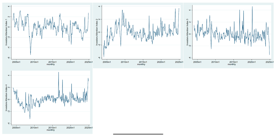
Furthermore, to examine that all the series are stationary, the Augmented Dickey Fuller (ADF) test was run (Appendix A). All the variables are significant except for hence by taking first difference it is converted into stationary () and is used in the index. The line graphs of each variables in Appendix B gives the graphical presentation of index variables. Through PCA analysis four indices are constructed mainly these indices have eigenvalues approximate equal to 1 or greater than 1. Please see screeplot of eigenvalues in Appendix C. The scoreplot and loadings of components are shown in Appendix D. The loadings are estimated and based on the loadings four indices are created, mainly because all the components explain 12% to 26% and cumulatively 73% of the variations. Then, Kaiser-Meyer-Olkin (KMO) is run to examine the sampling adequacy. The linearity assumption of OLS regression is examined through scatter plot (see Appendix F). The OLS regression and it’s four assumptions (heteroscedasticity, autocorrelation, multicollinearity, and normality) empirical tests results are shown in Appendix G. As some of the assumptions not fulfilled, hence we have to use GLS regression. Based on the attention index, the forecasting regression equation 8 mentioned below is considered for the current research.
(8)
where is KSE-100 index excess return, denotes the slope of regression on the attention proxyat time , and is the noise term. To estimate the model above, the OLS regression is used in line with the literature to examine the impact of investor attention on excess stock market returns, also known as market risk premium.
4. Results and Discussions
4.1. Descriptive and Correlation Analysis
This study uses monthly data comprising 252 observations (months) as shown in Table 2.
The mean of Nearness to KSE-100 Index 52-Week High () is 0.861 with SD of 0.115, a minimum value of 0.395, maximum of 1, p1 is 0.552, and p99 is 1; skewness is -0.974, showing negatively skewed data, kurtosis is 3.628, which is greater than 3, meaning the data is leptokurtic. Nearness to KSE-100 Index Historical High () has a mean of 0.241, SD of 0.164, minimum and maximum are 0.041 and 1, p1 is 0.044, p99 is 0.772, positively skewed with 1.061, and 4.872 is kurtosis, showing leptokurtic data. The mean of Abnormal Trading Volume () is 0.996, SD is 0.365, the minimum value is 0.004, the maximum value is 2.361, p1 is 0.212, and p99 is 2.013. The variable has positively skewed data with skewness of 0.58 and kurtosis of 3.707, that is greater than 3, representing leptokurtic data.
The mean value of Google Search Volume () is 10.442, with an SD of 2.862, a minimum search of 1.373, and a maximum of 19.529. It has p1 of 2.41 and p99 of 18.049, along with the skewness of -.22 and kurtosis of 3.967, indicating the data is leptokurtic. Extreme Returns () represents extreme returns with a 0.080 mean value and 0.021 SD, minimum extreme returns of 0.001 and 0.233 with maximum extreme returns, p1 is 0.041, p99 is 0.157, skewness of 2.585, and kurtosis of 18.498, showing leptokurtic data series. The mean value of Past Returns () is 0.238 with SD of 0.346, -0.56 of minimum past returns and 1.397 maximum returns with p1 of -0.529 and p99 of 1.19 skewness of 0.269 and kurtosis of 2.965 show data is platykurtic. Equity Mutual Funds Inflow () mean value is 2,404.89, SD of 659.002, a minimum of 1258.84, and a maximum of 4666.71, p1 is 1306.07, and p99 is 4163.15 with skewness of 1.257 and kurtosis of 4.088. descriptive statistics show that the index has produced average -0.088 excess returns along with an SD of 0.081. The index produced a minimum excess return of -0.483, and a maximum of 0.167, during the period of study. The lowest percentile p1 is -0.297, and the largest percentile p99 is 0.107, with -0.504 skewness and kurtosis of 5.309 showing leptokurtic behavior.
4.2. Attention Index Construction Through PCA and Its Impact on Stock Market Returns of KSE-100 Index
For the construction of an attention index it is important to have relationship among the variables. Table 3 showed a negative and weak to moderate correlation of , andof -0.288, and -0.176 with the dependent variable. The variables ,, ,, andhave positive but weak to moderate correlations of 0.387, 0.566, 0.112, 0.271, and 0.163 with . The results showed that the variables are significant and do not have the problem of multicollinearity.
Table 4 shows eigenvalues for each component. As per the rules of PCA, if eigenvalues are greater than and/or equal to one (eigenvalues >= 1), such components should be included for further analysis. The eigenvalue suggested by (Cattell, 1966) stated that four components should be retained for factor analysis of this research. Eigenvalues for Comp1 is 1.831, Comp2 is 1.334, Comp3 is 1.030 and Comp4 is 0.924. The eigenvalues show the total variance each factor accounts for (Mooi et al, 2018). The proportion of Comp1 explains 26.2%, Comp2 explains 19.1%, Comp3 explains 14.7%, and Comp4 explains 13.2% of the overall variance. Based on the PCA results, four attention indices are predicted; Comp1 is the first attention index denoted by , Comp2 is the second index , Comp 3 is the third index , and Comp 4 is the fourth index .
The eigenvectors of each variable of each component of PCA are mentioned in Table 5. According to Mooi et al. (2018) PCA eigenvectors comprised of factor weights that help in getting the maximum variance until significant part of the variables’ variance is explained. The unexplained column in Table 5 shows that unexplained variance of four components.
The aggregate attention index is constructed using a combination of factor weights of the individual attention proxies available in Table 5:
(7)
(8)
(9)
(10)
The coefficients of Eigenvalues of each variable in each component are provided in Table 6. In order to identify which factors, load the most in the respective index, the coefficients below 0.3 are removed. For graphical representation of Table 6.
According to the results of Table 6, the following proxies contribute higher to the indices , , , and . Hence, the major contributions are of these factors:
(11)
(12)
(13)
(14)
The attention indices loadings are estimated and the indices are constructed based on the loadings. The Kaiser–Meyer–Olkin (KMO) results are used to analyze the adequacy of samples because the correlations and partial correlations between variables are compared by KMO value in Table 7.
The KMO value for this study is 0.5248, which indicates a middling sample and highlights that correlations are high compared to partial correlations. We examine the data pattern and stationarity of , , , and through line graphs and ADF tests (Appendix E). All the indices are stationary. The Descriptive statistics of the aforementioned variables are shown in Table 8. The mean value of all the four indices is equals to zero and standard deviation (SD) is in the range of 1.057 and 1.245 indicating higher volatility in , the main index explaining 26.2% variations (see Table 4). descriptive statistics shows the minimum value is -5.372, maximum is 3.848, p1 is -3.848, maximum is 2.818, skewness is -0.368 and kurtosis is 4.478, showing non-normal and leptokurtic pattern. The second index is which explains the 19.1% variations (see Table 4) has SD of 1.157, minimum is -2.595, maximum is 3.054, p1 is -1.944, p99 is 2.603, skewness is 0.584, and kurtosis is 2.605. These statistics show that it has relatively less variations as compared to the first index. The third index explains 14.7% variations (see Table 4), have comparatively lower SD of 1.152, minimum of -4.456 and maximum of 4.084 along with p1 of -3.487, p99 of 2.655, skewness of -0.226, and kurtosis of 4.583. Like , this index also has negative skewness and leptokurtic curve. The fourth and the last index is explains 13.2% total variance (see Table 4), has lowest SD of 1.057, minimum of -3.32, highest maximum of 6.101, p1 of -1.822, p99 of 3.534, skewness of 1.685, and kurtosis of 9.377 showing positively skewed and leptokurtic curve. All these four indices cumulatively explain the total variance of 73.1% (see Table 4).
Table 9 shows the the correlation of , , andwith . The results shows positive moderate and significant relation among all the indices except for shows negative correlation
Once the components were analyzed, we regressed each of the attention indices with the to investigate whether investors’ attention index developed using PCA influence index returns or not. The GLS regression results are presented in Table 10:
Table 10 illustrates the empirical results examining the impact of each attention index on the KSE 100 Index excess returns while keeping all other factors constant. The probability values of F-test of all models are significant at 1% significance level. Theof model 1 is 0.167, model 2 is 0.080, model 3 is 0.430, and of model 4 is 0.080 explaining 16.7%, 8%, 43%, and 8% of the variations in the returns. In model 1 is regressed on , with of 0.029 and p-value of 0.000 showing positive and significant impact on . The model 2 shows the results of on having of 0.022 and significant at 1% significance level (p-value = 0.000) indicating increase in have positive and significant impact on returns. Among all the four models, model 3 (regressed on ) has the better explanatory power along with negative but significant of -0.051 and p-value of 0.000 and 1% significance level. In model 4, the impact of is examined, the results showed of 0.026 is positive and significant at 1% significance level, meaning an increase in would increase market returns. Concisely, models 1, 2 and 4 showed that the more the investors’ attention, the better the KSE 100 Index performs, along with higher returns. However, model 3 showed the negative impact on the index returns. Furthermore, the results support Prospect Theory (Kahneman & Tversky, 1979), which helps to explain the impact of attention on stock returns. The investors do take investment decisions or pay attention to the stocks that have a significant impact on the stock returns based on their psychology and available information.
From all seven proxies, the results of showed four variables that significantly contribute to the attention index along with an of 43%. It comprises,, , and proxies, as shown in Table 6. Thus, other factors that affect the attention index can explain the remaining 57% of the variability in returns. As Chen et al. (2022) mentioned that the sign of beta coefficients can be positive or negative or inconclusive. This study results also support their proposition as the beta coefficients ofis negative and of , and are positive, showing both negative and positive, and significant impact of attention indices on excess stock returns. Furthermore, the results of , , and supports Barber and Odean (2008) and Peng and Xiong (2006) findings that individual investors are more attentive to attention grabbing stocks and are the net buyers which simultaneously leads to positive pressure on stock prices but lower future stock returns (Chen et al., 2022).
5. Discussion
The current findings support Peng and Xiong (2006), Barber and Odean (2008), and Chen et al. (2022) studies that investor attention is a crucial factor in the dynamics of stock markets. The same is true in the Pakistan stock market. The aggregate attention index used in this study performs well, as it has taken the relevant and recent information by incorporating proxies that help in measuring the true attention of investors on the Pakistan Stock market. The finding show that higher investors’ attention leads to active trading in KSE-100 index and results in higher returns. However, the negative attention index means the lower investors’ attention leads to poor index performance. The changes in investors’ attention may be influence by some other factors including expansionary and contractionary monetary and fiscal policies along with different phases on business cycles. The empirical findings also support previous literature and underpinned theories.
Some of the previous studies used different proxies or factors, such as Hirshleifer et al. (2013) studies Analyst Coverage, and the results showed that the stock returns tend to be high for those firms that are efficient in research and development, and because of increasing expected earnings per share. Lou (2014) used Advertising Spending as a proxy, and the results showed that an increase in advertising spending leads to a simultaneous increase in stock price, followed by a complete return reversal. Chemmanur and Yan's (2019) findings were that advertising in the US stock market attracts investors’ attention to the firm’s stocks and affects future returns. Media coverage was also considered an attention measure (Hillert & Ungeheuer, 2015; Zou et al., 2019). Different researchers have already studied the factors above, but in Pakistan, the major limitation was the unavailability of data on these factors. In addition, macroeconomic factors and monetary policy also affect investors' attention. Therefore, Choi and Choi (2019) studied the US equity market and identified a negative and significant relationship between investor attention and abnormal trading volume at the market level. Their study concluded that when investors paid high attention to the stocks, the trading volume of such stocks increased suddenly and unexpectedly on that day. Thus, due to short-sell constraints, high investor attention results in low future returns through active trading. Aboody et al. (2010) took top percentile stocks that were ranked based on prior 12-month price performance for the 1971 through 2005 period and showed that strong past returns tend to attract individual investors’ attention, particularly before earnings announcements.
In this study, the attention index proxies have an impact on excess returns. The proximity to the 52-historical high in and has a negative influence on excess returns. The results support Li and Yu (2012), who found that heightened attention to this factor adversely affects future stock returns. Chang et al. (2018) investigated the impact of a historically high ratio on stock index returns of G7 countries. The authors found an inverse correlation between the historical high and the stock returns, attributing this to the significant gap. Our findings also support the results as historical high has a negative relationship with KSE 100 Index excess returns. Google Search Volume Index (GSVI) was used as a proxy measure for investor attention as the authors considered it a reliable proxy (Aouadi et al., 2013; Ding & Hou, 2015; Yao et al., 2017). In this study, Google Search Volume Index has a positive relationship as the more investors are interested in a stock, they give more attention to the stock and search for the company's technical and fundamental analysis using Google.
The findings are consistent with the literature. Chen et al. (2022) also concluded that the index had a negative but significant impact on future stock returns of the NASDAQ market. The negative coefficient is consistent with the literature review on investors’ attention index. Yuan (2015) found that market-wise events that grasped the attention of investors led to a decrease in stock returns in the future.
From the study, market participants could be able to identify key strategic directions that could assist them in understanding market conditions. In addition, appropriate investment decisions could be of considerable benefit and a competitive advantage in the market. It would help academic scholars in behavioral finance and open a new perspective. Besides this, the researcher would look at the signals that affect the performance of the KSE-100 index, effectively managing their portfolios and risk.
6. Conclusions, Limitations, Implications, and Recommendations
This paper aimed to illuminate the critical and growing phenomenon of investor attention in the Pakistani stock market by systematically analyzing attention proxies affecting stock market returns. For the first time, , , , , , and These proxies were used to construct the investor attention index through the PCA approach, which is renowned for its market prediction capabilities. The findings reveal that , and have positive and significant impact on KSE-100 Index excess returns. However, has a negative but significant impact on the index excess returns. The results are consistent with Chen et al. (2022) and Chen (2017).
This study highlights the importance of investor attention in Pakistan’s equity market and its substantial role in behavioral finance. Two primary economic sources were identified: first, lower investor attention leads to higher future uncertainty, prompting investors to demand higher returns as compensation for increased risk, resulting in higher stock returns. Second, heightened investor attention can lead to a surge in trading volume due to active trading and short-sell constraints, ultimately leading to lower future returns. Furthermore, this research underscores two significant points: investor attention substantially influences the aggregate stock market statistically and economically, and individual attention measures understate the true predictive power of investor attention in Pakistan’s stock market when analyzed through PCA. In conclusion, this study has provided valuable insights into examining the investor attention in Pakistan’s stock market, paving the way for future research to build upon these findings and explore new dimensions in behavioral finance.
However, this research encountered several limitations, including factors such as fluctuations in advertising expenditures, media coverage, analyst coverage, and other economic and firm-specific variables are excluded because of data unavailability in Pakistan. The study period was limited from January 1, 2004, to December 31, 2024 due to the availability of Google Search Volume data from 2004. The analysis was also confined to the KSE-100 Index, assuming it represents the Pakistani stock market. Additionally, due to time constraints and the COVID-19 pandemic, the research was limited to market-based variables and in-sample analysis, with data analysis conducted solely using STATA.
In addition, we have considered bivariate regression, hence resulting in lower . For better explanatory power, multivariate regression analysis can be done, including macroeconomic variables and other proxies based on the availability of data. Furthermore, it would be valuable to analyze the impact on other indices and conduct comparative analyses.
The major implications of this study are a need for more financial literacy and an understanding of investment strategies for earning higher returns. Policymakers can develop and implement transparent policies and procedures to increase effective trading in the stock market. Furthermore, they can offer incentives to investors so that more investors can participate in equity trading, which would help in creating market liquidity, make it transparent, and motivate both national and international investors to participate. The policymakers can also plan a capital gain tax, which would increase their revenues and would not hurt investors’ sentiments, which is crucial for sustainable growth. Furthermore, learning about the investors’ attention pattern would help in reducing the chances of creating a bubble, which would lead to a financial crisis in the future, and eliminate speculations. Individual investors can also increase returns by understanding the market sentiments and information. Mutual fund managers and practitioners can design portfolios based on individual investors’ behavior and risk appetite to maximize future returns. Scholars and academicians can conduct further research studies to understand investors’ attention behavior in different market scenarios and contribute to strengthening knowledge of behavioral finance.
In this study, a few recommendations are given to researchers and financial institutions who are highly inspired to conduct research, especially in this domain. The authors can consider economic variables for constructing an investor attention index and investigate their impact on returns. The authors can use firm-specific variables such as dividend-to-price ratio, earnings-to-price ratio, dividend payout ratio, book-to-market ratio, and the like. The researchers may consider specific industries where investor attention is analyzed, including health, manufacturing, energy, telecommunication, and more.
Author Contributions
“Conceptualization, S.P. and H.Z.; methodology, R.M. and S.A.; software, H.Z. and E.T.; validation, S.P., R.M.; formal analysis, S.A.; investigation, E.T.; resources, S.A.; data curation, H.Z.; writing—original draft preparation, S.P.; writing—review and editing, S.A.; visualization, E.T.; supervision, H.Z.; project administration, R.M.; funding acquisition, E.T. All authors have read and agreed to the published version of the manuscript.”.
Funding
The study does not receive any external funding. This manuscript has been submitted by prof. Eleftherios Thalassinos who is guest editor of special issue of JRFM and it is complementary publication.
Data Availability Statement
Upon request from the corresponding author.
Conflicts of Interest
The authors declare no conflict of interest.
Appendix A
Augmented Dickey Fuller Test Results of Index Variables
| Variable | ADF P-value |
| 0.0000 | |
| 1.0000 | |
| 0.0000 | |
| 0.0000 | |
| 0.0207 | |
| 0.0000 | |
| 0.0140 | |
| 0.0138 | |
| 0.0000 |
Appendix B. Graphical Analysis
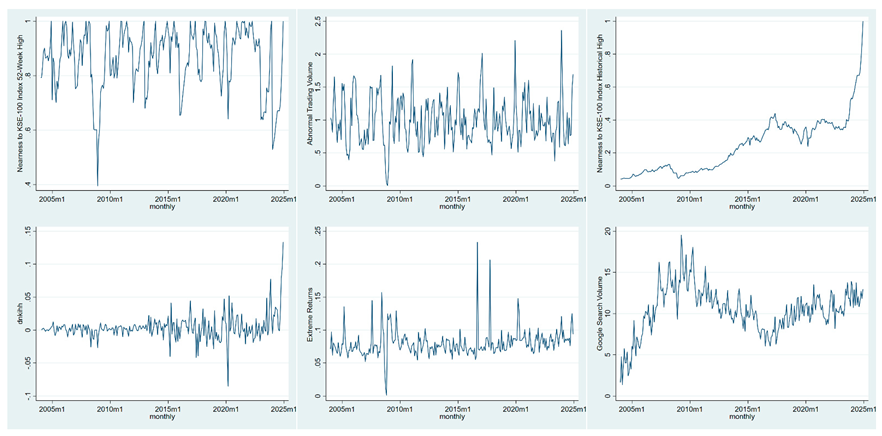
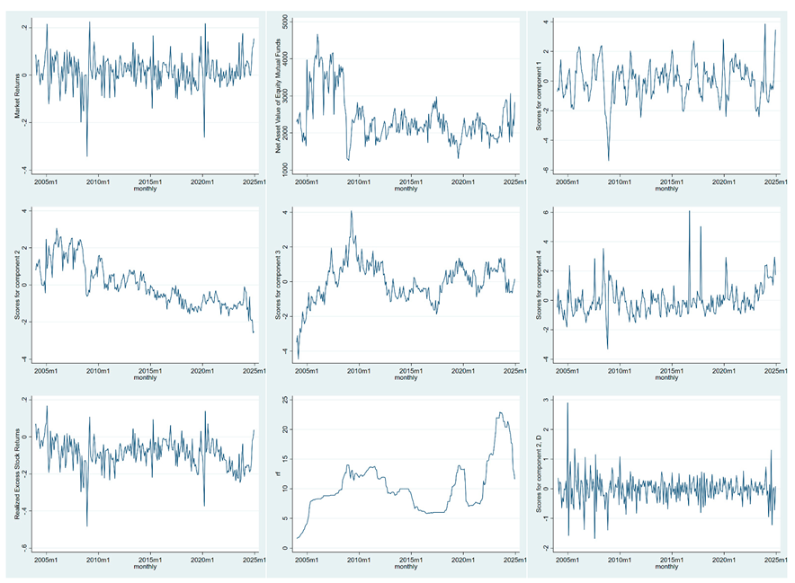
Appendix C. Screeplot
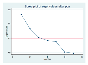
Appendix D. Score and Loading Plots
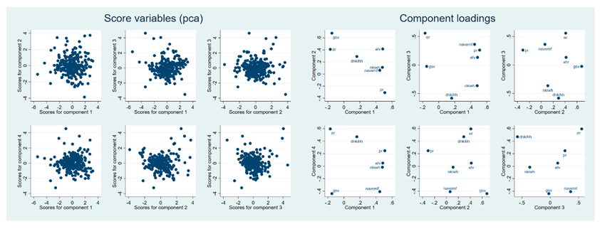
Appendix E. Indices Line Graphs and Augmented Dickey Fuller Test Results of Indices
Appendix F. Scatterplots-Linearity
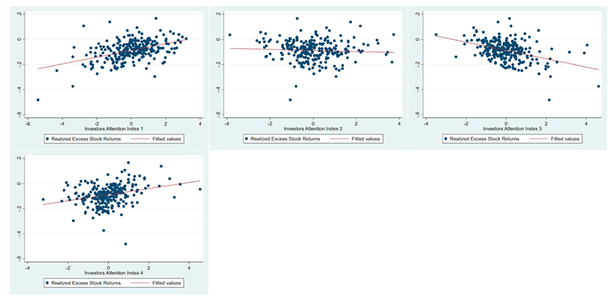
Appendix G. OLS Regression Estimation and Assumptions Results
| OLS Regression Estimation and Assumptions Results | |||||||||||||
| Regress | Dependent variable | Investor Attention Index | Beta coefficients | p-value | Alpha coefficients | p-value | F-stats | F-Test p-value | Adj R2 | Durbin-Watson | Jarque Bera | Hettest | VIF |
| 1 | 0.027 | 0.000 | -0.088 | 0.000 | 63.75 | 0.000 | 0.200 | 1.424 | 0.000 | 0.000 | 1.000 | ||
| 2 | 0.026 | 0.040 | -0.089 | 0.000 | 20.85 | 0.000 | 0.074 | 1.304 | 0.000 | 0.087 | 1.000 | ||
| 3 | -0.033 | 0.000 | -0.088 | 0.000 | 51.72 | 0.000 | 0.169 | 0.916 | 0.000 | 0.000 | 1.000 | ||
| 4 | 0.024 | 0.000 | -0.088 | 0.000 | 22.53 | 0.000 | 0.079 | 1.29 | 0.000 | 0.207 | 1.000 | ||
References
- Abideen, Z. U. , Ahmed, Z., Qiu, H., & Zhao, Y. (2023). Do behavioral biases affect investors’ investment decision making? Evidence from the Pakistani equity market. Risks, 11(6), 109. [CrossRef]
- Aboody, D. , Lehavy, R. ( 15(2), 317–344. [CrossRef]
- Ahmad, N. , & Ramzan, M. (2016). Stock Market Volatility and Macroeconomic Factor Volatility. International Journal of Research in Business Studies and Management, 3(7).
- Aouadi, A. , Arouri, M., & Teulon, F. (2013). Investor Attention and Stock Market Activity: Evidence from France. Economic Modelling, 35, 674–681. [CrossRef]
- Baker, M. , & Wurgler, J. (2006). Investor sentiment and the cross-section of stock returns. The Journal of Finance, 61(4), 1645-1680. [CrossRef]
- Banerjee, A. V. (1992). A simple model of herd behavior. The quarterly journal of economics, 107(3), 797-817. [CrossRef]
- Barber, B. M. , & Odean, T. (2008). All that Glitters: The Effect of Attention and News on the Buying Behavior of Individual and Institutional Investors. Review of Financial Studies, 21(2), 785–818. [CrossRef]
- Barberis, N. , & Huang, M. ( 56(4), 1247–1292. [CrossRef]
- Bikhchandani, S. , Hirshleifer, D. ( 100(5), 992–1026.
- Cattell, R. B. (1966). The scree test for the number of factors. Multivariate behavioral research, 1(2), 245-276. [CrossRef]
- Chang, S. L. , Chien, C. Y., Lee, H. C., & Lin, C. (2018). Historical High and Stock Index Returns: Application of the Regression Kink Model. Journal of International Financial Markets, Institutions and Money, 52, 48–63. [CrossRef]
- Chemmanur, T. J. , & Yan, A. (2019). Advertising, Attention, and Stock Returns. Quarterly Journal of Finance, 9(3). [CrossRef]
- Chen, T. (2017). Investor Attention and Global Stock Returns. Journal of Behavioral Finance, 18(3), 358-372. [CrossRef]
- Chen J, Tang G, Yao J, Zhou G. ( 57(2), 455–484. [CrossRef]
- Choi, S. , & Choi, W. Y. (2019). Effects of Limited Attention on Investors’ Trading Behavior: Evidence from Online Ranking Data. Pacific Basin Finance Journal, 56(18), 273–289. 20 June. [CrossRef]
- Chu, G. , Goodell, J. W., Shen, D., & Zhang, Y. (2022). Machine learning to establish proxies for investor attention: evidence of improved stock-return prediction. Annals of Operations Research, 318(1), 103-128. [CrossRef]
- Da, Z. , Engelberg, J. ( 66(5), 1461–1499.
- Ding, R. , & Hou, W. ( 37, 12–26. [CrossRef]
- Düz Tan, S. , & Taş, O. (2019). Investor Attention and Stock Returns: Evidence from Borsa Istanbul. Borsa Istanbul Review, 19(2), 106–116. [CrossRef]
- Fama, E. F. (1970). Efficient capital markets. Journal of Finance, 25(2), 383-417.
- Ghani, M. , Guo, Q., Ma, F., & Li, T. (2022). Forecasting Pakistan Stock Market Volatility: Evidence from Economic Variables and the Uncertainty Index. International Review of Economics & Finance, 80, 1180–1189.
- Gill, R. K. , & Bajwa, R. ( 8(3), 1–14.
- He, M. , Zhang, Y., Wen, D., & Wang, Y. (2021). Forecasting crude oil prices: A scaled PCA approach. Energy Economics, 97, 105189. [CrossRef]
- Hillert, A. , & Ungeheuer, M. (2015). Ninety Years of Media Coverage and the Cross-Section of Stock Returns. SSRN Electronic Journal, March, 1–2. [CrossRef]
- Hirshleifer, D. , Hsu, P. ( 107(3), 632–654. [CrossRef]
- Hirshleifer, D. , & Teoh, S. H. (2003). Limited Attention, Information Disclosure, and Financial Reporting. Journal of Accounting and Economics, 36(1-3 SPEC. ISS.), 337–386. [CrossRef]
- Hong, H. , & Stein, J. C. ( 54(6), 2143–2184. [CrossRef]
- Huang, L. , & Liu, H. ( 62(4), 1999–2040. [CrossRef]
- Ibikunle, G. , McGroarty, F., & Rzayev, K. (2020). More Heat Than Light: Investor Attention and Bitcoin Price Discovery. International Review of Financial Analysis, 69(January), 101459. [CrossRef]
- Joyo, A. S. , & Lefen, L. (2019). Stock Market Integration of Pakistan with its Trading Partners: A Multivariate DCC-GARCH Model Approach. Sustainability, 11(2), 303.
- Kahneman, D. (1973). Attention and Effort. (vol. 1063, pp. 218-226). Prentice-Hall.
- Kahneman, D. , & Tversky, A. (1979). Prospect theory: An analysis of decision under risk. Econometrica, 47(2), 263–292.
- Li, J. , & Yu, J. ( 104(2), 401–419. [CrossRef]
- Lou, D. (2014). Attracting investor attention through advertising. Review of Financial Studies, 27(6), 1797–1829. [CrossRef]
- Ludvigson, S. C. , & Ng, S. (2007). The empirical risk–return relation: A factor analysis approach. Journal of financial economics, 83(1), 171-222. [CrossRef]
- Mangi, F. (2016). Pakistan Stocks Jump Most in a Year as MSCI Seen Luring Cash, Bloomberg, available at: https://www.bloomberg.com/news/articles/2016-06-15/pakistani-stocks-jump-most-this-year-after-upgrade-from-msci.
- Merton, R. C. (1987). A Simple Model of Capital Market Equilibrium with Incomplete Information.
- Miller, E. M. (1977). Risk, uncertainty, and divergence of opinion. The Journal of finance, 32(4), 1151-1168. [CrossRef]
- Mooi, E. , Sarstedt, M., Mooi-Reci, I., Mooi, E., Sarstedt, M., & Mooi-Reci, I. (2018). Principal component and factor analysis. Market research: The process, data, and methods using Stata, 265-311. [CrossRef]
- Neely, C. J. , Rapach, D. E., Tu, J., & Zhou, G. (2014). Forecasting the equity risk premium: the role of technical indicators. Management science, 60(7), 1772-1791. [CrossRef]
- Pashler, H. , Johnston, J. ( 52(1), 629–651. [CrossRef] [PubMed]
- Peng, L. , & Xiong, W. ( 80(3), 563–602. [CrossRef]
- Resta, M. (2016). Enhancing self-organizing map capabilities with graph clustering: An application to financial markets. Intelligent Systems in Accounting, Finance and Management, 23(1-2), 21-46.
- Seasholes, M. S. , & Wu, G. ( 14(5), 590–610. [CrossRef]
- Shafique, A. , Ayub, U., & Zakaria, M. (2019). Don’t let the Greed catch you! Pleonexia rule applied to Pakistan Stock Exchange. Physica A: Statistical Mechanics and Its Applications, 524, 157-168. [CrossRef]
- Shah, S.Z.A. , Ahmad, M. and Mahmood, F. (2018). Heuristic biases in investment decision-making and perceived market efficiency: A survey at the Pakistan stock exchange. Qualitative Research in Financial Markets, Vol. 10 No. 1, pp. 85-110. [CrossRef]
- Simon, Herbert A., 1955a, “A Behavioral Model of Rational Choice”, Quarterly Journal of Economics, 69(1): 99–118. [CrossRef]
- Smales, L. A. (2021). Investor Attention and Global Market Returns During the COVID-19 crisis. International Review of Financial Analysis, 73(20), 101616. 20 June. [CrossRef]
- Song, Z. , Gong, X., Zhang, C., & Yu, C. (2023). Investor sentiment based on scaled PCA method: A powerful predictor of realized volatility in the Chinese stock market. International Review of Economics & Finance, 83, 528-545. [CrossRef]
- Subramaniam, S. , & Chakraborty, M. (2020). Investor Attention and Cryptocurrency Returns: Evidence from Quantile Causality Approach. Journal of Behavioral Finance, 21(1), 103–115. [CrossRef]
- Tversky, A. , & Kahneman, D. (1973). Availability: A heuristic for judging frequency and probability. Cognitive psychology, 5(2), 207-232. [CrossRef]
- Tversky, A. , & Kahneman, D. (1974). Judgment under Uncertainty: Heuristics and Biases: Biases in judgments reveal some heuristics of thinking under uncertainty. science, 185(4157), 1124-1131. [CrossRef]
- Tversky, A. , & Kahneman, D. (1992). Advances in prospect theory: Cumulative representation of uncertainty. Journal of Risk and uncertainty, 5, 297-323. [CrossRef]
- Wang, B. , Long, W., & Wei, X. (2018). Investor attention, market liquidity and stock return: A new perspective. Asian Economic and Financial Review, 8(3), 341. [CrossRef]
- Yahya, F. , Shaohua, Z., Abbas, U., & Waqas, M. (2021). COVID-19-induced Returns, Attention, Sentiments and Social Isolation: Evidence from Dynamic Panel Model. Global Business Review. [CrossRef]
- Yao, T. , Zhang, Y. J., & Ma, C. Q. (2017). How Does Investor Attention Affect International Crude Oil Prices? Applied Energy, 205(July), 336–344. [CrossRef]
- Yuan, Y. (2015). Market-wide Attention, Trading, and Stock Returns. Journal of Financial Economics, 116(3), 548–564. [CrossRef]
- Zada, H. , Maqsood, H., Ahmed, S., & Khan, M. Z. (2023). Information shocks, market returns and volatility: a comparative analysis of developed equity markets in Asia. SN Business & Economics, 3(1), 37.
- Zhang, W. , Shen, D. ( 33, 613–619. [CrossRef] [PubMed]
- Zou, L. , Cao, K. D., & Wang, Y. (2019). Media Coverage and the Cross-Section of Stock Returns: The Chinese Evidence. International Review of Finance, 19(4), 707–729. [CrossRef]
Figure 1.
LSEG data for the KSE-100 Index.
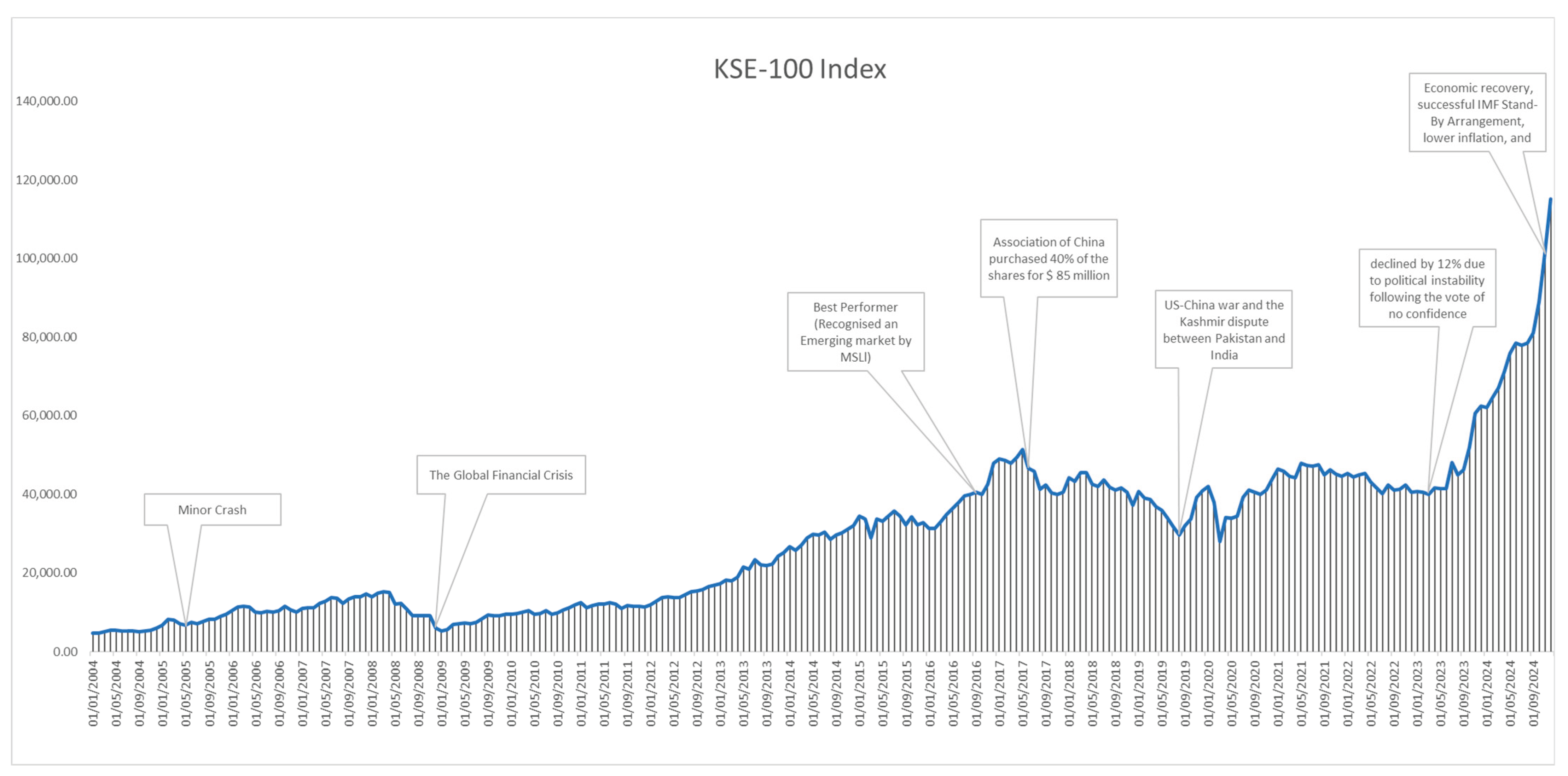

Table 1.
Definition and Operationalization of Variables.
| Variables | Symbol and Operationalization | Definition |
|---|---|---|
| Abnormal Trading Volume |
(1) |
In equation 1, is the equal-weighted abnormal trading volume () at time across all stocks. It is calculated as a ratio stock’s trading volume () at time to its average trading volume () over the previous year. According to Barber and Odean (2008), when abnormally heavy trading volumes are observed in the stock market, investors are more attracted to these shares than usual. Hence, it is a measure of the market-level attention index. |
| Extreme Returns | (2) | According to Barber and Odean (2008), investors notice extreme one-day returns, positive or negative, mostly when news about the company occurs. Hence, extreme returns play a significant role in measuring investors' attention. In equation 2, is ratio of extreme returns () at the end of each month to the average of extreme returns over the previous one year for each stock (). Hence, is the equal-weighted extreme returns at time across all stocks. |
| Past Returns | Aboody et al. (2010) highlighted those stocks with sharp past returns attract investors’ attention. Also, the company’s earnings announcements grab attention; hence, there is a need to include past returns proxy in the investors’ attention index. is the cumulative monthly returns for the past twelve months for each stock at time is calculated which is the equal weighted past return across all stocks. | |
| Nearness to the KSE-100 Index 52-week high | (3) | To empirically test psychological anchoring and limited investor attention, Li and Yu (2012) used Nearness to the Index 52 week high () and historical high proxies. Furthermore, the authors stated that helps in measuring the extent of under-reaction and in predicting the aggregate market returns. In equation 3, is the ratio of the current level of KSE-100 index () at end of month to its 52-week high () at month . |
| Nearness to the KSE-100 Index historical high | (4) | Li and Yu (2012) used Nearness to the KSE-100 Index historical high () specifically to examine when current price is far from the historical high price, it is the time when investors react to the bad news. The authors stated that the investors over react because there has been a series of bad news in the past, and prolonged news has negative impact on future market returns. In equation 4, is the ratio of the current KSE-100 index () at end of month to its historical high () at the end of month . The is the maximum index value of KSE-100 price index dataset from January 2004 to December 2024. |
| Google Search Volume | Da et al. (2011) proposed Google aggregate search frequency as a direct measure of investors’ attention. is the monthly aggregate search frequency of companies listed on KSE-100 Index from Google Trends using stock ticker. The data is available from January 2004 onwards. | |
| Equity Mutual Funds Inflow | denotes the net asset value of mutual funds inflow for each equity mutual fund , at the end of month . Like Chen et al. (2022), we computed the equal-weighted mutual funds inflow as proxy for market level. | |
| KSE 100 Index Returns | (5) | is the index returns, is the KSE-100 Index price at time and is the index price at time . |
| KSE 100 Index Excess Returns | (6) | is the KSE-100 Index excess market returns. It is the difference of and (three-month treasury bill rate) |
Table 2.
Descriptive Statistics of Investors’ Attention Proxies and KSE-100 Index Returns.
| Variables | Obs | Mean | SD | Min | Max | P1 | P99 | Skew | Kurt |
| 252 | .861 | .115 | .395 | 1 | .552 | 1 | -.974 | 3.628 | |
| 252 | .241 | .164 | .041 | 1 | .044 | .772 | 1.061 | 4.872 | |
| 252 | .996 | .365 | .004 | 2.361 | .212 | 2.013 | .58 | 3.707 | |
| 252 | 10.442 | 2.862 | 1.373 | 19.529 | 2.451 | 18.049 | -.22 | 3.967 | |
| 252 | .08 | .021 | .001 | .233 | .041 | .157 | 2.585 | 18.498 | |
| 252 | .238 | .346 | -.56 | 1.397 | -.529 | 1.19 | .269 | 2.965 | |
| 252 | 2404.885 | 659.002 | 1258.838 | 4666.711 | 1306.07 | 4163.147 | 1.257 | 4.088 | |
| 252 | -.088 | .081 | -.483 | .167 | -.297 | .107 | -.504 | 5.309 | |
| Note. Obs represents the number of observations, Mean is the average of investors’ index proxies, SD is the standard deviation, Min is the minimum value, Max is the maximum value in the data series, P1 is the first percentile, P99 is the ninety-ninth percentile, Skew represents skewness, and Kurt is kurtosis. The Table exhibits the descriptive statistics of key variables; (Nearness to KSE-100 Index 52-Week High), (Nearness to KSE-100 Index Historical High), (Abnormal Trading Volume), (Google Search Volume), (Extreme Returns), (Equity Mutual Funds Inflow), (Past Returns), and is the KSE 100 index excess returns. The data frequency is monthly, and the period is from January 2004 to December 2024. | |||||||||
Table 3.
Pairwise Correlation Matrix of Investors’ Attention Proxies.
| Variables | |||||||||
| 1.000 | |||||||||
| 0.387*** | 1.000 | ||||||||
| (0.000) | |||||||||
| 0.566*** | 0.123* | 1.000 | |||||||
| (0.000) | (0.052) | ||||||||
| 0.112* | 0.382*** | 0.107* | 1.000 | ||||||
| (0.077) | (0.000) | (0.091) | |||||||
| -0.288*** | -0.051 | 0.083 | 0.117* | 1.000 | |||||
| (0.000) | (0.420) | (0.188) | (0.065) | ||||||
| -0.176*** | -0.160** | -0.010 | 0.094 | 0.143** | 1.000 | ||||
| (0.005) | (0.011) | (0.877) | (0.137) | (0.023) | |||||
| 0.271*** | 0.187*** | 0.049 | 0.229*** | -0.335*** | -0.095 | 1.000 | |||
| (0.000) | (0.003) | (0.442) | (0.000) | (0.000) | (0.131) | ||||
| 0.163*** | 0.131** | 0.021 | 0.264*** | 0.043 | -0.089 | 0.327*** | 1.000 | ||
| (0.009) | (0.038) | (0.737) | (0.000) | (0.497) | (0.160) | (0.000) | |||
| Note. Table 3 illustrates the relationship between and seven attention index proxies.*** p<0.01, ** p<0.05, * p<0.1. | |||||||||
Table 4.
Principal Components Eigenvalue shows total variance explained by variables/factors.
| Component | Eigenvalue | Difference | Proportion | Cumulative |
| Comp1 | 1.831 | 0.498 | 0.262 | 0.262 |
| Comp2 | 1.334 | 0.303 | 0.191 | 0.452 |
| Comp3 | 1.030 | 0.107 | 0.147 | 0.599 |
| Comp4 | 0.924 | 0.040 | 0.132 | 0.731 |
| Comp5 | 0.883 | 0.363 | 0.126 | 0.857 |
| Comp6 | 0.520 | 0.042 | 0.074 | 0.932 |
| Comp7 | 0.478 | . | 0.068 | 1.000 |
Table 5.
Principal components (eigenvectors).
| Variable | Comp1 | Comp2 | Comp3 | Comp4 | Unexplained |
| 0.479 | 0.111 | -0.363 | -0.017 | 0.427 | |
| 0.161 | 0.291 | -0.582 | 0.470 | 0.287 | |
| 0.484 | 0.417 | 0.133 | 0.049 | 0.320 | |
| -0.170 | 0.411 | 0.559 | 0.596 | 0.073 | |
| 0.510 | -0.309 | 0.261 | 0.248 | 0.271 | |
| -0.150 | 0.679 | -0.025 | -0.440 | 0.164 | |
| 0.447 | 0.062 | 0.362 | -0.408 | 0.341 |
Table 6.
The Coefficients of Eigenvalues Results.
| Variable | Comp 1 (PCA1) | Comp 2 (PCA2) |
Comp 3 (PCA3) |
Comp 4 (PCA4) |
Unexplained | ||||||||
|
|
0.4792 0.4836 0.5095 0.4465 |
0.4168 0.4108 -0.3087 0.6793 |
-0.3634 -0.5816 0.5585 0.3621 |
0.4700 0.5958 -0.4397 -0.4084 |
0.4267 0.287 0.3195 0.0728 0.2707 0.1642 0.3407 |
||||||||
Table 7.
KMO Measure of Sampling Adequacy.
| Variable | KMO |
| 0.5595 0.6101 0.5368 0.4403 0.5400 0.4170 0.5693 |
|
| Overall | 0.5248 |
Table 8.
Descriptive Statistics.
| Variables | Obs | Mean | Std. Dev. | Min | Max | p1 | p99 | Skew. | Kurt. |
| 252 | 0 | 1.245 | -5.372 | 3.848 | -3.848 | 2.818 | -.368 | 4.478 | |
| 252 | 0 | 1.157 | -2.595 | 3.054 | -1.944 | 2.603 | .584 | 2.605 | |
| 252 | 0 | 1.152 | -4.456 | 4.084 | -3.487 | 2.655 | -.226 | 4.583 | |
| 252 | 0 | 1.057 | -3.32 | 6.101 | -1.822 | 3.534 | 1.685 | 9.377 |
Table 9.
Matrix of correlations.
| Variables | |||||
| 1.000 | |||||
| 0.451*** | 1.000 | ||||
| (0.000) | |||||
| 0.278*** | 0.019 | 1.000 | |||
| (0.000) | (0.760) | ||||
| -0.415*** | 0.000 | -0.019 | 1.000 | ||
| (0.000) | (1.000) | (0.765) | |||
| 0.288*** | 0.000 | 0.369*** | 0.000 | 1.000 | |
| (0.000) | (1.000) | (0.000) | (1.000) | ||
| *** p<0.01, ** p<0.05, * p<0.1 | |||||
Table 10.
Generalized Least Square Regression Results of each Attention Index.
| Variables | Coef. | St. Er. | t-value | p-value | R2 | F-test | Prob > F | Transformed DW |
| Model 1: | ||||||||
| 0.029 | 0.004 | 7.06 | 0.000*** | 0.167 | 49.85 | 0.000*** | 2.01 | |
| Constant | -0.088 | 0.006 | -14.27 | 0.000*** | ||||
| Model 2: | ||||||||
| 0.022 | 0.005 | 4.64 | 0.000*** | 0.080 | 21.55 | 0.000*** | 2.10 | |
| Constant | -0.089 | 0.007 | -12.80 | 0.000*** | ||||
| Model 3: | ||||||||
| -0.051 | 0.004 | -13.69 | 0.000*** | 0.430 | 187.33 | 0.000*** | 2.22 | |
| Constant | -0.090 | 0.010 | -9.24 | 0.000*** | ||||
| Model 4: | ||||||||
| 0.026 | 0.006 | 4.65 | 0.000*** | 0.080 | 21.67 | 0.000*** | 2.05 | |
| Constant | -0.088 | 0.007 | -12.38 | 0.000*** | ||||
| Table 10 presents the results of four GLS regressions examining the impact of , , , and attention indices on . *** and * shows significance at the 1% and 10% levels, respectively. DW denotes Durbin Watson. | ||||||||
Disclaimer/Publisher’s Note: The statements, opinions and data contained in all publications are solely those of the individual author(s) and contributor(s) and not of MDPI and/or the editor(s). MDPI and/or the editor(s) disclaim responsibility for any injury to people or property resulting from any ideas, methods, instructions or products referred to in the content. |
© 2025 by the authors. Licensee MDPI, Basel, Switzerland. This article is an open access article distributed under the terms and conditions of the Creative Commons Attribution (CC BY) license (http://creativecommons.org/licenses/by/4.0/).
Copyright: This open access article is published under a Creative Commons CC BY 4.0 license, which permit the free download, distribution, and reuse, provided that the author and preprint are cited in any reuse.


