On the Theory of Partial Difference Equations: From the Edge of Chaos to Quasichaos

1. Introduction to Partial Difference Equations

1.1. Motivation and Background

Modern biology is filled with complex systems, molecular networks, cellular structures, ecological populations, all of which are fundamentally discrete in nature. Molecules are countable, cells are spatially separated, and reproduction occurs in discrete generations. Even gene expression and mutation are not continuous flows, but sudden, often stochastic events.

Yet, most mathematical frameworks used to model biological or complex systems—particularly partial differential equations (PDE), are based on continuous variables and smooth approximations. While PDE have been powerful in physics and engineering, they often struggle to naturally express discrete interactions, abrupt transitions, or spatially distributed logical rules common in biological processes.

This discrepancy led me to ask: What if the true natural language of complex, emergent systems is not the continuous PDE, but the discrete counterpart, the Partial Difference Equation (P$\Delta$E)?

This paper emerges from that question. It is an attempt to lay down the theoretical foundation for Partial Difference Equations as a modeling framework for complex systems, especially those on the edge of chaos where local interactions lead to global emergence. I believe this formalism can provide a more faithful, elegant, and computationally grounded way of understanding biological dynamics.

1.2. Shift Operator

We define the shift operator $E^k$ acting on a function $x\left(t\right)$ as

$$E^{k}x:=x(t+k)$$

for any integer $k\in \mathbb{Z}$.

Examples.

$$\begin{array}{cc}\hfill Ex& =x(t+1)\hfill \\ \hfill E^{2}x& =x(t+2)\hfill \\ \hfill E^{-1}x& =x(t-1)\hfill \end{array}$$

1.3. Partial Shift Operator

Definition. Given a discrete scalar field $u(x_1,x_2,\dots ,x_n)$, the partial shift operator $E_{x_i}^{k_i}$ acts on u by shifting the i-th coordinate:

$$E_{x_i}^{k_i}u(x_1,\dots ,x_i,\dots ,x_n):=u(x_1,\dots ,x_i+k_i,\dots ,x_n)$$

Examples.

$$\begin{array}{cc}\hfill E_{t}u& =u(t+1,x,y,z)\hfill \\ \hfill E_x^{2}u& =u(t,x+2,y,z)\hfill \end{array}$$

In this paper, we will write all the Partial Difference Equations in terms of Shift Operators.

1.4. Ordinary Difference Equations

Definition 1

(Ordinary Difference Equation of Order k). An ordinary difference equation of order kis an equation involving a single-variable function $x:\mathbb{Z}\to \mathbb{C}$, expressed in terms of shift operators:

$$F(E^{n}x,E^{n-1}x,\dots ,Ex,x,E^{-1}x,\dots ,E^{-m}x,t)=0,$$

where $E^{i}x:=x(t+i)$, $n,m\in {\mathbb{Z}}^{+}$, $k=m+n$ is the total order, and F is a (possibly nonlinear) function.

Definition 2

(Definition: Linear Ordinary Difference Equation of Order k). A linear ordinary difference equation of order k is an equation of the form:

$$a_n\left(t\right)E^{n}x\left(t\right)+a_{n-1}\left(t\right)E^{n-1}x\left(t\right)+\cdots +a_0\left(t\right)x\left(t\right)+a_{-1}\left(t\right)E^{-1}x\left(t\right)+\cdots +a_{-m}\left(t\right)E^{-m}x\left(t\right)=g\left(t\right),$$

where:

• $x\left(t\right)$ is the unknown function defined on $\mathbb{Z}$,
• $E^{j}x\left(t\right):=x(t+j)$ is the shift operator,
• $a_j\left(t\right)$ are known coefficient functions,
• $g\left(t\right)$ is the known input or forcing term,
• $m,n\in \mathbb{N}$ and $k=m+n$ is the total order.

1.5. Partial Difference Equation

Definition 3

(General Partial Difference Equation). Let $u:{\mathbb{Z}}^n\to \mathbb{R}$ (or $\mathbb{C}$) be a scalar function defined on the discrete lattice. A partial difference equation (P$\Delta$E) is an equation of the form:

$$F\left({\left\{E_{x_1}^{k_1}{E}_{x_2}^{k_2}\cdots E_{x_n}^{k_n}u\right\}}_{(k_1,k_2,\dots ,k_n)\in S}\right)=0,$$

where:

• F is a given function, which may be linear or nonlinear;
• $E_{x_i}$ denotes the shift operator in the $x_i$-th direction, defined by

  $$E_{x_i}^{k_i}u=u(x_1,x_2,\dots ,x_i+k_i,\dots ,x_n);$$
• $S\subset {\mathbb{Z}}^n$ is a finite index set determining the set of applied shifts.

1.6. The Order of a Partial Difference Equation

We propose two types of order to classify the structure of partial difference equations: structural order and absolute order.

Definition 4

(Structural Order of Partial Difference Equation). Let $u=u(x_1,x_2,\cdots ,x_n)$ be a scalar function defined on a discrete lattice. A partial difference equation is of the form

$$F\left({\left\{E_{x_1}^{k_1}{E}_{x_2}^{k_2}\dots E_{x_n}^{k_n}u\right\}}_{(k_1,k_2,\dots ,k_n)\in S}\right)=0,$$

where $S\subset {\mathbb{Z}}^n$ is a finite index set of shifts.

For each variable $x_i$, define

$$ord\left(x_i\right)=max\left(k_i\right)-min\left(k_i\right),$$

where the maximum and minimum are taken over all values of $k_i$ appearing in S.

Then, the  structural order of the equation is defined as

$$max\left(ord\left(x_1\right),ord\left(x_2\right),\dots ,ord\left(x_n\right)\right).$$

Definition 5

(Absolute Order of Partial Difference Equation). Let $u=u(x_1,x_2,\cdots ,x_n)$ and consider a partial difference equation of the form

$$F\left({\left\{E_{x_1}^{k_1}{E}_{x_2}^{k_2}\dots E_{x_n}^{k_n}u\right\}}_{(k_1,k_2,\dots ,k_n)\in S}\right)=0,$$

where $S\subset {\mathbb{Z}}^n$ is a finite index set.

If for all $(k_1,\cdots ,k_n)\in S$, the sum

$$|k_1|+|k_2|+\dots +|k_n|\le k,$$

then the equation is said to have  absolute order  k.

In addition:

• A shift operator $E_x^n$ is said to be of order $\left|n\right|$.
• A mixed shift operator $E_{x_1}^{k_1}{E}_{x_2}^{k_2}\cdots E_{x_n}^{k_n}$ is said to be of order $|k_1|+|k_2|+\dots +|k_n|$.

1.7. Comparison with Ordinary Difference Equations

The essential difference lies in the function domain and structure:

• Ordinary Difference Equation (O$\Delta$E): Involves a single-variable function $x:\mathbb{Z}\to \mathbb{C}$, typically evolving along a one-dimensional time axis.
• Partial Difference Equation (P$\Delta$E): Involves a multi-variable function $u:{\mathbb{Z}}^n\to \mathbb{C}$, evolving over a multi-dimensional discrete lattice.
• P$\Delta$E equations utilize partial shift operators, such as $E_{x_i}$, acting independently on each coordinate axis, introducing more geometric and structural complexity.

1.8. Comparison with Partial Differential Equations

Partial difference equations can also be viewed as the discrete analogues of partial differential equations. Key distinctions include:

• Partial Differential Equations (PDE): Defined over continuous space-time domains. Dynamics are governed by partial derivatives, such as ${\displaystyle \frac{\partial u}{\partial x}}$ or ${\displaystyle \frac{{\partial }^{2}u}{\partial t^2}}$.
• Partial Difference Equations (P$\Delta$Es): Defined over discrete lattice domains, where partial derivatives are replaced by partial difference operators or partial shift operators, e.g. $E_{x_i}u=u(\dots ,x_i+1,\dots )$.
• P$\Delta$E capture the dynamics of discrete systems such as cellular automata, lattice models, or numerical schemes, and often exhibit different phenomena such as intrinsic stochasticity or discrete chaos.

1.9. Why P$\Delta$E Are Natural for Complex Systems

Many well-known complex systems, such as Conway’s Game of Life, the Abelian Sandpile Model, and the Forest Fire Model, they are defined on discrete spatial grids and evolve in discrete time steps. Despite their fame and frequent analysis, these systems are often described in algorithmic or simulation-based language, rather than formal mathematical equations.

Upon close observation, it becomes clear that all these models operate within a common framework: local update rules on spatiotemporal lattices. Their behavior is governed by local interactions and recursive update functions, which is precisely the structure captured by Partial Difference Equations (P$\Delta$Es).

This realization led me to propose a shift in formalism: Instead of interpreting such systems as informal cellular automata or approximations to PDEs, we should describe them explicitly as nonlinear PΔEs. Doing so allows us to apply analytical tools from dynamical systems theory, discrete calculus, and field theory, opening the door to a unified mathematical treatment of complexity across scales.

In this view, P$\Delta$Es are not only suitable but natural for modeling self organization, emergent behaviour, and dynamical patterns in complex systems.

1.10. Classification and Examples

Partial Difference Equations (P$\Delta$Es) can be categorized along several axes, including linearity, time-dependence, and dimensionality. Below are some common types:

1.

Linear P$\Delta$E: A P$\Delta$E is said to be linear if it is linear in u and all its shifted terms. For example:

$$E_{t}u={\displaystyle \frac{1}{2}}(E_x^{-1}u+E_{x}u)$$

This equation represents a discrete diffusion process, where the future state is the average of neighboring spatial values.

2.

Nonlinear P$\Delta$E: Nonlinear P$\Delta$Es contain nonlinear terms involving u or its shifts. For example:

$$E_{t}u=u+sin(E_x^{-1}u-E_{x}u)$$

Such systems can exhibit complex behavior, including chaos and pattern formation.

3.

Autonomous P$\Delta$E: If the evolution rule is independent of the explicit time step t, the equation is said to be autonomous:

$$E_{t}u=F\left({\left\{E_x^{k}u\right\}}_{k\in N}\right)$$

These are time-invariant systems and useful for studying equilibrium dynamics.

4.

Non-Autonomous P$\Delta$E: If the update rule explicitly depends on t or x, the system is non-autonomous:

$$E_{t}u=F(t,x,{\left\{E_x^{k}u\right\}}_{k\in N})$$

These equations are useful for modeling time-varying or spatially heterogeneous environments.

5.

System of P$\Delta$E: A coupled system of multiple interacting fields:

$$\left\{\begin{array}{c}{E}_{t}u=f(u,E_{x}u,E_x^{-1}u,v,E_{x}v,E_x^{-1}v)\hfill \\ E_{t}v=g(u,E_{x}u,E_x^{-1}u,v,E_{x}v,E_x^{-1}v)\hfill \end{array}\right.$$

Such systems arise in biology, physics, and complex networks.

2. Linear Partial Difference Equations

2.1. Definition

Definition 6

(Linear Partial Difference Equation). Let $u=u(x_1,x_2,\dots ,x_n)$ be a scalar function on a discrete lattice ${\mathbb{Z}}^n$. A linear partial difference equation of absolute order k is an equation of the form:

$$\sum _{\begin{array}{c}(k_1,\dots ,k_n)\in {\mathbb{Z}}^n\\ |k_1|+\cdots +|k_n|\le k\end{array}}{a}_{k_1{k}_2\dots k_n}(x_1,x_2,\dots ,x_n)E_{x_1}^{k_1}{E}_{x_2}^{k_2}\cdots E_{x_n}^{k_n}u=f(x_1,x_2,\dots ,x_n),$$

where each $a_{k_1\dots k_n}$ and f are functions on ${\mathbb{Z}}^n$.

Example 1

(1D Linear Partial Difference Equation with Absolute Order 1). Let $u=u(t,x)$ be a scalar function defined on a 2D discrete lattice $(t,x)\in {\mathbb{Z}}^2$. A linear partial difference equation of absolute order 1 takes the form:

$$p(t,x)E_{t}u+q(t,x)E_t^{-1}u+r(t,x)E_{x}u+s(t,x)E_x^{-1}u+f(t,x)u=g(t,x),$$

where:

• $E_{t}u=u(t+1,x)$ is the forward time shift,
• $E_{x}u=u(t,x+1)$ is the forward space shift,
• $E_t^{-1}u=u(t-1,x)$, $E_x^{-1}u=u(t,x-1)$ are backward shifts,
• and $p,q,r,s,f,g$ are coefficient functions defined on the lattice.

This equation involves shift operators of order at most 1 in both t and x directions, so its absolute order is 1.

2.2. Discrete 1D Transport Equation

The Discrete 1D Transport Equation models a perfect rightward shift of a profile over time:

$u(t+1,,x)=u(t,x-1)$

in terms of shift operators,

$$E_{t}u=E_x^{-1}u$$

with initial condition:

$$u(0,x)=f\left(x\right)$$

and no boundary condition (i.e., the spatial domain is assumed to be infinite or periodic).

Exact Solution:

By iteration, the solution is:

$$u(t,x)=f(x-t)$$

Interpretation:

This equation describes the rigid translation of the initial data $f\left(x\right)$ to the right with constant speed 1. The shape is preserved; only the position changes.

2.3. Discrete 1D Diffusion Equation

The Discrete 1D Diffusion Equation models symmetric spreading on a 1D lattice:

$$E_{t}u={\displaystyle \frac{1}{2}}\left(E_x^{-1}+E_{x}u\right)$$

with initial condition:

$$u(0,x)=\delta \left(x\right),\mathrm{where}\delta (x-a)=\left\{\begin{array}{cc}1\hfill & \mathrm{if}x=a\hfill \\ 0\hfill & \mathrm{otherwise}\hfill \end{array}\right.$$

and no boundary condition (i.e., defined on the full lattice $\mathbb{Z}$).

Exact Solution:

$$u(t,x)=C(2t,x+t)·{\left({\displaystyle \frac{1}{2}}\right)}^{2t}$$

where $C(a,b)$ is defined as:

$$C(a,b)=\left\{\begin{array}{cc}{\displaystyle \frac{a!}{b!(a-b)!}}\hfill & \mathrm{if}0\le b\le a\hfill \\ 0\hfill & \mathrm{otherwise}\hfill \end{array}\right.$$

General Initial Condition:

If $u(0,x)=f\left(x\right)$, then:

$$u(t,x)=\sum _{s\in \mathbb{Z}}f\left(s\right)·C(2t,t+x-s)·{\left({\displaystyle \frac{1}{2}}\right)}^{2t}$$

This represents the discrete convolution of the initial data with the fundamental kernel.

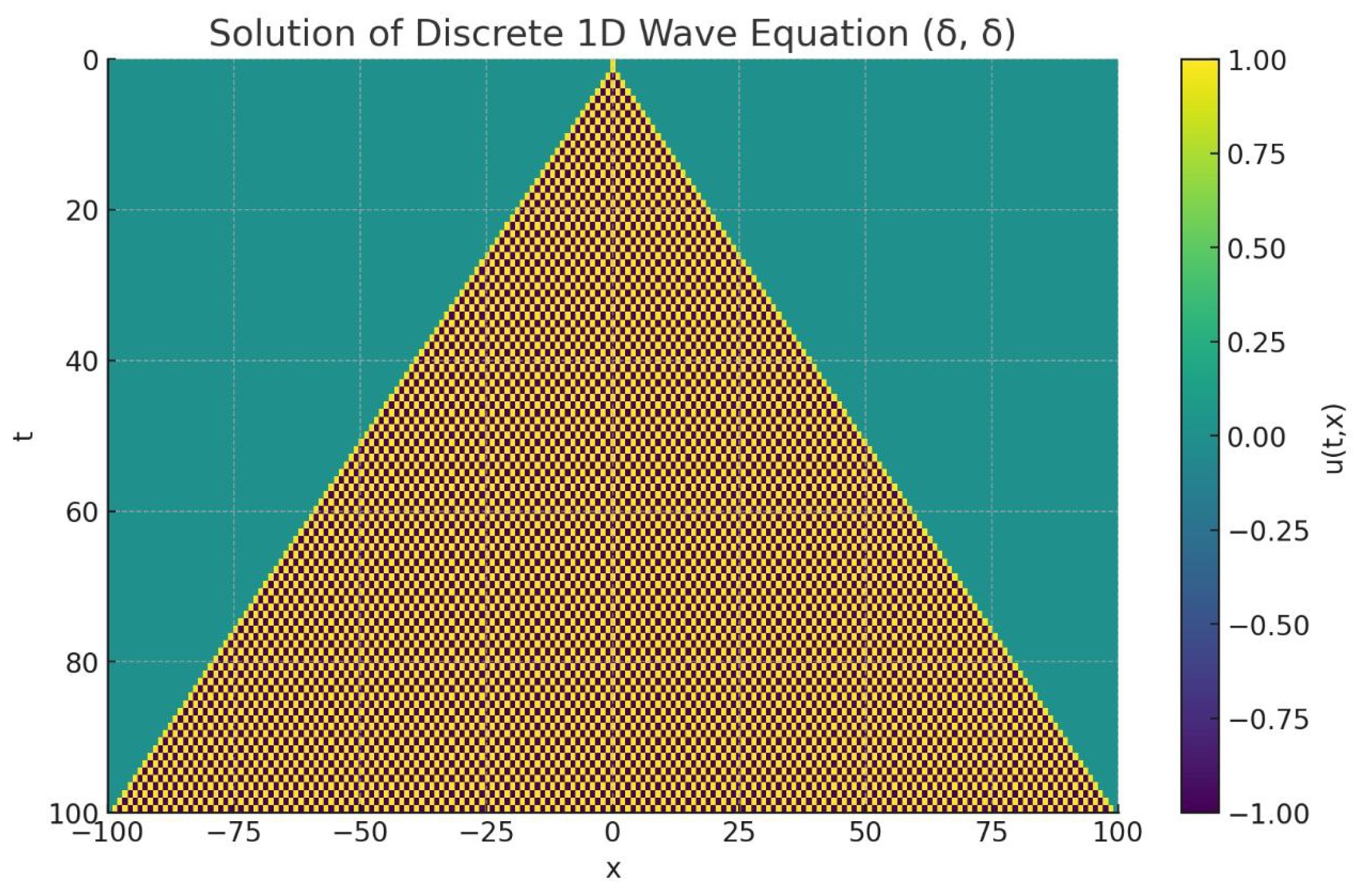
2.4. Discrete 1D Wave Equation

The Discrete 1D Wave Equation models undamped wave propagation on a one-dimensional lattice:

$$E_{t}u=E_x^{-1}u+E_{x}u-E_t^{-1}u$$

with initial conditions:

$$u(0,x)=\delta \left(x\right),u(1,x)=\delta \left(x\right)$$

and no boundary condition (i.e., defined on the full lattice $\mathbb{Z}$).

Exact Solution:

$$u(t,x)={(-1)}^{\left|x\right|+t}·\mathrm{com}(x,t)$$

where $\mathrm{com}(x,t)$ is a compact support indicator function defined by:

$$\mathrm{com}(x,a):=\left\{\begin{array}{cc}1,\hfill & \mathrm{if}\left|x\right|\le a\hfill \\ 0,\hfill & \mathrm{otherwise}\hfill \end{array}\right.$$

This can be generalized to be centered at an arbitrary point $x_0$:

$$\mathrm{com}(x-x_0,a):=\left\{\begin{array}{cc}1,\hfill & \mathrm{if}|x-x_0|\le a\hfill \\ 0,\hfill & \mathrm{otherwise}\hfill \end{array}\right.$$

The alternating sign ${(-1)}^{\left|x\right|+t}$ introduces a checkerboard-like structure in the wave propagation, while the compact support ensures finite spread with speed 1.

Figure 1. Spatiotemporal plot of the 1D Wave Equation

Figure 1. Spatiotemporal plot of the 1D Wave Equation

3. A General Framework for Linear Partial Difference Equations

In this section, we will define Difference Operator, Shift Operator, Discrete Hilbert Space, Adjoints, and Green’s Function, these concepts are inspired by Ordinary Difference Equations [1] and Partial Differential Equations [2].

3.1. The Difference Operator

Definition 4.1 (First-Order Difference Operator). Let $x\left(t\right)$ be a function defined on discrete time steps $t\in \mathbb{Z}$. The first-order (forward) difference operator is defined by:

$$\Delta x\left(t\right)=x(t+1)-x\left(t\right)$$

Definition 4.2 (Second-Order Difference Operator). The second-order difference is defined as the difference of the first-order differences:

$${\Delta }^{2}x\left(t\right)=\Delta x(t+1)-\Delta x\left(t\right)=x(t+2)-2x(t+1)+x\left(t\right)$$

This operator serves as the discrete analogue of the second derivative in classical calculus.

Definition 4.3 (Partial Difference Operators). Let $u(t,x)$ be a function defined on a discrete spacetime grid, where $(t,x)\in {\mathbb{Z}}^2$. The partial forward difference in time is defined by:

$${\Delta }_{t}u(t,x)=u(t+1,x)-u(t,x)$$

Similarly, the partial forward difference in space is defined by:

$${\Delta }_{x}u(t,x)=u(t,x+1)-u(t,x)$$

These partial difference operators serve as the fundamental components for constructing partial difference equations (P$\Delta$Es), which describe the evolution of discrete fields across both time and space.

3.2. The Shift Operator

The shift operator describes the translation of a function over discrete space or time.

Definition 4.1 (Shift Operator). Let $u\left(t\right)$ be a function defined on discrete time steps $t\in \mathbb{Z}$. The shift operator E is defined as:

$$Eu=u(t+1)$$

Definition 4.2 (Partial Shift Operators). For a function $u(t,x,y)$ defined on a discrete spacetime lattice, we define partial shift operators in each coordinate direction:

• Temporal shift (in time):

  $$E_{t}u=u(t+1,x,y)$$
• Spatial shift in the x-direction:

  $$E_{x}u=u(t,x+1,y)$$

Definition 4.3 (Higher-Order Shift Operators). The k-th order shift in the x-direction is defined by:

$$E_x^{k}u(t,x,y)=u(t,x+k,y)$$

Relation to the Difference Operator. The forward difference operator can be expressed using the shift operator as:

$$\Delta x\left(t\right)=x(t+1)-x\left(t\right)=Ex\left(t\right)-x\left(t\right)$$

Therefore,

$$\Delta =E-I,{\Delta }^2={(E-I)}^2$$

This formalism shows that the difference operator is derived from the shift operator as a deviation from the identity.

3.3. Representations of Difference Equations

Difference equations can be expressed in terms of difference operators or equivalently in terms of shift operators. The shift form emphasizes recurrence, while the difference form emphasizes change.

1. Representation Using Difference Operators

Example 1: A nonlinear first-order difference equation:

$$\Delta x\left(t\right)=rx\left(t\right)\left(1-x\left(t\right)\right)+x\left(t\right)$$

Example 2: A discrete diffusion equation in three spatial dimensions:

$${\Delta }_{t}u(t,x,y,z)={\Delta }_x^{2}u(t,x,y,z)+{\Delta }_y^{2}u(t,x,y,z)+{\Delta }_z^{2}u(t,x,y,z)$$

where $u=u(t,x,y,z)$ is the discrete field.

2. Representation Using Shift Operators

Example 1: The same nonlinear equation in shift form:

$$x(t+1)=rx\left(t\right)\left(1-x\left(t\right)\right)\Rightarrow Ex\left(t\right)=rx\left(t\right)\left(1-x\left(t\right)\right)$$

Example 2: The same spatial diffusion process in shift form:

$$u(t+1,x)=u(t,x-1)+u(t,x+1)\Rightarrow E_{t}u(t,x)=E_x^{-1}u(t,x)+E_{x}u(t,x)$$

These shift-form expressions are also called recurrence relations, since they express the value at a future step as a function of previous values using shift operators.

Equivalence Theorem

Theorem 1

(Equivalence of Difference Equations and Recurrence Relations). Any difference equation can be written as a recurrence relation using shift operators, and conversely, any recurrence relation can be written as a difference equation.

Proof. 

Let $u=u(t,x,y,z)$ be a discrete function defined on the lattice ${\mathbb{Z}}^4$.

A general difference equation may involve finite-order partial differences in time and space:

$$F\left(u,{\Delta }_{t}u,{\Delta }_t^{2}u,\dots ,{\Delta }_t^{k}u,{\Delta }_{x}u,{\Delta }_x^{2}u,\dots ,{\Delta }_x^{k}u,{\Delta }_{y}u,\dots ,{\Delta }_y^{k}u,{\Delta }_{z}u,\dots ,{\Delta }_z^{k}u\right)=0$$

Using the identity ${\Delta }_i=E_i-I$ (for $i\in \{t,x,y,z\}$), we can rewrite each difference term as:

$${\Delta }_i^{k}u={(E_i-I)}^{k}u$$

Thus the equation becomes:

$$F\left(u,(E_t-I)u,{(E_t-I)}^{2}u,\dots ,{(E_x-I)}^{k}u,\dots \right)=0$$

which is equivalent to a recurrence relation of the form:

$$G\left(u,E_{t}u,E_t^{2}u,\dots ,E_{x}u,E_x^{2}u,\dots ,E_y^{k}u,E_z^{k}u\right)=0$$

Conversely, given a recurrence relation:

$$P\left(u,E_{t}u,E_t^{2}u,\dots ,E_{x}u,\dots ,E_x^{k}u,E_{y}u,\dots ,E_y^{k}u,E_z^{k}u\right)=0$$

we substitute $E_i={\Delta }_i+I$, yielding:

$$P\left(u,({\Delta }_t+I)u,{({\Delta }_t+I)}^{2}u,\dots \right)=0$$

This can be rearranged as a difference equation:

$$Q\left(u,{\Delta }_{t}u,{\Delta }_t^{2}u,\dots ,{\Delta }_x^{k}u,{\Delta }_y^{k}u,{\Delta }_z^{k}u\right)=0$$

Hence, both representations are equivalent. □

3.4. Principle of Linear Superposition

Theorem 2

(Difference Operator is a Linear Operator). The difference operator Δ and its higher-order powers ${\Delta }^k$ are linear operators on discrete functions.

Proof. 

Let $u\left(t\right)$ and $v\left(t\right)$ be discrete functions, and let $a,b\in \mathbb{R}$ (or $\mathbb{C}$). The forward difference operator is defined by:

$$\Delta f\left(t\right)=f(t+1)-f\left(t\right)$$

We compute:

$$\Delta [au+bv]\left(t\right)=(au+bv)(t+1)-(au+bv)\left(t\right)=au(t+1)+bv(t+1)-au\left(t\right)-bv\left(t\right)$$

$$=a\left[u\right(t+1)-u(t\left)\right]+b\left[v\right(t+1)-v(t\left)\right]=a\Delta u\left(t\right)+b\Delta v\left(t\right)$$

Thus, $\Delta$ is linear. Since ${\Delta }^k$ is defined recursively as ${\Delta }^{k}f=\Delta \left({\Delta }^{k-1}f\right)$, and each $\Delta$ is linear, it follows by induction that ${\Delta }^k$ is also linear. □

Theorem 3

(Shift Operator is a Linear Operator). The shift operator E and its powers $E^k$ are linear operators on discrete functions.

Proof. 

Let $u\left(t\right)$ and $v\left(t\right)$ be discrete functions, and let $a,b\in \mathbb{R}$ (or $\mathbb{C}$). The shift operator is defined by:

$$Ef\left(t\right)=f(t+1)$$

Then:

$$E[au+bv]\left(t\right)=(au+bv)(t+1)=au(t+1)+bv(t+1)=aEu\left(t\right)+bEv\left(t\right)$$

Therefore, E is linear. The powers $E^k$ are defined as repeated application of E, so:

$$E^k[au+bv]\left(t\right)=a{E}^{k}u\left(t\right)+b{E}^{k}v\left(t\right)$$

Thus, $E^k$ is also linear. □

Solution Space

Theorem 4

(Solution Space is a Vector Space). The set of solutions to a linear partial difference equation forms a vector space.

Proof. 

Let the equation be given by:

$$L\left(u\right)=\sum _{(n,i,j,k)\in S}\left(a_n{E}_t^{n}u+a_i{E}_x^{i}u+a_j{E}_y^{j}u+a_k{E}_z^{k}u\right)=0$$

where S is a finite index set, and $a_n,a_i,a_j,a_k\in \mathbb{R}$ (or $\mathbb{C}$). The operator L is linear by construction.

Let v and w be solutions of the equation:

$$L\left(v\right)=0,L\left(w\right)=0$$

Let $a,b\in \mathbb{R}$ (or $\mathbb{C}$). Then by the linearity of L:

$$L(av+bw)=L\left(av\right)+L\left(bw\right)=aL\left(v\right)+bL\left(w\right)=a·0+b·0=0$$

Therefore, $av+bw$ is also a solution. The solution set is closed under addition and scalar multiplication, and thus forms a vector space. □

3.5. Discrete Hilbert Space

Definition 7

(Discrete Hilbert Space). Let ${\mathsf{\ell }}^2\left({\mathbb{Z}}^n\right)$ denote the set of complex-valued functions $u:{\mathbb{Z}}^n\to \mathbb{C}$ such that

$$\sum _{\mathbf{x}\in {\mathbb{Z}}^n}{\left|u\left(\mathbf{x}\right)\right|}^2<\infty .$$

This space is equipped with the inner product

$$\langle u,v\rangle =\sum _{\mathbf{x}\in {\mathbb{Z}}^n}\overline{u\left(\mathbf{x}\right)}v\left(\mathbf{x}\right),$$

which makes ${\mathsf{\ell }}^2\left({\mathbb{Z}}^n\right)$ a Hilbert space.

3.6. Adjoints

Definition 8

(Adjoint Operator). Let T be a bounded linear operator on a Hilbert space $\mathcal{H}={\mathsf{\ell }}^2\left({\mathbb{Z}}^n\right)$. The adjoint of T, denoted $T^{*}$, is defined by the relation

$$\langle Tu,v\rangle =\langle u,T^{*}v\rangle$$

for all $u,v\in \mathcal{H}$.

Proposition 1.

The shift operator E satisfies $E^{*}=E^{-1}$.

Proof. 

Let $Eu\left(x\right)=u(x+1)$. Then

$$\langle Eu,v\rangle =\sum _x\overline{u(x+1)}v\left(x\right)=\sum _x\overline{u\left(x\right)}v(x-1)=\langle u,E^{-1}v\rangle .$$

Hence $E^{*}=E^{-1}$. □

Proposition 2.

The forward difference operator $\Delta :=E-I$ has adjoint ${\Delta }^{*}=-\nabla$, where $\nabla :=I-E^{-1}$ is the backward difference.

3.7. The Kronecker Delta Function

Definition 9

(Univariate Kronecker Delta). The Kronecker delta function is defined as

$$\delta (x-a)=\left\{\begin{array}{cc}1,\hfill & \mathrm{if}x=a\hfill \\ 0,\hfill & \mathrm{otherwise}\hfill \end{array}\right.$$

for any $x,a\in \mathbb{Z}$.

Definition 10

(Multivariate Kronecker Delta). The multivariate Kronecker delta function is defined as the product of independent univariate deltas:

$$\delta (x-a,y-b)=\delta (x-a)\delta (y-b)$$

$$\delta (x-a,y-b,z-c)=\delta (x-a)\delta (y-b)\delta (z-c)$$

$$\delta (t-k,x-a,y-b,z-c)=\delta (t-k)\delta (x-a)\delta (y-b)\delta (z-c)$$

Proposition 3

(Delta Representation of Discrete Functions). Any function $f:\mathbb{Z}\to \mathbb{R}$ can be written as a sum over Kronecker deltas:

$$f\left(x\right)=\sum _{s\in \mathbb{Z}}f\left(s\right)\delta (x-s)$$

Similarly, any multivariate function $f:{\mathbb{Z}}^4\to \mathbb{R}$ can be expanded as

$$f(t,x,y,z)=\sum _{(k,a,b,c)\in {\mathbb{Z}}^4}f(k,a,b,c)\delta (t-k,x-a,y-b,z-c)$$

3.8. The Green’s Function

Definition. Consider a linear partial difference equation of the form:

$$E_{t}u=a{E}_x^{-1}u+bu+c{E}_{x}u$$

with the initial condition:

$$u(0,x)=\delta \left(x\right)$$

where $\delta \left(x\right)$ is the Kronecker delta function. If a function $G(t,x)$ satisfies this equation under the given initial condition (with or without boundary conditions), then $G(t,x)$ is called the Green’s function of the system.

Theorem 5.

If $G(t,x)$ is the Green’s function for a linear partial difference equation with initial condition $u(0,x)=\delta \left(x\right)$ and no boundary conditions, then for any arbitrary initial condition $u(0,x)=f\left(x\right)$, the general solution is given by:

$$u(t,x)=\sum _{s\in \mathbb{Z}}f\left(s\right)G(t,x-s)$$

Proof.

1.

If the initial impulse $\delta \left(x\right)$ is shifted to $\delta (x-s)$, the resulting solution is correspondingly shifted to $G(t,x-s)$ due to translation invariance.

2.

By the principle of linear superposition, the linear combination of solutions corresponding to each shifted impulse yields the solution for arbitrary initial data:

$$f\left(x\right)=\sum _{s\in \mathbb{Z}}f\left(s\right)\delta (x-s)\Rightarrow u(t,x)=\sum _{s\in \mathbb{Z}}f\left(s\right)G(t,x-s)$$

□

3.9. Boundary Value Problems

In this paper, we will only focus on Dirichlet Boundary Condition.

Dirichlet Boundary Condition

Definition. The Dirichlet boundary condition specifies the value of the function on the boundary of the spatial domain. In discrete systems, this corresponds to assigning fixed values at the boundary points.

1D Example. Consider a 1D discrete domain $x\in \{0,1,\dots ,N\}$. A Dirichlet boundary condition takes the form:

$$u(t,0)=a,u(t,N)=b,$$

where a and b are given constants.

2D Example. Let $(x,y)\in \{0,1,\dots ,N\}\times \{0,1,\dots ,M\}$. A Dirichlet boundary condition specifies:

$$u(t,0,y)=f_1\left(y\right),u(t,N,y)=f_2\left(y\right),u(t,x,0)=g_1\left(x\right),u(t,x,M)=g_2\left(x\right).$$

3D Example. Let $(x,y,z)\in \{0,\dots ,N\}\times \{0,\dots ,M\}\times \{0,\dots ,L\}$. Then the Dirichlet condition prescribes:

$$\begin{array}{cc}& u(t,0,y,z)=f_1(y,z),u(t,N,y,z)=f_2(y,z),\hfill \\ & u(t,x,0,z)=g_1(x,z),u(t,x,M,z)=g_2(x,z),\hfill \\ & u(t,x,y,0)=h_1(x,y),u(t,x,y,L)=h_2(x,y).\hfill \end{array}$$

The Impact of Boundary Conditions

We observe that the choice of boundary condition significantly affects the evolution of the system.

For example, consider Rule 90, a one-dimensional cellular automaton with a single-point initial condition. When no boundary condition is imposed (e.g., an infinite domain), the evolution produces a perfectly self-similar fractal pattern, known as the Sierpiński triangle.

However, when a fixed boundary condition is imposed (e.g., $u(t,0)=0$, $u(t,N)=0$), the system’s symmetry is broken, and the resulting pattern becomes irregular or even chaotic.

This highlights how boundary conditions can destroy or preserve global structure in discrete dynamical systems.

4. 1D Cellular Automata

4.1. Introduction

The study of one-dimensional cellular automata (1D CA) was significantly advanced by Stephen Wolfram [3], who systematically explored the behavior of all 256 elementary rules. These models, despite their simplicity, can generate a wide range of complex spatiotemporal patterns, including periodic structures, nested fractals, localized structures, and even chaotic behavior.

All 1D cellular automata can be expressed as autonomous partial difference equations, meaning that the update rule does not include any external forcing term. Moreover, most of these equations are inherently nonlinear, due to the logical (Boolean) nature of the local interactions.

In this section, we formulate several 1D cellular automata as partial difference equations. Some of these formulations are based on known Boolean algebra transformations, converting logical rules into Boolean polynomials, and then into partial difference equations. Others are derived heuristically by observing the pattern of evolution.

This reformulation has several important advantages:

• It provides a unified mathematical framework to study discrete systems.
• It allows the application of analytical tools such as operator theory, stability analysis, and even Green’s functions.
• It enables the exploration of different types of initial and boundary conditions in a more formalized way.
• It makes it possible to introduce non-autonomous terms and study how external forcing influences the evolution.

This approach transforms cellular automata from mere computational toys into objects of rigorous mathematical investigation within the broader context of discrete dynamical systems.

4.2. The Rule 90

The Rule 90 cellular automaton can be written as a nonlinear partial difference equation of the form:

$$E_{t}u={\mathrm{mod}}_2\left(E_x^{-1}u+E_{x}u\right)$$

where ${\mathrm{mod}}_2\left(x\right)$ is defined as:

$${\mathrm{mod}}_2\left(x\right):=\left\{\begin{array}{cc}1,\hfill & \mathrm{if}x\mathrm{is}\mathrm{odd}\hfill \\ 0,\hfill & \mathrm{if}x\mathrm{is}\mathrm{even}\hfill \end{array}\right.$$

This function is clearly nonlinear, making the equation itself nonlinear.

We refer to this equation as the Sierpiński Equation, due to its deep connection with the Sierpiński triangle.

Define a discrete delta function as:

$$\delta (x-a):=\left\{\begin{array}{cc}1,\hfill & \mathrm{if}x=a\hfill \\ 0,\hfill & \mathrm{otherwise}\hfill \end{array}\right.$$

Given the initial condition $u(0,x)=\delta \left(x\right)$ and no boundary condition, the exact solution to the equation is:

$$u(t,x)=C(2t,x+t)mod2$$

where $C(x,y)$ is the binomial coefficient, defined as:

$$C(x,y):=\left\{\begin{array}{cc}{\displaystyle \frac{x!}{(x-y)!y!}},\hfill & \mathrm{if}0\le y\le x\hfill \\ 0,\hfill & \mathrm{otherwise}\hfill \end{array}\right.$$

For a general initial condition $u(0,x)=f\left(x\right)$, the solution becomes:

$$u(t,x)=\sum _{s\in \mathbb{Z}}f\left(s\right)·C(2t,x+t-s)mod2$$

This system exhibits chaotic behavior in a discrete binary field. Remarkably, despite its chaotic dynamics, we have found a closed-form analytical solution. This provides a foundation to define and analyze concepts like chaotic functions and quasichaotic functions within the framework of discrete functional analysis.

Example 1

This is the spatiotemporal plot of Rule 90 with the initial condition $u(0,x)=\delta \left(x\right)$ and no boundary conditions.

Figure 2. Spatiotemporal plot of Rule 90 with $u(0,x)=\delta \left(x\right)$ and no boundary conditions.

Figure 2. Spatiotemporal plot of Rule 90 with $u(0,x)=\delta \left(x\right)$ and no boundary conditions.

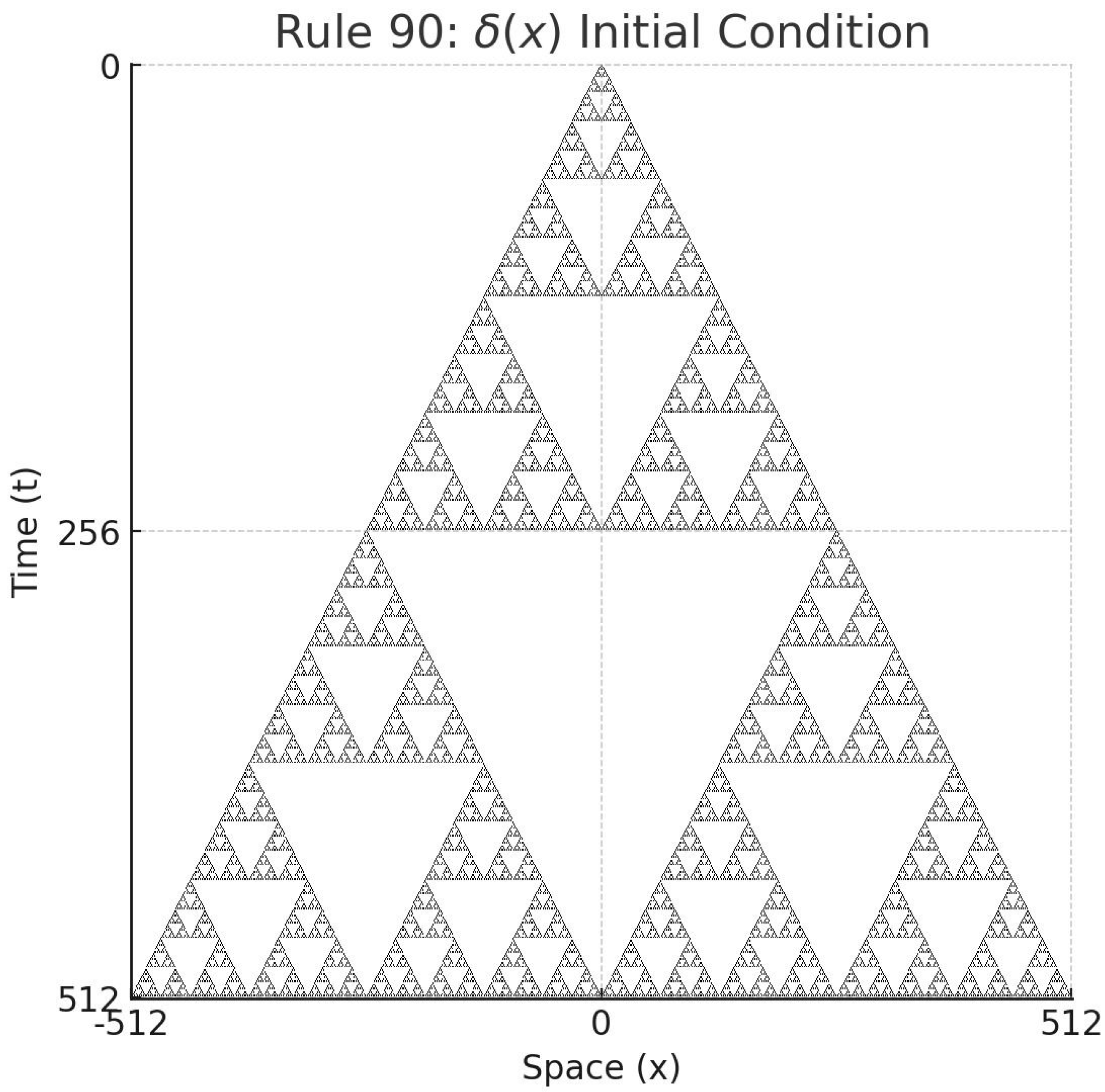
It clearly forms a Sierpiński triangle. Note that each cell’s state depends only on its left and right neighbors. Thus, this fractal is not globally planned, but emerges from local interactions.

Example 2

This is the spatiotemporal plot of Rule 90 with the initial condition $u(0,x)=\delta \left(x\right)$ and boundary conditions $u(t,-100)=u(t,100)=0$.

Figure 3. Spatiotemporal plot of Rule 90 with $u(0,x)=\delta \left(x\right)$ and boundary conditions $u(t,-100)=u(t,100)=0$.

Figure 3. Spatiotemporal plot of Rule 90 with $u(0,x)=\delta \left(x\right)$ and boundary conditions $u(t,-100)=u(t,100)=0$.

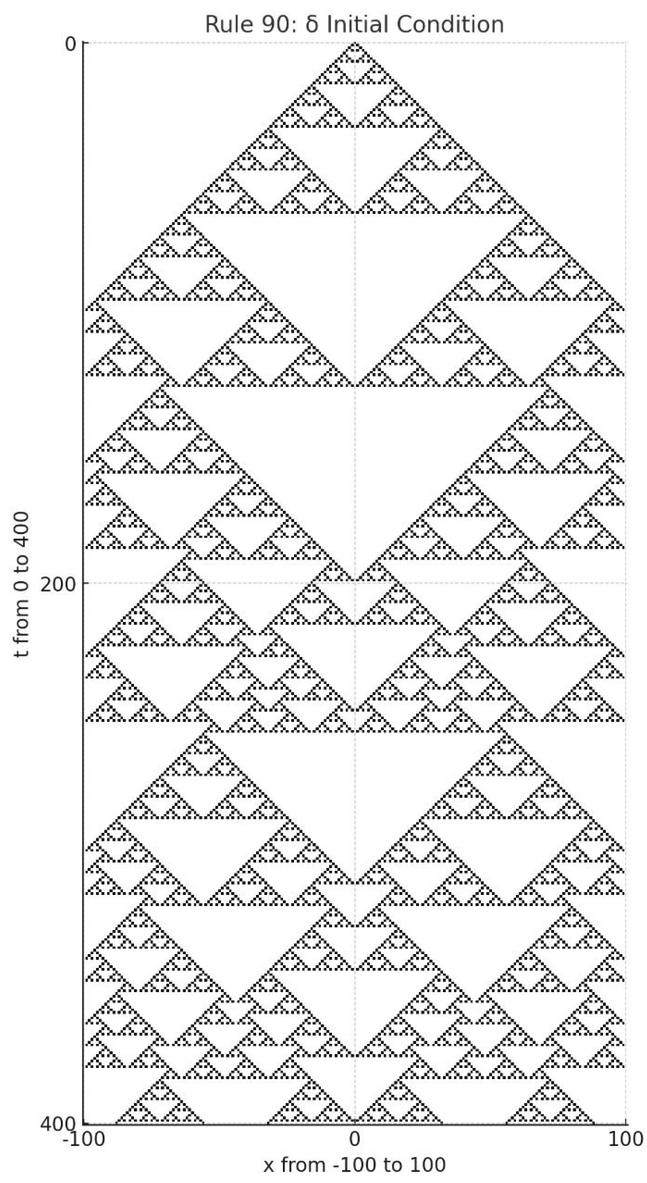
Initially, we observe a perfect Sierpiński triangle. However, once the pattern reaches the boundary, it breaks down into spatiotemporal chaos and becomes unpredictable.

Example 3

This is the spatiotemporal plot of Rule 90 with random initial condition and boundary conditions $u(t,-200)=u(t,200)=0$.

Figure 4. Spatiotemporal plot of Rule 90 with random initial condition and boundary conditions.

Figure 4. Spatiotemporal plot of Rule 90 with random initial condition and boundary conditions.

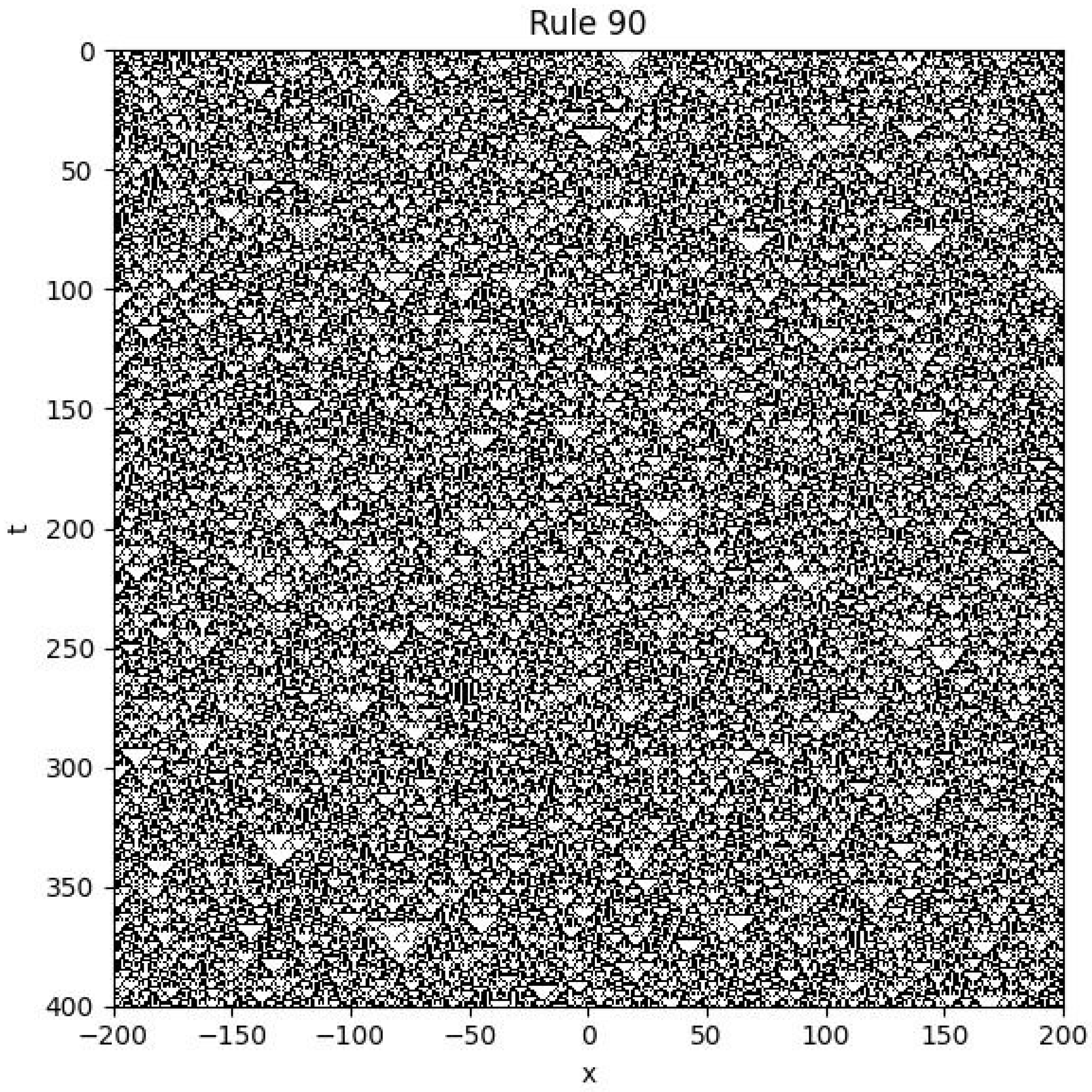
As shown, the system exhibits spatiotemporal chaos.

4.3. Rule 30

The evolution equation for Rule 30, derived using Boolean algebra, is given by:

$$E_{t}u={mod}_2\left(E_x^{-1}u+E_{x}u+u+u·E_{x}u\right),$$

where $E_t$ is the time shift operator, $E_x$ is the spatial right shift operator, and all operations are over the binary field ${\mathbb{F}}_2$ (i.e., modulo 2).

Example

We consider the following simulation setup:

• Initial condition: $u(0,x)$ is chosen randomly with values in $\{0,1\}$.
• Boundary condition: $u(t,-200)=u(t,200)=0$ for all t.

The figure below shows the spatiotemporal evolution of the system under Rule 30:

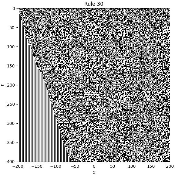
It is evident that the system exhibits spatiotemporal chaos, characterized by aperiodic and unpredictable patterns across both space and time.

4.4. The Rule 153

We define the evolution equation as follows:

$$E_{t}u={mod}_2\left(⌊{\displaystyle \frac{1-E_x^{-1}u}{1+E_{x}u}}+E_{x}u·E_x^{-1}u+\left|3E_x^{-1}u-4E_{x}u\right|+u⌋\right)$$

Example

• Initial condition: $u(0,x)$ is assigned a random binary value (0 or 1) at each spatial point.
• Boundary condition: $u(t,-200)=u(t,200)=0$ for all t.
• Color scheme: 0 is shown as white, and 1 is shown as black.

The following image illustrates the space-time evolution from $t=0$ to $t=400$, and $x\in [-200,200]$, with a random initial condition:

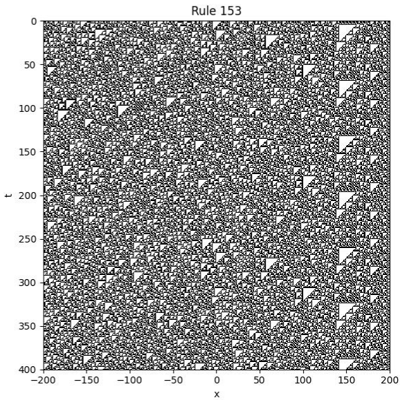
This system exhibits spatiotemporal chaos.

4.5. Rule 45

The Boolean update rule for Rule 45 can be written as the following equation:

$$E_{t}u={\mathrm{mod}}_2\left(1+u+E_x^{-1}u+u·E_{x}u\right)$$

Example

Initial condition: $u(0,x)$ is random.

Boundary conditions: $u(t,-200)=u(t,200)=0$.

Figure 5. Spatiotemporal plot of Rule 45 with random initial condition and fixed boundary conditions.

Figure 5. Spatiotemporal plot of Rule 45 with random initial condition and fixed boundary conditions.

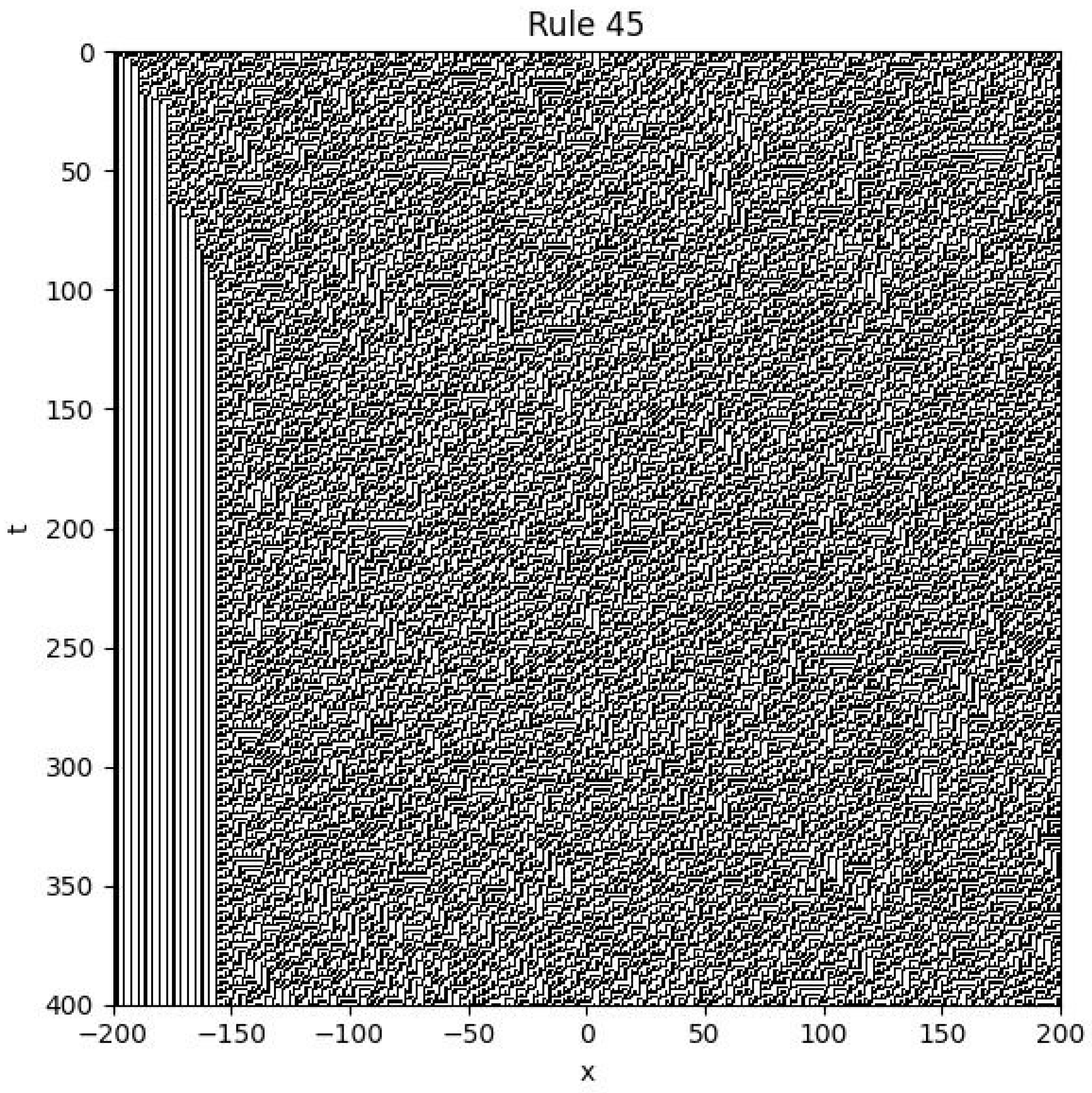
As shown in the figure, this system also exhibits spatiotemporal chaos. The resulting pattern features strange, curled, filament-like structures.

4.6. Rule 105

The Boolean update rule for Rule 105 can be written using logical operations as follows:

$$E_{t}u={\mathrm{mod}}_2\left(E_x^{-1}u·u·\delta \left(E_{x}u\right)+E_x^{-1}u·\delta \left(u\right)·E_{x}u+\delta \left(E_x^{-1}u\right)·u·E_{x}u+\delta \left(E_x^{-1}u\right)·\delta \left(u\right)·\delta \left(E_{x}u\right)\right)$$

Here, $\delta \left(x\right):=1+x\left(\mathrm{mod}2\right)$ denotes the Boolean NOT operation.

Example

Initial condition: $u(0,x)$ is random.

Boundary conditions: $u(t,-200)=u(t,200)=0$.

Figure 6. Spatiotemporal plot of Rule 105 with random initial condition and fixed boundaries.

Figure 6. Spatiotemporal plot of Rule 105 with random initial condition and fixed boundaries.

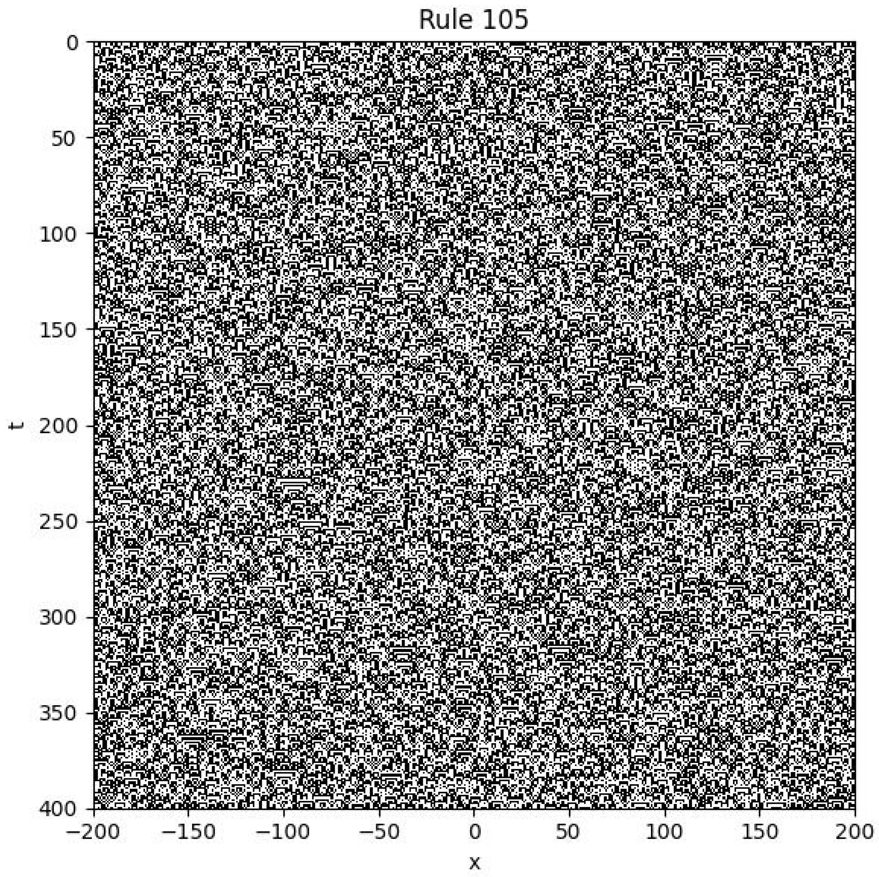
As shown in the figure, this system also exhibits spatiotemporal chaos. The resulting pattern consists of intricate structures resembling scales or rippling textures.

4.7. Rule 169

The Boolean update rule for Rule 169 can be expressed as:

$$E_{t}u={\mathrm{mod}}_2\left(E_x^{-1}u·u+E_x^{-1}u+u+E_{x}u+1\right)$$

Example

Initial condition: $u(0,x)$ is random.

Boundary conditions: $u(t,-200)=u(t,200)=0$.

Figure 7. Spatiotemporal plot of Rule 169 with random initial condition and fixed boundaries.

Figure 7. Spatiotemporal plot of Rule 169 with random initial condition and fixed boundaries.

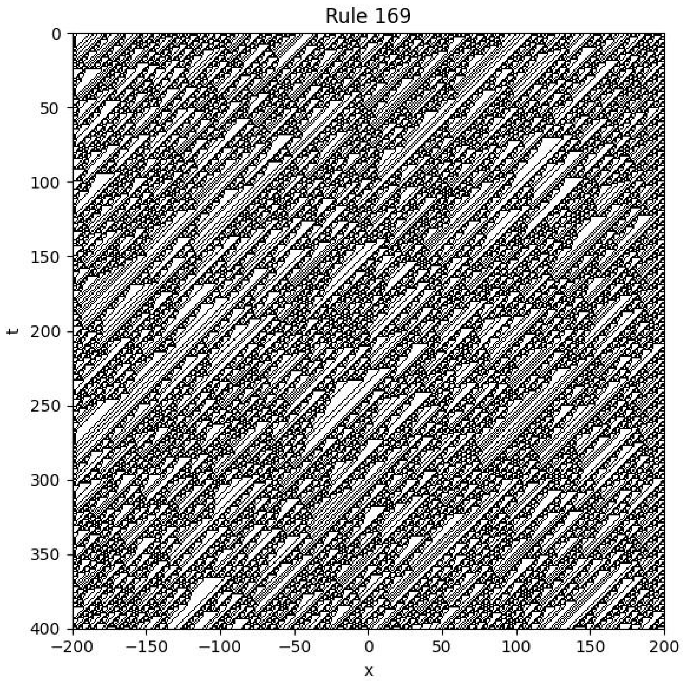
As shown in the figure, the system exhibits spatiotemporal chaos. The resulting patterns resemble diagonal stalactites, indicating complex local interactions and emergent behaviour.

4.8. Rule 210

The Boolean update rule for Rule 210 is given by:

$$E_{t}u={\mathrm{mod}}_2\left(E_x^{-1}u·u·E_{x}u+E_x^{-1}u·u·\delta \left(E_{x}u\right)+E_x^{-1}u·\delta \left(u\right)·\delta \left(E_{x}u\right)+\delta \left(E_x^{-1}u\right)·\delta \left(u\right)·E_{x}u\right)$$

Example

Initial condition: $u(0,x)$ is random.

Boundary conditions: $u(t,-200)=u(t,200)=0$.

Figure 8. Spatiotemporal plot of Rule 210 with random initial condition and fixed boundaries.

Figure 8. Spatiotemporal plot of Rule 210 with random initial condition and fixed boundaries.

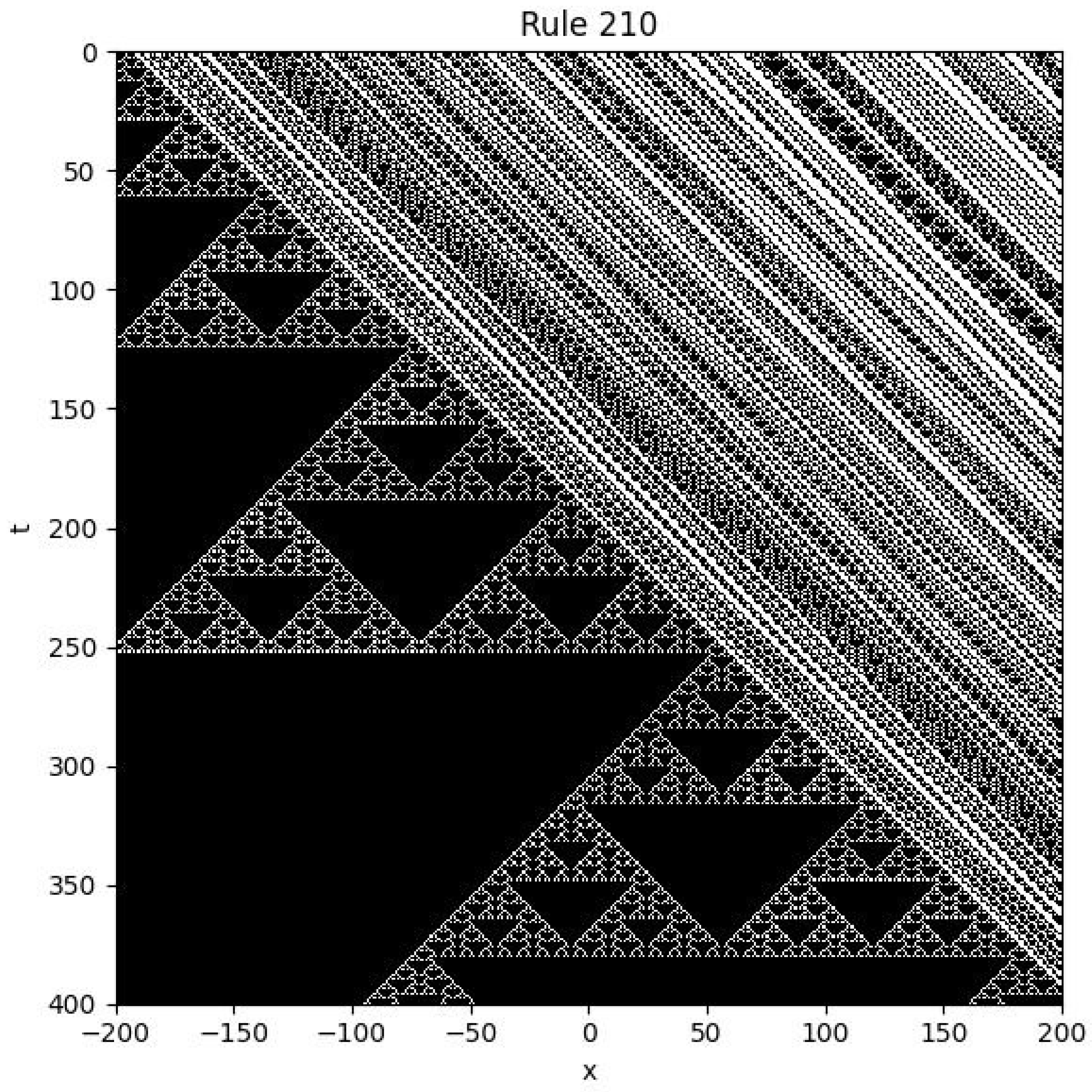
As shown in the figure, the system exhibits a highly unusual structure: one region resembles a Sierpiński triangle, while the other shows diagonally arranged motifs. This dual pattern reflects complex local interactions and potentially bifurcating spatial dynamics.

4.9. Rule 137

We define the evolution equation as follows:

$$E_{t}u={mod}_2\left(\left|⌊\left(E_x^{-1}u-{\pi }^u\right)\left(\pi +u+E_x\right)⌋\right|+⌊\left|{\displaystyle \frac{1-u}{1+u}}\right|⌋+\left|3E_x^{-1}u-4u\right|\right)$$

each state value satisfies

$$u(t,x)\in \{0,1\}.$$

This rule is an example of a nonlinear partial difference equation, operating over a binary state space.

Interestingly, the system exhibits a mixture of order and apparent randomness. Some regions evolve into highly regular patterns, while others appear chaotic and unpredictable. This suggests that the system may operate near the edge of chaos, a regime known for its potential computational richness and complexity.

Although we do not currently possess a closed-form analytic solution to this equation, the intricate structure of its evolving patterns can still be studied using tools such as combinatorics, discrete functional analysis, and spatiotemporal statistics.

Example

Initial condition: $u(0,x)$ is random.

Boundary conditions: $u(t,-200)=u(t,200)=0$.

Figure 9. Spatiotemporal plot of Rule 137 with random initial condition and fixed boundaries.

Figure 9. Spatiotemporal plot of Rule 137 with random initial condition and fixed boundaries.

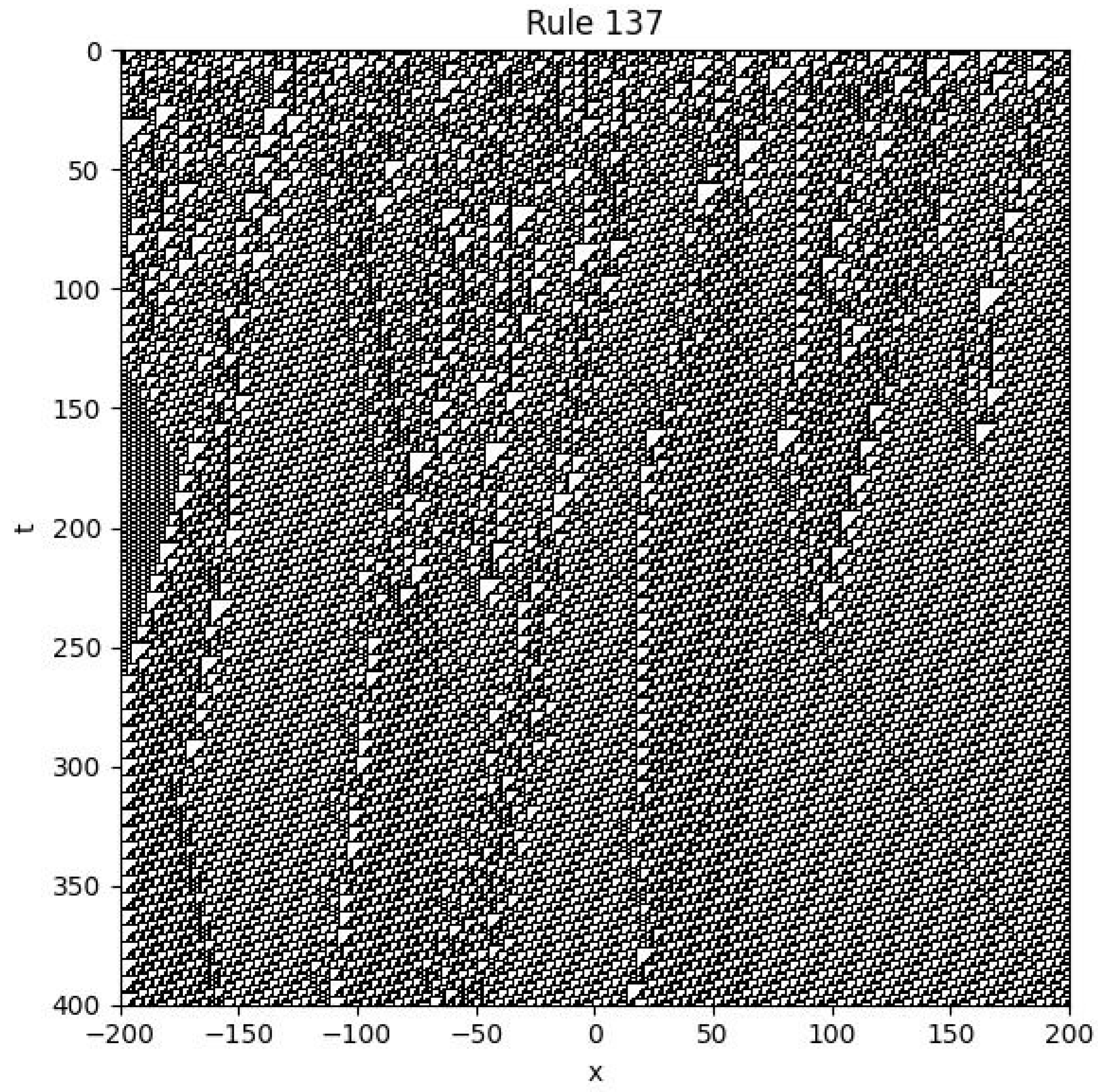
The pattern generated by Rule 137 closely resembles that of Rule 110. It exhibits complex behavior with both periodic islands and chaotic seas. There are large regions of crystalline structure, along with distinct triangular motifs, indicating rich dynamics and spatial self-organization.

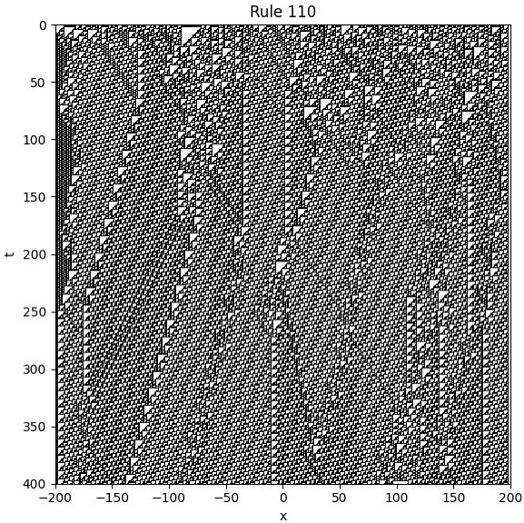
4.10. Rule 110

Using Boolean algebra, we derive the evolution equation for Rule 110 as follows:

$$E_{t}u={mod}_2\left(u+E_{x}u+u·E_{x}u+u·E_{x}u·E_x^{-1}u\right),$$

where $E_t$ denotes the time shift operator, $E_x$ is the spatial right-shift operator, and ${mod}_2$ denotes addition modulo 2.

Example

We consider the following setup:

• Initial condition: $u(0,x)$ is chosen randomly with values in $\{0,1\}$.
• Boundary condition: $u(t,-200)=u(t,200)=0$ for all t.

The figure below illustrates the space-time evolution of the system under Rule 110:

4.11. Remarks

For a more detailed study of one dimensional cellular automata in the form of partial difference equations, see [4].

5. Other 1D Nonlinear Partial Difference Equations

5.1. Introduction

Beyond classical two-state cellular automata such as Rule 90 or Rule 137, I have discovered that a wide variety of other one dimensional nonlinear partial difference equations (P$\Delta$Es) can be constructed. These equations may involve arithmetic operations, logical operations, or floor and absolute value functions. They do not necessarily follow the strict rule-based framework of cellular automata, yet they remain fully deterministic and discrete in both space and time.

Such equations often exhibit rich and unexpected dynamical behavior. Some generate spatially localized chaos, while others display periodic or quasiperiodic structures. This diversity suggests that one-dimensional nonlinear P$\Delta$Es form a broader and more general class of systems than traditionally studied automata.

In the following subsections, we will explore several such examples and discuss their qualitative features.

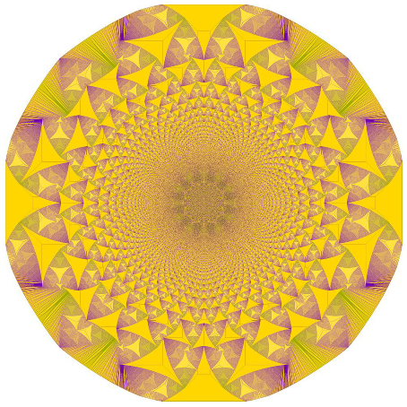
5.2. Sierpinski Fan Equation

Consider the following nonlinear partial difference equation:

$$E_{t}u=\left(E_x^{-1}u+u+E_{x}u\right)mod3$$

with initial condition:

$$u(0,x)=\delta \left(x\right),\mathrm{and}\mathrm{no}\mathrm{boundary}\mathrm{condition}.$$

Here, the delta function $\delta \left(x\right)$ is defined as:

$$\delta \left(x\right)=\left\{\begin{array}{cc}1,\hfill & x=0\hfill \\ 0,\hfill & x\ne 0\hfill \end{array}\right.$$

This system produces a fascinating fractal structure resembling a "fan" or "tree", hence we refer to it as the Sierpinski Fan Equation.

Although we currently do not have an analytic solution to this equation, the emergent pattern clearly exhibits self-similarity and modular periodicity, which are typical features of modular arithmetic-driven cellular automata. This suggests a rich underlying structure that deserves further investigation.

Figure 10. Spatiotemporal evolution of the Sierpinski Fan Equation

Figure 10. Spatiotemporal evolution of the Sierpinski Fan Equation

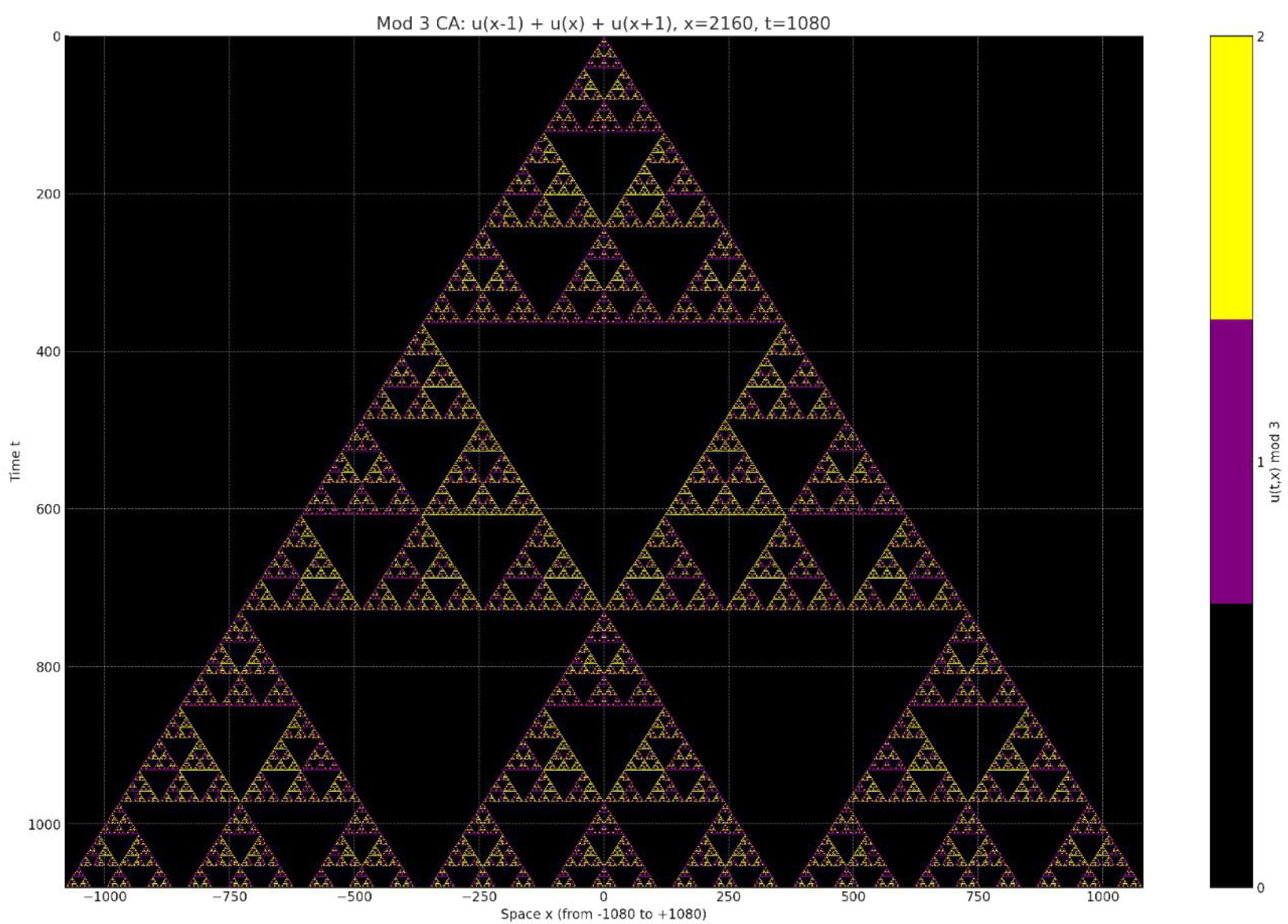
5.3. Mod 5 Sierpiński Equation

We define a new nonlinear partial difference equation as follows:

$$E_{t}u=\left(E_x^{-2}u+E_x^{-1}u+u+E_x^{1}u+E_x^{2}u\right)mod5$$

with the initial condition:

$$u(0,x)=\delta \left(x\right)$$

where:

• $\delta \left(x\right)$ is the discrete delta function defined by $\delta \left(x\right)=1$ if $x=0$, and 0 otherwise;
• $u(t,x)\in \{0,1,2,3,4\}$ for all $t,x$;
• The system is updated on a discrete 1D lattice with no boundary condition.

This equation can be seen as a generalization of the Rule 90 or Sierpiński triangle in modulo 2. The modulo 5 version creates a far richer fractal structure.

Figure 11. Spatiotemporal evolution of the Mod 5 Sierpiński Equation

Figure 11. Spatiotemporal evolution of the Mod 5 Sierpiński Equation

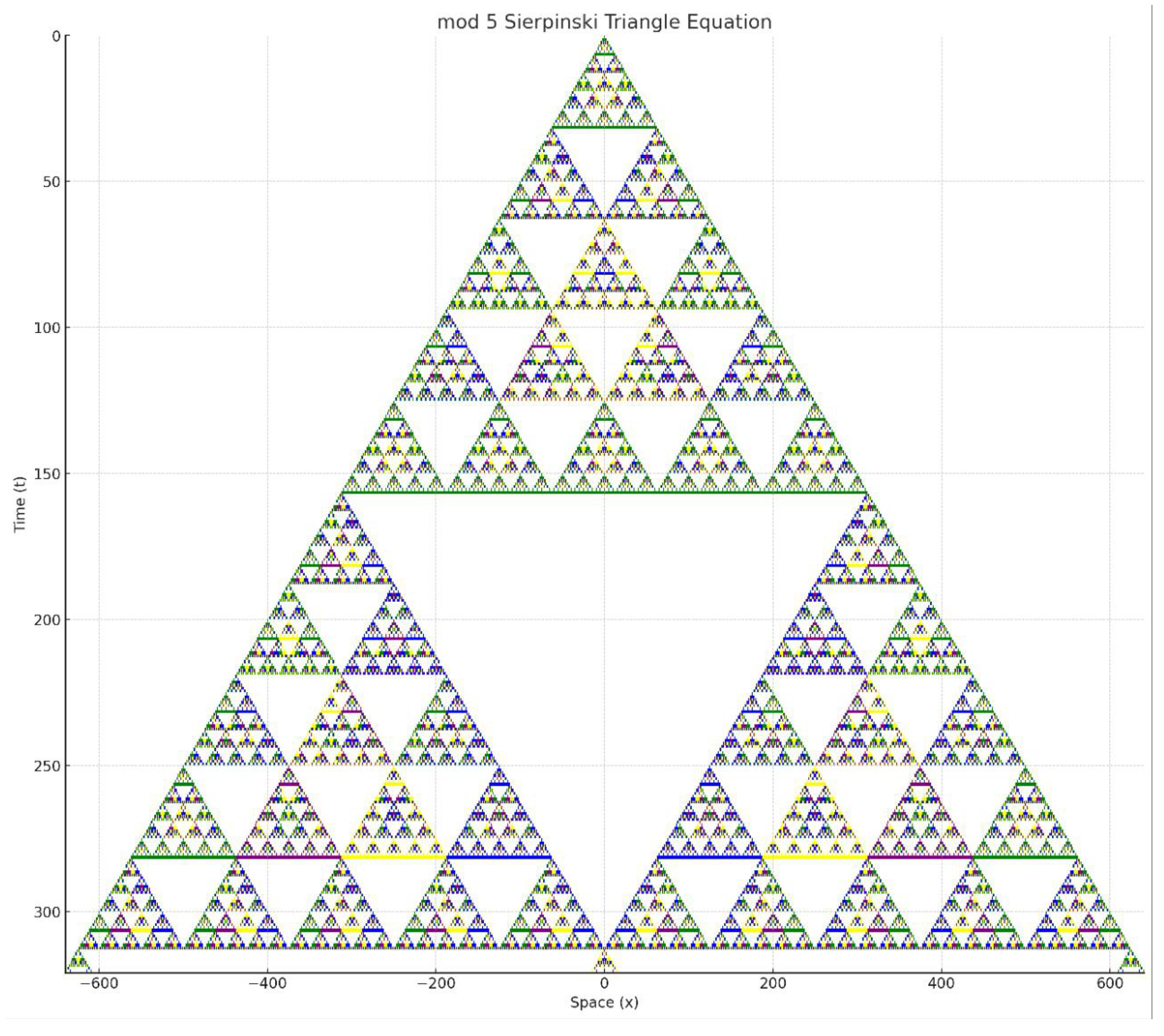
From the spatiotemporal plot, we observe that instead of the classic single upside-down triangle in each upright triangle (as in the binary Sierpiński triangle), this pattern exhibits ten upside-down triangles within each upright triangle. This suggests a more intricate self-similar structure with higher-order modular symmetry.

We call this the Mod 5 Sierpiński Equation.

5.4. Mod 4 Sierpinski Fractal Equation

We consider the following nonlinear partial difference equation:

$$E_{t}u=\left(E_x^{-1}u+u+E_{x}u+\delta \left(x\right)\right)mod4$$

with initial condition:

$$u(0,x)=\delta \left(x\right)$$

and no boundary condition.

Here, $\delta \left(x\right)$ is the discrete delta function defined by:

$$\delta \left(x\right)=\left\{\begin{array}{cc}1,\hfill & \mathrm{if}x=0\hfill \\ 0,\hfill & \mathrm{otherwise}\hfill \end{array}\right.$$

The values of $u(t,x)$ are restricted to $\{0,1,2,3\}$, and we visualize them using the following color scheme:

Value	Color
0	White
1	Green
2	Purple
3	Yellow

The spatiotemporal plot of this equation is shown below:

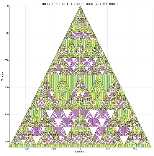
We observe that this system generates a strikingly complicated fractal structure, reminiscent of a Sierpinski triangle, but with richer periodic color layers. Despite its simplicity, the system exhibits highly nontrivial dynamics that may reflect deep combinatorial or algebraic patterns.

6. The Conway’s Game of Life

6.1. The Conway’s Equation

We can write Conway’s Game of Life as a nonlinear partial difference equation:

$$u(t+1,x,y)={\mathrm{mod}}_2\left(u(t,x,y)+\delta \left(F\right(S,u\left)\right)+G(S,u)\right)$$

where: - $u=u(t,x,y)\in \{0,1\}$ - $S={\sum }_{(i,j)\in M}u(t,x+i,y+j)$ is the sum over the Moore neighbourhood M - ${\mathrm{mod}}_2\left(x\right):=xmod2$ is defined as:

$${\mathrm{mod}}_2\left(x\right)=\left\{\begin{array}{cc}1,\hfill & \mathrm{if}x\mathrm{is}\mathrm{odd}\hfill \\ 0,\hfill & \mathrm{if}x\mathrm{is}\mathrm{even}\hfill \end{array}\right.$$

- $\delta \left(x\right)=1$ if $x=0$, and 0 otherwise - $F(S,u)$ and $G(S,u)$ are logic functions defined as:

$$F(S,1)=\left\{\begin{array}{cc}1,\hfill & \mathrm{if}S=2\mathrm{or}3\hfill \\ 0,\hfill & \mathrm{otherwise}\hfill \end{array}\right.G(S,0)=\left\{\begin{array}{cc}1,\hfill & \mathrm{if}S=3\hfill \\ 0,\hfill & \mathrm{otherwise}\hfill \end{array}\right.$$

In other words, the dynamics follow: - A live cell ($u=1$) survives if it has 2 or 3 neighbors. - A dead cell ($u=0$) becomes alive if it has exactly 3 neighbors.

6.2. Interpretation

This is an Autonomous Partial Difference Equation.

We observe that: - Gliders behave like solitons, stable moving structures. - Oscillators resemble standing waves, periodically repeating in place. - Each of these localized configurations can be seen as a local attractor unit. - Multiple local attractors can couple together, forming a large-scale network we call the Attractor Coupling Network (ACN).

This structure is: - A dynamic fractal network, in the sense that it exhibits recursive nesting: a network within a network, evolving over time. - Capable of universal computation: Conway’s Game of Life is known to be Turing complete.

This suggests a deep connection between simple discrete dynamics and the emergence of complex, structured, and computationally powerful behavior.

7. Abelian Sandpile Model

7.1. Abelian Sandpile Equation

The evolution of the Abelian Sandpile Model is given by the following equation:

$${\displaystyle E_{t}u=u-4\theta (u-4)+\sum _{(i,j)\in V}\theta \left(E_x^i{E}_y^{j}u-4\right)+G(t,x,y)}$$

where:

• $u(t,x,y)\in \{0,1,2,3\}$
• $\theta \left(x\right)$ is the Heaviside step function:

  $$\theta \left(x\right)=\left\{\begin{array}{cc}1,\hfill & \mathrm{if}x\ge 0\hfill \\ 0,\hfill & \mathrm{otherwise}\hfill \end{array}\right.$$
• V is the von Neumann neighbourhood:

  $$V=\left\{\right(1,0),(-1,0),(0,1),(0,-1\left)\right\}$$
• $G(t,x,y)$ is the external forcing term (i.e., the addition of sand grains)

7.2. Remarks

This is a Non-Autonomous Partial Difference Equation.

This is a classical model of Self-Organized Criticality (SOC). It exhibits:

• Emergent fractal patterns
• Scale-invariant avalanches
• Critical behavior without parameter fine-tuning

For a deeper understanding of self-organized criticality in sandpile models, see [5].

7.3. The Sandpile Fractal

If the forcing term is given by

$$G(t,x,y)=\delta \left(x\right)\delta \left(y\right),$$

with initial condition

$$u(0,x,y)=0,$$

and no boundary condition imposed, then the solution exhibits a fractal structure resembling the classical sandpile model. The resulting pattern looks as follows:

The picture is taken from Wikipedia.

7.4. Extended Sandpile Model

We present an extended version of the Abelian Sandpile Model in which each site topples only when it contains at least 8 grains of sand. The neighborhood used here is the Moore neighborhood, which includes the 8 surrounding cells (horizontal, vertical, and diagonal neighbors).

The evolution equation of the system is given by:

$$E_{t}u=u-8\theta (u-8)+\sum _{(i,j)\in \mathcal{M}}\theta (E_x^i{E}_y^{j}u-8)+G(t,x,y)$$

where:

• $u=u(t,x,y)$ represents the number of sand grains at position $(x,y)$ and time t,
• $\theta$ is the Heaviside step function,
• $\mathcal{M}$ denotes the Moore neighborhood:
  $M=\left\{\right(-1,-1),(-1,0),(-1,1),(0,-1),(0,1),(1,-1),(1,0),(1,1\left)\right\}$,
• $G(t,x,y)$ is an external sand input term.

Example

• Initial Condition:  $u(0,x,y)=0$
• Boundary Condition:  None (infinite or sufficiently large grid with no boundary constraints)
• Forcing Term: $G(t,x,y)=\delta \left(x\right)\delta \left(y\right)$ (unit sand grain dropped at the center)

The figure below shows the configuration $u(500000,x,y)$ after 500,000 iterations:

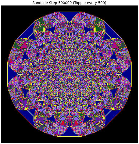
We observe that the resulting pattern resembles the classical sandpile model, but exhibits greater complexity due to the use of the Moore neighborhood and the 8-grain threshold. The colors are more diverse, and the structure appears more intricate and vibrant.

7.5. Explanation for the Self-Organized Criticality

Consider the comparison between Rule 90 and the Sandpile model. Rule 90 is defined by the update rule:

$$u(t+1,x)=\left(u(t,x-1)+u(t,x+1)\right)mod2$$

Both Rule 90 and the Sandpile model are based on local interactions and exhibit nonlinear dynamics. However, they display drastically different macroscopic behaviors: Rule 90 leads to global chaos, while the Sandpile model exhibits self-organized criticality.

In Rule 90, any small perturbation is exponentially amplified due to the absence of thresholds, every update directly sums the neighboring values modulo 2, regardless of the current state. As a result, the system exhibits global sensitivity to initial conditions, a hallmark of chaos.

In contrast, the Sandpile model incorporates a threshold-based collapse mechanism. Before any site reaches the threshold (typically 4 in 2D), the system behaves linearly: each grain of sand simply increases the local state by 1. Once the threshold is reached, a toppling event occurs, distributing sand to neighbors and potentially triggering further topplings. This collapse phase introduces nonlinearity and chaotic propagation, but only in localized regions that have reached the critical state.

Therefore, the Sandpile model alternates between two distinct regimes:

• Linear growth phase: Sites far below the threshold evolve smoothly and predictably.
• Chaotic collapse phase: Sites at the threshold trigger avalanches with unpredictable, nonlinear dynamics.

Because the initial configuration is typically random, some sites are near-zero (linear regime), while others are near the threshold (nonlinear regime). This coexistence of order and chaos in space and time allows the Sandpile model to maintain a dynamically balanced state without the need for fine-tuning of parameters.

This explains why the Sandpile model self-organizes into a critical state: the rules themselves inherently support a mixture of linear and chaotic zones, allowing the system to spontaneously hover at the edge of chaos. Unlike systems that require tuning to a critical point, the Sandpile model exhibits critical behavior as an emergent property of its local update rules.

7.6. Explanation for the Power Law Distribution

The avalanche size distribution in the Sandpile model follows a power law, typically of the form:

$$P\left(s\right)\propto s^{-\tau }$$

where $P\left(s\right)$ is the probability of an avalanche of size s, and $\tau$ is a constant exponent. This behavior arises from the interplay between local dynamics, chaotic propagation, and external driving. We explain it in three parts:

1.

Why are small avalanches more common than large ones?

Because the dynamics are based on local interactions, triggering a large avalanche requires a long chain of causally connected sites to be near the threshold, which is statistically less likely. In contrast, small avalanches require only a short chain and are thus much more probable.

2.

Why do large avalanches still occur frequently (not exponentially rare)?

The collapse dynamics are chaotic: once a critical site topples, small perturbations can lead to unpredictable and explosive cascades, this is the butterfly effect. Therefore, even though rare, large avalanches are possible due to the system’s inherent sensitivity at the critical state.

3.

Why is there no characteristic scale in avalanche size?

The update rules impose no intrinsic limit on the spatial extent of an avalanche. The avalanche size depends entirely on the current configuration of the system. If a small localized region is near-critical, only a small avalanche occurs. But if a large domain is close to the threshold, a large avalanche may follow. Furthermore, the external driving is random and slow, allowing the system to evolve into configurations where large avalanches are statistically allowed. Thus, the system exhibits scale-invariant behavior.

8. OFC Earthquake Model

8.1. OFC Earthquake Equation

The Olami-Feder-Christensen (OFC) Model is a discrete-time cellular automaton designed to simulate earthquake dynamics using a self-organized criticality (SOC) framework. The model evolves according to the following partial difference equation:

$$E_{t}u=u-\theta (u-1)+a\sum _{(i,j)\in V}\theta (E_x^i{E}_y^{j}u-1)+G(t,x,y)$$

where:

• $u=u(t,x,y)$ represents the local shear stress (or load) at site $(x,y)$ at time t.
• $E_{t}u=u(t+1,x,y)$ denotes the stress at the next time step.
• $\theta \left(x\right)$ is the Heaviside function, defined as:

  $$\theta \left(x\right)=\left\{\begin{array}{cc}1,\hfill & \mathrm{if}x\ge 0\hfill \\ 0,\hfill & \mathrm{otherwise}\hfill \end{array}\right.$$
• $a{\sum }_{(i,j)\in V}\theta (E_x^i{E}_y^{j}u-1)$ represents the redistributed stress received from neighboring sites $(i,j)\in V$ that have exceeded the failure threshold.
• $G(t,x,y)$ is an external driving term, typically very small, which represents slow tectonic loading. In most implementations, $G(t,x,y)=\epsilon$ at a randomly selected site and zero elsewhere, modeling slow, local buildup of stress.

The stress u is usually constrained within the interval $[0,1)$, with the threshold for failure set at $u=1$. When $u\ge 1$, the site fails, redistributes stress to its neighbors, and resets or reduces its own stress, initiating potential cascades (earthquake avalanches) through the system.

This model is analogous to the sandpile model but includes continuous-valued stress and dissipation, making it more suitable for simulating earthquake-like events in tectonic systems.

8.2. Observations and Phenomena

The Olami–Feder–Christensen (OFC) earthquake model exhibits dynamics similar to the sandpile model. It demonstrates a power-law distribution in event sizes, where small avalanches occur frequently, while large avalanches are rare. This behavior is a hallmark of self-organized criticality (SOC), indicating that the system naturally evolves toward a critical state without fine-tuning of parameters.

9. Forest Fire Model

9.1. Forest Fire Equation

We define a discrete dynamical system modeling forest fire propagation. Each cell $(x,y)$ has a state $u(t,x,y)\in \{0,1,2\}$ at time t, where:

• 0: empty ground (no tree),
• 1: tree,
• 2: fire.

Autonomous Equation

$$u(t+1,x,y)=\mathrm{fire}\left(u(t,x,y),maxN\left(u\right)\right)$$

Non-Autonomous Equation

$$u(t+1,x,y)=\mathrm{Fire}\left(\mathrm{fire}\left(u(t,x,y),maxN\left(u\right)\right),G(t,x,y)\right)$$

Here, $\mathrm{fire}(x,y)$ models the local state update without external input, and $\mathrm{Fire}(x,y)$ incorporates external control $G(t,x,y)$ such as spontaneous ignition or tree growth.

Transition Rules

The autonomous local update function is defined as:

$$\mathrm{fire}(x,y)=\left\{\begin{array}{cc}0\hfill & \mathrm{if}(x,y)\in \left\{\right(0,0),(0,1),(0,2),(2,0),(2,2\left)\right\}\hfill \\ 1\hfill & \mathrm{if}(x,y)\in \left\{\right(1,0),(1,1\left)\right\}\hfill \\ 2\hfill & \mathrm{if}(x,y)\in \left\{\right(1,2),(2,1\left)\right\}\hfill \\ 0\hfill & \mathrm{otherwise}\hfill \end{array}\right.$$

The non-autonomous update is:

$$\mathrm{Fire}(x,y)=\left\{\begin{array}{cc}0\hfill & \mathrm{if}(x,y)\in \left\{\right(0,0),(0,2),(2,0),(2,2\left)\right\}\hfill \\ 1\hfill & \mathrm{if}(x,y)\in \left\{\right(0,1),(1,0),(1,1\left)\right\}\hfill \\ 2\hfill & \mathrm{if}(x,y)\in \left\{\right(1,2),(2,1\left)\right\}\hfill \\ 0\hfill & \mathrm{otherwise}\hfill \end{array}\right.$$

Neighbourhood Function

We define the neighborhood function $N\left(u\right)$ in two possible ways:

• Moore neighborhood:

  $$\mathrm{Moore}\left(u\right)(t,x,y)=\left\{\begin{array}{c}u(t,x+1,y),u(t,x-1,y),u(t,x,y+1),u(t,x,y-1),\hfill \\ u(t,x+1,y+1),u(t,x+1,y-1),u(t,x-1,y+1),u(t,x-1,y-1)\hfill \end{array}\right\}$$
• von Neumann neighborhood:

  $$\mathrm{von}\left(u\right)(t,x,y)=\left\{u(t,x+1,y),u(t,x-1,y),u(t,x,y+1),u(t,x,y-1)\right\}$$

In the autonomous equation, the neighborhood function $N\left(u\right)$ can be either $\mathrm{Moore}\left(u\right)$ or $\mathrm{von}\left(u\right)$ depending on the simulation setting.

External Driving Force

The external control function $G(t,x,y)$ represents environmental or artificial effects such as spontaneous tree growth or lightning strikes:

$$G(t,x,y)\in \{\mathrm{plant}\mathrm{tree},\mathrm{ignite}\mathrm{fire},\mathrm{null}\}$$

9.2. Observations and Phenomena

We consider the autonomous equation of the Forest Fire Model, and using Moore Neighbourhood. Numerical simulations reveal that the global behavior of the system is highly sensitive to the initial condition, particularly the forest density.

Assume the initial condition where the entire leftmost column of the grid is set on fire, and all other cells are either trees or empty ground according to a prescribed forest density. We observe the following distinct behaviors:

• Low density (e.g., 10%): The fire fails to propagate. Due to the sparsity of trees, the flame quickly extinguishes after burning only a few connected trees.
• High density (e.g., 80%): The fire spreads rapidly and extensively. Almost the entire forest is consumed in a short period, with the flame front advancing in a nearly uniform and predictable wave.
• Intermediate density (e.g., around 40%): A highly nontrivial behavior emerges. The fire propagates in an irregular, branching manner, forming a complex fractal-like structure. The fire path becomes winding, unpredictable, and sensitive to small variations in the initial configuration.

This suggests the existence of a critical threshold of forest density that separates the extinguishing, fractal, and total-burning regimes. The system exhibits characteristics of critical phenomena and self-organized complexity at intermediate densities.

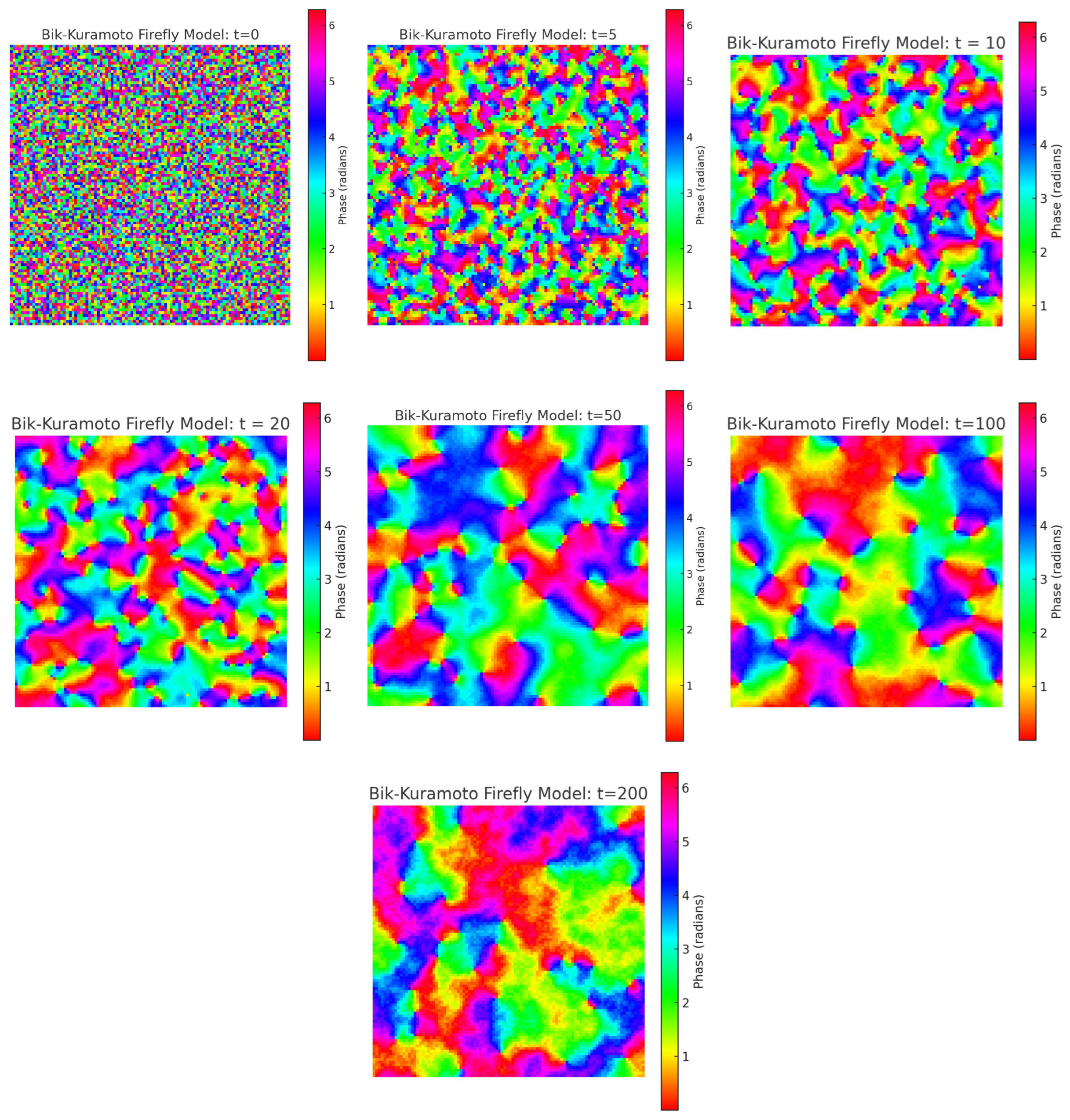
10. Bik-Kuramoto Firefly Model

10.1. Bik-Kuramoto Equation

We define the Bik-Kuramoto model as a discrete phase-coupled oscillator network evolving on a 2D grid:

$$E_{t}u=\left(u+w(x,y)+{\displaystyle \frac{K}{8}}\sum _{(i,j)\in M}sin(E_x^i{E}_y^{j}u-u)\right)mod2\pi$$

• $u=u(t,x,y)$ is the phase at grid point $(x,y)$ and time t.
• $w(x,y)$ is a fixed intrinsic frequency assigned randomly to each point.
• K is the coupling constant. In our simulations, we choose $K=1$.
• M is the Moore neighbourhood:

  $$M=\left\{\right(\pm 1,0),(0,\pm 1),(\pm 1,\pm 1\left)\right\}$$

10.2. Principle of Locality

In the original Kuramoto model, oscillators are globally coupled, each unit interacts with every other oscillator in the system. [6]. While this assumption simplifies mathematical analysis, it is biologically implausible. For example, it is unreasonable to assume that a firefly can perceive and compute the phases of all other fireflies in the environment at each time step.

To address this limitation, I propose the Bik-Kuramoto Firefly Model, which enforces the Principle of Locality. In this model, each oscillator interacts only with its immediate neighbors (e.g., a Moore neighborhood in two dimensions). This localized interaction is more consistent with real world biological systems and gives rise to rich emergent phenomena such as synchronization, topological defects, and vortex-like phase structures.

10.3. Observations and Phenomena

In the simulation, we use periodic boundary condition.

From the spatiotemporal plots of the system, we observe the following:

• The system exhibits topological defects: points around which the phase (color) continuously wraps from 0 to $2\pi$.
• These defects appear in pairs, with opposite rotational direction:

  –

  One clockwise

  –

  One counterclockwise

• When these defects move and eventually annihilate each other, a large region of synchronization emerges suddenly.

This model shows interesting connections to:

• Phase synchronization phenomena
• Topological vortex dynamics
• Pattern formation and self-organization

Figure 12. Spatiotemporal evolution of the Bik-Kuramoto model. Topological defects (vortices) emerge and move, and their annihilation leads to large-scale synchronization.

Figure 12. Spatiotemporal evolution of the Bik-Kuramoto model. Topological defects (vortices) emerge and move, and their annihilation leads to large-scale synchronization.

11. The Langton’s Ant

11.1. The Langton’s Ant Equations

We describe the classical Langton Ant using a System of Coupled Ordinary and Partial Difference Equations.

The update rules are given as follows:

$$\begin{array}{cc}\hfill u(t+1,x,y)& =u(t,x,y)+\left(1-2u(t,x,y)\right)·\delta (x-X\left(t\right))\delta (y-Y\left(t\right))\hfill \\ \hfill d(t+1)& =\left(d\left(t\right)+\left(1-2u(t,X(t),Y(t\left)\right)\right)\right)mod4\hfill \\ \hfill X(t+1)& =X\left(t\right)+cos\left({\displaystyle \frac{\pi }{2}}·d(t+1)\right)\hfill \\ \hfill Y(t+1)& =Y\left(t\right)-sin\left({\displaystyle \frac{\pi }{2}}·d(t+1)\right)\hfill \end{array}$$

Here, $\delta (x-X(t\left)\right)$ denotes the Kronecker delta function:

$$\delta (x-X\left(t\right))=\left\{\begin{array}{cc}1\hfill & \mathrm{if}x=X\left(t\right)\hfill \\ 0\hfill & \mathrm{otherwise}\hfill \end{array}\right.$$

This is a System of Coupled Ordinary and Partial Difference Equations.

11.2. Observations and Phenomena

The system exhibits transient chaos, followed by the emergence of a repeating structure called the highway, which acts as a periodic attractor in the phase space.

12. Advantages of Rewriting Complex Systems as Partial Difference Equations

12.1. Elegant and Unified Framework

Partial Difference Equations provide a universal and elegant mathematical language to describe a wide range of complex systems. Instead of relying on a fragmented set of ad hoc models, many seemingly unrelated systems can be encoded using the same formalism. This promotes unification across disciplines such as biology, physics, and computer science.

12.2. Mathematical Rigor and Analytical Tools

By expressing complex systems through Partial Difference Equations, we enable the use of powerful tools from modern mathematics, including functional analysis, topology, and chaos theory. This increases the precision, clarity, and theoretical strength of the analysis.

12.3. Extending Modeling Paradigms to Dynamic Models

Most existing models in complex systems theory are static or discrete-time without spatial dynamics. Partial Difference Equations allow for the natural inclusion of discrete vector fields and evolving spatial patterns. This opens the door to modeling dynamically evolving systems, including systems with multiple interacting fields, variables, and emergent behavior.

13. A Qualitative Study of the Edge of Chaos

In this framework, what is traditionally called the Edge of Chaos is rephrased and generalized as Quasichaos.

13.1. Definition of Periodic Islands

Choose a rectangle with minimum size $3\times 3$ covering a local region of the spatiotemporal grid governed by a partial difference equation (e.g., a cellular automaton). If the solution inside this rectangle satisfies the condition

$$u(t,x)=u(t+T,x+L)$$

for some integers $T,L$ not both zero, and exhibits at least three complete cycles, then we define this region as a periodic island.

13.2. Definition of Chaotic Sea

Likewise, consider a $3\times 3$ rectangle. If the solution within this region fails to satisfy any periodic relation, and is sensitive to initial conditions, we define this region as a chaotic sea.

13.3. Qualitative Definition of Quasichaos

While it is difficult to formalize a strict mathematical definition of quasichaos, here we offer a qualitative description based on observable dynamical traits. A system is said to exhibit quasichaos if the following conditions are met:

1.

Heterogeneous Distribution of Entropy

Quasichaotic systems exhibit spatial heterogeneity—regions of ordered, low-entropy structure coexist with disordered, high-entropy turbulence.

For example, in Rule 110:

• Some regions form stable, low-entropy periodic islands.
• Others exhibit turbulent, high-entropy chaotic seas.

This coexistence of local order and disorder is a hallmark of quasichaos.

2.

Multiscale Invariance

Regardless of observation scale, the system displays a self-similar hierarchy:

• Many small periodic islands;
• Fewer large ones.

The distribution likely follows a power-law, indicating scale-invariant structure.

3.

Turing Completeness

Most known quasichaotic systems (e.g., Rule 110, the Game of Life) are Turing-complete:

• They can simulate arbitrary logic or computation;
• Their visual complexity reflects true computational universality.

We conjecture that quasichaos lies at the interface of order and disorder, offering both structural richness and computational depth.

13.4. Definition of Quasichaotic System

We define that if a system exhibit Quasichaos, then we call the system as a Quasichaotic System.

14. Spacetime Modeling Paradigms

14.1. Partial Differential Equations on Manifolds

Partial Differential Equations (PDEs) can be formulated on various geometric structures. Here we present several examples based on different underlying manifolds.

PDE in Rectangular Coordinates

This is the most familiar case, where PDEs are defined over Euclidean space with Cartesian coordinates.

Example: 3D Kuramoto–Sivashinsky Equation

$${\displaystyle \frac{\partial u}{\partial t}}+{\nabla }^{4}u+{\nabla }^{2}u+{\displaystyle \frac{1}{2}}{(\nabla u)}^2=0$$

PDE in Spherical Coordinates

Spherical coordinates are used when the problem has spherical symmetry.

Example: 3D Heat Equation in Spherical Coordinates

$${\displaystyle \frac{\partial u}{\partial t}}=\alpha \left({\displaystyle \frac{1}{r^2}}{\displaystyle \frac{\partial }{\partial r}}\left(r^2{\displaystyle \frac{\partial u}{\partial r}}\right)+{\displaystyle \frac{1}{r^{2}sin\theta }}{\displaystyle \frac{\partial }{\partial \theta }}\left(sin\theta {\displaystyle \frac{\partial u}{\partial \theta }}\right)+{\displaystyle \frac{1}{r^2{sin}^2\theta }}{\displaystyle \frac{{\partial }^{2}u}{\partial {\varphi }^2}}\right)$$

PDE on Spherical Surface

When dynamics are constrained to the surface of a sphere, the Laplacian is replaced by the Laplace-Beltrami operator on the 2-sphere.

Example: Heat Diffusion on a Spherical Surface

$${\displaystyle \frac{\partial u}{\partial t}}={\Delta }_{{\mathbb{S}}^2}u$$

where ${\Delta }_{{\mathbb{S}}^2}$ is the Laplace-Beltrami operator on the sphere.

PDE on Lorentzian Manifold

These are relativistic field equations defined on a curved spacetime manifold with Lorentzian metric.

Example: Einstein Field Equations

$$R_{\mu \nu }-{\displaystyle \frac{1}{2}}R{g}_{\mu \nu }+\Lambda g_{\mu \nu }={\displaystyle \frac{8\pi G}{c^4}}{T}_{\mu \nu }$$

where $R_{\mu \nu }$ is the Ricci tensor, R is the Ricci scalar, $g_{\mu \nu }$ is the metric tensor, $\Lambda$ is the cosmological constant, and $T_{\mu \nu }$ is the energy-momentum tensor.

14.2. Partial Difference Equations on Networks

P$\Delta$E on Uniform Grids

Although in this paper, all the models and Partial Difference Equations are defined on square lattices, we note that other types of regular grids can also be used, such as triangular grids and hexagonal grids. These alternative lattices provide different topological and geometrical properties, which may influence the dynamics of the system.

P$\Delta$E in Other Coordinates

Beyond Cartesian grids, Partial Difference Equations can be extended to cylindrical or spherical coordinates. This allows us to model systems with rotational or radial symmetry, enabling a broader range of physical or biological simulations.

P$\Delta$E on Polyhedral Surfaces

Partial Difference Equations can also be defined on polyhedral surfaces. For example, we can construct cellular automata or discrete evolution rules on the surface of:

• Triangulated sphere
• Goldberg polyhedron
• Zonohedron

An example is the evolution of a cellular automaton on the surface of a Goldberg polyhedron, where the topology introduces curvature and complex connectivity into the system.

P$\Delta$E on Irregular Networks

In more general settings, Partial Difference Equations can be defined on irregular graphs or networks. These include:

• Random networks
• Scale-free networks
• Small-world networks

In such systems, individuals (nodes) are connected via irregular topologies, and their state evolution is determined by local interactions with neighbors. These models are powerful but difficult to analyze due to their topological complexity.

14.3. The Paradigms of Spacetime Modeling

We classify all dynamical systems based on the nature of time and space into four fundamental paradigms:

Table 1. Classification of Dynamical Modeling Paradigms Based on Time and Space

Paradigm	Time	Space	Typical Models
1	Continuous	Continuous	Partial Differential Equations (PDE); widely used in fluid dynamics, field theory, and continuum mechanics.
2	Discrete	Discrete	Partial Difference Equations (P$\Delta$E); cellular automata, sandpile models, forest fire models.
3	Continuous	Discrete	Ordinary Differential Equations (ODE) on networks; used in oscillator networks, epidemiology on graphs, neural dynamics.
4	Discrete	Continuous	Discrete-time maps on continuous manifolds; e.g., logistic maps with spatial extension, iterative geometric deformations.

Table 1. Classification of Dynamical Modeling Paradigms Based on Time and Space

Paradigm	Time	Space	Typical Models
1	Continuous	Continuous	Partial Differential Equations (PDE); widely used in fluid dynamics, field theory, and continuum mechanics.
2	Discrete	Discrete	Partial Difference Equations (P$\Delta$E); cellular automata, sandpile models, forest fire models.
3	Continuous	Discrete	Ordinary Differential Equations (ODE) on networks; used in oscillator networks, epidemiology on graphs, neural dynamics.
4	Discrete	Continuous	Discrete-time maps on continuous manifolds; e.g., logistic maps with spatial extension, iterative geometric deformations.

14.4. Continuous Space and Continuous Time

In this modeling paradigm, both space and time are treated as continuous variables. The natural mathematical framework for such systems is that of Partial Differential Equations (PDE). These equations describe how physical quantities vary over both time and spatial dimensions, and are fundamental in the study of continuous systems such as fluids, fields, and waves.

A canonical example is the Navier–Stokes equations, which govern the dynamics of incompressible fluid flow:

$${\displaystyle \frac{\partial \mathbf{u}}{\partial t}}+(\mathbf{u}·\nabla )\mathbf{u}=-\nabla p+\mu {\nabla }^2\mathbf{u}+\rho \mathbf{g},\nabla ·\mathbf{u}=0$$

(1)

Here, $\mathbf{u}(\mathbf{x},t)$ is the velocity field, p is the pressure, and $\nu$ is the kinematic viscosity. These equations capture the full spatiotemporal dynamics of fluid motion in a continuum.

This paradigm applies to a wide range of physical systems, including heat diffusion, wave propagation, electromagnetism, and general relativity. The underlying assumption is that the system can be described by smooth fields defined over a continuous domain in both space and time.

14.5. Discrete Space and Discrete Time

In this paradigm, both space and time are discretized. The natural mathematical formulation for such systems is via Partial Difference Equations (P$\Delta$E). These equations define the evolution of quantities on a lattice over discrete time steps. This framework is especially powerful for modeling cellular automata, reaction-diffusion processes on grids, and other discrete spatiotemporal dynamical system.

A representative example is the Abelian Sandpile Model, which is a prototypical system exhibiting self-organized criticality. Its update rule can be formulated as the following partial difference equation:

$$u(t+1,x,y)=u(t,x,y)-4·\theta (u(t,x,y)-4)+\sum _{(i,j)\in V}\theta (u(t,x+i,y+j)-4)+G(t,x,y)$$

(2)

Here:

• $u(t,x,y)$ is the number of sand grains at lattice site $(x,y)$ at time t;
• $\theta$ is the Heaviside step function, used to check if a site is unstable ($u\ge 4$);
• V is the neighborhood (e.g., the von Neumann neighborhood $\left\{\right(\pm 1,0),(0,\pm 1\left)\right\}$);
• $G(t,x,y)$ represents external grain addition (driving term).

This framework captures the discrete and rule-driven nature of systems like cellular automata and sandpile models. It is suitable for analyzing emergent complexity, self-organization, and critical phenomena arising from purely local interactions over discrete spacetime.

14.6. Discrete Space and Continuous Time

In this paradigm, space is discretized, often as a graph or lattice, while time remains continuous. This setup is naturally modeled using Ordinary Differential Equations (ODE) defined on graphs or networks, a common approach in systems biology, network dynamics, and synchronization phenomena.

A general form of such models can be expressed as:

$${\displaystyle \frac{\partial u}{\partial t}}=F\left(u(t,x,y,z),\mathcal{N}\left(u\right)\right)$$

(3)

where:

• $u=u(t,x,y,z)$ represents the state at discrete spatial position $(x,y,z)\in {\mathbb{Z}}^3$ and continuous time t;
• $\mathcal{N}\left(u\right)$ denotes the set of the neighbours;
• F is a function describing the local dynamics and interactions.

This framework bridges differential equations with network science. It is especially suitable for modeling dynamical processes such as neural activity, epidemic spreading, oscillator synchronization, and other time-evolving phenomena over discrete spatial structures.

14.7. Continuous Space and Discrete Time

In this paradigm, time is treated as discrete while space remains continuous. This modeling framework resembles discrete-time maps, but instead of operating on scalars or vectors, the input and output are functions defined over continuous space—such as curves or manifolds.

This paradigm is particularly useful for modeling processes where updates occur in discrete steps, but spatial continuity or smoothness is preserved at each step.

Example 1: Curve Shrinking in Discrete Time

$$u(t,x)={\displaystyle \frac{1}{t}}sin\left(x\right)$$

(4)

where $t\in \mathbb{Z}$ and $x\in \mathbb{R}$. This represents the evolution of a continuous curve where the amplitude shrinks over discrete time steps.

Example 2: Shrinking Circle

$$\mathbf{r}(t,\theta )=\left(x(t,\theta ),y(t,\theta )\right)=\left({\displaystyle \frac{1}{t}}cos\theta ,{\displaystyle \frac{1}{t}}sin\theta \right)$$

(5)

where $t\in \mathbb{Z}$ and $\theta \in \mathbb{R}$. This describes a shrinking circle in ${\mathbb{R}}^2$ as time progresses in discrete steps.

This paradigm opens the door to novel formulations where dynamical rules act on spatially continuous fields in discrete temporal slices, bridging discrete dynamical systems with continuous geometry.

15. Summary

In this paper, we initiate a systematic study of Partial Difference Equations (P$\Delta$E) as a mathematical framework for modeling discrete dynamical systems across space and time. We begin by defining the structure and classification of P$\Delta$E, including autonomous and non-autonomous types, and derive exact solutions to several linear cases using discrete Hilbert spaces, operator theory, and discrete Green’s functions.

We then unify a wide range of well-known complex systems—including 1D Cellular Automata, Conway’s Game of Life, the Abelian Sandpile Model, Langton’s Ant, Forest Fire Models, Firefly Synchronization, and the OFC Earthquake Model, by rewriting them in the form of nonlinear P$\Delta$E. This provides a powerful language for analyzing initial conditions, boundary conditions, and perturbations within a single formal system.

A novel concept called quasichaos is introduced to generalize the notion of "edge of chaos," capturing systems that exhibit a mixture of periodicity, disorder, and self-organized complexity. Quasichaotic patterns are characterized by features such as spatially non-uniform structures, power-law distributions, computational universality, and emergent modularity.

Finally, we explore the formulation of P$\Delta$E on more general topologies, including hexagonal grids, irregular networks, and polyhedral surfaces, drawing parallels with PDE on manifolds. We classify four modeling paradigms: discrete space-time, continuous space-time, continuous-time on discrete space, and discrete-time on continuous space.

This work is intended not as a declaration, but as an invitation, to reimagine the foundations of biological and physical modeling through the language of P$\Delta$E.

References

- Elaydi, S. An Introduction to Difference Equations, 3rd ed.; Undergraduate Texts in Mathematics, Springer: New York, 2005. [Google Scholar]
- Olver, P.J. Introduction to Partial Differential Equations; Undergraduate Texts in Mathematics, Springer: Cham, Heidelberg, New York, Dordrecht, London, 2014. [Google Scholar] [CrossRef]
- Wolfram, S. A New Kind of Science, 1st ed.; Wolfram Media: Champaign, Illinois, 2002. [Google Scholar]
- Itoh, M.; Chua, L.O. Difference Equations for Cellular Automata. International Journal of Bifurcation and Chaos 2009, 19, 805–830. [Google Scholar] [CrossRef]
- Bak, P.; Tang, C.; Wiesenfeld, K. Self-Organized Criticality: An Explanation of 1/f Noise. Physical Review Letters 1987, 59, 381–384. [Google Scholar] [CrossRef] [PubMed]
- Strogatz, S.H. From Kuramoto to Crawford: Exploring the Onset of Synchronization in Populations of Coupled Oscillators. Physica D: Nonlinear Phenomena 2000, 143, 1–20. [Google Scholar] [CrossRef]
Disclaimer/Publisher’s Note: The statements, opinions and data contained in all publications are solely those of the individual author(s) and contributor(s) and not of MDPI and/or the editor(s). MDPI and/or the editor(s) disclaim responsibility for any injury to people or property resulting from any ideas, methods, instructions or products referred to in the content. |
© 2025 by the authors. Licensee MDPI, Basel, Switzerland. This article is an open access article distributed under the terms and conditions of the Creative Commons Attribution (CC BY) license (http://creativecommons.org/licenses/by/4.0/).
Copyright: This open access article is published under a Creative Commons CC BY 4.0 license, which permit the free download, distribution, and reuse, provided that the author and preprint are cited in any reuse.