Submitted:
10 July 2025
Posted:
10 July 2025
You are already at the latest version
Abstract
A rotating imperfect ring resonator in a gyroscope is modeled by a rotating thin ring with evenly distributed point masses. The free response of the rotating ring structure at constant speed is investigated, including the steady elastic deformation and wave response. The dynamic equations are formulated by using Hamilton's principle in the ground-fixed coordinates. The coordinate transformation is applied to facilitate the solution of the steady deformation, and the displacements and tangential tension for the deformation are calculated by the perturbation method. Employing the Galerkin’s method, the governing equation of the free vibration is cast in matrix differential operator form after the separation of the real and imaginary parts with the inextensional assumption. The natural frequencies are calculated through the eigenvalue analysis and the numerical results are obtained. The effects of the point masses on the natural frequencies of the forward and backward traveling wave curves of different orders are discussed, especially on the measurement accuracy of gyroscopes for different cases. In the ground-fixed coordinates, the frequency splitting results in a crosspoint of the natural frequencies of the forward and backward traveling waves. The finite element method is applied to demonstrate the validity and accuracy of the model.
Keywords:
ring resonator
; mass imperfections
; steady elastic deformation
; traveling waves
; natural frequencies
1. Introduction
Frequency-modulated gyroscope is a high-precision angular rate sensor with the advantages of low power consumption, low temperature sensitivity, high bandwidth, and excellent scale factor stability. The core working element of a frequency-modulated gyroscope is the resonator, and the thin ring is one of the most commonly employed resonators in practical applications due to the simple structure and stability [1,2].
The ring-shaped structures have attracted great attentions since they are widely applied in rate sensors, gears, electric motors and ultrasonic motors, etc., owing to their axial symmetry and excellent mechanical properties [3,4,5,6]. In general, the free response of the stationary ring is standing waves or the real modes, while that of the rotating ring is traveling waves or the complex modes. The resonant ring of the gyroscope works in a rotating state and its free response is traveling waves due to the Coriolis effect. The investigations on the dynamics of the perfect rings and stationary imperfect rings are sufficient, such as the research on the problems of natural frequencies [7,8,9], mode contaminations [10], wave propagations [11,12], quality-factors [13], nonlinearities [14,15] and stabilities [16,17,18]. Meanwhile, the studies on rotating rings with non-uniform mass or density distribution is relatively fewer.
For stationary perfect rings, except the rigid body modes, it has elastic breathing mode, pairs of degenerate bending modes with nth orders (integer n>1), and pairs of longitudinal modes with much higher natural frequencies [7,19]. If the symmetry of the ring is broken by imperfections, the natural frequencies of bending mode pair with certain orders can split due to the non-uniform mass or stiffness distribution [10]. For rotating perfect rings, the free response for each order are two traveling waves with branched frequencies because of the Coriolis effect [8,9]. Frequency-modulated gyroscopes measure angular rate by the frequency difference between two traveling waves. The non-linear phenomenon can be aroused by the electrostatic force for the rotating ring subjected to non-uniform electric field [17] or the geometric non-linearity is considered [15]. Also, parametric instabilities can result from the time-varying rotating speed [16] or structure eccentricity [20].
For rotating rings with imperfections, Kim et al. [21] analyzed the thermoelastic effect on the rotating ring with non-uniform density under the in-extensional assumption, and the frequency expression included the variable density. The longitude deformation along the rotating ring is ignored in most research since it is really small especially for low-speed condition [22,23]. Nevertheless, the transverse deformation due to imperfections is better to be considered because it is on a larger scale than the longitudinal one and leads to variation of the normal stress, which can even cause parametrical instability for varying speed condition.
The mathematic model of the rotating ring can be established in ground-fixed coordinates or body-fixed coordinates. By using Hamilton’s principle, the effect of circumferential stress on strain energy is directly involved if the energies are calculated in the ground-fixed coordinates [11,12], whereas the strain energy caused by the centrifugal force needs to be considered separately if it is modeled in the body-fixed coordinates [9].A similar problem is explored by Zhang et al. [24] in the ring-fixed coordinate, and the frequency splitting phenomenon cannot be observed by setting the speed to be zero in the model of rotating ring.
From a practical point of view, it is difficult to eliminate factors such as machining errors and uneven materials in a small mechanical part and the mass imperfections on the resonant ring in a gyroscope are inevitable [13,21]. Thus, it is essential to investigate the influence of mass imperfections on the vibration characteristics of the ring resonator. This work considers the ring resonator of the frequency-modulated gyroscope where the mass imperfections are evenly distributed, aiming to provide a more accurate analysis for the rotating thin ring structure with equally spaced mass imperfections. The results can lay the foundation for further research, for instance, on the effects of variable rotating speed, the nonlinearities from the large deformation and the free response of resonant ring with random mass imperfections. The numerical results of the natural frequencies are compared with those obtained from the finite element method, demonstrating the validity and accuracy of the present work.
2. Dynamic Modeling
2.1. Model Description
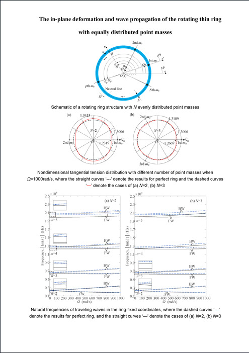
Figure 1 presents the rotating ring resonator model in a gyroscope with mass imperfections, where O-rθz is the ground-fixed coordinates and O-r′Θz is the ring-fixed coordinates. The origin O is located at the geometric center and z-axis is pointing out of the paper. The polar axes of the two coordinates coincide at the initial moment. To facilitate further investigation into the free response of the rotating resonant ring with random mass imperfections, this study analyzes the case in which the mass imperfections are evenly distributed. Mass imperfections are represented by point masses in dynamic model. N is the number of point masses, m0 is the point mass, p is the ordinal number of the point masses, R is the neutral circle radius and b is the axial height, h is the radial thickness which is much smaller than the neutral circle radius, satisfying the thin ring assumption, ρ, E, and Ω are the material density, Young’s modulus, and rotational speed, respectively.
The u(θ, t) and v(θ, t) are the tangential and radial displacements of any point on the neutral circle in the ground-fixed coordinates, respectively, which are functions of angle θ and time t.
2.2. Equations of Motion
The dynamic model is established in the ground-fixed coordinates, and the Dirac function is employed to represent the linear density of the point masses:
where δ is the Dirac function and k is an integer to ensure that
The ring is treated as the Euler–Bernoulli beam and the energy method is to be utilized. The displacement vector of any point (R, θ) on the neutral circle is
where er and eθ are the radial and tangential unit vectors.
The velocity is determined by the time derivative of the position vector:
The cross-section taken normal to the middle surface of the ring remains normal after deformation. Neglecting the rotary inertia effects, the kinetic energy can be expressed as
where A (A=bh) is the cross-sectional area.
The tangential strain anywhere on the cross-section of the ring [12] is
According to Eq.(5), the tangential strain of an arbitrary point on the neutral circle is given by
In the ground-fixed coordinates, the normal stress of the cross-section is not needed to be calculated separately for the potential energy caused by the centrifugal tension [12], not like the analysis in Ref. [9]. The constitutive equation used in this work is Hooke’s Law, that is, the stress σ equals to Eεθ. Then the strain energy is
Assuming that the vibration amplitude and the deformation are minimal, the high terms in the strain energy is neglected. Substitution of the strain in Eq. (5) into the strain energy and simplification gives
The Hamilton’s principle is employed
Substituting Eqs. (4) and (8) into Eq. (9), yields the partial differential equations for v and u:
where θp=2π(p-1)/N+Ωt.
3. Model Analysis
3.1. Solution Strategy
In the ground-fixed coordinates, the partial differential dynamical equations of the model contain time-varying coefficients, making them challenging to solve. For the purpose of the calculation of the steady elastic deformation and nature frequencies, the model is converted into the ring-fixed coordinates through coordinate transformation θ=Θ+Ωt. The µ(Θ, t) and υ(Θ, t) are used to represent the corresponding tangential and radial displacements in the ring-fixed coordinates. The partial differential dynamical equations for µ and υ are
where Θp=2π(p-1)/N.
The partial differential dynamic equations for µ and υ are time-invariant coefficients, and the characteristics of the modes can be solved through the eigenvalue analysis.
The ring resonator in a gyroscope is assumed to be extensible with the centrifugal effect at the rotational speed Ω, and to be inextensible during the micro bending vibration based on the steady deformation. The radial and tangential displacements on the neutral circle can be expressed as
where υfinal and µfinal are the total radial and tangential displacements, υe and µe are the radial and tangential displacements of the steady elastic deformation, υ and µ are the radial and tangential displacements for the inextensible vibration, respectively.
3.2. Steady Elastic Deformation
Due to the influence of the mass imperfections, the shape of the steady elastic deformation is not circular but a rotationally symmetric shape with an angular period related to the number of mass imperfections N. The steady elastic deformation of the model can be approximated as the superposition of the steady elastic deformation of a perfect rotating resonant ring in a gyroscope and the deformation induced by the influence of mass imperfections. The radial and tangential displacements on the neutral circle are independent of time t and depend on the angle Θ. Correspondingly, the radial and tangential displacements on the neutral circle are expressed as perturbation form
where υe0 and µe0 are the radial and tangential displacements of a perfect rotating ring, υe1 and µe1 are the additional radial and tangential displacements induced by the influence of the mass imperfections, respectively. εm0 is a small parameter, indicating the degree of influence exerted by the mass imperfections on the rotating ring, and εm0=m0/ρAR.
Substituting Eqs. (14a) and (14b) into Eqs. (12) and (13). For moderate speeds and stiff rings, the extensional deformation during rotation is small, the nonlinear terms in the equations can be neglected. The partial differential equations for υe and µe are
Substituting Eqs. (7a) and (8b) into Eqs. (16) and (17), and separating the equations by orders of εm0, yields
Due to the periodicity of the radial and tangential displacements with respect to the angle Θ, they are expressed in the form of Fourier series as
Substituting Eqs. (22a) and (22b) into Eqs. (20) and (21), there are
According to Eqs. (15a), (15b), (23) and (24), the radial and tangential displacements on the neutral circle are
where α=E/ρR2Ω2, β=Eh2/12ρR4Ω2, φ(j)=αβj6-(2αβ+β)j4-(α+β-αβ)j2+1-α.
Table 1 shows the basic parameters of the model. The thickness of the ring resonator is much smaller than the radius of the neutral circle, satisfying the thin ring assumption.
Figure 2 exhibits the displacements of the points on the neutral circle for steady elastic deformation. The red and blue lines mean the radial and tangential displacements, respectively. Figure3 shows the steady elastic deformation diagrams obtained from Eq. (25).
It is shown that the radial and tangential displacements are periodic with respect to the angle Θ, and the angular period is 2π/N. Both the amplitudes of the radial and tangential displacements decrease as the number of mass imperfection increases, and the radial displacement gradually becomes the dominant component of the steady elastic deformation.
The maximum radial displacement occurs at the locations of mass imperfection (Θ=2π(p-1)/N), while the minimum radial displacement occurs at the midpoints between two adjacent mass imperfection (Θ=π(2p-1)/N). At both the locations, the tangential displacement is zero. The maximum tangential displacement occurs at angles πp/2N and 3πp/2N, where the magnitudes are equal but the directions are opposite. At the maximum tangential displacement, the radial displacement equals υe0, which corresponds to the radial displacement of a perfect rotating ring. This indicates that at the maximum tangential displacement, the influence of the mass imperfections on the radial displacement is negligible.
According to Eq. (6), for moderate speeds and stiff rings, the extensional deformation during rotation is small and the quadratic term can be neglected. The tangential strain on the neutral circle is
Then the tangential tension on the neutral circle is
in which the tangential tension is divided into two components, the NΘ1 equaling to the tension of the perfect rotating ring and the additional part NΘ2 affected by the mass imperfections
The strain follows the same trend as the tangential tension, and it is sufficient to analyze one of them. Figure 4 provides the nondimensional tangential tension on the neutral circle with different numbers of mass imperfections based on the parameters in Table 1, where =NΘR2/EI and I=Ah2/12. It can be observed that the presence of evenly distributed mass imperfections leads to a redistribution of tangential tension in the rotating ring by comparing the tangential tension distribution without mass imperfections. Specifically, the angular period of the tangential tension distribution with evenly distributed mass imperfections is 2π/N.
In Figure 4, the tangential tension is minimal at the mass imperfection locations and maximal midway between adjacent mass imperfections. The maximum tangential tension decreases with increasing N. According to Eq. (27), the total tangential tension is related to the radial displacement υe and the rate of change of tangential displacement ∂µe/∂Θ. The tangential tension EAυe0/R of the perfect rotating resonant ring is a constant value determined by υe0. The additional tangential tension caused by the mass imperfections is mainly related to ∂µe/∂Θ. At the mass imperfection locations, although the radial displacement υe reaches its maximum, υe0 remains constant and ∂µe/∂Θ is minimal, resulting in both the additional tangential tension and the total tangential tension being minimized.
For the tangential tension EAυe0/R of the perfect rotating ring, the radial displacement υe0 in Eq. (23) becomes extremely large as the rotational speed approaches . The elastic force of the rotating ring is difficult to balance the centripetal acceleration, leading to unsteady deformation. We restrict the model’s rotational speed to below . According to the basic parameters given in Table 1, this speed is approximately 50,000 rad/s.
For the additional tangential tension caused by the mass imperfections, the tangential tension NΘ in Eq. (23) becomes extremely large as φ(j) approaches zero. The rotational speed corresponding to φ(j)=0 is the speed at which the deformation becomes unsteady. Figure 5 depicts the variation of φ(j) with respect to the rotational speed, considering only the cases below rotational speed .
Figure 5 shows that the rotational speed corresponding to φ(j)=0 becomes higher with an increasing N. For a given number of mass imperfections, the rotational speed corresponding to φ(j)=0 is minimal. When N=8, the rotational speed corresponding to φ(j)=0 exceeds . The rotational speed at which the deformation becomes unsteady does not need to be considered during medium and low-speed rotations. Increasing the number of evenly distributed mass imperfections can enhance the stability of the steady elastic deformation of the ring resonator of gyroscope.
3.3. Free Response
The ring resonator of the gyroscope is assumed to be inextensional for the flexural vibration, based on the stretched configuration considering centrifugal effect. Therefore, the inextensional assumption [25] can be applied:
The radial and tangential displacements vary with time t during vibration. Substituting Eqs. (14a) and (14b) into Eqs. (12) and (13), eliminating the constant and nonlinear terms, the system of partial differential equations describing the model’s vibration is
Substituting Eqs. (27) and (28) into Eqs. (29) and (30), the vibrational partial differential equation for the tangential displacement µ(Θ, t) is
By using the Galerkin’s method, the tangential displacement µ(Θ, t) is written as
where qn(t) is a complex function of the time t, n is vibration wavenumber, i () is the imaginary unit, and “~” designates the complex conjugate operation.
To facilitate analysis, the complex function qn(t) is rewritten as
where x(t) and y(t) are both real functions of the time.
Defining an inner product as
Substituting Eqs. (32) and (33) into Eq (31), forming the inner product with einΘ, the real and imaginary parts can be separated. Two cases are considered based on different relationships of n and N.
Case Ι: 2n/N=int
The governing equation in matrix differential operator form is
Where
Equation (35) is the kinetic equation with constant coefficient, and the characteristics of the mode can be obtained through the eigenvalue analysis of the system. The state vector is
Substituting Eq. (36) into Eq. (35) gives
where is the state space matrix, and represent the zero matrix and the identity matrix, respectively.
Assuming ψ(t)=eλty, where λ is the eigenvalue of the system and y is the eigenvector. The characteristic equation is
According to the characteristic equation of the system, the equation for the eigenvalue λ can be expressed as
Where
Thus, the eigenvalues are
Assuming λ=λRe+iλIm, the real values λRe and λIm representing the real and imaginary parts of the eigenvalues, respectively. The eigenvalues for different conditions are summarized in Table 2.
Case ΙΙ: 2n/N≠int
The governing equation in matrix differential operator form is
Where
The corresponding characteristic equation is
The equation for the eigenvalue λ is
Where
The eigenvalues can be obtained from the Eq. (43)
Substituting λ=λRe+iλIm into Eq. (44), the eigenvalues are calculated and summarized in Table 3 for different conditions.
3.4. Qualitative Explanation of the Coriolis Effect
In fact, the literatures have explained the Coriolis effect on the phenomenon that the forward and backward waves travel with different speeds on the rotating ring by the analytical and numerical results clearly, whereas a qualitative illustration is still added here, which may be useful for the intuitive understanding.
Each point on the neutral plane moves along an elliptical trajectory when the ring rotates since the tangential and radial displacements are u=Ancos(nθ+ωnt) and v=nAnsin(nθ+ωnt), where An is vibration amplitude and ωn is natural frequency. The tangential and radial displacements satisfy u2+v2/n2=1, which corresponds to the ellipse.
The negative and positive natural frequencies correspond to the forward and backward waves, respectively. The clockwise of the motion of a point is present in Figure 6.
For the ground-fixed coordinates, the Coriolis effect should be analyzed based on the Coriolis force which can be judged by the right-hand rule. In this figure the Coriolis forces have the same direction with the displacement, and thus the forward wave is accelerated just like the stiffness has increased, and the opposite is true for the backward wave. Therefore, the forward wave travels faster seen in the ground-fixed coordinates.
While for the body-fixed coordinates, the Coriolis effect can be analyzed based on the Coriolis acceleration which is in opposite direction to the Coriolis force. Then the result is the backward wave travels faster or the frequency of backward wave is higher.
4. Numerical Results
4.1. Nature Frequencies and the Validation
The eigenvalues with parameters in Table 1 are computed numerically from the characteristic equation. The imaginary part of the eigenvalues represents the natural frequencies of the free vibration in the ring-fixed coordinates. The natural frequencies for varying rotational speeds are shown in Figure 7, with the abscissa representing the rotational speeds and the ordinate representing the natural frequencies of forward traveling waves (FW) and backward traveling waves (BW).
As shown in Figure 7, the natural frequencies of the rotating ring resonator with evenly distributed mass imperfections are lower than those of the perfect rotating ring at the same wavenumber n. The natural frequencies will be reduced by mass imperfections, with forward waves exhibiting a greater decrease than backward waves. In addition, the natural frequencies decrease with increasing N when the combinations of n and N belong to the same case (Ι or ΙΙ). Different relationships of n and N influence the natural frequency splitting at zero rotational speed. When 2n/N=int, the natural frequencies split. Specifically, the natural frequency of the BW of the rotating ring corresponds to the higher one of the split frequencies in the stationary state, and the natural frequency of the FW corresponds to the lower one. When 2n/N≠int, the natural frequencies do not split. The natural frequencies for a given wavenumber n of backward waves are greater than those of forward waves due to the Coriolis acceleration.
The finite element method (FEM) is applied to verify the numerical results by using the COMSOL Multiphysics software, taking N=4 as an illustrative example. The basic parameters in Table 1 are used for the simulation model. The physics interface selects the Solid Rotor (rotsld) in the Rotordynamics Module. This interface models the equations of motion for an observer sitting in a corotating frame of reference. Therefore, the natural frequencies solved by the finite element method are in the ring-fixed coordinates. The Coriolis and prestress effects are applied by setting the rotational speed. Table 4 gives the comparisons of natural frequencies (N=4) obtained by finite element method and numerical calculation.
The numerically calculated natural frequencies are circular frequencies ω (rad/s), and the frequencies in Table 4 are obtained by transforming f=ω/2π (Hz). The natural frequencies of the backward waves and forward waves are represented by fBW and fFW, respectively. Various rotational speeds are selected in the comparisons. It can be seen from Table 4 that the differences of the frequencies are small, and the maximal difference is less than 5%, which indicates the validity and accuracy of the model and approach.
Fully differential frequency-modulated gyroscopes measure the rotational speed based on the frequency difference between FW and BW by the Coriolis force. The frequencies of two modes have the same temperature dependency, and the frequency fluctuation induced by temperature can be cancelled out for the frequency difference, resulting in excellent temperature stability [26,27,28]. The eigenfrequenies of two modes are given as , where f0, k and Ω are natural frequency in the stationary state, scale factor and rotational speed, respectively.
There is an excellent linearity between the applied rotational speed and the frequency difference of two modes for perfect ring. Figure 8 shows the frequency difference between FW and BW based on parameters in Table 1.
When 2n/N=int, mass imperfections induce a significant discrepancy in the frequency difference between FW and BW of the imperfect and perfect resonant rings, especially in the low-speed range. This means that mass imperfections introduce a non-negligible error in rotational speed measurements in case Ι (2n/N=int). Furthermore, in the low-speed range, the mass imperfections also change the linearity between the frequency difference and the rotational speed. When 2n/N≠int, the frequency difference between FW and BW is nearly identical in both the imperfect and perfect rings, and the frequency-modulated gyroscope maintains high accuracy in rotational speed measurement.
4.2. Crosspoints of the Natural Frequencies of FW and BW
According to the Doppler effect, when converting the natural frequencies from the ring-fixed coordinates to the ground-fixed coordinates, the natural frequencies of forward waves increase by nΩ, whereas those of backward waves decrease by nΩ. Figure 9 shows the natural frequencies for varying rotational speeds in the ground-fixed coordinates.
In the ground-fixed coordinates, the natural frequencies of backward waves are always lower than those of forward waves for a given wavenumber n when 2n/N≠int. However, the situation of the natural frequencies is reversed between the high-speed and low-speed ranges when 2n/N=int. The frequency splitting causes the natural frequencies of backward waves to be higher than those of forward waves at zero rotational speed. In the low-speed range, the Doppler effect is not significant due to the low value of nΩ, and the natural frequencies of backward waves remain higher than those of forward waves because of the frequency splitting. As the rotational speed increases, the natural frequencies of forward waves gradually exceed that of backward waves. The transition in the magnitude relationship between the natural frequencies of forward and backward waves results in a crosspoint where their natural frequencies equal to each other.
Figure 10 shows the variation of rotational speeds and natural frequencies at the crosspoints due to the increase of the magnitude of the mass imperfection.
Variation curves of wavenumbers n=2, 4 and 6 are considered in Figure 10. Increasing the magnitude of the mass imperfection increases the rotational speeds at the crosspoints, while the natural frequencies exhibit an opposite trend. For the determined magnitude of the mass imperfection, larger values of N and n result in increased rotational speeds and natural frequencies at the crosspoints. When the magnitude of the mass imperfection approaches zero, the rotational speeds at the crosspoints also approach zero, since the natural frequencies of the perfect ring do not split in the stationary state.
5. Conclusions
This work derives a dynamic model for a rotating ring-shaped resonator in a gyroscope with evenly distributed mass imperfections, and the point masses are used to represent the mass imperfections. The effects of the evenly distributed mass imperfections on the steady elastic deformation and natural frequencies are investigated. Main conclusions are summarized below:
(1) The angular period of the displacements and tangential tension for the steady elastic deformation is 2π/N, and both the amplitudes of the displacements and tangential tension decrease with increasing N. There are multiple rotational speeds at which the deformation is unstable due to the mass imperfections. Increasing the number of evenly distributed mass imperfections can enhance the stability of the steady elastic deformation of the rotating ring.
(2) The natural frequencies of the stationary resonant ring split for integer 2n/N or remain degenerate for non-integer. The frequency splitting results in crosspoints of the natural frequencies of the FW and BW, and the magnitude of the mass imperfection can influence the rotational speeds and the natural frequencies at crosspoints. When 2n/N=int, the natural frequency of the BW of the rotating ring begins with the higher one of the split frequencies in the stationary state, and the natural frequency of the FW begins with the lower one.
(3) The mass imperfections reduce the natural frequencies of the rotating resonant ring in a gyroscope. When 2n/N=int, the mass imperfections will induce a significant discrepancy in the frequency difference between FW and BW of the imperfect and perfect rings, bringing a non-negligible error to frequency-modulated gyroscope. When 2n/N≠int, the frequency difference between FW and BW is nearly identical in both the imperfect and perfect rings. The comparison of natural frequencies obtained from the finite element method and numerical calculation reveals a maximum discrepancy of less than 5%.
Funding
This research was funded by the Basic Research Funds for National University, grant number 3122018D038, and the National Natural Science Foundation of China, grant number 51705519.
Conflicts of Interest
The authors declare no conflicts of interest.
References
- Li, R.; Wang, X.; Yan, K.; Chen, Z.; Ma, Z.; Wang, X.; Zhang, A.; Lu, Q. Interactive Errors Analysis and Scale Factor Nonlinearity Reduction Methods for Lissajous Frequency Modulated MEMS Gyroscope. Sensors 2023, 23, 9701. [Google Scholar] [CrossRef] [PubMed]
- Xing, J.R.; Xin, Z.; Sheng, Y.; Xue, Z.W.; Ding, B.X. Frequency-Modulated MEMS Gyroscopes: A Review. IEEE Sens. J. 2021, 21, 26426–26446. [Google Scholar]
- Wu, X.; Parker, R.G. Modal Properties of Planetary Gears With an Elastic Continuum Ring Gear. J. Appl. Mech. 2008, 75, 031014. [Google Scholar] [CrossRef]
- Liu, J.; Wang, S.; Wang, Z. Elimination of Magnetically Induced Vibration Instability of Ring-Shaped Stator of PM Motors by Mirror-Symmetric Magnets. J. Vib. Eng. Technol. 2019, 8, 695–711. [Google Scholar] [CrossRef]
- Yoon, S.W.; Lee, S.; Najafi, K. Vibration sensitivity analysis of MEMS vibratory ring gyroscopes. Sensors Actuators A: Phys. 2011, 171, 163–177. [Google Scholar] [CrossRef]
- Shi, S.; Xiong, H.; Liu, Y.; Chen, W.; Liu, J. A ring-type multi-DOF ultrasonic motor with four feet driving consistently. Ultrasonics 2017, 76, 234–244. [Google Scholar] [CrossRef]
- Soedel, W. Vibrations of Shells and Plates; Marcel Dekker: New York, NY, USA, 2004; ISBN 9780429216275. [Google Scholar]
- Kim, W.; Chung, J. FREE NON-LINEAR VIBRATION OF A ROTATING THIN RING WITH THE IN-PLANE AND OUT-OF-PLANE MOTIONS. J. Sound Vib. 2002, 258, 167–178. [Google Scholar] [CrossRef]
- Huang, S.; Soedel, W. Effects of coriolis acceleration on the free and forced in-plane vibrations of rotating rings on elastic foundation. J. Sound Vib. 1987, 115, 253–274. [Google Scholar] [CrossRef]
- Wang, S.; Xiu, J.; Gu, J.; Xu, J.; Liu, J.; Shen, Z. Prediction and suppression of inconsistent natural frequency and mode coupling of a cylindrical ultrasonic stator. Proc. Inst. Mech. Eng. Part C: J. Mech. Eng. Sci. 2010, 224, 1853–1862. [Google Scholar] [CrossRef]
- Huang, D.; Tang, L.; Cao, R. Free vibration analysis of planar rotating rings by wave propagation. J. Sound Vib. 2013, 332, 4979–4997. [Google Scholar] [CrossRef]
- Cooley, C.G.; Parker, R.G. Vibration of high-speed rotating rings coupled to space-fixed stiffnesses. J. Sound Vib. 2014, 333, 2631–2648. [Google Scholar] [CrossRef]
- Kim, J.-H.; Kang, S.-J. Splitting of quality factors for micro-ring with arbitrary point masses. J. Sound Vib. 2017, 395, 317–327. [Google Scholar] [CrossRef]
- Liang, F.; Liang, D.-D.; Qian, Y.-J. Nonlinear Performance of MEMS Vibratory Ring Gyroscope. Acta Mech. Solida Sin. 2020, 34, 65–78. [Google Scholar] [CrossRef]
- Yu, T.; Kou, J.; Hu, Y.-C. Vibration of a Rotating Micro-Ring under Electrical Field Based on Inextensible Approximation. Sensors 2018, 18, 2044. [Google Scholar] [CrossRef]
- Asokanthan, S.F.; Cho, J. Dynamic stability of ring-based angular rate sensors. J. Sound Vib. 2006, 295, 571–583. [Google Scholar] [CrossRef]
- Yu, T.; Kou, J.G.; Hu, Y.C. Vibrations of Rotating Ring Under Electric Field. J. Chin. Soc. Mech. Eng. 2021, 42, 51–62. [Google Scholar]
- Polunin, P.M.; Shaw, S.W. Self-induced parametric amplification in ring resonating gyroscopes. Int. J. Non-linear Mech. 2017, 94, 300–308. [Google Scholar] [CrossRef]
- Cooley, C.G.; Parker, R.G. Limitations of an inextensible model for the vibration of high-speed rotating elastic rings with attached space-fixed discrete stiffnesses. Eur. J. Mech. - A/Solids 2015, 54, 187–197. [Google Scholar] [CrossRef]
- Wei, Z.; Wang, S.; Wang, Y. Dynamic instability of an eccentrically rotating ring-shaped structure. Proc. Inst. Mech. Eng. Part C: J. Mech. Eng. Sci. 2024, 238, 4944–4958. [Google Scholar] [CrossRef]
- Kim, J.-H. Thermoelastic dissipation of rotating imperfect micro-ring model. Int. J. Mech. Sci. 2016, 119, 303–309. [Google Scholar] [CrossRef]
- Beli, D.; Silva, P.B.; Arruda, J.R.d.F. Vibration Analysis of Flexible Rotating Rings Using a Spectral Element Formulation. J. Vib. Acoust. 2015, 137, 041003. [Google Scholar] [CrossRef]
- Canchi, S.V.; Parker, R.G. Parametric Instability of a Rotating Circular Ring With Moving, Time-Varying Springs. J. Vib. Acoust. 2005, 128, 231–243. [Google Scholar] [CrossRef]
- Zhang, D.; Wang, S.; Liu, J. Analytical Prediction for Free Response of Rotationally Ring-Shaped Periodic Structures. J. Vib. Acoust. 2014, 136, 041016. [Google Scholar] [CrossRef]
- Charnley, T.; Perrin, R.; Mohanan, V.; Banu, H. Vibrations of thin rings of rectangular cross-section. J. Sound Vib. 1989, 134, 455–488. [Google Scholar] [CrossRef]
- Tsukamoto, T.; Tanaka, S. Fully Differential Single Resonator FM Gyroscope Using CW/CCW Mode Separator. J. Microelectromechanical Syst. 2018, 27, 985–994. [Google Scholar] [CrossRef]
- Tsukamoto, T.; Tanaka, S. Fully Differential Single Resonator FM Gyroscope Using CW/CCW Mode Separator. J. Microelectromechanical Syst. 2018, 27, 985–994. [Google Scholar] [CrossRef]
- Tsukamoto, T.; Tanaka, S. FM/rate integrating MEMS gyroscope using independently controlled CW/CCW mode oscillations on a single resonator. 2017 IEEE International Symposium on Inertial Sensors and Systems (INERTIAL); pp. 1–4.
Figure 1.
Schematic of a rotating ring structure with N evenly distributed point masses.
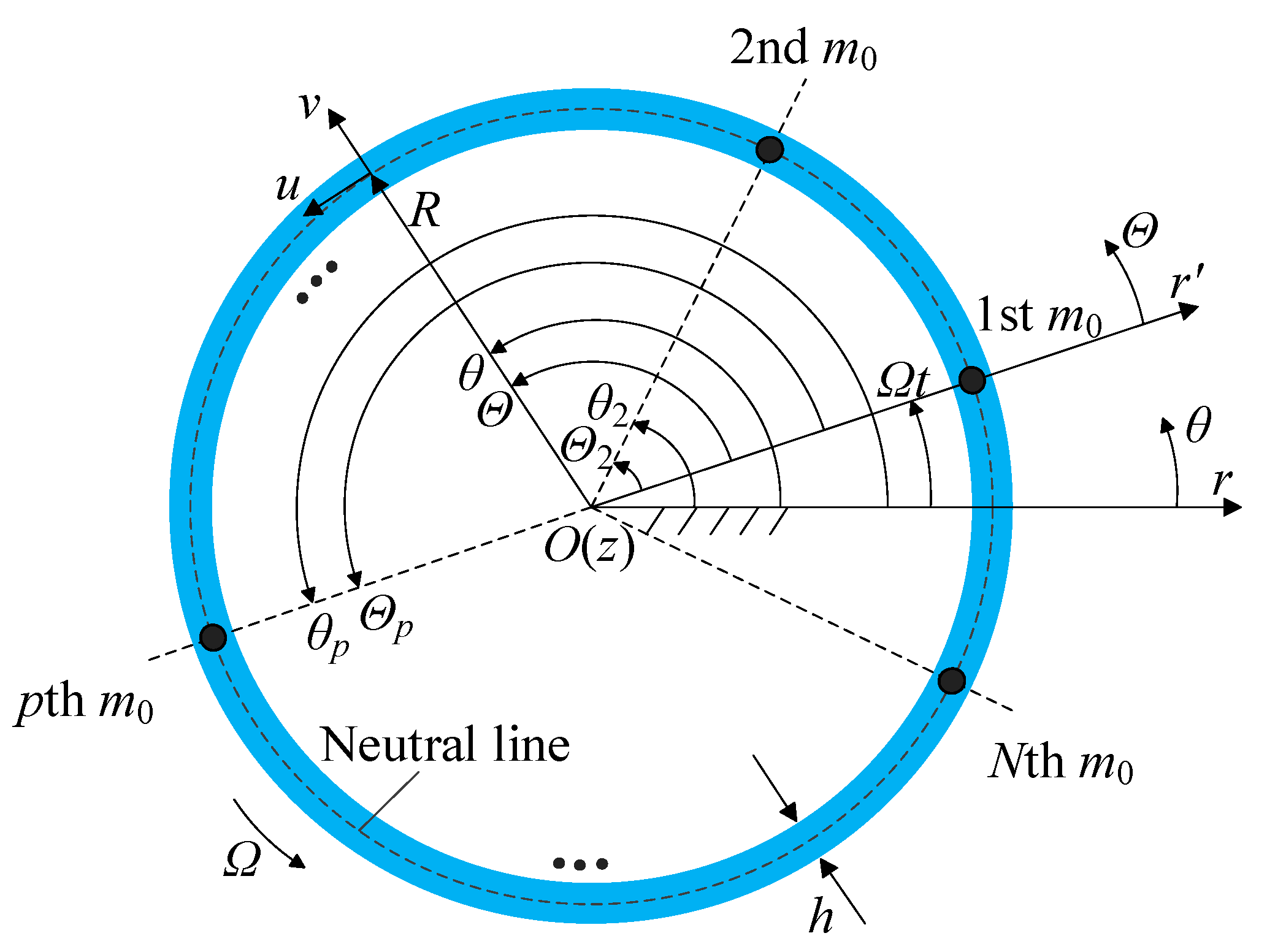
Figure 2.
The radial and tangential displacement distribution on the neutral circle for steady elastic deformation, for (a) N=2, (b) N=3, (c) N=4, and (d) N=5.
Figure 2.
The radial and tangential displacement distribution on the neutral circle for steady elastic deformation, for (a) N=2, (b) N=3, (c) N=4, and (d) N=5.
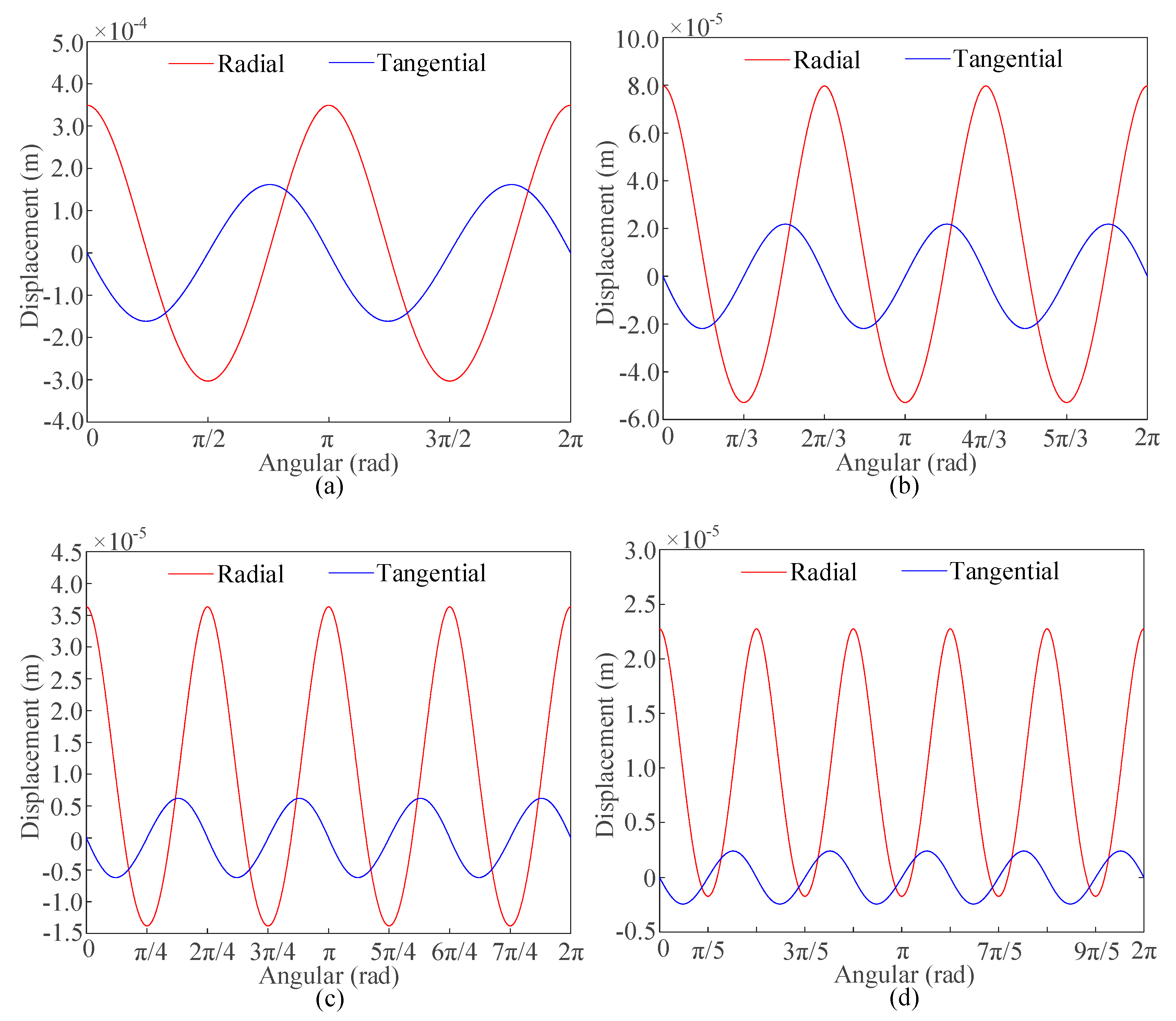
Figure 3.
Steady elastic deformation of the model with point masses, for (a) N=2 and N=3, (b) N=4 and N=5.
Figure 3.
Steady elastic deformation of the model with point masses, for (a) N=2 and N=3, (b) N=4 and N=5.
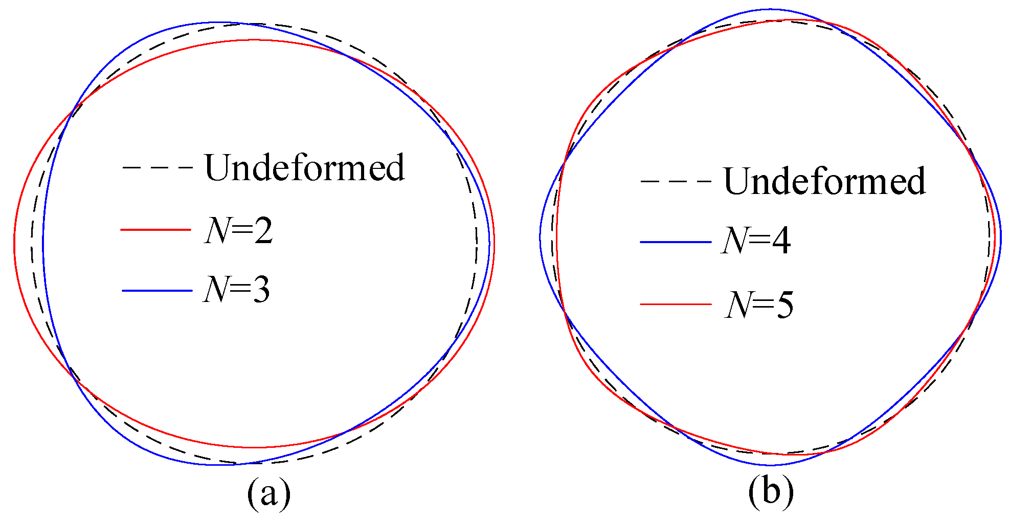
Figure 4.
Nondimensional tangential tension distribution with different number of mass imperfections when Ω=500rad/s, where the straight curves ‘---’ denote the results for perfect ring and the dashed curves ‘—’ denote the cases of (a) N=2, (b) N=3, (c) N=4, and (d) N=5.
Figure 4.
Nondimensional tangential tension distribution with different number of mass imperfections when Ω=500rad/s, where the straight curves ‘---’ denote the results for perfect ring and the dashed curves ‘—’ denote the cases of (a) N=2, (b) N=3, (c) N=4, and (d) N=5.
Figure 5.
The variation of φ(j) with rotational speed, for (a) N=2 and (b) N=3.
Figure 6.
The Coriolis effect observed in (a) ground-fixed coordinates, (b) body-fixed coordinates.
Figure 7.
Natural frequencies of traveling waves in the ring-fixed coordinates, where the dashed curves ‘---’ denote the results for perfect resonant ring, and the straight curves ‘—’ denote the cases of (a) N=2, (b) N=3, (c) N=4, and (d) N=5.
Figure 7.
Natural frequencies of traveling waves in the ring-fixed coordinates, where the dashed curves ‘---’ denote the results for perfect resonant ring, and the straight curves ‘—’ denote the cases of (a) N=2, (b) N=3, (c) N=4, and (d) N=5.
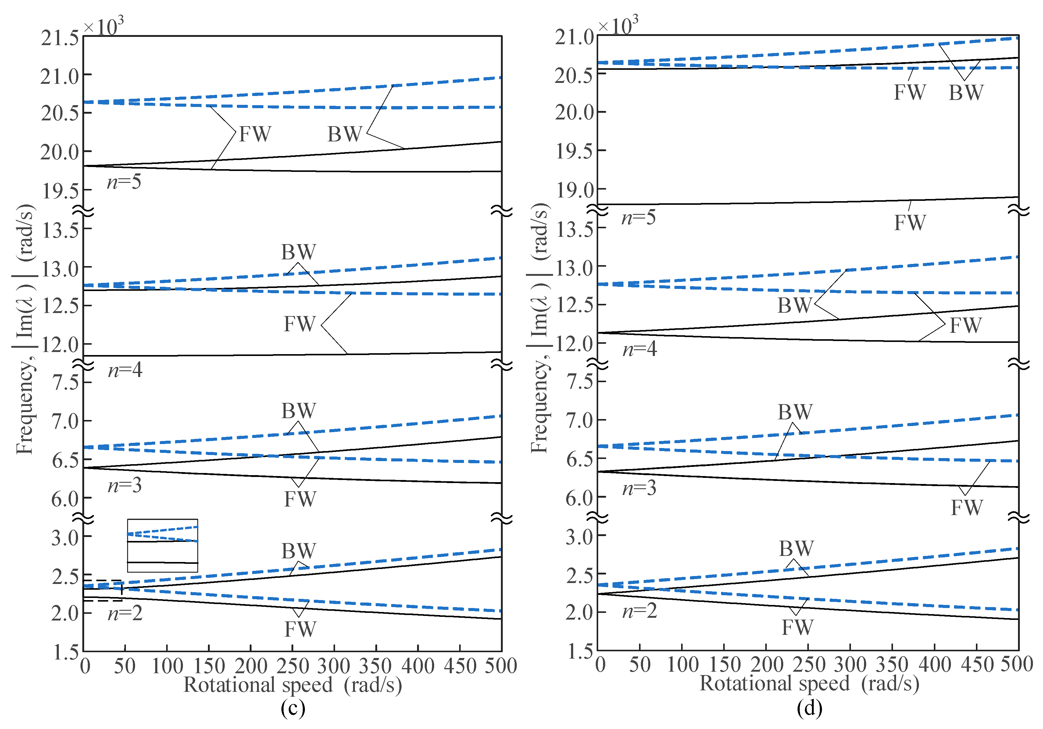
Figure 8.
The frequency difference between FW and BW of the imperfect and perfect resonant rings, for (a) N=2, (b) N=3, (c) N=4, and (d) N=5.
Figure 8.
The frequency difference between FW and BW of the imperfect and perfect resonant rings, for (a) N=2, (b) N=3, (c) N=4, and (d) N=5.
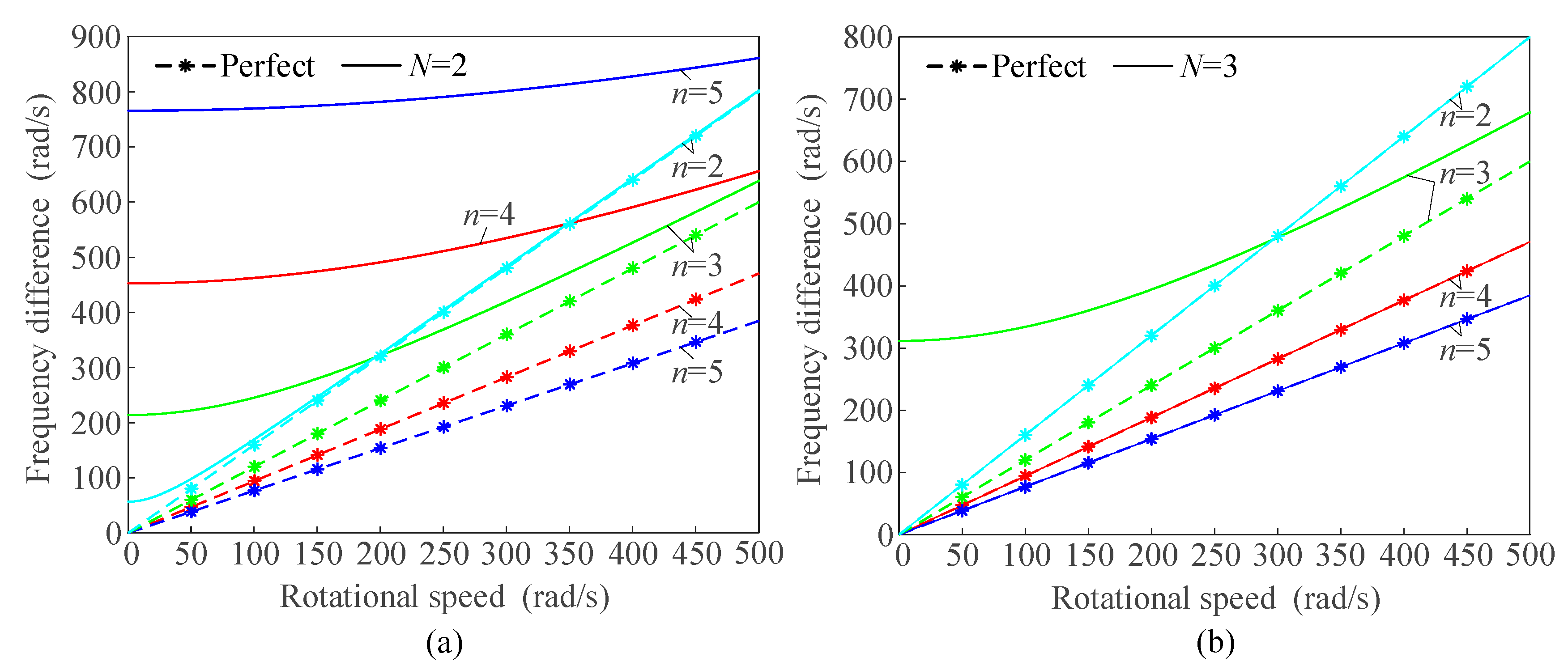

Figure 9.
Natural frequencies of traveling waves in the ground-fixed coordinates, where the dashed curves ‘---’ denote the results for perfect resonant ring, and the straight curves ‘—’ denote the cases of (a) N=2, (b) N=3, (c) N=4, and (d) N=5.
Figure 9.
Natural frequencies of traveling waves in the ground-fixed coordinates, where the dashed curves ‘---’ denote the results for perfect resonant ring, and the straight curves ‘—’ denote the cases of (a) N=2, (b) N=3, (c) N=4, and (d) N=5.
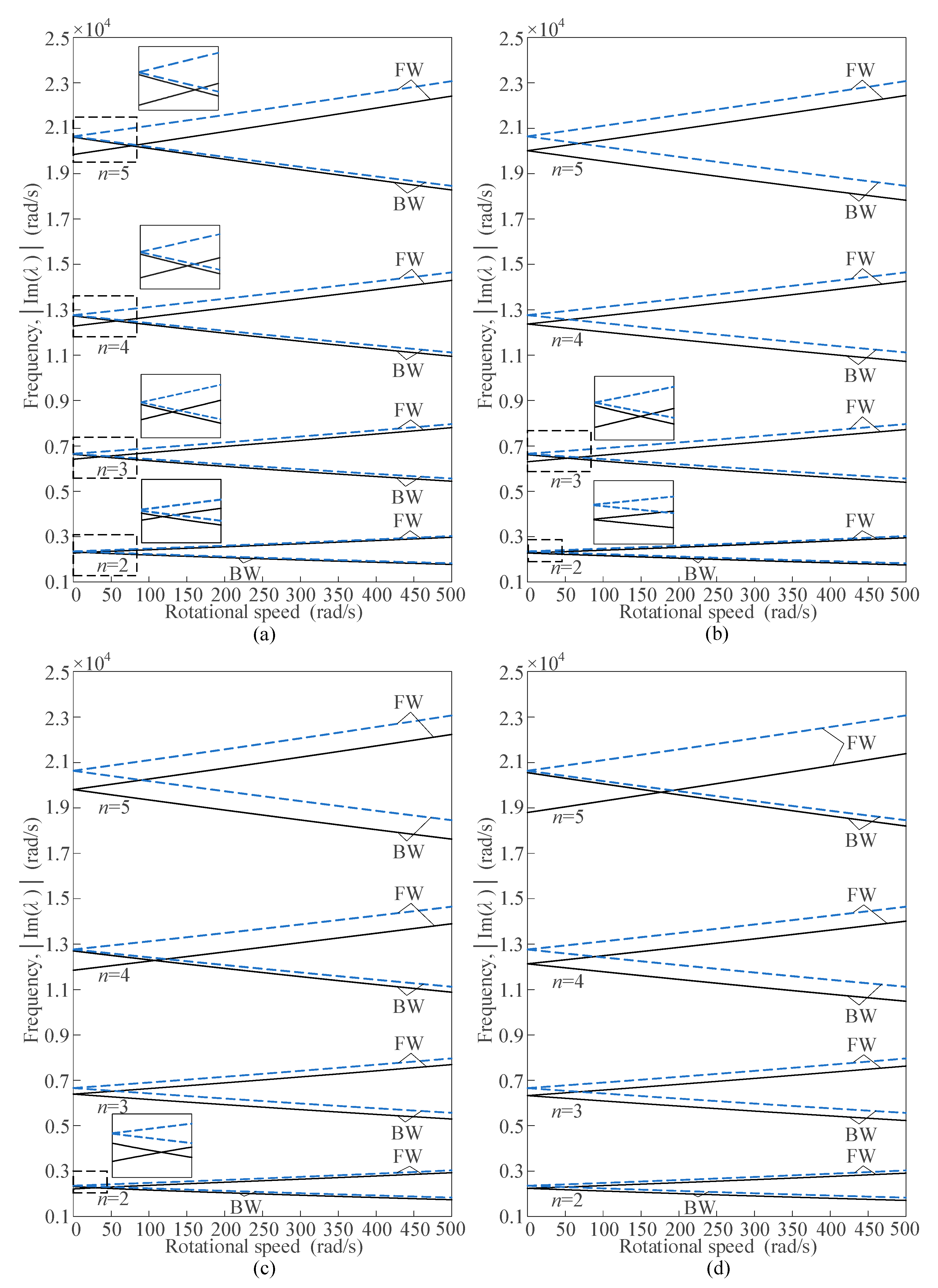
Figure 10.
The effect of the mass imperfection on rotational speeds and natural frequencies at the crosspoints.
Figure 10.
The effect of the mass imperfection on rotational speeds and natural frequencies at the crosspoints.
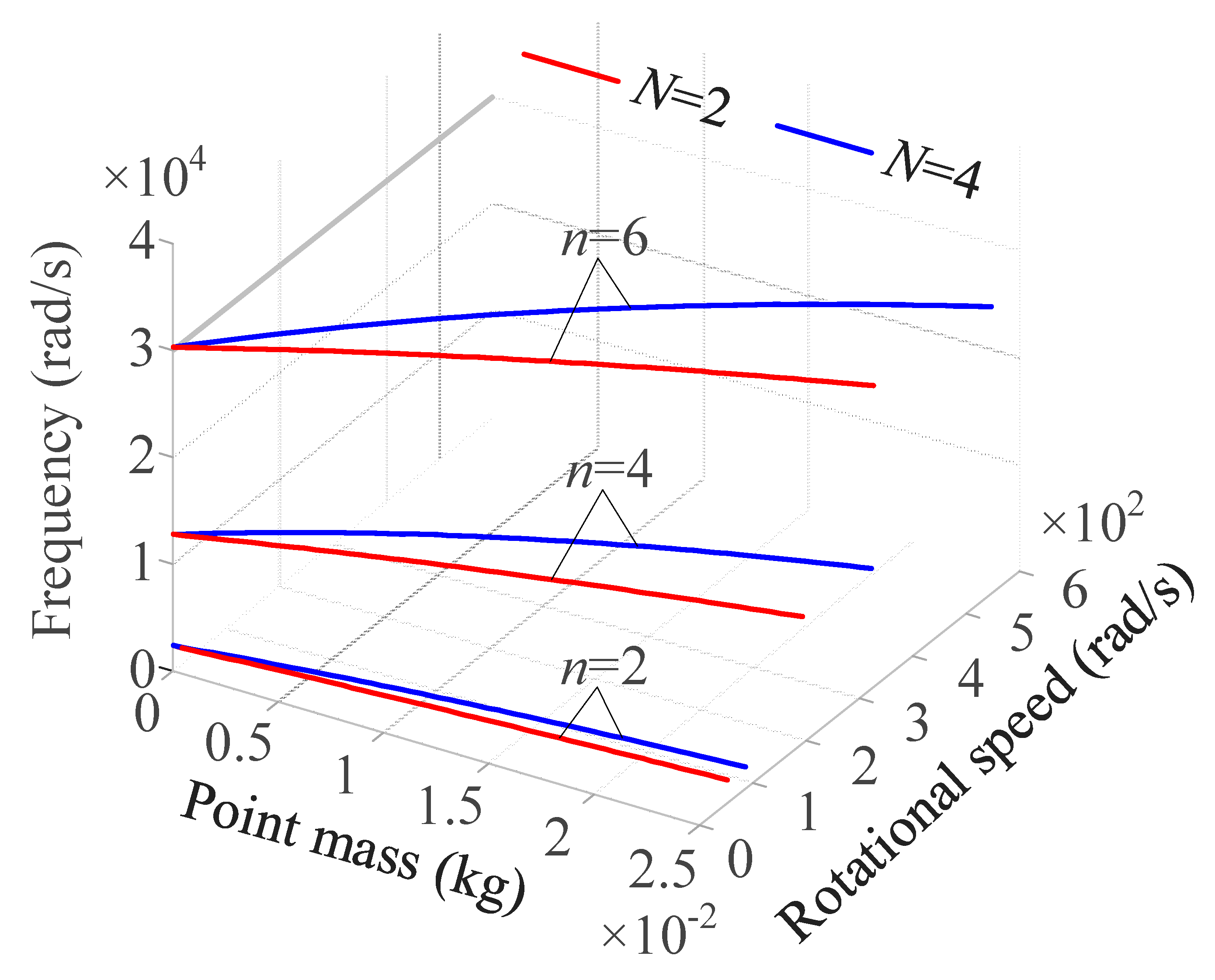

Table 1.
The parameters of the model.
| Parameters | Values and units |
| Neutral circle radius | R=0.1 m |
| Axial length | b=0.01 m |
| Young’s modulus | E =2.0×10¹¹ N/m2 |
| Density | ρ=7.8×10³ kg/m3 |
| Thickness | h=6×10⁻³ m |
| Magnitude of mass imperfection | m0=2π×10-3 kg |
| Rotational speed | Ω=500 rad/s |
Table 2.
The eigenvalues of the vibration of the system at 2n/N=int.
| Conditions | λRe | λIm | |
| 0 | |||
| 0 | |||
Table 3.
The eigenvalues of the vibration of the system at 2n/N≠int.
| Conditions | λRe | λIm | |
| 0 | |||
| 0 | |||
Table 4.
Comparisons of natural frequencies (N=4) between the finite element method and numerical calculation.
Table 4.
Comparisons of natural frequencies (N=4) between the finite element method and numerical calculation.
| Modes n | Ω (rad/s) | fFW (Hz) | fBW (Hz) | ||||
| FEM | Numerical | Diff. (%) | FEM | Numerical | Diff. (%) | ||
| 2 | 0 | 350.74 | 351.30 | 0.16 | 367.72 | 368.32 | 0.16 |
| 250 | 325.50 | 329.55 | 1.22 | 391.45 | 395.52 | 1.03 | |
| 500 | 291.56 | 306.28 | 4.81 | 421.81 | 434.91 | 3.01 | |
| 3 | 0 | 1012.70 | 1016.83 | 0.41 | 1012.70 | 1016.83 | 0.41 |
| 250 | 987.99 | 997.04 | 0.91 | 1035.80 | 1044.79 | 0.86 | |
| 500 | 966.23 | 985.33 | 1.94 | 1061.10 | 1080.82 | 1.82 | |
| 4 | 0 | 1868.30 | 1885.35 | 0.90 | 2004.70 | 2021.11 | 0.81 |
| 250 | 1865.50 | 1887.26 | 1.15 | 2006.50 | 2028.43 | 1.08 | |
| 500 | 1860.00 | 1893.47 | 1.77 | 2024.90 | 2049.76 | 1.21 | |
| 5 | 0 | 3121.80 | 3153.02 | 0.99 | 3121.80 | 3153.02 | 0.99 |
| 250 | 3104.00 | 3142.67 | 1.23 | 3135.00 | 3173.23 | 1.20 | |
| 500 | 3103.20 | 3142.04 | 1.23 | 3148.40 | 3203.31 | 1.71 | |
Diff.=(Numerical- FEM)/Numerical×100%.
Disclaimer/Publisher’s Note: The statements, opinions and data contained in all publications are solely those of the individual author(s) and contributor(s) and not of MDPI and/or the editor(s). MDPI and/or the editor(s) disclaim responsibility for any injury to people or property resulting from any ideas, methods, instructions or products referred to in the content. |
© 2025 by the authors. Licensee MDPI, Basel, Switzerland. This article is an open access article distributed under the terms and conditions of the Creative Commons Attribution (CC BY) license (http://creativecommons.org/licenses/by/4.0/).
Copyright: This open access article is published under a Creative Commons CC BY 4.0 license, which permit the free download, distribution, and reuse, provided that the author and preprint are cited in any reuse.


