Assessment Spinal Surgery Python, AI and Machine Learning Self-Assessment for Spinal Fusion Surgery Case Report

1. Background

1.1. Data Array Table

Limitations: This experimental research: sample size, data quality, no control group, selection bias.

Conflict of interest statement: Competing interests: The author declares that there are no competing interests.

Key Words:AI, Python, Machine Learning, Synthetic data, Logistic Regression, Path Analysis

1.2. Introduction:

Artificial intelligence (AI) and machine learning (ML) are part of the medical and technology landscape. This is a single case study that employs real and synthetic data generated by the AI subset, machine learning. The purpose of this presentation is to examine a method of self-assessment for spinal fusion surgery.

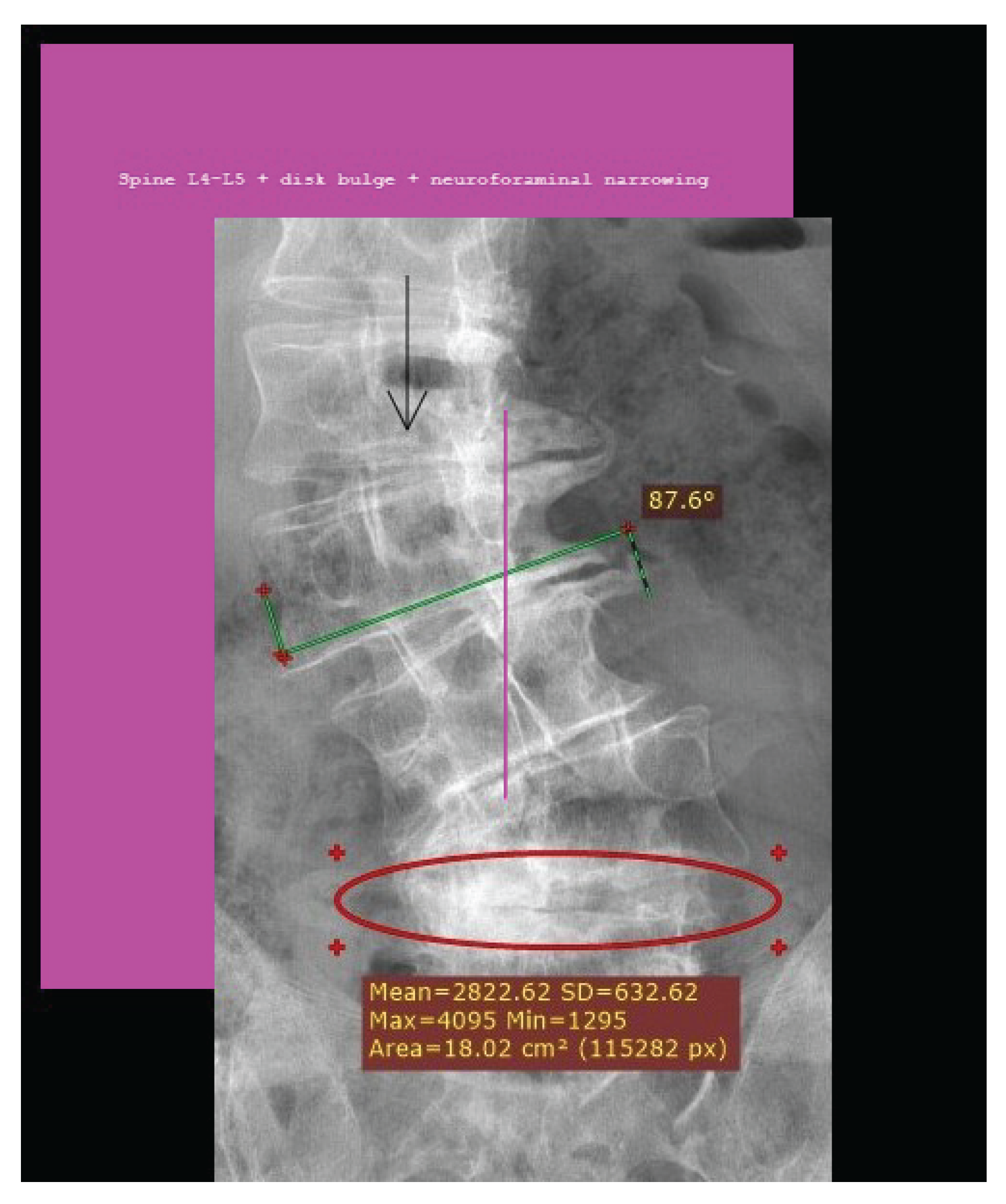
The lower back pain of a 79-year-old male runner intensified during 2021-2024. Before then, he enjoyed excellent health, improved mood, relaxation, and fitness. Muscle strain was thought to be the cause of pain. He applied ice, heat, stretched, meditated, swam, and supplemented these with over-the-counter Advil. Each had a limited impact and duration for pain reduction. He experienced tingling and numbness in his right leg, including the three right toes of his right foot. At times he felt as if he could fall.

It took 40 years of jogging experience to compress a spinal disk located in L4-L5 and crush existing spine nerves. His physician referred him for an MRI. Spinal stenosis and compressed disk were diagnosed. Complementary approaches to pain reduction were recommended. These included meditation, stretching, swimming, fast walking, yoga, Pilates, and Feldenkrais methods. The inability to attenuate pain led the patient to request an epidural. Pain decreased for 2.5 months and returned. He was informed by personal communication "Your pain is due to L4/L5 foraminal stenosis that affects the nerve roots that traverse at this level." Faced with epidurals for the remaining life span, he accepted the recommendation for surgery.

Figure 1. Spinal stenosis, L4-L5 disk bulge, neuroforaminal narrowing

Figure 1. Spinal stenosis, L4-L5 disk bulge, neuroforaminal narrowing

The literature on complementary medicine [2] advocates for approaches to pain reduction [3] but does not address the root cause of pain. After the patient underwent successful spinal fusion surgery, 2024 he applied AI skills to test whether his self-assessment questionnaire would lead to a recommendation for surgery. AI produced results comparable with those of the recommended medical protocol. The questionnaire variables were drawn from diagnostic imaging (MRI) and observed physical functioning gathered over the life course of the 79-year-old patient. The contrast in time could not be greater. A decision tree is supervised learning employing labeled data that can be entered into AI while an individual’s health is influenced over time by physical challenges, human and natural influences, and education that come to occupy consciousness. To be clear, personal choices interact with real world events, as did 40 years of jogging. The patient is the most informed expert in this regard [4] (In: Self-efficacy: the power of control). He enjoyed excellent health until lower back pain worsened over time. The pain was misattributed to muscle strain. Complementary approaches to pain control had minimal effect. Reflecting on diagnostic decisions, some are influenced by initial biases, resulting in faulty conclusions, while decisions that take time are more likely the result of better information, according to the authors of ’Fast decisions reflect biases; slow decisions do not’ led by applied mathematicians [12] at the University of Utah. This study relates to 40 years of patient experience, providers, diagnosis, and AI assessments.

Case Presentation:

Motivation for conducting this research originated in 2024 after spine fusion surgery. The skills used to generate data in this research are available to anyone willing to learn more about personal healthcare. The paper will contribute to the patient self-assessment literature. It is unique for providing patients with a model for self-selected responses. The results are not generalizable given the single case and synthetic data. However, imagine a site guiding users to construct their own questionnaire of 5 to 10 questions. Topics suitable for AI analysis include a range of applications such as mental health, addiction, physical distress, and those in combination. When numerical responses are entered, the data is entered in AI to generate results.

Figure 2. Post Spinal Lumbar Surgery

Figure 2. Post Spinal Lumbar Surgery

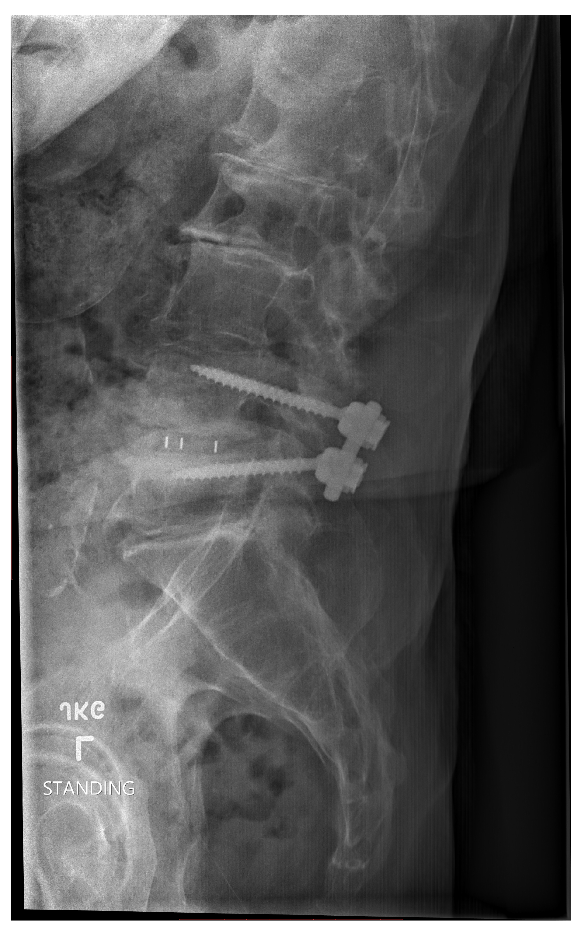
Figure 2: Post Lumbar Surgery

During spine fusion surgery, 1cc formable cellular bone (personal message surgeon) was installed at Kaiser Oakland Hospital. Subsequently, with the use of AI skills, the patient documented his path from jogging, epidurals, to surgery. Data collected from a self-assessment questionnaire was entered using Python code to create a dictionary (Table 1).

Materials and Methods

The code and results in the following sections are AI Juypter platform, [1,3,7,10,1], converted the questionnaire responses to read yes = 1, no = 0

Table 1. Research Questionnaire.

Table 1. Research Questionnaire.

Boosted Decision Tree XGBoost: o Uses Gradient Boosting to emphasize incorrectly classified samples. o Produces higher accuracy for many datasets. o Displays Feature Importance (as a bar graph) to show how influential each feature is in predicting "Surgery".

The surgery questionnaire was run through several AI platforms to check the performance and layout of the data. Stanford AI Jupyter platform was used to generate the following data and code.

The first row [1, 40, 1, 1, 1, 1, 1, 1, 1, 5, 1] corresponds to responses from the real patient. The other rows are machine learning synthetic data. Synthetic data often plays an important role in machine learning, especially when working with limited or incomplete datasets, such as in this case, where only a single data point was entered. Here is an explanation of why synthetic data is needed.

1.3. Abbreviated Data Array for Table 1

Table 1. Abbreviated Column Headings for 5x11 Data Array.

	a	b	c	d	e	f	g	h	i	j	k
Row 1	1	40	1	1	1	1	1	1	1	5	1
Row 2	0	20	1	0	0	0	0	1	0	3	0
Row 3	1	15	0	1	0	0	0	0	1	1	0
Row 4	0	5	0	1	1	1	0	0	0	5	0
Row 5	1	10	1	0	1	1	1	1	0	4	1

Table 1. Abbreviated Column Headings for 5x11 Data Array.

	a	b	c	d	e	f	g	h	i	j	k
Row 1	1	40	1	1	1	1	1	1	1	5	1
Row 2	0	20	1	0	0	0	0	1	0	3	0
Row 3	1	15	0	1	0	0	0	0	1	1	0
Row 4	0	5	0	1	1	1	0	0	0	5	0
Row 5	1	10	1	0	1	1	1	1	0	4	1

Key:

Table 2. Mean of Each Feature.

(a) Jogging	(e) X-ray	(i) Fit
(b) Time	(f) Referral	(j) Lifetime
(c) Evaluation	(g) Titanium	(k) Exercise
(d) MRI	(h) Recovery	(l) Target

Table 2. Mean of Each Feature.

(a) Jogging	(e) X-ray	(i) Fit
(b) Time	(f) Referral	(j) Lifetime
(c) Evaluation	(g) Titanium	(k) Exercise
(d) MRI	(h) Recovery	(l) Target

The mean (average) of each feature (see key) is calculated across all rows of the dataset.

For example, if the first value is 0.6, it means that, on average, the first feature identifying jogging has a value of 0.6 rows in the data.

Similarly, 18. for the second feature (Time) is the average time value over all samples. This helps you understand the central tendency of each attribute in your data set.

Proportion of ’Surgery Recommended’ (target):

The proportion is essentially the average of the target values, the fraction of where surgery is recommended.

A proportion of 0.4 means that 40 percent of the examples in the dataset have the target value 1 (indicating that surgery is recommended). These metrics provide a basic overview of the dataset, helping to highlight patterns or imbalances in the data. For example, if most target values are 0, it suggests an imbalance that could affect a machine learning model if not addressed.

Results Table

Mean of each characteristic: [0.6 18 0.6 0.6 0.6 0.6 0.4 0.6 0.4 3.6] Mean of Jogging: 0.60 Mean of Time: 18.00 Mean of Evaluation: 0.60 Mean of MRI: 0.60 Mean of X-ray: 0.60 Mean of Referral: 0.60 Mean of Titanium: 0.40 Mean of Recovery: 0.60 Mean of Fit: 0.40 Mean of Lifetime Exercise: 3.60

Mean of the target, surgery: 0.40

Proportion of ’Surgery Recommended’: 0.4

Mean Values Table 1

Table 3. Mean Values of Each Feature with Smaller Font.

Mean	a	b	c	d	e	f	g	h	i	j	k
Value	0.6	18.0	0.6	0.6	0.6	0.6	0.4	0.6	0.4	3.6	0.04

Table 3. Mean Values of Each Feature with Smaller Font.

Mean	a	b	c	d	e	f	g	h	i	j	k
Value	0.6	18.0	0.6	0.6	0.6	0.6	0.4	0.6	0.4	3.6	0.04

Explanation of Means:

• Mean a: Jogging, Mean = 0.60
• Mean b: Time, Mean = 18.00
• Mean c: Evaluation, Mean = 0.60
• Mean d: MRI, Mean = 0.60
• Mean e: X-ray, Mean = 0.60
• Mean f: Referral, Mean = 0.60
• Mean g: Titanium, Mean = 0.40
• Mean h: Recovery, Mean = 0.60
• Mean i: Fit, Mean = 0.40
• Mean j: Lifetime Exercise, Mean = 3.60
• Mean k: Target, Mean = 0.04

Each column in the array corresponds to a numerical representation of a feature of the questionnaire. Here is an example breakdown:

1. Columns (Features): These represent the key questions in the questionnaire, transformed into numerical values. o Jogging: Binary (1 for "Yes," 0 for "No") o Time: Numeric (e.g., 40 years = 40) o Evaluation, MRI, X-ray: Binary (1 for "Yes," 0 for "No") o Referral, Surgery, Consultation: Binary (1 for "Yes," 0 for "No") o Life-time exercise: A custom scale (e.g., 5 for "five days per week", proportionally reduced for fewer days)

Other fields might be omitted if they represent free-text inputs (like "Cause" or "Diagnosis") since these require processing techniques like unsupervised learning or natural language processing (NLP). Alternatively, these might be encoded as categories.

2. Rows (Patient Cases): Each row in the data is a synthetic patient case representing a possible combination of answers. For example: o Row [1, 40, 1, 1, 1, 1, 1, 1, 1, 5, 1] might represent:

* Jogging contributed to pain. * Patient jogged for 40 years. * Evaluations such as magnetic resonance imaging and X-rays were completed. * Referrals, consultations, and recommendations for surgery were favorable. * Patient exercised 5 days a week.

Why is synthetic data useful in this case? 1. Simulating Real-World Scenarios: Generating synthetic patient cases allows the model to understand the potential variability in real-world data. Different years of jogging, varying levels of fitness, or cases where certain evaluations were not performed all contribute to a realistic training dataset. 2. Performance of the test model: With multiple samples, model performance can be tested on various combinations of inputs. For example, how would the model handle cases where no MRI was performed but surgery was still recommended? 3. Generalization: With only a single questionnaire, a model would "memorize" that one case instead of learning general patterns. Synthetic data helps mitigate this issue, making the model generalize better to unseen data. 4. Protection of privacy: In this study, real patient data was available (e.g., no access to datasets and privacy reasons), synthetic data allows the development of models and workflows without compromising personal health information (PHI) if real patients were included. Summary: the synthetic data set was generated to prepare the data set for machine learning or statistical analysis, where a numerical format and sufficient diversity of samples are essential. This ensures that the model can be trained, tested, and perhaps applied to broader real-world cases, even when only a single example (as in this questionnaire) is initially available. Synthetic data was generated around the data of this single patient using the mean values calculated for each characteristic. The question of how this works and how synthetic data might have been generated from these single real patient’s data is examined.

Understanding the Mean Values

The mean of each characteristic was provided as: [ 0.6, 18, 0.6, 0.6, 0.6, 0.6, 0.4, 0.6, 0.4, 3.6 ]

Each value represents the average of a particular feature (column) in the data set. If you had only one real patient (the first row), the remaining synthetic data must have been generated around this reference mean to simulate multiple records.

Here is what likely happened: 1. First Row as Real Data: The first row in the data array represents the author’s data. From there, the mean calculation for each feature is a direct reflection of the first row combined with the synthetic data. 2. Role of Synthetic Data: To fill the dataset, synthetic data introduced variability based on the real patient’s data (mean values). These synthetic rows simulate hypothetical patients with differing but similar attributes, allowing the data set to be expanded for analysis or machine learning training. 3. How were the synthetic rows generated? The synthetic rows were likely generated using techniques such as: Random sampling around mean values: synthetic data could be created by using a probability distribution (for example, normal distribution) with mean values from the real patient and introducing some spread (variance). For example:

* Continuous features (for example, "Time" = 40 years) could vary by ±some random factor. * Binary features (for example, "MRI" = 1) could randomly flip between 0 and 1 with the mean as the probability (for example, 0.6 means 60.)

Slight random noise might have been added to continuous data based on the real row to create diversity. Noise is a pattern that follows a normal distribution curve.

Why Use Synthetic Data from a Single Feature?

Synthetic data generated to enrich the dataset while ensuring that the AI system has enough variation to learn general patterns. There are several reasons for doing this: 1. Limitations of a single record: Having only one real patient isn’t sufficient to train a machine learning model. A single record does not contain enough diversity for the model to generalize the predictions to other patients. 2. Mean as Central Tendency: The mean values act as a useful representation of the typical or average attributes of a patient. New synthetic patients can be generated around these values to simulate a realistic dataset. 3. Small data set simulation: If only synthetic data from a single record are available, generating new synthetic records expands the dataset, helping the model learn meaningful patterns while avoiding overfitting to one specific input. 4. Flexibility for Machine Learning: Machine learning algorithms typically perform better when trained on datasets with diverse examples. Generating synthetic data introduces variation in otherwise limited datasets, improving the robustness of the model.

Importance of Variability in Synthetic Data Purely duplicating the single real patient row would not improve the model because it would "memorize" that single example rather than learn useful generalizations. By generating variability that still reflects the original data, the synthetic samples better approximate the population while being distinct enough to improve training.

Final Remarks

Synthetic data in this case have likely been generated around the single patient’s feature mean, introducing variability to fill out a usable dataset. This is a practical and often necessary approach when working with limited real-world data but needing to build robust models.

How to run the program:

1. Install Required Libraries: run pip install pandas scikit-learn xgboost matplotlib 2. Run the following code: Submit to Python IDE or Jupyter, notebook, and then execute. 3. Saved output:

Adjustments

What is Boosting?

Boosting is a powerful machine learning technique that is used to improve the accuracy and performance of weak models (classifiers or regressors) by combining them into a stronger model. It is an ensemble learning method. This method combines several models rather than relying on a single one. Boosting works iteratively by training multiple weak learners (e.g., decision trees with limited depth as in this study) in sequence, and each subsequent model focuses on the mistakes made by the previous ones. See Figure 1.

1.4. Key Characteristics of Boosting

1. Weak learner: Each individual model (or "weak learner") performs slightly better than random guessing (e.g., small decision trees). 2. Sequential Learning: The models are trained in sequence, trying to correct the errors of the previous models. 3. Weighted votes: In the end, the models are combined in a weighted manner to make the final prediction, giving more weight to models with lower error rates.

A popular example of boosting algorithms is AdaBoost (Adaptive Boosting), which adjusts the weights of training instances and models based on their performance. Other advanced boosting algorithms include gradient boost, XGBoost, and LightGBM.

Purpose of Boosting

The primary purpose of boosting is to: 1. Improve accuracy: Boosting increases the accuracy of predictions by addressing the shortcomings of weak learners. By iteratively focusing on difficult cases (e.g., misclassified data points), it creates a more robust model. 2. Reduce bias: the bias of a single weak learner by iteratively improving their performance through training. 3. Handle Complex Data: Boosting methods can handle non-linear relationships and complex data because they combine multiple models, each focusing on specific parts of the data.

Accuracy of Boosting

Boosting models are known for their high accuracy and performance, making them widely used in machine learning tasks, including: * Classification * Regression * Ranking (e.g., recommendation systems) Their accuracy typically depends on the following factors: 1. Quality of data: Boosting is sensitive to noisy data and outliers because it tries to fit the data very closely. If the data contains errors or noise, boosting can overfit. 2. Base Models: The performance of boosting depends on the choice of weak learners. For example, decision stumps or shallow trees are commonly used for their simplicity. 3. Hyperparameter Tuning: Boosting algorithms have many hyperparameters (like learning rate, number of estimators, etc.), and choosing the right combination is crucial to achieving high accuracy. 4. Overfitting Risk: If not carefully tuned, boost models can overfit to the training data, lowering their performance on unseen data.

Advantages of Boosting

* Achieves state-of-the-art performance in many machine learning tasks. * Reduces bias and variance for better generalization. * Can work well with less preprocessing of data compared to other techniques. Disadvantages of Boosting * Sensitive to outliers and noise in the data, which can degrade performance. * Training can be computationally expensive for large datasets. * Hyperparameter tuning often requires significant effort for optimal performance. In summary, boosting significantly improves the accuracy of weak learners, making it one of the most effective techniques in machine learning. However, its performance relies on having clean data and appropriate hyperparameter tuning to avoid overfitting.

2. Supplementary Material

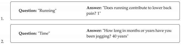
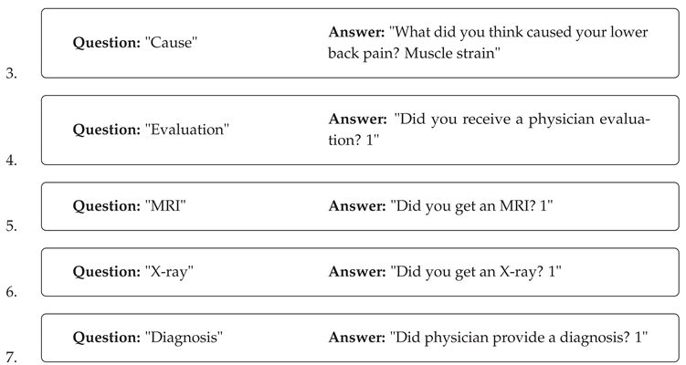
Section 1$Thefollowingstructurerepresentsthequestionsaskedinthemedicalquestionnaire.$ This data set could potentially inform the synthetic dataset by modeling responses to these questions.

questionnaire = ["Jogging": "Does jogging contribute to lower back pain? 1", "Time": "How long in months or years have you been jogging? 40 years? 1", "Cause": "What did you think caused your lower back pain? Muscle strain 1", "Evaluation": "Did you receive a physician evaluation? 1", "MRI": "Did you get an MRI? 1", "X-ray": "Did you get an X-ray? 1", "Diagnosis": "Did you get a diagnosis? 1", "What was your diagnosis": "stenosis of lumbar intervertebral foramina 1", "referral": "Were you referred to physical medicine for an epidural? 1", "Epidural": "Did you get an epidural? 1", "Surgery": "Were you referred to physical medicine for L4L5 minimally invasive surgery? 1", "Consultation": "Was the surgeon consultation: kind, competent, expert? 1", "Disk": "Did the consultation include a new plastic carbon fiber disk recommendation? 1", "Titanium": "Did the recommendation include one titanium rod with two screws? 1", "Risks": "Were you advised of the risks of surgery? 1", "Recovery": "Did the surgeon discuss recovery from surgery with you? 1", "Fit": "Is the patient physically and mentally fit? 1", "What is your week: running, swimming, weight fitness? 1", "Do you feel fit and healthy after 5 months post-surgery?": "1", ]

Table 4. Synthetic Dataset - Question & Response

Question	Response
Surgery (1 = yes, 0 = no)	1, 0, 1, 0, 0, 1, 1, 0, 0, 1
Titanium rod usage (1 = yes, 0 = no)	1, 0, 1, 0, 0, 1, 0, 0, 0, 1
MRI taken (1 = yes, 0 = no)	1, 0, 1, 0, 0, 1, 1, 1, 0, 1
Consultation quality (1 = good, 0 = poor)	1, 1, 0, 0, 1, 1, 1, 0, 0, 1
Recovery status (1 = good, 0 = poor)	0, 1, 1, 0, 0, 1, 1, 0, 0, 1
Patient’s fitness	1, 1, 1, 0, 1, 1, 1, 0, 0, 1
Outcome (1 = positive, 0 = negative)	1, 0, 1, 0, 0, 1, 1, 0, 0, 1

Table 4. Synthetic Dataset - Question & Response

Question	Response
Surgery (1 = yes, 0 = no)	1, 0, 1, 0, 0, 1, 1, 0, 0, 1
Titanium rod usage (1 = yes, 0 = no)	1, 0, 1, 0, 0, 1, 0, 0, 0, 1
MRI taken (1 = yes, 0 = no)	1, 0, 1, 0, 0, 1, 1, 1, 0, 1
Consultation quality (1 = good, 0 = poor)	1, 1, 0, 0, 1, 1, 1, 0, 0, 1
Recovery status (1 = good, 0 = poor)	0, 1, 1, 0, 0, 1, 1, 0, 0, 1
Patient’s fitness	1, 1, 1, 0, 1, 1, 1, 0, 0, 1
Outcome (1 = positive, 0 = negative)	1, 0, 1, 0, 0, 1, 1, 0, 0, 1

Figure 4 Decision Tree Visualization

Figure 3. Decision Tree Spine Fusion Surgery

Figure 3. Decision Tree Spine Fusion Surgery

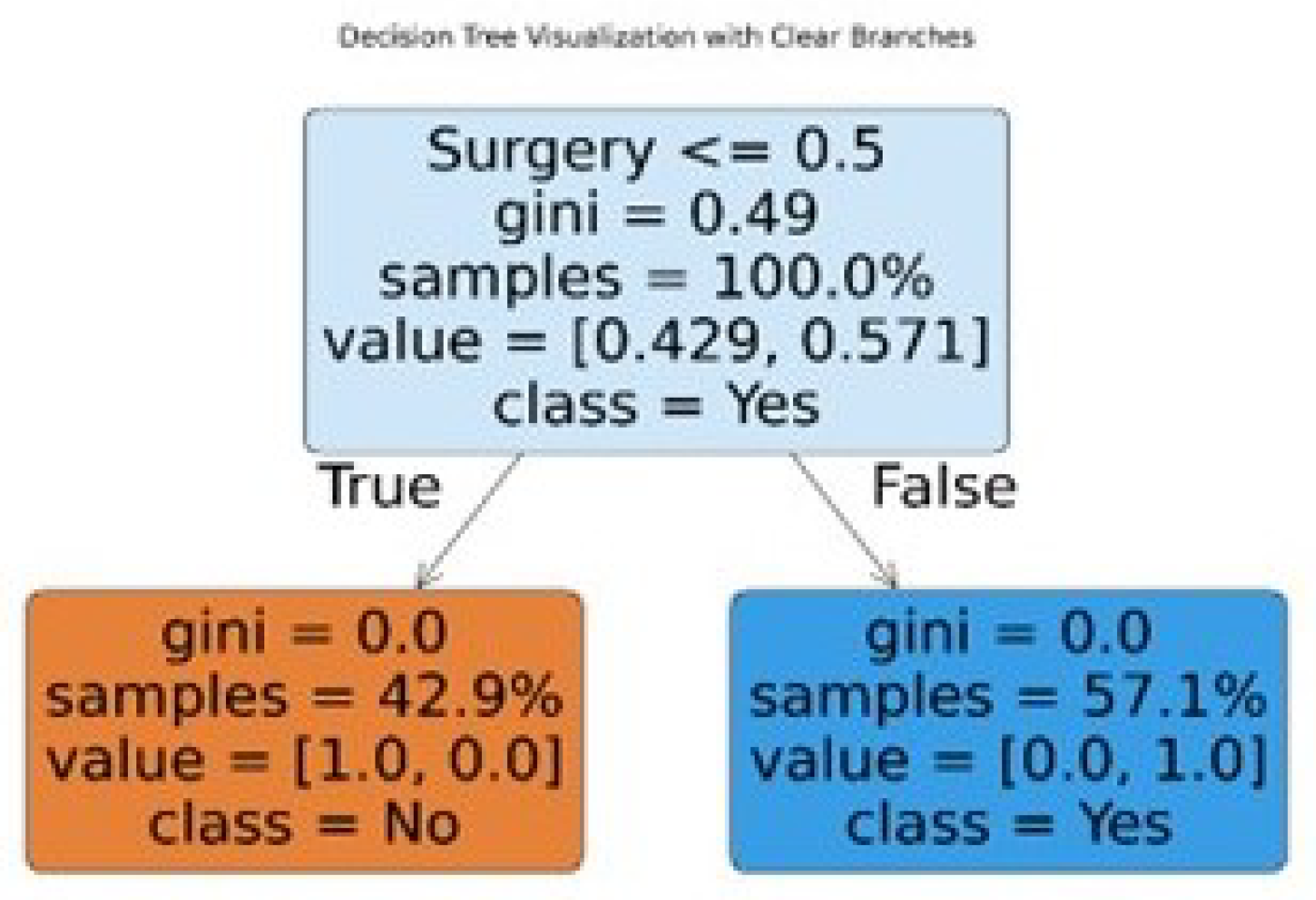
Decision Tree accuracy: 1.0 Gradient Boosting accuracy: 1.0 Decision Tree Cross-Validation Scores: [0. 1. 1. 1. 1.] Decision Tree Cross-Validation Mean accuracy: 0.8 Gradient Boosting Cross-Validation Scores: [1. 1. 1. 1. 1.] Gradient Boosting Cross-Validation Mean Accuracy: 1.0

booktabs

Table 5. Combined Classification Report and Regression/Model Fitting Results

Classification Report					Regression/Model Fitting Results
	Precision	Recall	F1-Score	Support	lval	op	rval	Estimate
0	1.00	1.00	1.00	2
1	1.00	1.00	1.00	1
Accuracy			1.00	3
Macro Avg	1.00	1.00	1.00	3
Weighted Avg	1.00	1.00	1.00	3
					Std. Err	z-value	p-value

Table 5. Combined Classification Report and Regression/Model Fitting Results

Classification Report					Regression/Model Fitting Results
	Precision	Recall	F1-Score	Support	lval	op	rval	Estimate
0	1.00	1.00	1.00	2
1	1.00	1.00	1.00	1
Accuracy			1.00	3
Macro Avg	1.00	1.00	1.00	3
Weighted Avg	1.00	1.00	1.00	3
					Std. Err	z-value	p-value

Logistic regression predicts categorical binary outcomes using a linear equation. The reported accuracy is 1.0, or 100

Classification Report

The classification report breaks down the model’s performance metrics by class (e.g., 0 and 1 in your example). For class 0: * Precision: 1.00 ? All instances predicted as class 0 were correct. * Recall: 1.00 ? All class 0 instances in the dataset were correctly identified. * F1 score: 1.00 ? F1 is the harmonic mean of precision and recall, so both being perfect results in an F1 score of 1.00. * Support: 2 indicates that there are 2 instances of class 0 in the test set. For Class 1: * Precision, Recall, F1-score: All are 1.00 ? This indicates perfect predictions for class 1 as well. * Support: 1 indicates that there is only one instance of class 1 in the test set. Overall Metrics: * Accuracy: 1.00 ? 100* Macro Average: 1.00 ? Average of precision, recall, and F1-score across all classes (unweighted). * Weighted average: 1.00 is similar to macro, but weighted by the number of samples in each class.

* The bar chart represents the coefficients of the logistic regression model, which are the weights assigned to the input features (X.columns). * Magnitude of coefficients: o High positive coefficient: The feature contributes strongly to predicting the positive class (for example, surgery in this self-assessment questionnaire by the Lamson case example). o High negative coefficient: The characteristic negatively correlates with the prediction. o Near-zero coefficients: The feature has minimal impact on the predictions. * In this dataset, surgery appears to contribute positively to predicting the outcome, while some associations appear negative.

Regression Statistics Table The regression table reflects the relationships between predictors (surgery, MRI) and outcomes. Here is a breakdown of the key rows in these data:

Key Metrics: * Estimate: The coefficient for each variable in the regression that represents its effect on the outcome. o Example: Outcome Surgery ? Estimate = 0.970426 This means that surgery is positively associated with the predicted outcome. * Std. Err (Standard Error): Measure of the variability of the estimate (a lower value indicates that the estimate is more reliable). * p-value: Indicates the significance of the coefficient: o A p-value < 0.05 suggests the feature significantly affects the outcome (e.g., Outcome Surgery with a p-value of 0.0000). o Features like Outcome MRI have a high p-value (0.752262), which means that they lack statistical significance.

Interpretation of rows: 1. Outcome Surgery: positive coefficient (0.970426) and significant effect (p-value = 0.000000), indicate that surgery strongly predicts the outcome. 2. Outcome MRI: Very low estimate (0.024584) and nonsignificant (p-value = 0.752262). This suggests that MRI has little predictive power for the outcome. 3. Recovery MRI: Negative estimate (-0.240345) and nonsignificant (p-value = 0.584153), showing a strong predictor of recovery. 4. Recovery Surgery: Positive association (estimate = 0.790293) but with borderline significance (p-value = 0.066236). Surgery might influence recovery, but more data is needed to confirm this. Correlations: * Outcome Outcome (0.004901): Models autocorrelation; significant with p-value = 0.025347. * Recovery Recovery (0.155798): Reveals a relationship within recovery predictions.

Summary of Findings

* High Model Accuracy: The accuracy of 1.0 indicates perfect predictions, but the tiny dataset suggests that these results need further validation on larger data to eliminate overfit concerns. * Importance of features: o Surgery has a positive effect on results and recovery. o MRI has minimal impact. * Statistical Insight: Surgery is statistically significant for modeling, but may not be a key predictor.

Figure 3Logistic Regression Visualization

Purpose: Logistic and multiple regression defined; * Logistic regression: Logistic regression is used when the dependent variable (outcome) is categorical, often binary (e.g., 0 or 1, True or False, Yes or No). Predicts the probability of an event occurring (e.g., the chance that a patient has a disease based on certain predictors). In this case, it is surgery. See Figure 3, column 1 importance of the features.

* Multiple regression: Multiple regression is used when the dependent variable (outcome) is continuous such as height, weight, income. The value of the dependent variable is based on one or more independent variables.

2.1. Results and Discussion

AI, Statistical Logistic Regression and Path Analysis demonstrate associations of patient questionnaire with outcome, surgery. It has been enlightening to pursue cause and effect of lower back pain through personal history, assessment, diagnosis, treatment, to spinal fusion surgery. The healthcare provided to this patient has been quality-of-life extending and invaluable. AI has the potential to integrate patients in therapeutic decision-making with data quality, model boosting, and collaboration for the purpose of improving diagnosis and treatment recommendations. Reference [2] was consulted regarding lower back risk factors. Patient satisfaction with spine fusion surgery explored in item [14]. Reflected upon whether physicians, hospitals, and patients could benefit from individualized self-assessment questionnaires when considering spinal fusion surgery [9], and the significant potential for developing preoperative pain intensity wearable sensors to facilitate diagnosis and recommendation for spine fusion surgery [13]. How Pain from L4-L5 is Transmitted Sergiu Pasca, a neuroscientist at Stanford University, co-authored a study that reports creation of neural assembloids in 2017 [19] [5]. Pasca and his team have recently generated a four-component sensory circuit. The team developed four neuronal clusters in sequence sensory, spinal, thalamic, and cortical and left them to grow and find their own connections[17]. The significance of this research is the establishment of a pathway that may mirror transmission of pain from spine to brain. Dr. Eric Chang (Associate Professor, Zucker School of Medicine at Hofstra/Northwell, Molecular Medicine) provided (personal contact) information about pain. In the L4-L5 region of the spine, pain is transmitted by dorsal root ganglia (DRG) neurons that are part of the somatosensory system. It is possible to record from DRGs as this is frequently done in animal models, but there are also some studies in humans [11]. Mello, D. and A.H. Dickenson describe L4-L5 spinal cord transmission of pain [7]. Image and dermatome description of pain transmission from spine to brain [20]. Development of a wearable sensor may capture this activity and possess meaningful data that contribute to medical decision making. Reference [8] was included to document the increasing and varied use of AI in medicine. FDA press release on 5-9-25. The content endorses use of AI. "I was blown away by the success of our first AI-assisted scientific review pilot. We need to value our scientists time and reduce the amount of non-productive busywork that has historically consumed much of the review process. The agency-wide deployment of these capabilities holds tremendous promise in accelerating the review time for new therapies" Dr. Makary. The generative AI tools allow FDA scientists and subject-matter experts to spend less time on tedious, repetitive tasks that often slow down the review process. This is a game-changer technology that has enabled me to perform scientific review tasks in minutes that used to take three days, said Jinzhong (Jin) Liu, Deputy Director, Office of Drug Evaluation Sciences, Office of New Drugs in FDAs Center for Drug Evaluation and Research (CDER). Numbers: Projections of Single-level and Multilevel Spinal Instrumentation Procedure Volume (450,000) and Associated Costs for Medicare Patients to 2050 [15]. In a report published in 2021, spinal fusion accounted for the highest aggregate hospital costs (14.1 billion across 455,500 procedures in 2018) of any surgical procedure performed in US hospitals.[16].

The author is grateful for the recommendations and expertise provided during the preparation of this work.

References

- 2024. ai with python.
- 2024. harvard professional certificate in data science: machine learning with ai and python, https://online-learning.harvard.edu/.
- 2024. stanford code-in-place.
- bandura, a. 1997. self efficacy the exercise of control.
- birey, f. , andersen j., makinson cd, islam s., wei w., huber n., fan hc, metzler krc, panagiotakos g., thom n., orourke na, steinmetz lm, bernstein ja, hallmayer j., and huguenard. 2017. assembly of functionally integrated human forebrain spheroids.
- Kuo Calvin, Royse Kathryn E., Prentice Heather A., Harris, Jessica E., Guppy, and Kern H. 2022. Are Octogenarians at Higher Risk of Complications After Elective Lumbar Spinal Fusion Surgery: Analysis of a Cohort of 7880 Patients from the Kaiser Permanente Spine Registry. Spine.
- d’mello, r. and dickenson a.h. 2008. spinal cord mechanisms of pain.
- elemento olivier, khozin sean, and sternberg cora. 2025. the use of artificial intelligence for cancer therapeutic decision making.
- hamdan, t.a. and abdulsalam s.j. 2020. patient satisfaction in spine practice.
- jetbrains and pycharm. 2025. the python ide for professional developers.
- kashkoush ai, gaunt ra, fisher le, and [other authors]. 2019. recording single and multi unit neuronal action potentials from the surface of the dorsal root ganglion.
- linn samantha, lawley sean, karamched bhargav, kilpatrick zachary, and josi. 2024. fast decisions reflect biases slow decisions do not.
- K. M. Little, J. S. Taylor, and M. Schlosser. 2016. Reducing Unwarranted Variation in Care to Improve Health Outcomes. Healthcare Financial Management 2016, 70, 88. [Google Scholar]
- Stevens Joel, M. , Delitto Anthony, Khoja Salim S., [Other Author 1], and [Other Author 2]. 2021. Risk Factors Associated With Transition From Acute to Chronic Low Back Pain in US Patients Seeking Primary Care. JAMA Network Open 2021, 4. [Google Scholar]
- mani, k. , kleinbart e., goldman s.n., golding r., gelfand y., murthy s., eleswarapu a., yassari r., fourman m.s., and krystal j. 2024. projections of single-level and multilevel spinal instrumentation procedure volume and associated costs for medicare patients to 2050. [CrossRef]
- mcDermott, k.w. and liang l. 2018,2021. overview of operating room procedures during inpatient stays in u.s. hospitals.
- miura, y. , kim j.i., jurju o., kelley k.w., yang x., chen x., thete m.v., revah o., cui b., and pachitariu m. 2024. Assembloid model to study loop circuits of the human nervous system. (2024). Preprint on bioRxiv. Available from. [CrossRef]
- musk. 2025. grok.
- Pasca and Sergiu. 2025. Assembloids.
- whitman, p.a. launico m.v., and adigun o.o. 2025. anatomy, skin, dermatomes.
Disclaimer/Publisher’s Note: The statements, opinions and data contained in all publications are solely those of the individual author(s) and contributor(s) and not of MDPI and/or the editor(s). MDPI and/or the editor(s) disclaim responsibility for any injury to people or property resulting from any ideas, methods, instructions or products referred to in the content. |
© 2025 by the authors. Licensee MDPI, Basel, Switzerland. This article is an open access article distributed under the terms and conditions of the Creative Commons Attribution (CC BY) license (http://creativecommons.org/licenses/by/4.0/).
Copyright: This open access article is published under a Creative Commons CC BY 4.0 license, which permit the free download, distribution, and reuse, provided that the author and preprint are cited in any reuse.