Submitted:
04 July 2025
Posted:
08 July 2025
You are already at the latest version
Abstract
A study was conducted at CONCRENORTE SAS to optimize mix designs by reducing cement in concrete production with a reliability of 85%. To achieve this goal, tests were performed to determine aggregate parameters using the ACI-211 method, and then designs for A/C ratios ranging from 0.35 to 0.75 were developed. The RNL method was used for the use of the combined sand. To verify the curve obtained, a mix design was performed that showed that the expected reliability of 85% was achieved. The mix design was used with 50% limestone sand and 50% Sinu river sand, all in compliance with Colombian technical standard procedures. The aim was to use available materials to adjust the water/cement ratio curve for 28-day strength.
Keywords:
Optimization
; mix design
; A/C ratio
; reliability
; RNL
; strength
Laboratory Results
River Sand (Lorica)
For each test performed, the mean and standard deviations were found to be used as representative data:

Table 1.
Average river granulometry result.
| Sieve | Opening (mm) | Average | Standard deviation |
| 3/8" | 9.5 | 99.98 | 0.079 |
| No. 4 | 4.75 | 99.61 | 0.392 |
| No. 8 | 2.36 | 98.88 | 0.916 |
| No. 16 | 1.18 | 96.71 | 2,395 |
| No. 30 | 0.6 | 92.26 | 5,313 |
| No. 50 | 0.3 | 29.42 | 11,637 |
| No. 100 |
0.15 | 2.49 | 1,612 |
| No. 200 |
0.075 | 0.43 | 0.277 |
Source: Own elaboration Fineness modulus: 1.81 ± 0.174.
Graph 1.
Granulometric distribution curve of river sand. Source: Own elaboration.
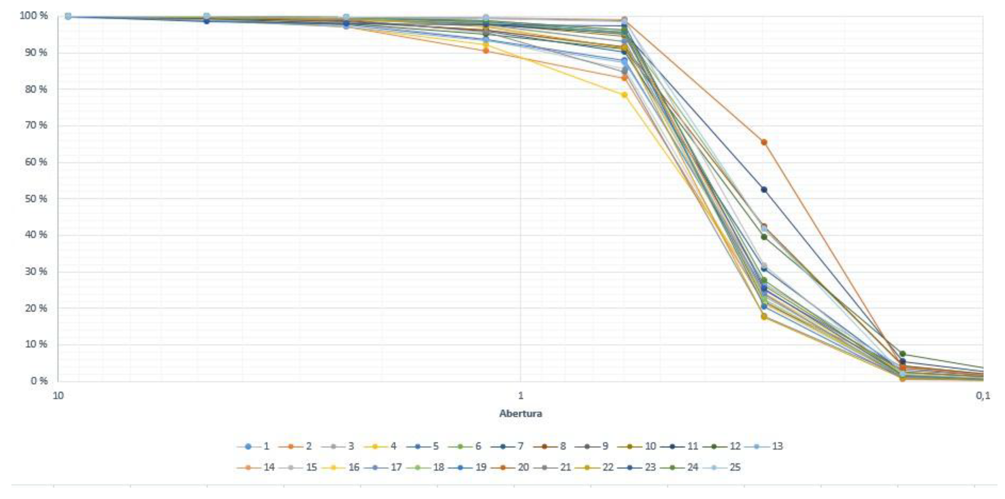
Table 2.
Results of tests performed on fine aggregate (river sand).
| Rehearsal | Average | Standard deviation |
| Percentage of material finer than the 75 µm sieve | 1.44 | 0.61 |
| Apparent density (kg/m3) | 2525.36 | 32.55 |
| Surface-dry saturated density (kg/m3) | 2574.68 | 32.77 |
| Nominal Density (kg/m3) | 2656.77 | 36.38 |
| Absorption (%) | 1.95 | 0.18 |
| Organic matter content | 1 | - |
Source: Own elaboration.
Limestone sand
For each test performed, the mean and standard deviations were found to be used as representative data:
Table 3.
Average limestone granulometry result.
| Sieve | Opening (mm) | Average | Standard deviation |
| 3/8" | 9.5 | 99.99 | 0.073 |
| No. 4 | 4.75 | 94.09 | 0.807 |
| No. 8 | 2.36 | 57.22 | 2,920 |
| No. 16 | 1.18 | 30.46 | 2,267 |
| No. 30 | 0.6 | 20.80 | 1,921 |
| No. 50 | 0.3 | 10.34 | 1,293 |
| No. 100 |
0.15 |
3.50 |
0.701 |
| No. 200 |
0.075 |
1.00 |
0.360 |
Source: Own elaboration.
Fineness modulus: 3.84 ± 0.091
Graph 2.
Granulometric distribution curve of limestone sand. Source: Own elaboration.
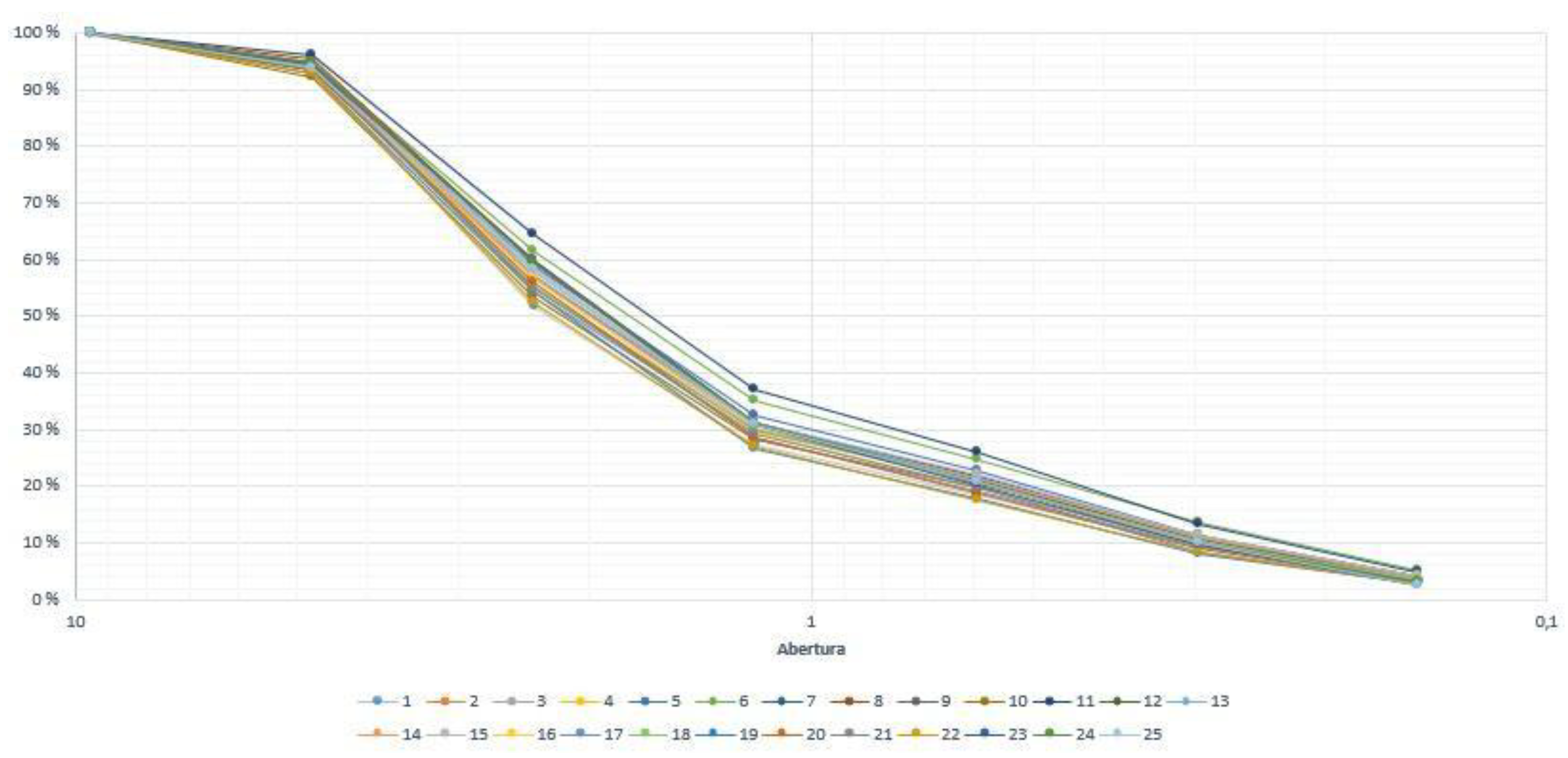
Table 4.
Results of tests performed on fine aggregate (limestone sand).
| Rehearsal | Average | Standard deviation |
| Percentage of material finer than the 75 µm sieve | 6.59 | 0.97 |
| Apparent density (kg/m3) | 2446.46 | 21.87 |
| Surface-dry saturated density (kg/m3) | 2545.63 | 20.83 |
| Nominal Density (kg/m3) | 2716.56 | 24.07 |
| Absorption (%) | 4.05 | 0.21 |
| Organic matter content | 1 | - |
Source: Own elaboration.
Combined Sand
For each test performed, the mean and standard deviations were found to be used as representative data:
Table 5.
Average particle size result of the combined.
| Sieve | Opening (mm) | Average | Standard deviation |
| 3/8" | 9.5 | 99.82 | 0.603 |
| No. 4 | 4.75 | 96.43 | 0.936 |
| No. 8 | 2.36 | 77.04 | 3,242 |
| No. 16 | 1.18 | 61.48 | 5,092 |
| No. 30 | 0.6 | 53.66 | 5,995 |
| No. 50 | 0.3 | 21.26 | 6,063 |
| No. 100 |
0.15 | 3.26 | 1,036 |
| No. 200 |
0.075 | 0.84 | 0.325 |
Source: Own elaboration Fineness modulus: 2.86 ± 0.186.
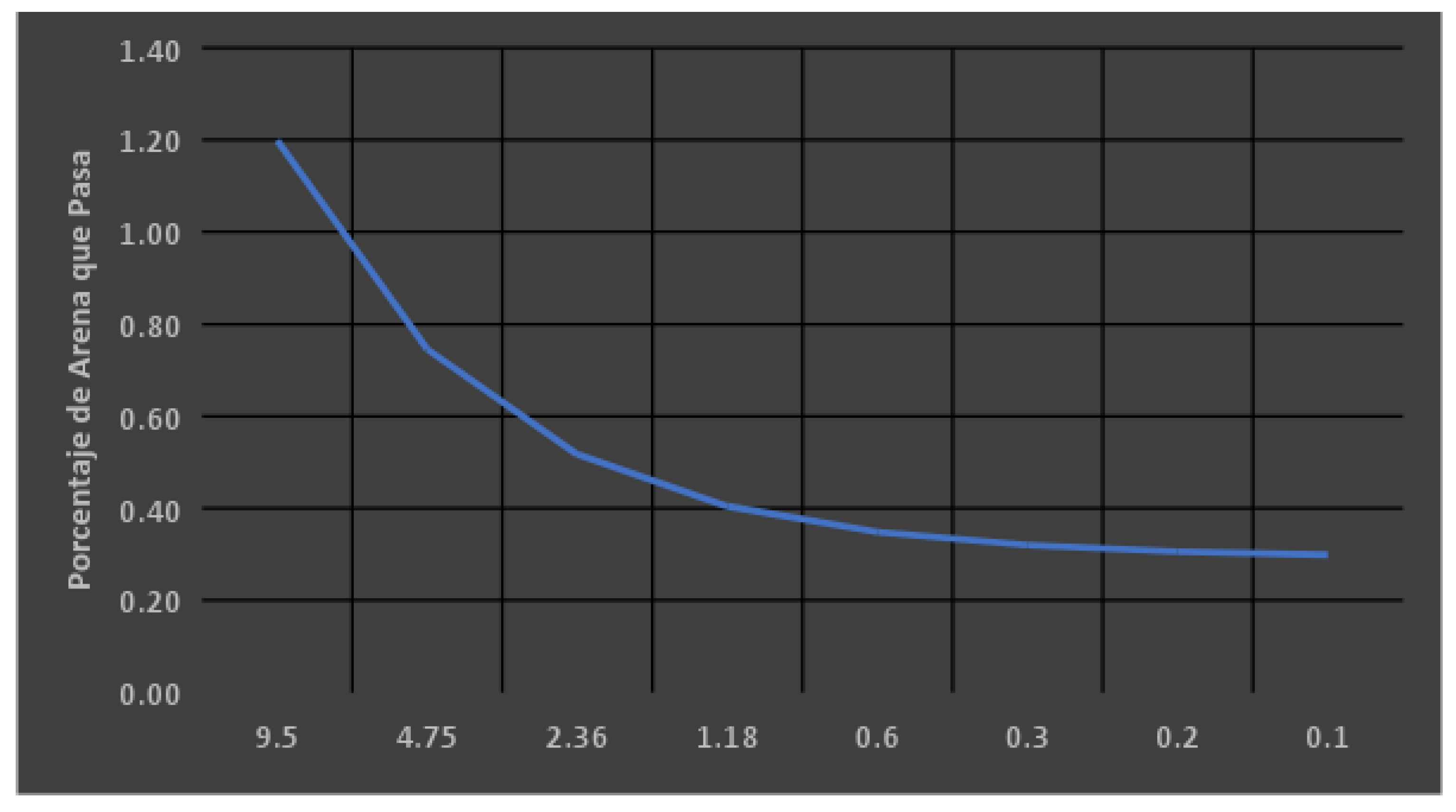
Graph 3.
Granulometric distribution curve of combined sand. Source: Own elaboration.
Table 6.
Results of tests performed on fine aggregate (combined sand).
| Rehearsal | Average | Standard deviation |
| Percentage of material finer than the 75 µm sieve | 3.88 | 0.48 |
| Apparent density (kg/m3) | 2500.53 | 32.40 |
| Surface-dry saturated density (kg/m3) | 2574.68 | 32.77 |
| Nominal Density (kg/m3) | 2701.49 | 40.00 |
| Absorption (%) | 2.97 | 0.29 |
| Organic matter content | 1 | - |
Source: Own elaboration.
Statistical Analysis
Model Adjusted For Rio Sand
The values of the variables X y Y, when the test was carried out with the river sand are shown in the following table:
Table 7.
Values of river sand variables.
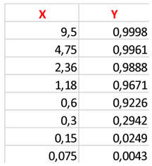 |
Source: Own elaboration.
Using equations (2) and (3), the values of the coefficients are estimated β0 y β, resulting in:
β0 =0.46014208
β =0.0802043
With these values, the linear model that appears in equation (1) is built, resulting in:
𝑌 = 0,46014208 + 0,0802043𝑋 + 𝑒
The values of the coefficients β0 y βare interpreted as follows:
β0 = 0,46014208: When the sieve opening is 0.0 mm, approximately 46.01% of river sand is expected to pass through.
β = 0,0802043For every mm the sieve size increases, the percentage of river sand passing is expected to increase by approximately 8.02%. Alternatively, for every mm the sieve size decreases, the percentage of river sand passing is expected to decrease by approximately 8.02%.
To verify whether this model explains the response variable Y, the corresponding analysis of variance is performed, with which the following hypotheses are tested:
HO : β0 = β = 0“The model does not explain the response variable Y” or “There is no statistically significant relationship between the size of the sieve opening and the percentage of river sand that passes through each sieve.”
Hi: βj ≠ 0“The model does explain the response variable Y” or “There is a statistically significant relationship between the size of the sieve opening and the percentage of river sand that passes through each sieve.”
The results of the analysis of variance are shown in the following table:
Table 8.
Anova.
 |
Source: Own elaboration.
Since the P value = 0.13531205 > α = 0.05, the null hypothesis HO : β0 = β = 0is accepted, there is no statistically significant relationship between the sieve opening size and the percentage of river sand passing through each sieve. Therefore, no further statistical analysis is necessary for this model.
Model Adjusted For Limestone Sand
The values of the variables X y Y, when the test was carried out with the limestone sand are shown in the following table:
Table 9.
Values of the limestone sand variable.
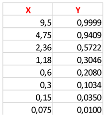 |
Source: Own elaboration.
Using equations (2) and (3), the values of the coefficients are estimated β0 y β, resulting in:
β0 =0.13592128
β =0.11034531
With these values, the linear model that appears in equation (1) is built, resulting in:
𝑌 = 0,13592128 + 0,11034531𝑋 + 𝑒
The values of the coefficients β0 y βare interpreted as follows:
β0 = 0,13592128: When the sieve opening is 0.0 mm, approximately 13.6% of limestone sand is expected to pass through.
β = 0,11034531For every mm increase in sieve size, the percentage of limestone sand passing is expected to increase by approximately 11.03%. Alternatively, for every mm decrease in sieve size, the percentage of limestone sand passing is expected to decrease by approximately 11.03%.
To verify whether this model explains the response variable Y, the corresponding analysis of variance is performed, with which the following hypotheses are tested:
HO : β0 = β = 0“The model does not explain the response variable Y” or “There is no statistically significant relationship between the sieve opening size and the percentage of limestone sand passing through each sieve.”
Hi: βj ≠ 0“The model does explain the response variable Y” or “There is a statistically significant relationship between the size of the sieve opening and the percentage of limestone sand that passes through each sieve.”
The results of the analysis of variance are shown in the following table:
Table 10.
Anova.
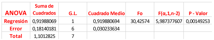 |
Source: Own elaboration.
As the P – Value = 0.00149253≤ α = 0.05The null hypothesis HO: β0 = β = 0is rejected if there is a statistically significant relationship between the sieve opening size and the percentage of limestone sand passing through each sieve. Therefore, it is necessary to perform additional statistical analyses on this model.
The value of R 2 for this model is, R 2 = 0.84, which indicates that the model explains 84% of the variability present in the response variable Y.
The correlation ρbetween the independent and dependent variables is, ρ = 0.91, which indicates that the variables, sieve opening size and percentage of limestone sand that passes, are directly proportional and there is a high relationship of dependence between them.
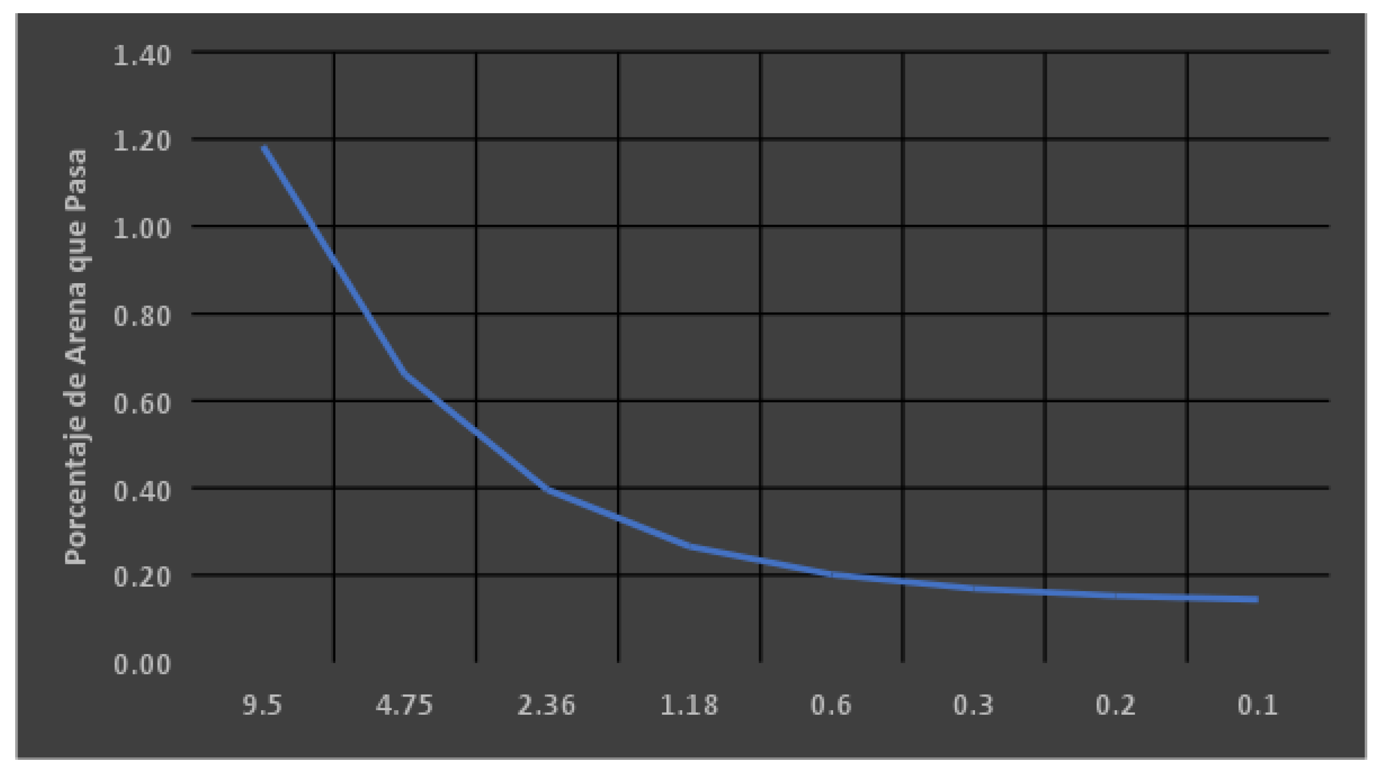
Graph 4.
of the Adjusted Model for the Granulometric Distribution of Limestone Sand Source: Own elaboration.
Graph 4.
of the Adjusted Model for the Granulometric Distribution of Limestone Sand Source: Own elaboration.
Model Adjusted For Combined Sand
The values of the variables X y Y, when the test was performed with the combined sand are shown in the following table:
Table 11.
Combined sand variable values.
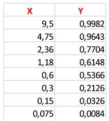 |
Source: Own elaboration.
Using equations (2) and (3), the values of the coefficients are estimated β0 y β, resulting in:
β0 =0.29150871
β =0.09549605
With these values, the linear model that appears in equation (1) is built, resulting in:
Y = 0,29150871 + 0,09549605X + e
The values of the coefficients β0 y βare interpreted as follows:
β0 = 0,29150871: When the sieve opening is 0.0 mm, approximately 29.15% of combined sand is expected to pass.
β = 0,09549605For every mm increase in sieve size, the percentage of combined sand passing is expected to increase by approximately 9.55%. Alternatively, for every mm decrease in sieve size, the percentage of combined sand passing is expected to decrease by approximately 9.55%.
To verify whether this model explains the response variable Y, the corresponding analysis of variance is performed, with which the following hypotheses are tested:
HO : β0 = β = 0“The model does not explain the response variable Y” or “There is no statistically significant relationship between the sieve opening size and the percentage of combined sand passing each sieve.”
Hi: βj ≠ 0“The model does explain the response variable Y” or “There is a statistically significant relationship between the size of the sieve opening and the percentage of combined sand that passes through each sieve.”
The results of the analysis of variance are shown in the following table:
Table 12.
Anova.
 |
Source: Own elaboration.
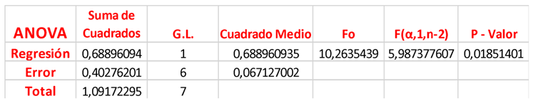
As the P – Value = 0.01851401≤ α = 0.05The null hypothesis HO: β0 = β = 0is rejected if there is a statistically significant relationship between the sieve opening size and the percentage of combined sand passing through each sieve. Therefore, it is necessary to perform additiona l statistical analyses on this model.
The value of R 2 for this model is, R 2 = 0.63, which indicates that the model explains 63% of the variability present in the response variable Y.
The correlation ρbetween the independent and dependent variables is, ρ = 0.79, which indicates that the variables, sieve opening size and percentage of combined sand that passes, are directly proportional and there is a high relationship of dependence between them.
Graph 5.
Adjusted Model for the Granulometric Distribution of the Combined Sand Source: Own elaboration.
Graph 5.
Adjusted Model for the Granulometric Distribution of the Combined Sand Source: Own elaboration.
Analysis of Results
Table 13.
Results of the average compressive strength at 28 days of the concrete specimens for different A/C ratios.
Table 13.
Results of the average compressive strength at 28 days of the concrete specimens for different A/C ratios.
| A/C | Age (Days) | Average strength (MPa) | Standard Deviation |
| 0.75 | 28 | 15.90 | 3.04 |
| 0.7 | 28 | 24.99 | 2.67 |
| 0.65 | 28 | 28.38 | 2.56 |
| 0.6 | 28 | 28.80 | 3.24 |
| 0.55 | 28 | 36.39 | 3.40 |
| 0.5 | 28 | 39.67 | 3.18 |
| 0.45 | 28 | 45.81 | 4.67 |
| 0.4 | 28 | 55.29 | 4.68 |
| 0.35 | 28 | 59.52 | 8.29 |
Source: Own elaboration.
Table 14.
Results of the average compressive strength at 7 days of the concrete specimens for different A/C ratios.
Table 14.
Results of the average compressive strength at 7 days of the concrete specimens for different A/C ratios.
| A/C | Age (Days) | Average strength (MPa) | Standard Deviation |
| 0.75 | 7 | 14.07 | 3.46 |
| 0.7 | 7 | 19.22 | 3.88 |
| 0.65 | 7 | 22.25 | 3.23 |
| 0.6 | 7 | 24.44 | 5.23 |
| 0.55 | 7 | 31.24 | 1.56 |
| 0.5 | 7 | 33.22 | 1.78 |
| 0.45 | 7 | 41.16 | 6.52 |
| 0.4 | 7 | 51.99 | 5.47 |
| 0.35 | 7 | 55.74 | 9.69 |
Source: Own elaboration.
Table 15.
Average percentage of compressive strength reached at 7 days of age with respect to the average strength reached at 28 days of age, for different A/C ratios.
Table 15.
Average percentage of compressive strength reached at 7 days of age with respect to the average strength reached at 28 days of age, for different A/C ratios.
| A/C | 7-day average (MPa) | Average 28 days (MPa) | Percentage Achieved 7 days (%) |
| 0.75 | 13.54 | 15.65 | 86.51 |
| 0.7 | 19.22 | 24.23 | 79.30 |
| 0.65 | 22.25 | 27.82 | 79.97 |
| 0.6 | 24.44 | 28.66 | 85.28 |
| 0.55 | 31.24 | 36.52 | 85.53 |
| 0.5 | 33.22 | 39.67 | 83.74 |
| 0.45 | 38.25 | 46.01 | 83.14 |
| 0.4 | 48.44 | 54.59 | 88.74 |
| 0.35 | 50.99 | 59.19 | 86.15 |
| Average | 84.26 |
Source: Own elaboration.
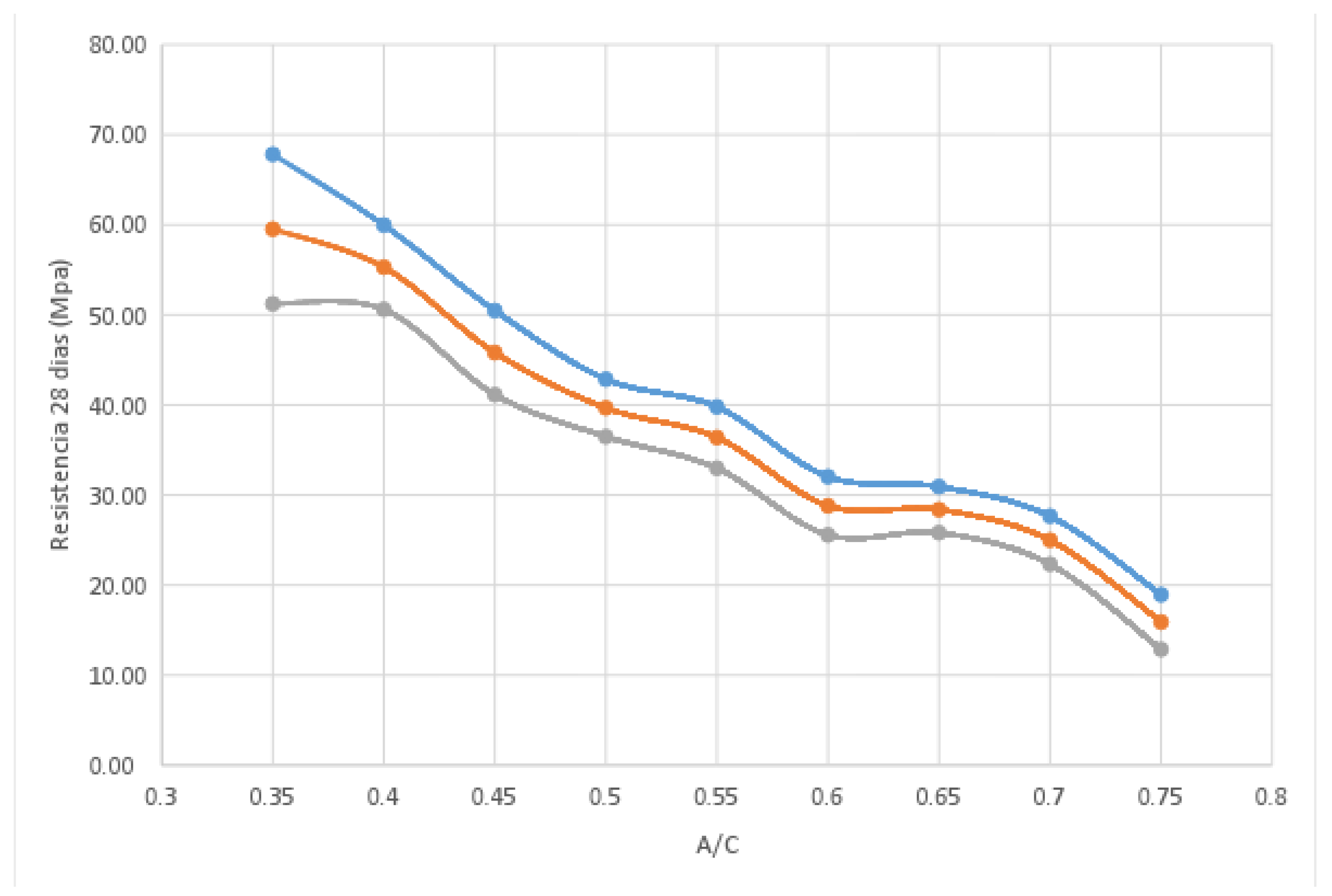
Preparation and Modeling of the A/C Curve
From the data collected previously, it is possible to construct the curve taking into account the variables A/C ratio on the abscissas and Compressive strength at 28 days on the ordinates. The following table shows the average strength data obtained, as well as their respective standard deviations:
Table 16.
Results of the average compressive strength at 28 days of the concrete specimens for different A/C ratios.
Table 16.
Results of the average compressive strength at 28 days of the concrete specimens for different A/C ratios.
| A/C | Age (Days) | Average strength (MPa) | Standard Deviation |
| 0.75 | 28 | 15.90 | 3.04 |
| 0.7 | 28 | 24.99 | 2.67 |
| 0.65 | 28 | 28.38 | 2.56 |
| 0.6 | 28 | 28.80 | 3.24 |
| 0.55 | 28 | 36.39 | 3.40 |
| 0.5 | 28 | 39.67 | 3.18 |
| 0.45 | 28 | 45.81 | 4.67 |
| 0.4 | 28 | 55.29 | 4.68 |
| 0.35 | 28 | 59.52 | 8.29 |
Source: Own elaboration.
Table 17.
Results of average compressive strength, standard deviation, and upper and lower limits at 28 days of concrete specimens for different W/C ratios.
Table 17.
Results of average compressive strength, standard deviation, and upper and lower limits at 28 days of concrete specimens for different W/C ratios.
| A/C | Average strength (Mpa) |
Deviation | upper limit (Mpa) | upper limit (Mpa) |
| 0.75 | 15.90 | 3.04 | 18.94 | 12.87 |
| 0.7 | 24.99 | 2.67 | 27.66 | 22.33 |
| 0.65 | 28.38 | 2.56 | 30.93 | 25.82 |
| 0.6 | 28.80 | 3.24 | 32.04 | 25.57 |
| 0.55 | 36.39 | 3.40 | 39.79 | 32.98 |
| 0.5 | 39.67 | 3.18 | 42.85 | 36.49 |
| 0.45 | 45.81 | 4.67 | 50.48 | 41.14 |
| 0.4 | 55.29 | 4.68 | 59.97 | 50.61 |
| 0.35 | 59.52 | 8.29 | 67.82 | 51.23 |
Source: Own elaboration.
Graph 6.
A/C ratio curve Source: Own elaboration.
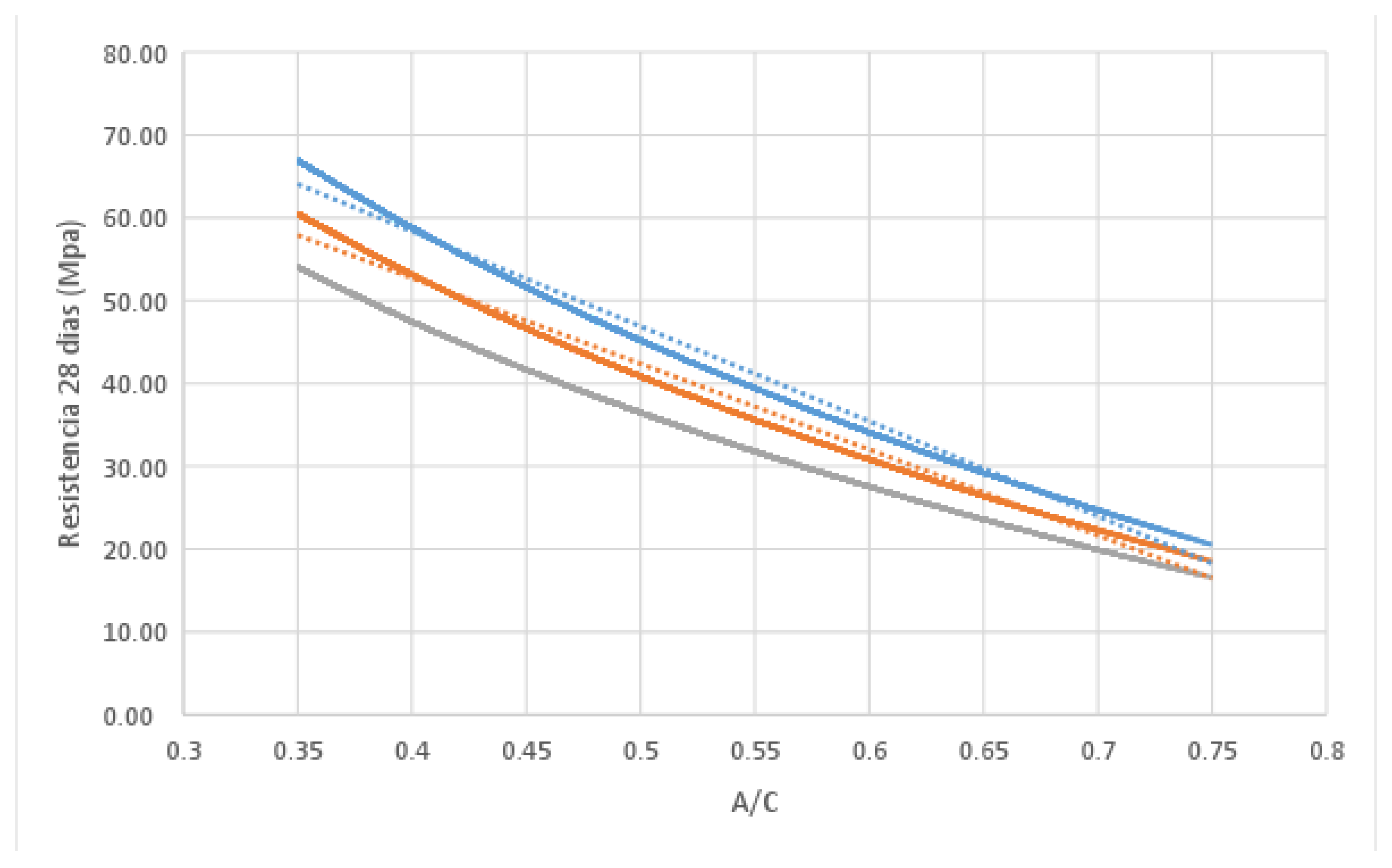
The type of function that was presented as the best option for modeling the curve obtained was the logarithmic one; when applying the modeling, the final graph is the following:
Figure 7.
Modeling the A/C ratio curve created by a logarithmic trend line in a scatter plot in Excel. Source: Own elaboration.
Figure 7.
Modeling the A/C ratio curve created by a logarithmic trend line in a scatter plot in Excel. Source: Own elaboration.
Conclusions
The optimization of the proportions of the combined sand was possible thanks to the graphic method proposed by RNL, obtaining combination percentages that were not
very viable for the in situ composition of the combined sand, so the combination used by the company was theoretically optimized, but due to the mixing processes of these two sands, the 50-50 ratio was maintained, which meets the technical specifications for use as fine material in concrete.
Mix designs using the ACI method, varying the A/C ratios, allowed us to know the resistance values that the concrete could offer, allowing the development and modeling of the A/C curve.
The expected reliability was met by most of the cylinders tested, only two of the checked specimens being outside showing a resistance in excess of the expected one, that is, the objective of reaching a reliability of 85% in the compressive strength of the concrete mix designs was achieved as shown in the results obtained.
The materials used in the concrete company are capable of obtaining high-strength concrete designs, a point in favor of the development of construction materials for our municipality.
The optimization of the mix designs based on the data obtained from our curve was achieved, showing higher A/C ratios for the same strength than those provided by the company supporting the research. However, it should be noted that, according to the company's reports, its curve is subject to optimization by additives, unlike ours, which makes the most of the materials used by the concrete plant. The lowest strengths of 14 and 17.5 are outside the experimentally checked limits; these were obtained through the mathematical model presented in the curve, so the relevant checks must be performed.
References
- Bracamonte Miranda, A. J., Vertel Morinson, M. L., & Cepeda Coronado. (2013). Caracterización Físico-mecánica de agregados peteros de la formación geológica Toluviejo (Sucre) para producción de concreto.
- Ávila Díaz, M. Á., Galviss Pizon, S., & Serna Hernández, L. F. (2015). Análisis de curvas para el diseño de mezclas de concreto con material triturado del río Magdalena en el sector de Girardot, Cundinamarca.
- Orbe Pinchao, L. V., & Zúñiga Morales, P. S. (2013). Optimización de la relación agua/cemento en el diseño de hormigones estándar establecidos en códigos ACI-ASTM.
- Sánchez, D. (1997). Tecnología de concreto – Tomo 1. Bhandar Editores Ltda.
- Valdivieso Taborda, C. E., Valdivieso Castellón, R., & Valdivieso Taborda, O. (2011).
- Determinación de muestra bajo el árbol de decisión.
- Instituto Colombiano de Normas Técnicas y Certificación (ICONTEC). NTC 129: Ingeniería Civil y Arquitectura. Práctica para la toma de muestras de agregados.
- Instituto Colombiano de Normas Técnicas y Certificación (ICONTEC). NTC 3674: Ingeniería civil y Arquitectura. Práctica para la reducción de las muestras de agregados, tomadas en campo para la realización de ensayos.
- Instituto Colombiano de Normas Técnicas y Certificación (ICONTEC). (2000). NTC 174: Concretos: Especificaciones de los agregados para el concreto.
- Instituto Colombiano de Normas Técnicas y Certificación (ICONTEC). (2007). NTC 77: Concretos: Método de ensayo para el análisis por tamizado de los agregados finos y gruesos.
- Instituto Colombiano de Normas Técnicas y Certificación (ICONTEC). NTC 1776: Ingeniería civil y Arquitectura. Método de ensayo para determinar por secado el contenido total de humedad de los agregados.
- Instituto Nacional de Vías (INV). INV E-230: Índice de aplanamiento y alargamiento de los agregados para carreteras.
- Instituto Colombiano de Normas Técnicas y Certificación (ICONTEC). (2000). NTC 176: Ingeniería Civil y Arquitectura: Método para determinar la densidad y absorción del agregado grueso.
- Instituto Colombiano de Normas Técnicas y Certificación (ICONTEC). (1995). NTC 92: Ingeniería Civil y Arquitectura: Determinación de la masa unitaria y los vacíos entre partículas de agregados.
- Instituto Colombiano de Normas Técnicas y Certificación (ICONTEC). (1995). NTC 78: Ingeniería Civil y Arquitectura: Método para determinar por lavado el material que pasa el tamiz 75 µm en agregados minerales.
- Instituto Colombiano de Normas Técnicas y Certificación (ICONTEC). (2000). NTC 237: Ingeniería Civil y Arquitectura: Método para determinar la densidad y absorción del agregado fino.
- Instituto Colombiano de Normas Técnicas y Certificación (ICONTEC). (2000). NTC 127: Concretos: Método de ensayo para determinar las impurezas orgánicas en agregado fino para concreto.
- Instituto Colombiano de Normas Técnicas y Certificación (ICONTEC). (1992). NTC 396: Ingeniería Civil y Arquitectura: Método de ensayo para determinar el asentamiento del concreto.
- Instituto Colombiano de Normas Técnicas y Certificación (ICONTEC). (1994). NTC 1377: Ingeniería Civil y Arquitectura: Elaboración y curado de especímenes de concreto para ensayos de laboratorio.
- Instituto Colombiano de Normas Técnicas y Certificación (ICONTEC). NTC 3512: Cementos. Cuartos de mezclado, cámaras y cuartos húmedos y tanques para el almacenamiento de agua, empleados en los ensayos de cementos hidráulicos y concretos.
- Instituto Colombiano de Normas Técnicas y Certificación (ICONTEC). (2010). NTC 673: Concretos: Ensayo de resistencia a la compresión de especímenes de concreto.
- American Concrete Institute (ACI). (2011). Código ACI 318-11: Requisitos de reglamento para concreto estructural.
- ASOCRETO. (s. f.). Tecnología del Concreto, Tomo 1, Cap. 8.
Disclaimer/Publisher’s Note: The statements, opinions and data contained in all publications are solely those of the individual author(s) and contributor(s) and not of MDPI and/or the editor(s). MDPI and/or the editor(s) disclaim responsibility for any injury to people or property resulting from any ideas, methods, instructions or products referred to in the content. |
© 2025 by the authors. Licensee MDPI, Basel, Switzerland. This article is an open access article distributed under the terms and conditions of the Creative Commons Attribution (CC BY) license (http://creativecommons.org/licenses/by/4.0/).
Copyright: This open access article is published under a Creative Commons CC BY 4.0 license, which permit the free download, distribution, and reuse, provided that the author and preprint are cited in any reuse.


