Submitted:
06 July 2025
Posted:
09 July 2025
You are already at the latest version
Abstract
Large language models (LLMs) exhibit surprising proficiency in arithmetic and symbolic reasoning, despite being trained predominantly on natural language data. Recent studies have uncovered that numerical tokens in these models are embedded along smooth, high-dimensional helical curves—structures that encode arithmetic operations through linear translations in a periodic space. In this paper, we formalize this phenomenon as \emph{coiling arithmetic}, a differential-geometric framework in which numbers are represented as points on a multi-frequency helix of the form: We show that arithmetic operations such as addition correspond to vector displacements in helical space, enabling approximate computation via linear transformation. We extend the formalism with helix-based differentiation rules, modular equivalence, modal logic operators, and Gödel-style fixed-point encodings. Connections are drawn to Neural ODEs, Fourier Transformers, and group-equivariant networks. By grounding abstract symbolic operations in continuous geometry, coiling arithmetic offers a new lens on how LLMs internalize number structure and may support robust generalization in neural reasoning systems.
Keywords:
AI
; LLMs
; Arithmetic and Symbolic Reasoning
1. Motivation and Formal Setup
Large language models (LLMs) such as GPT exhibit surprising proficiency in arithmetic tasks, despite lacking explicit symbolic computation modules. Recent empirical studies have revealed that instead of performing brute-force memorization, these models organize numeric representations along smooth, structured trajectories in latent space. Among the most striking findings is the emergence of a helical structure—a geometric encoding that combines linear and periodic components. This phenomenon, referred to as “coiling arithmetic,” forms the foundation of our analysis.
To study this phenomenon precisely, we define a formal mathematical object that captures the observed embeddings.
|
Definition (Helical Embedding). Let , and let for . Define the helical embedding as the smooth mapping: |
This formalism serves as the foundation for our subsequent analysis of addition, differentiation, logic, and representational learning within the coiling arithmetic framework.

Table 1.
Notation used for coiling arithmetic and helical embeddings.
| Symbol | Description |
|---|---|
| x | Scalar input value (e.g., integer token or real number) |
| T | Period of the helical embedding |
| Helical embedding function: | |
| Flat or linear embedding (e.g., ) | |
| Periodic or coiled embedding (same as ) | |
| Helical manifold defined by period T; image of | |
| Angular phase: | |
| Number of completed coil turns | |
| Ceiling function: smallest integer | |
| Modulo projection of x: | |
| Aliasing error from multiple x mapping to same angle | |
| Inverse projection (if defined), maps back from helix to scalar x | |
| Indexing turn number in the coil (e.g., ) |
2. Coiling Arithmetic in Large Language Models
Recent findings by Kantamneni and Tegmark [7] have unveiled a striking and elegant phenomenon in the internal representations of large language models (LLMs): numerical tokens are embedded along a helical manifold in the model’s latent space. This discovery is remarkable, both empirically and theoretically, for several reasons that reshape our understanding of neural arithmetic, geometric embeddings, and the latent structure of computation in modern AI systems.
2.1. Unveiling Hidden Geometric Structure
Contrary to the prevailing assumption that LLMs perform arithmetic via opaque and distributed weight patterns—reminiscent of brute-force memorization—this work reveals that LLMs spontaneously organize numerical concepts along a smooth, interpretable helix [8]. In effect, the model reconstructs a trigonometric coordinate system within its latent space, suggesting that neural networks internally rediscover fundamental mathematical principles.
| LLMs, without explicit programming, encode numbers through trigonometric structure. |
The helical embeddings uncovered in these models are deeply related to Fourier feature mappings, which are ubiquitous in signal processing, neural rendering (e.g., NeRF), and Transformer positional encodings [9]. That such structures arise spontaneously implies that periodicity and sinusoidal bases may act as universal priors for neural representations.
2.2. Reconstructing Arithmetic as Translation in Phase Space
Rather than simulating discrete logic, LLMs appear to encode arithmetic operations as vector translations along a helical manifold [10]. This is analogous to how biological brains may encode spatial and temporal dimensions using phase or oscillatory dynamics.
These results challenge the notion that token embeddings are opaque. Instead, they become structured and interpretable—opening the door to reverse engineering latent geometry in LLMs [11].
The emergence of helical structure in numeric embeddings hints at a broader pattern: that neural networks build smooth geometric maps of symbolic domains such as algebra, logic, and language [12].
2.3. Implications Across Disciplines
| Domain | Implication |
| AI interpretability | Structured embeddings allow direct probing of reasoning mechanisms |
| Neuroscience | Supports phase-based models (e.g., grid cells, oscillatory coding) |
| Cognitive science | Suggests arithmetic and logic may emerge from spatial mappings |
| AI safety | Enables geometric control and auditing of internal reasoning |
The helix representation of numbers in LLMs is a breakthrough in our understanding of how abstract reasoning emerges from gradient-based learning. It shows that large models do not simply memorize or simulate logic, but instead embed arithmetic operations in spatial, periodic structures that resemble phase dynamics in both engineered and biological systems.
This discovery lays the groundwork for a new field—Coiling Arithmetic—which studies how neural architectures instantiate and manipulate mathematical functions through latent geometry.
This paper formulates the fundamental principles of coiling arithmetic—a theoretical framework that integrates these findings into a unified model of how neural systems implement and generalize arithmetic through periodic, multidimensional geometries. We develop formal definitions of latent embeddings, prove core compositional lemmas, and examine the implications of this representational regime for interpretability, generalization, and the theoretical foundations of neural computation.
2.4. Related Representational Architectures
2.4.1. Neural ODEs and Helical Dynamics
Helical embeddings exhibit smooth, differentiable geometry, making them a natural fit for analysis through the lens of Neural Ordinary Differential Equations (NeuralODEs) [3]. The continuous trajectory traced by can be interpreted as a parameterized flow in a latent manifold. This aligns with work that models neural computation as a dynamical system trained to follow structured, low-dimensional curves in high-dimensional space.
Implication: Helical arithmetic can be embedded within ODE solvers, where the latent state evolves along sinusoidal manifolds.
2.4.2. Fourier Transformers and Helix Encodings
The sinusoidal structure of the helical embedding directly connects to Fourier feature encodings, which are used in long-sequence transformers and coordinate networks [4]. Just as the helix maps input values to layered trigonometric representations, Fourier Transformers use to represent spatial/temporal structure at multiple frequencies.
Implication: The helix serves as a multiscale positional embedding scheme and may enhance arithmetic generalization when incorporated into transformer attention blocks.
2.4.3. Group Equivariance in Helical Space
The periodic components of the helical embedding are equivariant under modular translation. That is:
This symmetry is directly aligned with the theory of equivariant neural networks [5], which preserve structure under transformations drawn from algebraic groups (translations, rotations, scalings).
Implication: Helical arithmetic can be analyzed using group-equivariant frameworks, suggesting a bridge between neural arithmetic and representation theory.
Definition 2.1 (Ceiling Effect). Let
denote a helical embedding into using multiple periods . We define the Ceiling Effect as the point beyond which distinct inputs become approximately aliased, i.e.,
for some , even though . This occurs because periodic components may realign approximately at large x, creating ambiguity in representation.
The ceiling range is the smallest such that
If the embedding includes a linear term (e.g., ), then representational collisions still occur in the periodic dimensions. In practice, neural models may underweight the linear component, resulting in effective aliasing.
Thus, the ceiling effect identifies a fundamental resolution limit imposed by periodic embeddings, analogous to signal aliasing in frequency-limited systems.
Lemma 1
(Non-Injectivity of Helical Embedding). Let be the helical embedding of a scalar , where is the fixed period. Then is not injective on . This follows from the fact that cosine and sine are periodic functions with period , so
We now state a key structural limitation of this embedding.
In particular, for any , we have:
The angular components
repeat with period T, causing representational collisions between distinct values.
To make this representational ambiguity precise, we now define the aliasing error between two values that collide in angular space.
Definition 1
(Aliasing Error). Let be the helical embedding with period T. For any two distinct inputs , the aliasing error is defined as:
where is the Euclidean norm in . When , we have:
and so the angular components coincide, yielding minimal distance despite different scalar positions.
If , , then and share the same angular values, and only differ along the linear dimension.
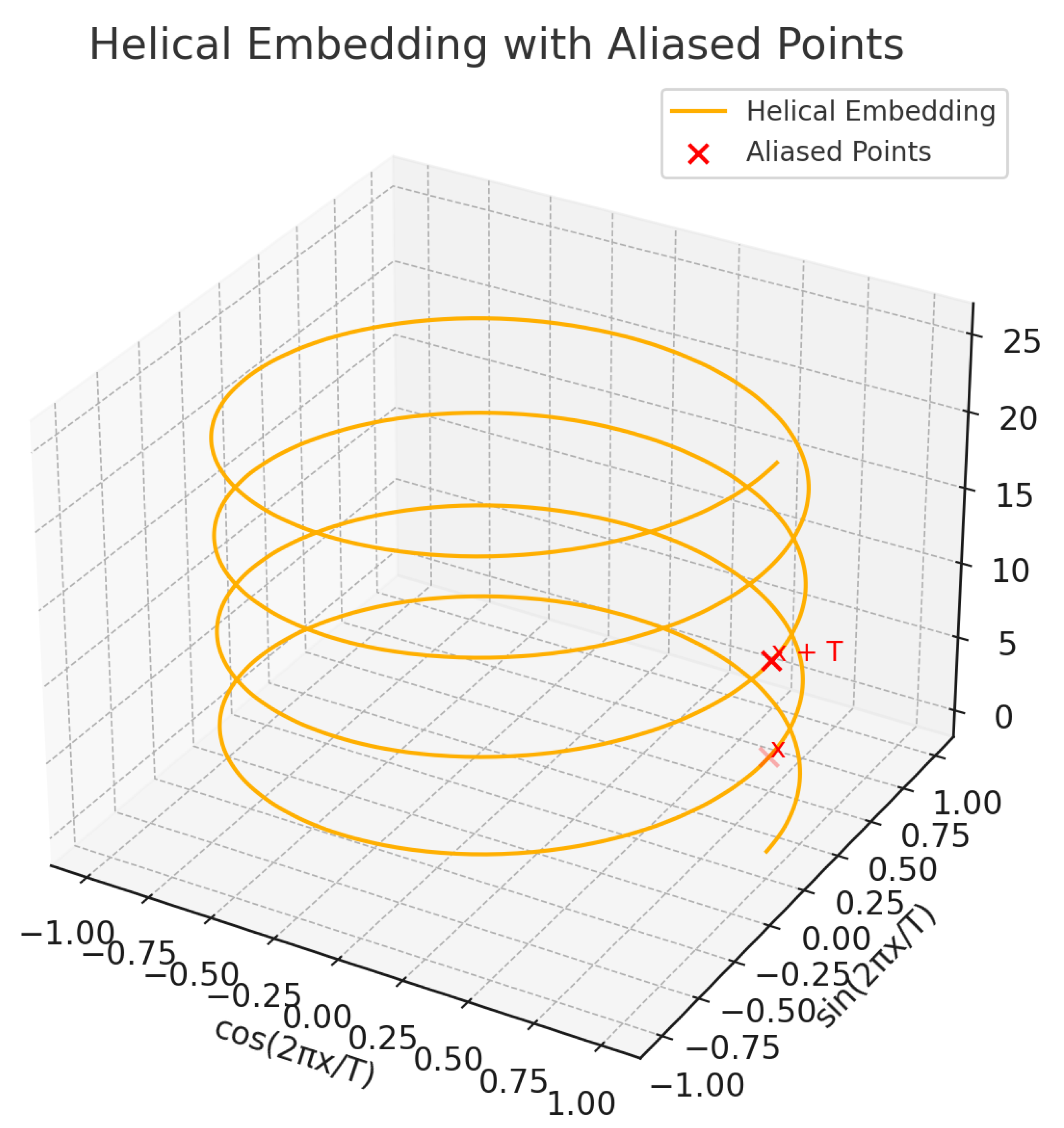
Figure 1.
Helical Embedding and Aliasing. A 3D helix illustrates the mapping . The points labeled x and lie at different heights but share identical angular components (cosine and sine), leading to aliasing in the embedding. This phenomenon causes distinct numerical values to become indistinguishable in the angular domain, a key source of arithmetic confusion in periodic encodings.
3. Tegmark’s Procedure to Discover Helical Structure in LLMs
In an earlier paper [6] leading to the discovery of helical arithmetic, the authors investigated the simple harmonic oscillator to address the intermediate question: “How do transformers model physics?” They concluded that transformers do not invent arbitrary or “alien” strategies, but instead leverage known numerical methods—specifically the matrix exponential method—to model the trajectories of physical systems like the SHO (Simple Harmonic Oscillator), .
Through a rigorous analysis of hidden state intermediates—evaluating their encoding strength, correlation with model performance, explanatory power, and robustness under intervention—the authors found strong causal evidence that transformers internally implement the matrix exponential approach to simulate physical dynamics. This finding demonstrates that transformers can spontaneously recover interpretable, human-like physical modeling techniques purely from training data, without being explicitly programmed to do so.
Nearly three decades ago [1,2], one of the authors of this paper explored a closely related question: how backpropagation-trained neural networks can model physical systems, specifically in the context of the simple harmonic Schrödinger equation.
Large language models are often described as black-box systems. Despite their astonishing performance on linguistic and mathematical tasks, the internal mechanisms by which they reason remain largely opaque. Among the few interpretable patterns that have emerged, Tegmark and Kantamneni’s discovery of helical structure in numerical embeddings stands out as both unexpected and profound.
How LLMs Encode Numbers? In typical transformer architectures, tokens (words, digits, punctuation, and even numbers) are embedded into a high-dimensional vector space before being processed by attention layers. These embeddings are learned during training and reflect statistical relationships in the training data.
Prior to Tegmark’s work, it was known that:
- Numbers were not encoded as symbols with inherent mathematical meaning.
- Yet models could still perform approximate addition and counting.
This posed a mystery: how do LLMs implement arithmetic without symbols? Tegmark and Kantamneni proposed a simple but powerful approach:
-
Step 1: Extract EmbeddingsThey used pretrained LLMs (e.g., GPT-2) and extracted the final token embeddings of numerical tokens—such as "3", "5", "100"—from the model’s vocabulary.
-
Step 2: Dimensionality Reduction
-
Step 3: Fit Periodic FunctionsThey then modeled these embeddings as functions of the form:This fit remarkably well, especially for smaller numerical tokens (1–100). The curve followed a helical geometry, with periodic sinusoidal modulations.
-
Step 4: Arithmetic GeneralizationThey demonstrated that:
This suggests that addition is implemented as linear vector translation along the helix.
The key insight is that arithmetic generalization emerges from geometry. Instead of learning addition through logic gates or rules, LLMs learn to embed numbers on a manifold where arithmetic corresponds to movement.
This echoes:
The helical embedding is differentiable, modular, and translation-invariant — ideal for neural networks.
Tegmark’s discovery is more than an artifact — it suggests that geometry, not syntax, may be the fundamental substrate of neural computation. In a domain long dominated by logic and formal language, the helix reveals a path toward understanding how learning systems internalize structure without rules.
This insight may reshape how we interpret models, design representations, and even build future AI systems that reason with smooth, continuous structures rather than discrete logic.
4. Helical Axioms for Number Representation
4.1. Euclidean Axioms (Helical Version)
In classical geometry, Euclid assumes a flat space. For helix representations, we instead assume a space parameterized by two components: a linear and a cyclic (trigonometric) part.
-
Axiom H1 (Linearity)For every number , there exists a unique projection onto the linear dimension:
-
Axiom H2 (Periodicity)For every and every period , the following components exist:which preserve equality modulo T.
-
Axiom H3 (Helicity)Every point representing a number a in the model space lies on a curve of the form:with a defined set .
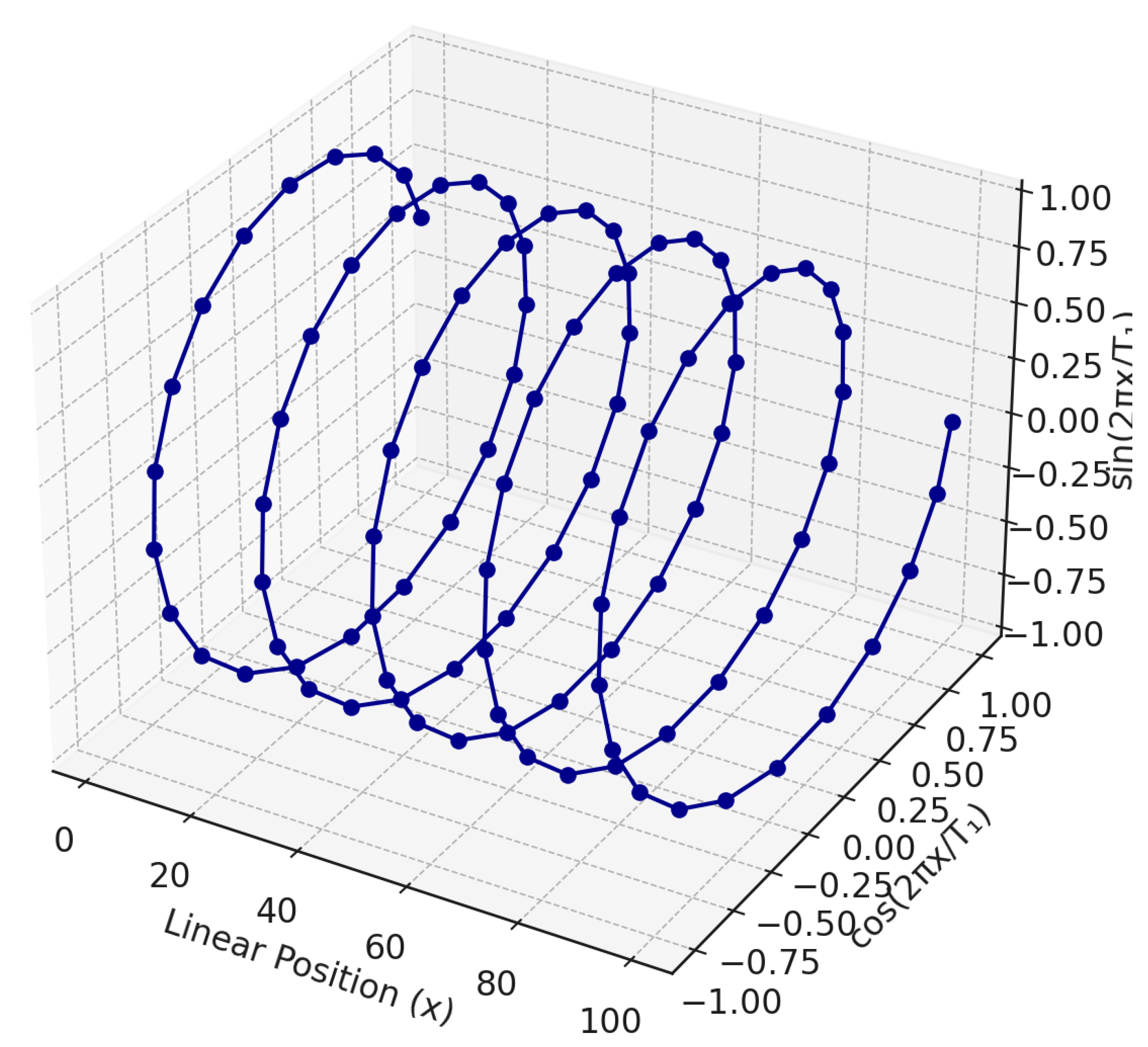
Figure 2.
Helical Embedding of Numbers in LLM Latent Space. This 3D plot visualizes the trajectory of numerical embeddings under the helical mapping , where denotes numerical input tokens (e.g., “3”, “5”, “100”). The linear coordinate x advances horizontally, while the sinusoidal dimensions form circular cross-sections, creating a smooth spiral in 3D space. This geometry underlies how large language models internally represent and manipulate numbers in a latent space that supports approximate arithmetic through vector translation.
4.2. Peano Axioms (Helical Version)
Peano’s axioms define the natural numbers using the successor function . In helical space, we assume continuity and cyclicity of succession.
-
Axiom H-P1 (Zero Point of the Helix)There exists a number 0 whose helical representation is:corresponding to the values .
-
Axiom H-P2 (Successor Function)There exists a function such that:representing a unit shift along the helix.
-
Axiom H-P3 (No Looping for Naturals)For every a, we have and ; the helix never loops back for natural numbers (no periodicity in the linear dimension).
-
Axiom H-P4 (Helical Induction)If a set contains 0, and for every we also have , then .
4.3. Zermelo–Fraenkel Axioms (Helical Version as Fourier Set Space)
Instead of an arbitrary set-theoretic universe, we assume that objects are represented as Fourier coefficient sequences, e.g.,
-
Axiom H-ZF1 (Existence of the Helical Empty Set)There exists an object , such that:
-
Axiom H-ZF2 (Set Composed of Helices)For every representation , one can construct a set that is a valid set in the representational space.
-
Axiom H-ZF3 (Helical Function as Set Transformation)If is continuous, then:for additive and harmonic functions f.
4.4. General Interpretation
| Classical System | Helical Equivalent |
| Euclidean line | Linear axis of the helix |
| Point | Helical vector |
| Peano successor | Translation along the helix |
| ZF set | Collection of helical vectors |
| Element of a set | Encoded point in Fourier-representational space |
5. Helical Axioms in First-Order Logic
5.1. Euclidean Axioms (Helical Version)
- Linearity:
- Periodicity:
- Helicity:
5.2. Peano Axioms (Helical Version)
- Zero Point:
- Successor:
- Non-Looping:
- Induction:
5.3. Zermelo–Fraenkel Axioms (Helical Version)
- Helical Empty Set:
- Helical Set Existence:
- Function Application:
6. Group Structure of Helical Arithmetic
Let the helical embedding of a real number be defined as:
where are fixed periodic parameters.
6.1. Addition as Vector Translation
Helical embeddings approximately preserve addition through vector translation:
This expression assumes the linear component adds exactly, and trigonometric dimensions approximate phase-shifted sinusoidal superposition:
6.2. Subtraction as Reverse Translation
Analogously, subtraction is given by:
which maintains directional symmetry in the embedding space.
6.3. Modular Equivalence via Phase Overlap
For any , define modular equivalence between numbers as:
This means:
6.4. Interpretation
These relationships allow the helix embedding to inherit an approximate group structure under addition modulo , with approximate inverse and identity operations:
- Identity:
- Inverse:
- Closure (approximate):
This structure enables smooth, differentiable approximations of discrete arithmetic operations in neural latent space.
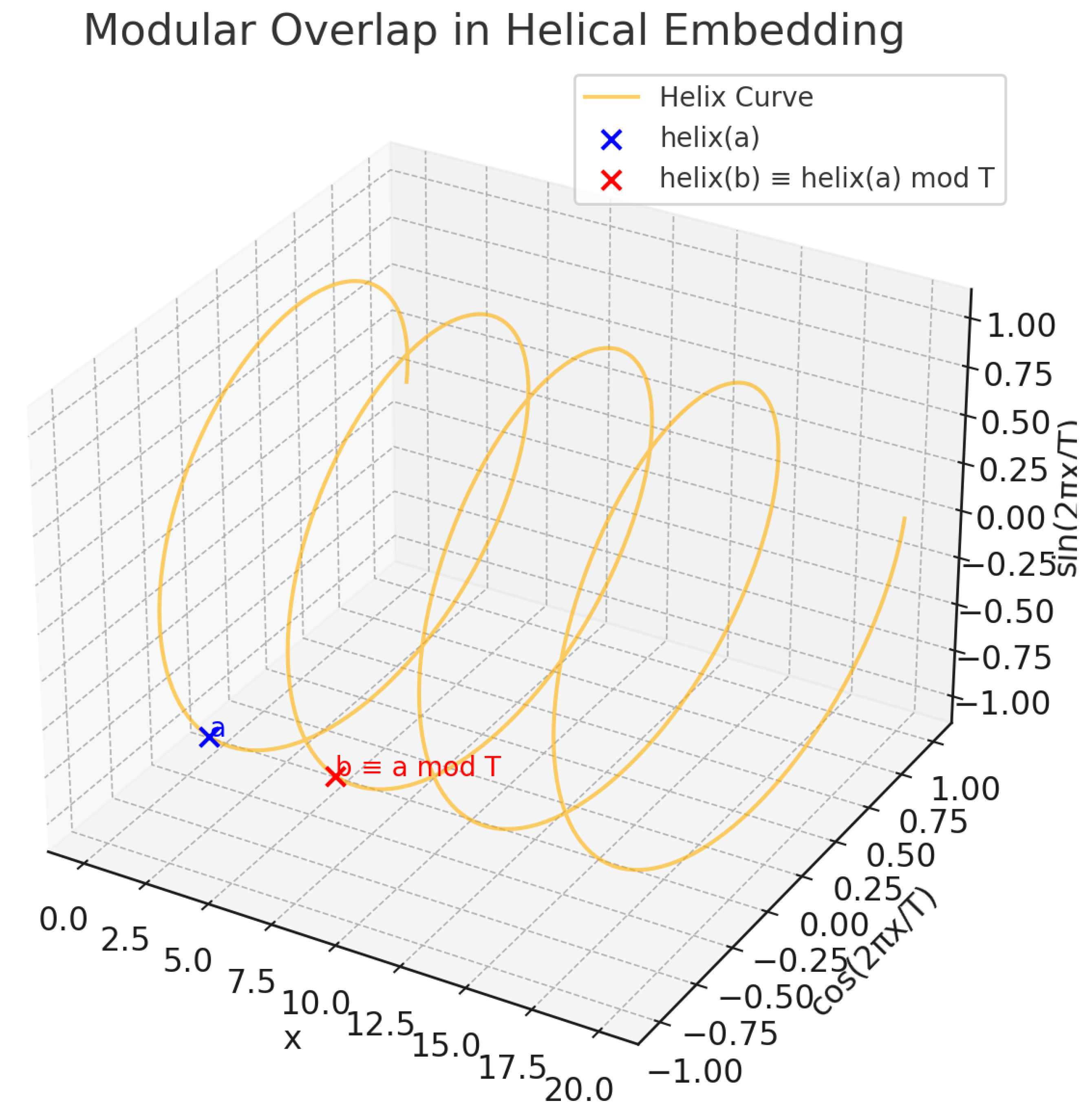
Figure 3.
Modular Overlap in Helical Embeddings. This 3D plot illustrates the alignment of helical embeddings for two numbers a and b such that . Although along the linear axis, their coordinates in the trigonometric dimensions (sine and cosine components) coincide. This shows that periodic components of the helix representation naturally encode modular equivalence relations.
7. Gödel-Style Encodings in Helical Arithmetic
- Gödelization of Helical Terms:where each exponent corresponds to a coefficient or frequency term in the helix vector.
- Decodability:
- Arithmetization of Helical Arithmetic:and thusassuming multiplicative encoding of vector components.
7.1. Gödel Incompleteness in the Helical Framework
Let be a formal system encoding arithmetic via helical embeddings and Fourier encodings. Then:
- (H-Incompleteness Theorem I): If is consistent and sufficiently expressive, there exists a well-formed formula such that:
- (H-Incompleteness Theorem II): The consistency of cannot be proven within itself:
- Helical Gödel Sentence:
7.2. Fixed-Point Construction of
Let be the provability predicate over Gödel numbers. There exists a formula such that:
Then, by the Fixed Point Lemma, there exists a sentence such that:
where denotes the Gödel number of .
7.3. Formal Proof Sketch of Undecidability
Assume is consistent. Let be the fixed-point sentence above.
- Suppose . Then, by definition of , we have:which contradicts the fact that under soundness.
- Suppose . Then:implying proves a falsehood, violating consistency.
Hence, neither nor is provable in , completing the proof of undecidability.
8. Principles of Helical Differentiation
If we want to construct the principles of helical differentiation—that is, a differential calculus for functions represented on a helix (Fourier spiral)—we must first formalize what such a function is and how its derivatives behave in a space composed of linear and periodic (trigonometric) components.
8.1. Formal Definition: Helical Embedding
| Definition |
| Let , and let for each . Define the helical embedding as the smooth mapping: |
Properties:
- The function is infinitely differentiable:
- The first coordinate is linear:
- The remaining coordinates are trigonometric, encoding periodic features with independent frequencies
- The trajectory of lies on a smooth, non-self-intersecting spiral in high-dimensional space
8.2. Helical Function Space
Assume that inputs are represented helically as:
Define:
Let be differentiable with respect to the basis .
8.3. First-Order Helical Derivative
Let:
where is a weight matrix. Then:
with:
9. Helical Gradient
.
9.1. Helical Chain Rule
If , where , then:
This is the classical chain rule extended to a helical basis.
9.2. Second-Order Helical Derivative (Helical Hessian)
with components:
- Linear term:
- Periodic terms:
Thus, second-order derivatives preserve helical structure and scale amplitudes.
9.3. Helical Tangent Space and Directional Derivative
At point x, the tangent space to the helix is:
Define the directional derivative as:
Each function mapping x into via is a smooth curve. Helical differentiation describes the tangential deformation of that curve.
9.4. Applications
- Interpretation of neurons in LLMs as helical differential detectors
- Addition operations modeled via tangent-space translation
- Harmonic periods encode multi-scale structure, akin to Fourier analysis
10. Logic Operations on Helical Representations
Here is a proposed set of axioms for logic operations on helical embeddings, inspired by classical Boolean and first-order logic—but adapted to the geometry and periodicity of the helix representation used in large language models (LLMs).
Let each symbol or truth-bearing token be embedded via the helix function:
In here "H" stands for "Helical", marking these axioms as belonging to a helical logic framework—a variant of classical logic defined over helix embeddings.
10.1. Axiom H-¬(Negation: Phase Inversion)
Logical negation corresponds to a -phase shift in all trigonometric components:
10.2. Axiom H-∧(Conjunction: Harmonic Product)
Let , be helical embeddings. Then:
where ⊙ is element-wise multiplication and ReLU clips negative values.
10.3. Axiom H-∨(Disjunction: SoftMax)
Logical disjunction is defined via smooth softmax activation:
where is a temperature hyperparameter controlling sharpness.
Axiom H-→ (Implication: Cosine Similarity)
Implication holds if:
for some threshold .
10.4. Axiom H-∀(Universal Quantifier)
Let . Then:
10.5. Axiom H-∃(Existential Quantifier)
Existential quantification becomes:
These axioms define a form of smooth, differentiable logic suitable for latent space reasoning in neural models.
11. Modal and Temporal Logic on Helical Embeddings
Let each proposition be represented in latent space via the helical embedding:
We now define modal and temporal operators geometrically in terms of periodic structure and phase alignment.
11.1. Axiom H-□ (Necessity: Phase Invariance)
That is, the representation of is phase-stable near .
11.1.0.1. Axiom H-F (Eventually): Future Activation
11.1.0.2. Axiom H-G (Always): Periodic Recurrence
This describes periodic truth preserved across time.
11.2. Interpretation Table
| Operator | Helical Interpretation | Description |
| Phase-stable across local domain | Necessity as local smooth invariance | |
| Match exists in helix space | Possibility via phase compatibility | |
| Reachable activation point | Eventually true in the future | |
| Periodically stable truth | Always true along time-like axis |
11.3. Torus Embeddings: Concept and Construction
While a 1D helix lives on a circle of period T, a torus embedding wraps the real line around two (or more) incommensurate circles simultaneously. Concretely, for two periods , we define:
Definition 2
(2D Torus Embedding). The 2D torus embedding of with periods is
Incommensurability. To avoid periodic aliasing, one typically chooses to be irrational (or drawn from a continuous distribution). This guarantees that the trajectory is dense on the 2-torus , giving the model uniquely distinguishable codes for all integer inputs.
Generalization to k Dimensions. The construction extends naturally to k independent periods :
Each added pair injects a new circular dimension, enabling the representation of multiple, independent periodicities.
Geometric Interpretation. Geometrically, traces a curve on the surface of the torus embedded in . For k periods, the embedding lives on the k-dimensional torus
where the extra -coordinate carries the identity component x.
Practical Choice of Periods. A common strategy is to sample on a logarithmic grid:
so that the coil captures both fine-scale () and coarse-scale () structure in x.
Advantages and Trade-Offs.
- Multi-scale representation: Different isolate patterns at varying “length-scales” of x.
- Reduced aliasing: Incommensurate periods make large-x collisions unlikely.
- Parameter cost: Each extra period adds two dimensions; a embedding has size .
This toroidal construction lays the groundwork for arbitrarily rich “coiling arithmetic” representations, which we explore in the subsequent experiments and ablations.
11.4. Helical Arithmetic Meets Quantum Phase Encoding
Classical helical embeddings mirror the real and imaginary parts of a complex phase . In quantum mechanics, information is carried in the phase of complex amplitudes within Hilbert space, suggesting a natural bridge:
Complex-Valued Helices. Instead of two real channels, one can embed x as a single complex amplitude:
where . Classical networks can simulate this by splitting into real and imaginary parts—identical to the cosine–sine pair—but the quantum view emphasizes global phase invariance and unitary evolution.
Multi-Qubit Phase Embeddings. Taking inspiration from qubit registers, represent x via a tensor product of phase states:
where each is a Pauli-Z operator3 and plays a central role in quantum phase modulation.
Classically, this corresponds to stacking multiple complex helices with frequencies , but casts the embedding as a quantum state that can exploit interference and entanglement.
Quantum Fourier Connections. The Quantum Fourier Transform (QFT) diagonalizes the phase operator, mapping computational basis states to a periodic-phase basis. A classical analogue uses the helix embedding followed by a linear transform to approximate QFT action on numeric inputs—offering an interpretability link between helical arithmetic and quantum algorithms.
Benefits and Directions.
- Enhanced representational power: Quantum-inspired phases allow modeling interference effects, potentially capturing higher-order periodic patterns unattainable by real-valued helices alone.
- Unitary constraints: Imposing orthonormal (unitary) transformations on the phase channels can improve stability and invertibility of embeddings.
- Quantum simulator experiments: Prototype a small quantum circuit that encodes integers as phases, applies QFT, and measures output probabilities for addition-related tasks—then compare with a classical helix-based network.
12. Summary and Outlook
Coiling Arithmetic introduces a powerful geometric framework for understanding how large language models (LLMs) represent and manipulate numbers internally. Instead of memorizing arithmetic facts or applying explicit rules, LLMs appear to embed numbers along multi-frequency helical curves in latent space, enabling operations like addition and modular equivalence to be implemented as vector translations in phase space.
12.1. Latent Geometry in Neural Representations
The foundational construct is the helical embedding:
This formulation reflects both linear and periodic properties of input numbers. Arithmetic operations such as addition, subtraction, and modular comparison are mapped onto smooth geometric transformations.
12.2. Reconstructing Arithmetic from Geometry
Empirical results demonstrate that such helical embeddings naturally arise within LLMs. The structure resembles Fourier-based encodings and aligns with known priors from signal processing and neural rendering. Arithmetic generalization becomes a property of latent smoothness, not symbolic manipulation.
12.3. Axiomatic Reformulation
The authors reinterpret the foundations of mathematics—from Euclidean geometry to Peano arithmetic and Zermelo–Fraenkel set theory—in terms of coiling arithmetic. This leads to:
- Successor as unit translation along the helix
- Sets as collections of helically embedded vectors
- Logical axioms reformulated through trigonometric transformations
12.4. Differentiation and Calculus on the Helix
The authors develop a full differential geometry on the helix:
- Helical Gradient
- Helical Hessian for second-order derivatives
- Chain rule and tangent spaces defined over latent manifolds
These tools help interpret LLM activations as differentiable transformations, not opaque computations.
12.5. Latent-Space Logic and Modal Operators
The framework further generalizes logical and modal reasoning:
- Negation = phase inversion (-shift)
- Conjunction = harmonic product with ReLU
- Disjunction = softmax across embeddings
- Quantifiers = min/max operations over embedded domains
Temporal and modal logic operators are also defined using phase dynamics and periodicity.
12.6. Torus and Quantum Extensions
By extending the helix to multi-dimensional tori, the authors create embeddings that avoid aliasing and capture complex periodic behavior. They also draw analogies to quantum phase states using complex-valued embeddings , enabling connections to interference and entanglement.
13. Future Work Commentary
The paper suggests numerous directions for future research:
-
Empirical Embedding AnalysisApply the coiling framework to newer models (e.g., GPT-4o, Claude 3) to verify whether their internal number embeddings follow a helical pattern, and if so, with what frequencies, dimensions, and precision.
-
Architecture-Level EnhancementsDesign helix-aware modules or positional encodings that explicitly model arithmetic as translation in phase space. Evaluate improvements on benchmarks requiring symbolic and numerical generalization.
-
Latent-Space Logic OperationsInvestigate the practical implementation of differentiable logic gates and quantifiers within neural architectures. Could a network be trained to perform logic directly in helix space, using geometric rules?
-
Integration with QAL (Qualia Abstraction Language)Explore how QAL, a formal language for encoding introspective, cognitive, or modal states, could be layered atop helical embeddings to represent non-numeric but structured latent concepts. The compositional and gradient-based nature of QAL makes it an ideal testbed for mapping abstract qualia to geometric embeddings.
-
Gödelian Numbering Over HelicesAlthough the paper sets aside incompleteness, future work could revisit Gödel numbering schemes specifically adapted to the helical setting. Encoding syntactic structures as multi-scale Fourier components could yield new results in formal verification, latent program tracing, and logic circuit emulation.
-
Quantum-Inspired RepresentationsExplore complex phase-based embeddings (e.g., ) as alternatives to real-valued helices. These may better simulate phenomena such as superposition, interference, and entanglement within classical systems.
-
Cross-Disciplinary ConnectionsCoiling arithmetic aligns with:
- Grid cell encoding in neuroscience [16],
- Oscillatory cognition in psychology [17],
- Signal decomposition in physics [18].
Collaboration across fields could deepen our understanding of whether nature itself uses coiling-like encodings for abstract reasoning.
Declaration: the authors declares no conflicts of interest. The author used ChatGPT, Gemini, Copilot and/or Grammarly to translate the article from Polish and/or to refine the English language, if at all. However, the author assumes full responsibility for all errors and shortcomings.
References
- Androsiuk, J. Kułak, and K. Sienicki. "Neural network solution of the Schrödinger equation for a two-dimensional harmonic oscillator." Chemical physics 173, no. 3 (1993): 377-383.
- Kułak, L., K. Sienicki, and C. Bojarski. "Neural network support of the Monte Carlo method." Chemical physics letters 223, no. 1-2 (1994): 19-22.
- Chen, Ricky T. Q., Yulia Rubanova, Jesse Bettencourt, and David Duvenaud. Neural Ordinary Differential Equations. Advances in Neural Information Processing Systems (NeurIPS), 2018. https://arxiv.org/abs/1806.07366.
- Lee-Thorp, James, Joshua Ainslie, Ilya Eckstein, and Santiago Ontañón. Fourier Transformer: A new attention mechanism for long-range sequences. arXiv preprint 2021. https://arxiv.org/abs/2105.03824. arXiv:2105.03824.
- Cohen, Taco S., and Max Welling. Group Equivariant Convolutional Networks. Proceedings of the 33rd International Conference on Machine Learning (ICML), 2016. https://arxiv.org/abs/1602.07576.
- Kantamneni, Subhash, Ziming Liu, and Max Tegmark. "How Do Transformers" Do" Physics? Investigating the Simple Harmonic Oscillator." arXiv preprint arXiv:2405.17209 (2024). https://arxiv.org/pdf/2405.17209. arXiv:2405.17209.
- Kantamneni, A. and Tegmark, M., (2025). Emergent Helical Representations in Large Language Models. arXiv preprint arXiv:2310.02255. https://arxiv.org/abs/2310.02255. arXiv:2310.02255.
- Chang, F. C., Lin, Y. C., & Wu, P. Y. (2024). Unraveling Arithmetic in Large Language Models: The Role of Algebraic Structures. arXiv preprint https://arxiv.org/abs/2411.16260. arXiv:2411.16260.
- Tancik, Matthew, Pratul Srinivasan, Ben Mildenhall, Sara Fridovich-Keil, Nithin Raghavan, Utkarsh Singhal, Ravi Ramamoorthi, Jonathan Barron, and Ren Ng. "Fourier features let networks learn high frequency functions in low dimensional domains." Advances in neural information processing systems 33 (2020): 7537-7547. https://proceedings.neurips.cc/paper_files/paper/2020/file/55053683268957697aa39fba6f231c68-Paper.pdf. Liu, Jiaheng, Dawei Zhu, Zhiqi Bai, Yancheng He, Huanxuan Liao, Haoran Que, Zekun Wang et al. "A comprehensive survey on long context language modeling." arXiv preprint arXiv:2503.17407 (2025). https://arxiv.org/pdf/2503.17407?. Abbasi, Jassem, Ameya D. Jagtap, Ben Moseley, Aksel Hiorth, and Pål Østebø Andersen. "Challenges and advancements in modeling shock fronts with physics-informed neural networks: A review and benchmarking study." arXiv preprint (2025). https://arxiv.org/pdf/2503.17379? arXiv:2503.17407.
- Yuan, Z., & Yuan, H. (2024). How Well Do Large Language Models Perform in Arithmetic Tasks? arXiv preprint arXiv:2401.01175. https://arxiv.org/abs/2401.01175. Forootani, Ali. "A survey on mathematical reasoning and optimization with large language models." arXiv preprint arXiv:2503.17726 (2025). https://arxiv.org/pdf/2503.17726. Heneka, Caroline, Florian Nieser, Ayodele Ore, Tilman Plehn, and Daniel Schiller. "Large Language Models–the Future of Fundamental Physics?." arXiv preprint arXiv:2506.14757 (2025). https://arxiv.org/pdf/2506.14757. Schorcht, Sebastian, Franziska Peters, and Julian Kriegel. "Communicative AI Agents in Mathematical Task Design: A Qualitative Study of GPT Network Acting as a Multi-professional Team." Digital Experiences in Mathematics Education 11, no. 1 (2025): 77-113. https://link.springer.com/content/pdf/10.1007/s40751-024-00161-w.pdf.
- Wang, C., Zheng, B., Niu, Y., & Zhang, Y. (2021). Exploring Generalization Ability of Pretrained Language Models on Arithmetic and Logical Reasoning. Journal of Chinese Information Processing. https://link.springer.com/article/10.1007/s11618-021-0645-8.
- Geva, M., Schuster, T., & Berant, J. (2021). Transformer Feed-Forward Layers Are Key-Value Memories. arXiv preprint arXiv:2106.05313. https://arxiv.org/abs/2106.05313. Ji, Ziwei, Nayeon Lee, Rita Frieske, Tiezheng Yu, Dan Su, Yan Xu, Etsuko Ishii, Ye Jin Bang, Andrea Madotto, and Pascale Fung. "Survey of hallucination in natural language generation." ACM computing surveys 55, no. 12 (2023): 1-38. https://arxiv.org/pdf/2202.03629. Liu, Sijia, Yuanshun Yao, Jinghan Jia, Stephen Casper, Nathalie Baracaldo, Peter Hase, Yuguang Yao et al. "Rethinking machine unlearning for large language models." Nature Machine Intelligence (2025): 1-14. https://arxiv.org/pdf/2402.08787. Zhao, Haiyan, Hanjie Chen, Fan Yang, Ninghao Liu, Huiqi Deng, Hengyi Cai, Shuaiqiang Wang, Dawei Yin, and Mengnan Du. "Explainability for large language models: A survey." ACM Transactions on Intelligent Systems and Technology 15, no. 2 (2024): 1-38. https://dl.acm.org/doi/pdf/10.1145/3639372.
- T. Hafting, M. Fyhn, S. Molden, M.-B. Moser, and E. I. Moser, “Microstructure of a spatial map in the entorhinal cortex,”. Nature 2005, 436, 801–806. [CrossRef]
- M. A. Nielsen and I. L. Chuang, Quantum Computation and Quantum Information, Cambridge University Press, 2010.
- A. Vaswani, N. Shazeer, N. Parmar, J. Uszkoreit, L. Jones, A. N. Gomez, Ł. Kaiser, and I. Polosukhin,“Attention is All You Need,” Advances in Neural Information Processing Systems (NeurIPS), vol. 30, 2017. https://arxiv.org/abs/1706.03762. Das, Badhan Chandra, M. Hadi Amini, and Yanzhao Wu. "Security and privacy challenges of large language models: A survey." ACM Computing Surveys 57, no. 6 (2025): 1-39. https://arxiv.org/pdf/2402.06196, Xi, Zhiheng, Wenxiang Chen, Xin Guo, Wei He, Yiwen Ding, Boyang Hong, Ming Zhang et al. "The rise and potential of large language model based agents: A survey." Science China Information Sciences 68, no. 2 (2025): 121101. https://arxiv.org/pdf/2309.07864. Hayes, Thomas, Roshan Rao, Halil Akin, Nicholas J. Sofroniew, Deniz Oktay, Zeming Lin, Robert Verkuil et al. "Simulating 500 million years of evolution with a language model." Science (2025): eads0018. https://www.biorxiv.org/content/biorxiv/early/2024/12/31/2024.07.01.600583.full.pdf.
- Dang, Suogui, Yining Wu, Rui Yan, and Huajin Tang. "Why grid cells function as a metric for space.". Neural Networks 2021, 142, 128–137. [CrossRef] [PubMed]
- Lundqvist, Mikael, and Andreas Wutz. "New methods for oscillation analyses push new theories of discrete cognition." Psychophysiology 59, no. 5 (2022): e13827. https://onlinelibrary.wiley.com/doi/pdfdirect/10.1111/psyp.13827.
- Eriksen, Thomas. "Data-driven Signal Decomposition Approaches: A Comparative Analysis." arXiv preprint (2022).https://arxiv.org/pdf/2208.10874. arXiv:2208.10874.
| 1 |
Principal Component Analysis |
| 2 |
t-distributed Stochastic Neighbor Embedding |
| 3 | The Pauli-Z operator is defined as . It flips the phase of but leaves unchanged: , . It is Hermitian, unitary, and satisfies . In quantum embeddings, it generates phase shifts as in . |
Disclaimer/Publisher’s Note: The statements, opinions and data contained in all publications are solely those of the individual author(s) and contributor(s) and not of MDPI and/or the editor(s). MDPI and/or the editor(s) disclaim responsibility for any injury to people or property resulting from any ideas, methods, instructions or products referred to in the content. |
© 2025 by the authors. Licensee MDPI, Basel, Switzerland. This article is an open access article distributed under the terms and conditions of the Creative Commons Attribution (CC BY) license (http://creativecommons.org/licenses/by/4.0/).
Copyright: This open access article is published under a Creative Commons CC BY 4.0 license, which permit the free download, distribution, and reuse, provided that the author and preprint are cited in any reuse.


