Submitted:
07 July 2025
Posted:
08 July 2025
Read the latest preprint version here
Abstract
Understanding the sediment grain size distribution in riverbeds is important prior to analyzing sediment transport, riverbed morphology, and ecological habitats. Previous studies have demonstrated the potential of grain size estimation by riverbed surface roughness through the linear relation between local grain size by manual sampling and corresponding percentile roughness by point cloud analysis of optical imagery. It has been found that the estimation of grain size distribution by a single linear relation would result in limited accuracy. In this study, we aim to construct an integrated grain size-roughness relation to estimate the grain size across a larger range of grain sizes. Investigations were conducted in four mountainous river reaches characterized by coarse grains and a broad grain size distribution. High-precision 3D point cloud data were generated using UAV-SfM techniques for roughness metric calculation. First, the linear correlation analysis was conducted between the grain sizes D16, D25, D50, D75, and D84 by manual samplings and the corresponding percentile roughness RH16, RH25, RH50, RH75, and RH84. Subsequently, all paired data points were then applied to establish a power-law-based integrated relation. The verification of the integrated grain size–roughness relation was also conducted. Moderate to strong correlations (R2 = 0.57~0.95) were observed between local grain size and their corresponding percentile roughness. The integrated relation demonstrated a good potential to well estimate the grain size distribution from the roughness distribution for riverbeds having larger range of grain sizes. Further refinement or site-specific calibration may enhance its applicability across diverse river segments.
Keywords:
gravel-bed river
; UAV-SfM
; grain size distribution
; roughness height
; power law integrated relation
1. Introduction
The distribution of sediment grain sizes in riverbeds is an important characteristic for analyzing sediment transport, riverbed morphology, and ecological habitats. The comprehension of grain size distribution and its variations is helpful in fluvial dynamics analysis and riverbed erosion and deposition estimation [1,2,3,4]. Grain size distribution is also a crucial parameter in hydraulic modelling and sediment transport simulations [5]. Conventional field-based surface sampling methods for riverbed grain size investigation, including pebble counts, grid counts, and areal samplings, though reliable, are labor-intensive and time-consuming, especially for the rivers in steep mountainous regions [6,7].
Researchers have focused on developing various methods to measure or estimate grain size to enhance the efficiency and scope of grain size surveys. These methods can be broadly categorized into two categories: those based on image analysis and those based on topographic data analysis [8]. Image-based approaches, such as the widely used photosieving method, utilize image analysis for segmentation and sizing of the resolvable grains [7,9,10]. In addition to photosieving, recent studies have employed image entropy, a texture-based metric derived from grayscale images, to estimate grain size [11,12]. However, image resolution, lighting conditions (particularly shadows), and grain texture may influence the results on image-based approaches [13].
Parallel developments for the estimation of grain sizes were conducted by topographic data analysis. Researchers had established the correlation between local grain sizes (such as D50 and D84, the size at which 50% or 84% of measured b-axes are finer) obtained through manual sampling and the roughness metrics derived from topographic data [14,15,16,17] (as shown in Table 1). In previous times, acquiring high-quality terrain data necessitated using expensive Terrestrial Laser Scanning (TLS) technology. Recent advances in UAV-based Structure-from-Motion (SfM) photogrammetry [18] have made it feasible to acquire high-resolution 3D terrain data at relatively low cost [12,17,19], and this has significant contribution to the development of the method using topographic data to estimate surface roughness.
Comparison of the grain size and roughness relations established by previous researchers discovered that even though grain size and roughness have a strong correlation within individual river channels, there were notable variations in their relations across different river segments, as shown in Table 1. These variations were ascribed to multiple factors affecting the grain size-roughness relations, including the difference between sampling methods (Pebble counts or areal sample, [6]), grains (size, composition, stacking structure), and roughness metrics (method and grid size). [16] conducted experiments and demonstrated that the estimated surface roughness was mainly influenced by vertical height differences between gravel (for example, spherical grains exhibit higher roughness values than flat grains of the same size). They also observed a low correlation between grain size and roughness in poor sorting composition, where finer particles may be shielded by coarser grains, reducing their expression in surface roughness. [17] revealed that the correlations in larger grain (D50 and D84) and their corresponding percentile roughness were higher than those of finer grain (D16). [12] emphasized that when grains on the riverbed were smaller or flatter in shape, the variability of surface roughness of the riverbed decreased, resulting in a less pronounced correlation between grain size and roughness. These findings revealed the significant impact of grain size and composition within individual river channels on the grain size-roughness relations.
Previous studies also showed that most existing correlations between grain size and roughness were developed in gravel-bed rivers with D84 typically below 160 mm (Table 1). The grain size–roughness relations for riverbeds containing larger boulders remain understudied. Additionally, previous research mainly focused on exploring the linear relationship between local grain size and corresponding roughness. However, the applicability of linear relationships for a single local grain size is limited by the grain size range of the original dataset used to develop the equation, resulting in a limitation of the applicability.
To address this gap, in this study, we conducted manual samplings in four mountainous reaches characterized by coarse grains and a broad grain size distribution across two watersheds in Taiwan. Mountain rivers in Taiwan, shaped by active tectonics and frequent typhoons, are often characterized by poorly sorted (highly heterogeneous) grains and the presence of large boulders (> 256 mm). High-precision 3D point cloud data were generated using UAV-SfM techniques for roughness metric calculation. Initially, we did some tests to determine a suitable kernel size used in roughness height (RH) calculation. Subsequently, the correlation analysis was conducted between the grain sizes D16, D25, D50, D75, and D84 from manual samplings and the corresponding percentile roughness RH16, RH25, RH50, RH75, and RH84 from topographic data in a reach. Then, all paired data points were applied to establish an integrated relationship by a power law regression. The applicability of the integrated relation was verified by data from other reaches.
2. Study Area and Methods
2.1. Study Area
This study was conducted for the data taken from four specific river reaches within the Heshe River watershed in central Taiwan and the Laishe River watershed in southern Taiwan (Figure 1). The Heshe River watershed drains a 92.3 km2 catchment, with elevations ranging from 758 meters to 2,859 meters above sea level. The Laishe River watershed drains a 44.2 km2 catchment, with elevations ranging from 125 meters to 2,286 meters above sea level. The annual rainfall in both watersheds exceeded 3,000 mm, concentrated from May to September. Frontal systems and typhoons primarily contribute to the rainfall. The geological distribution in the Heshe River watershed is primarily dominated by the Nanjuang Formation, characterized by interbedded sandstone and shale. The Laishe River watershed is mainly composed of the Chaozhou Formation, featuring predominantly hard shale or slate [21].
The studied Reach R1 and Reach R2 are located in the middle section of the Heshe River watershed. R1 is situated downstream of the confluence of three upstream tributaries. The channel width of the R1 reach is approximately 100 meters, and the channel slope is approximately 0.075. R2 is located approximately 2 km downstream of R1, its channel width is approximately 150 meters, and its channel slope is about 0.053. There were several landslide and debris flow events in the Heshe River watershed in the past years [22]. These events have delivered large materials into the channel. As a result, boulders (>256 mm) are commonly found scattered across the riverbed, indicating the presence of coarse material and a wide grain size distribution throughout the reach.
The studied Reach R3 and Reach R4 are located upstream of the confluence of the main and the tributary river in the mid-lower section of the Laishe River watershed. R3 is situated upstream of the tributary at the confluence, with a channel slope of approximately 0.054 and a channel width of about 80 meters. R4 is located upstream of the main stream at the confluence, with a channel slope of 0.033 and a channel width of roughly 150 meters.
2.2. Field Surveys
Seven field surveys, including Wolman pebble counts samplings and the utilization of UAV for topographic data collection, were conducted in this study. Each survey was conducted within 1 to 2 days. The subsequent section delineates the implementation approach of the field surveys.
2.2.1. UAV Photography and Point Cloud Data
This study employed a DJI Phantom 4 Pro quadrotor UAV equipped with a 20-megapixel camera to conduct aerial surveys over mountain river channels. The vertical takeoff and landing capability of the quadrotor UAV provided operational flexibility in terrains with significant elevation changes. Prior to each flight, several ground control points (GCPs) were strategically deployed throughout the survey area. The coordinates of these GCPs were obtained using real-time kinematic (RTK) Global Navigation Satellite System (GNSS) devices to ensure georeferencing accuracy.
Flights were conducted at an altitude of 20 meters above ground level to maximize spatial resolution, with a flight speed of approximately 10 m/s. Aerial images and GCP data were subsequently processed using Pix4Dmapper software, applying the Structure from Motion (SfM) algorithm to generate dense 3D point clouds of the study reaches. Detailed survey information, including survey dates, reaches, point cloud density, ground sampling distances (GSD), and georeferencing errors, is summarized in Table 2. Point cloud densities across the seven UAV campaigns ranged from approximately 8,500 to 22,800 points/m³. GSD ranged from 4.7 mm/px to 7.2 mm/px. The root-mean-square georeferencing errors for the SfM outputs ranged between 0.8 cm and 3.2 cm, comparable to those reported in previous studies, such as ±5.3 cm in [17] and 1.0–5.0 cm in [12].
2.2.2. Wolman Pebble Counts Sampling Method
This study employed the Wolman pebble counts sampling method [23] to investigate riverbed grain size distribution. The sampling process began by setting up a 10 m square grid at each sampling point. Subsequently, a rope, tapped with markings at 1-meter intervals, was stationed, and the b-axis of grains was measured along the rope at these specified intervals. For each sampling area, a total of 121 grains were sampled and measured for size (following the non-repetitive sampling principle). The sampling templates used in this study had different opening sizes, including 8 mm, 16 mm, 32 mm, 45.3 mm, 64 mm, 90.5 mm, 128 mm, 181 mm, 256 mm, and 512 mm. The grains having sizes larger than 512 mm within the sampling area were measured using a caliper. In subsequent analyses, grains with a b-axis smaller than 8 mm will be treated as 4 mm in the analysis of grain size distribution.
The riverbeds of the studied mountainous river reaches are characterized by a highly heterogeneous riverbed composition. A total of 14 manual grain size samplings were performed throughout the study area. Among them, 8 sampling sites were located in the R1 reach, while the remaining 6 were distributed across R2, R3, and R4 reaches (2 sites per reach), as shown in Figure 1. The D50 of the 8 sampling sites in the R1 reach ranged from approximately 33.8 to 175.8 mm, with an average size of 102.8 mm. The coefficient of uniformityand sorting coefficient for the grain size distribution, as defined in Eq. (1) and Eq. (2), varied from 5.2 to 43.6, and 1.8 to 6.1 respectively for the eight sampling sites in the R1 reach. The D50, and of the 6 sampling sites distributed in R2, R3, and R4 ranged from 45.8 to 97.0 mm, from 6.3 to 63.2, and from 1.9 to 5.0, respectively. The proportion of boulders (grains size greater than 256 mm) at each sampling site varied between 7.0% and 35%. These results indicate that the riverbed exhibited a wide range of grain sizes and poor sorting distribution in the studied reaches.
2.3. Roughness Metric
2.3.1. Concept of Roughness Height
Roughness metric describes the degree of surface undulation represented in point cloud data. Previous studies have adopted various roughness metrics for grain size estimation, such as roughness height (RH), standard deviation (σ), and detrended standard deviation (σd) (See Table 1). Roughness height (RH), a frequently utilized roughness metric in recent years, was selected for analysis in this study. RH is defined as the distance between this point and the best-fitting plane computed on its nearest neighbors within a specific kernel radius.
We utilized CloudCompare (version 2.14), an open-source point cloud processing software, to compute RH. The roughness value for each point was calculated using a fixed kernel radius (described in 2.3.2), which defines the neighborhood size for the local plane fitting. This process yields a spatially distributed roughness field across the study area ([24] & Figure 2).
To enable comparison with grain size sampling data, we first computed the median roughness value within each 1 m 1 m area, which corresponds to the manual sampling interval, and used it as the representative roughness value for that cell. Then, the representative roughness value within the area corresponding to the sampling site were extracted and sorted in ascending order. From these values, the 16th, 25th, 50th, 75th, and 84th percentiles were determined and designated as the RH16, RH25, RH50, RH75, and RH84, respectively. These percentile roughness values were then paired with the corresponding local grain sizes (D16, D25, D50, D75, and D84) to perform correlation analyses (described in 2.3.3).
2.3.2. Kernel Radius for Computing Roughness Metrics
The selection of kernel radius in RH is crucial when computing roughness metrics. The kernel radius determines the range of point cloud within roughness calculations, thereby influencing the resulting roughness values (Figure 3). Figure 3 shows three roughness height distributions obtained by three different kernel radii at a sampling site in the R1 reach. The increase of the kernel radius leads to a larger roughness value. Choosing a different kernel radius may also result in variations in the correlation between grain size and roughness.
For finding a suitable kernel radius, we compared the correlation between D50 and median roughness (RH50) at eight sampling sites in the R1 reach. Eight kernel radii (0.03125, 0.0625, 0.1, 0.125, 0.25, 0.5, 0.75, and 1 meters) were tried to compute corresponding roughness heights. Subsequently, the linear correlations between RH50 and D50 were analyzed, and the coefficients of determination (R2) for these correlations obtained by different kernel radii were compared. Based on the R2-value, a suitable kernel radius was chosen for subsequent investigations.
2.3.3. Correlation Analysis of Grain Size-Roughness Relationship
The correlation between grain size and roughness based on 8 sampling points in the R1 reach were established. The number of sampling points used here conforms to the recommendations of [17]. [17] also indicated that temporal differences in sampling have little influence on the correlation between grain size and roughness. Therefore, even though the samples used in this study were collected at different times, the data were considered jointly valid for analyzing the grain size–roughness relationship.
The linear correlation analyses were conducted between the grain size D16, D25, D50, D75, and D84 and the corresponding percentile roughness RH16, RH25, RH50, RH75, and RH84, respectively, and their differences were compared. Subsequently, all paired data points from the different grain sizes and corresponding percentile roughness (i.e., D16- RH16, D25- RH25, …, D84- RH84) in Reach R1 were pooled together for integrated analysis. A power-law regression ) was then applied using the MATLAB Regression Learner App (R2022b) to establish an integrated relation between grain size and roughness.
Then, six additional data points from Reaches R2, R3, and R4 were used to verify the applicability of the integrated grain size–roughness relation. The integrated relation was applied to estimate grain size distributions based on roughness data at these sites. The estimated grain size distributions were then compared with those obtained from manual sampling to evaluate the bias and assess the applicability of the integrated relationship. Figure 4 depicts the research workflow and the software utilized at each stage.
3. Results
3.1. Kernel Radius for Computing Roughness Metrics
The kernel radius used for computing the roughness metrics would affect the resulting roughness values and subsequently influence the correlation between grain size and roughness. Eight kernel radii were used to compute roughness height, and the coefficients of determination (R2) between D50-RH50 in various kernel radii were presented in Figure 5. When the kernel radius was less than 0.1m, the D50-RH50 relation was poor, with R2 less than 0.7. As the kernel radius increased, the D50-RH50 relation improved steadily, and their R2 exceeded 0.88 when the kernel radius ranged from 0.125 to 0.75m, reaching a peak value of 0.945 at a radius of 0.75 m. The R2 dropped to 0.81 when the kernel radius was 1.0 m. Although the highest R2 of the D50-RH50 relation occurred at a kernel radius of 0.75m, a kernel radius of 0.5 m was selected for subsequent roughness computations. This choice yielded the second-highest R² value (0.936) and provided a calculation size (diameter = 1.0 m) that closely matched the 1-meter interval used in our manual field sampling.
3.2. Correlation Between Grain Size and Roughness Height
The relations between D16, D25, D50, D75, and D84 and their corresponding RH16, RH25, RH50, RH75, and RH84 at 8 sites of R1 reach were displayed in Figure 6 a~e. The local relation between grain size and percentile roughness can be expressed as a linear relation (Eq. (3), and in mm). The regression formulas and their coefficients of determination (R2), slope (), and intercept () were summarized in Table 3.
The results displayed moderate to strong correlations (R2 = 0.57~0.95, table 3) between grain size and roughness in variations of sizes in the mountain reach. The D50-RH50 relation (Figure 6 c) exhibited the highest correlation, with D50 ranged from 33.8 mm to 175.8 mm and RH50 ranging from 31.0 mm to 55.5mm. The relation had R2 of 0.94. The correlation weakened as the grain size deviated from D50, with R2 equal to 0.79, 0.92, 0.67, and 0.57 from D16-RH16 relation to D84-RH84 relation.
Figure 7 illustrates the variation of the regression slope () and intercept () with respect to different Di-RHi relations. As the grain size increases from D16 to D84, the increased consistently: 2.32 (D16-RH16), 3.41 (D25-RH25), 5.71 (D50-RH50), 14.49 (D75-RH75), and 19.47 (D84-RH84). Correspondingly, the also became increasingly negative: -46.67 (D16-RH16), -73.9 (D25-RH25), -142.58 (D50-RH50), -513.92 (D75-RH75), and -794.82 (D84-RH84). The result suggests that for coarser grains, the fitted linear regression requires steeper slopes and larger (more negative) intercept to describe the grain size–roughness relation.
3.3. Integrated Di-RHi Relations by a Power Law
According to the findings presented in Section 3.2., the relations between grain size and corresponding roughness vary with grain size. Applying a single linear regression to a riverbed with highly heterogeneous and wide-ranging grain sizes would result in limited accuracy, as it can only reliably predict grain sizes within a specific range, rather than across the full distribution. Moreover, the analysis revealed that the slope () of the grain size–roughness relations tend to increase with grain size, indicating a steeper correlation for coarser particles. To address this variability, we compiled all paired data points across different grain size and their corresponding percentile roughness for an integrated analysis. A power-law regression was then proposed to establish an integrated relation between grain size and surface roughness (Figure 8), as shown in Eq. (4), with a coefficient of determination (R2) of 0.89.
This integrated relationship has a good potential to estimate grain sizes ranging from 8 mm—the smallest sampling sieve size—to approximately 550 mm, provided that roughness height (RH) is known. Eq. (4) shows that the larger grain size yield larger surface roughness. Taking the derivative of Eq. (4) with D yield Eq. (5), providing insight into the sensitivity of roughness to grain size changes. Eq. (5) shows that for smaller grain sizes, a unit change in D leads to a larger change in RH. That is to say that surface roughness is more sensitive to fine grains, whereas the influence of coarser particles on roughness becomes increasingly subdued.
3.4. Verification of the Integrated Grain Size-Roughness Relation
We applied the integrated grain size-roughness relation to estimate the grain size distribution at another six sampling sites in the river reach R2, R3, and R4 in which their RH values obtained from their topographic data. The results were compared with those obtained from manual sampling, as shown in Figure 9 (a) ~(f). The results showed that the estimated grain size distribution had better agreement at sites H09 and H10 in reach R2 and at sites N01 and N02 in reach R3, compared to that at sites L01 and L02 in reach R4.
The absolute biases between the estimated and sampled grain sizes at local grain sizes (D16, D25, …, D84) for each site are summarized in Table 4. In reach R2, site H09 exhibited absolute biases ranging from 0.7%(D75) to 42.0%(D16), with an average bias of 20.7%. Similarly, site H10 showed relatively low deviations, ranging from 2.2%(D50) to 40.6%(D84), with an average of 15.6%. In reach R3, the average biases were 18.6% at N01 and 38.3% at N02, with the highest deviations appearing at D75 (33.7%) and D16 (113.3%), respectively. For reach R4, site L01 exhibited a wide bias range from 8.7% (D25) to 229.1% (D16), and L02 displayed the largest errors among all sites, ranging from 24.1% (D50) to 418.9% (D16), resulting in an average bias of 143.4%.
The estimated grain size distributions at sites in reaches R2 and R3 were generally more consistent with those obtained from manual sampling, whereas the estimates at sites in reach R4 showed noticeably greater deviations. In addition, the integrated relation tended to yield more accurate estimates for coarser grain sizes (D50 to D84), with lower average absolute biases compared to those for finer grains. The relatively large biases in D16 at sites N02, L01, and L02 may be attributed to the fact that D16 at these sites falls below the smallest sieve size (8 mm) used in the manual sampling, thus reducing accuracy in the estimation of finer grains.
4. Discussion
4.1. Grid Size Effect on Roughness Evaluation
The selection of grid size (or kernel radius) for computing roughness metrics directly influences the resulting roughness values and consequently affects the correlation with grain size. Previous studies had explored the grid size effect on grain size–roughness relations and gave some suggestions to choose a suitable grid size. For instance, [17] recommended using a grid size (1 m) equivalent to four to six times the maximum grain size. [11] tested kernel radius ranging from 0.1m to 0.5m and reported the highest correlation (R2 = 0.31 for D50-RH50) at kernel radius equal to 0.35m. This corresponds to a grid size of 0.7 m (two times the kernel radius), or roughly 8.75 times the average D50 in their study. [12] explored the kernel radius between 0.01m and 0.06m, with the highest R2 (0.48) observed at a kernel radius of 0.04m, which equated to 5.7 times the average D50 and 3.2 times the average D84.
In the present study, we employed a 1-meter grid size (kernel radius = 0.5 m), equivalent to approximately 9.7 times the average D50 and 3.0 times the average D84 across our sites. This scaling is generally consistent with the kernel sizes reported in previous researches. To facilitate cross-study comparison, we introduced a dimensionless grid size (S) defined as the grid size divided by the average D50 (equation 6):
Figure 10 illustrates the variation in R2 for Di-RHi relations across different values of S. In our dataset, S ranged from 0.6 to 19.5; for comparison, it ranged from 2.5 to 12.5 in [11], and from 1.4 to 8.5 in [12]. Our results show that the better correlations (R2 > 0.88 for D50–RH50) were achieved when S ranged between 2.4 and 14.6, while in the other two studies, the relatively high R2 in their studies were observed in the narrower ranges of 6.3 to 11.3 in [11] and 4.3 to 7.1 in [12]. Although the optimal S varied across studies, high-performing cases fall within the general range of S = 4.3 to 12.5, suggesting a consistent trend. This convergence implies that moderate dimensionless grid sizes may be more effective for roughness estimation and offer a practical guideline for future grid size selection.
On the other hand, some of the individual boulders in our study sites exceeded the adopted calculation grid size, meaning their full influence on roughness may not have been captured, especially in localized areas. Additionally, as shown in Table 4, larger estimation biases were observed for finer grain sizes (D₁₆). These observations highlight the trade-off in grid size selection for roughness analysis.
4.2. Correlation Between Grain Size and Roughness Height
The linear relation of D50–RH50 derived from mountainous rivers in our study was compared with those reported in previous studies (Table 1), as shown in Figure 11. The ranges of the correlations were plotted based on the data extent provided in each study. Note that [19] presented a D84-RH50 relation instead of D50–RH50.
The slope () of these relations ranges from 0.89 to 12.35, and the intercept () ranges from -142.58 to 22.0 (unit of the relation in mm). The results reveal considerable variability among the grain size–roughness relations reported by different studies, which supports the observation by [16] and [17] that no universal relationship exists between grain size and surface roughness yet.
This variability can be attributed not only to differences in the grain size characteristics at each site but also to the kernel radius selected for roughness calculation. Specifically, [12] used a kernel radius of 0.04 m, [19] and [16] applied 0.2 m, while [17] and the present study adopted 0.5 m. As shown in Figure 11, roughness values calculated with a larger kernel radius tend to be higher, underscoring the significant influence of kernel size selection on the derived roughness metrics.
4.3. Grain Size—Roughness Integrated Relation
This study presented an integrated grain size-roughness relation using a power law based on multiple sets of grain sizes and their corresponding percentile roughness in Reach R1. Verification using data from other reaches demonstrated the potential of the relation, particularly for coarser grains (D50 to D84). Better performance was observed at sites in reaches R2 and R3, while results at sites in Reach R4 exhibited higher biases.
The variation of the results may result from different aspects. Reaches R1 and R2, located in the same watershed and at a distance of about 2 km, likely exhibit similar sediment sources and characteristics. Conversely, R3 and R4 are situated in a different watershed, where differences in grain size composition and stacking structure may result in different grain size-roughness relations [16], therefore decreasing the performance of the integrated relation.
Among reach-scale geomorphic factors, riverbed slope appears to be associated with sediment composition. Empirical evidence from [25] showed a positive correlation between slope and D84 in steep mountain rivers. In this study, reaches R2 and R3, with slopes of 0.053 and 0.054, are closer in gradient to R1 (0.075) and yielded a more reliable grain size estimation. In contrast, R4, with a gentler slope of 0.033, showed poorer agreement.
The integrated relation performed less effectively for finer grain sizes (e.g., D16), especially at sites where D16 fell below the smallest sampling size (8 mm). [17] reported that correlations for finer grains (D16-RH16) were notably weaker than those for coarser grains. In the poor sorting composition, finer particles may be shielded by coarser grains, reducing their expression in surface roughness[16]. Additionally, the estimation of small roughness values is inherently more sensitive to the resolution and precision of the topographic data. These findings suggest that the use of surface roughness as a proxy for finer grains estimation remains limited and warrants further investigation. In summary, while the integrated grain size–roughness relation demonstrates good potential for coarser grains and in steep reaches, its applicability decreases for finer grains and in low-gradient river reaches. Further refinement or site-specific calibration may enhance its applicability across diverse river segments.
5. Conclusions
This study investigated the relations between grain size and surface roughness in mountainous river reaches characterized by coarse grains and a broad grain size distribution. Moderate to strong correlations (R2 = 0.57~0.95) were observed between local grain size (D16, D25, D50, D75, and D84) and their corresponding percentile roughness (RH16, RH25, RH50, RH75, and RH84) derived from high-resolution UAV-SfM point clouds. A grain size-roughness integrated relation was developed using power-law regression of paired Di–RHi data from Reach R1. The verification across three additional reaches demonstrated that the relation performed better in estimating coarser grains (D50 to D84), especially in steeper reaches (slope > 0.053) where the riverbed slope is close to Reach R1 (0.075). In contrast, larger biases occur in the lower-gradient reach. Further refinement or site-specific calibration may enhance its applicability across diverse river segments.
The grid size for computing roughness metrics directly influences the resulting roughness values and consequently affects the correlation with grain size. We introduced a dimensionless grid size (S), defined as the ratio of the calculation size to D50 to guide the selection of the roughness calculation size. Across this study and comparable literature, optimal correlations were generally found within the range of S = 4.3 to 12.5. This parameter may serve as a practical reference for future studies applying roughness metrics to grain size estimation. In short, our results support the use of roughness as a proxy for surface grain size in mountainous reaches.
Author Contributions
Conceptualization, Chyan-Deng Jan, Tung-Yang Lai and Kuan-Chung Lai; Formal analysis, Tung-Yang Lai and Kuan-Chung Lai; Investigation, Tung-Yang Lai and Kuan-Chung Lai; Supervision, Chyan-Deng Jan; Writing – original draft, Tung-Yang Lai; Writing – review & editing, Chyan-Deng Jan.
Data Availability Statement
The raw data of this article will be made available by the authors on request.
Acknowledgments
The authors are grateful to the financial support from The National Science and Technology Council in Taiwan, under grant number NSTC 113-2625-M006-013. The authors also appreciate Dr. Yu-Chao Hsu for his help during field surveys.
Conflicts of Interest
The authors declare no conflicts of interest.
Appendix A

Table A1.
The results of local grain sizes by manual sampling at 14 sites in this study
| Site | D10 | D16 | D25 | D30 | D50 | D60 | D75 | D84 | D90 | |||
|---|---|---|---|---|---|---|---|---|---|---|---|---|
| H01 | 3.3 | 14.7 | 31.5 | 40.9 | 84.3 | 104.4 | 167.6 | 205.5 | 1500.0 | 31.6 | 2.3 | 3.7 |
| H02 | 1.4 | 2.3 | 4.5 | 5.8 | 33.8 | 62.4 | 167.8 | 231.0 | 589.0 | 43.6 | 6.1 | 10.0 |
| H03 | 2.9 | 9.3 | 22.7 | 30.1 | 78.9 | 104.5 | 193.0 | 246.1 | 900.0 | 36.6 | 2.9 | 5.1 |
| H04 | 4.0 | 31.3 | 73.9 | 97.5 | 175.8 | 206.3 | 461.4 | 614.4 | 867.0 | 51.6 | 2.5 | 4.4 |
| H05 | 3.6 | 7.6 | 19.0 | 25.3 | 74.5 | 97.5 | 193.8 | 251.6 | 893.0 | 26.8 | 3.2 | 5.7 |
| H06 | 39.0 | 71.0 | 94.7 | 107.8 | 174.6 | 203.3 | 310.4 | 374.6 | 760.0 | 5.2 | 1.8 | 2.3 |
| H07 | 4.0 | 5.8 | 27.4 | 39.5 | 120.6 | 161.0 | 298.0 | 380.3 | 2675.0 | 40.3 | 3.3 | 8.1 |
| H08 | 4.0 | 6.3 | 9.8 | 11.7 | 79.5 | 124.3 | 247.1 | 320.8 | 615.0 | 31.1 | 5.0 | 7.1 |
| H09 | 6.9 | 11.3 | 17.3 | 20.7 | 45.8 | 76.7 | 144.0 | 184.4 | 2365.0 | 11.1 | 2.9 | 4.0 |
| H10 | 16.7 | 28.3 | 46.3 | 55.1 | 85.6 | 104.1 | 164.9 | 205.9 | 349.1 | 6.3 | 1.9 | 2.7 |
| N01 | 13.7 | 24.6 | 43.2 | 55.4 | 97.0 | 112.2 | 157.6 | 217.0 | 306.3 | 8.2 | 1.9 | 3.0 |
| N02 | 2.3 | 3.6 | 12.8 | 18.7 | 49.5 | 68.9 | 166.5 | 227.8 | 297.4 | 30.4 | 3.6 | 7.9 |
| L01 | 1.7 | 2.8 | 8.5 | 17.7 | 93.4 | 109.3 | 212.3 | 307.1 | 373.9 | 63.2 | 5.0 | 10.5 |
| L02 | 2.0 | 3.2 | 14.5 | 25.7 | 63.7 | 108.0 | 170.5 | 273.4 | 344.1 | 53.5 | 3.4 | 9.2 |
The unit of local grain sizes: mm; The symbols: , , .
References
- Leopold, L.B.; Wolman, M.G.; Miller, J.P.; Wohl, E.; Wohl, E.E. Fluvial processes in geomorphology; Courier Dover Publications: New York, United States of America, 1964.
- Rosgen, D.L. A Classification of Natural Rivers. Catena 1994, 22, 169-199. [CrossRef]
- Tullos, D.; Wang, H.W. Morphological responses and sediment processes following a typhoon-induced dam failure, Dahan River, Taiwan. Earth Surface Processes and Landforms 2014, 39, 245-258. [CrossRef]
- Hajdukiewicz, H.; Wyzga, B.; Mikus, P.; Zawiejska, J.; Radecki-Pawlik, A. Impact of a large flood on mountain river habitats, channel morphology, and valley infrastructure. Geomorphology 2016, 272, 55-67. [CrossRef]
- Duan, J.G.; Wang, S.S.Y.; Jia, Y.F. The applications of the enhanced CCHE2D model to study the alluvial channel migration processes. Journal of Hydraulic Research 2001, 39, 469-480. [CrossRef]
- Bunte, K.; R.Abt, S. Sampling surface and subsurface particle-size distributions in wadable gravel-and cobble-bed streams for analyses in sediment transport, hydraulics, and streambed monitoring; US Department of Agriculture, Forest Service, Rocky Mountain Research Station: 2001.
- Graham, D.J.; Rice, S.P.; Reid, I. A transferable method for the automated grain sizing of river gravels. Water Resources Research 2005, 41. [CrossRef]
- Wu, F.C.; Wang, C.K.; Lo, H.P. FKgrain: A topography-based software tool for grain segmentation and sizing using factorial kriging. Earth Science Informatics 2021, 14, 2411-2421. [CrossRef]
- Chen., C. H.; Shao., Y. C.; Wang., C. K.; Wu., F. C. Analysis of Bed Material Grain Size Distribution Using Digital Photosieving. Journal of Taiwan Agricultural Engineering 2008, 54(4), 16-32. (in Chinese). [CrossRef]
- Detert, M.; Weitbrecht, V. Automatic object detection to analyze the geometry of gravel grains–a free stand-alone tool. In Proceedings of the River flow, 2012; pp. 595-600.
- Woodget, A.; Fyffe, C.; Carbonneau, P. From manned to unmanned aircraft: Adapting airborne particle size mapping methodologies to the characteristics of sUAS and SfM. Earth Surface Processes and Landforms 2018, 43, 857-870. [CrossRef]
- Wong, T. Estimation of grain sizes in a river through UAV-based SfM photogrammetry. Degree Master of Science, The Ohio State University, Columbus, Ohio, 2022.
- Graham, D.J.; Rollet, A.J.; Piegay, H.; Rice, S.P. Maximizing the accuracy of image-based surface sediment sampling techniques. Water Resources Research 2010, 46. [CrossRef]
- Brasington, J.; Vericat, D.; Rychkov, I. Modeling river bed morphology, roughness, and surface sedimentology using high resolution terrestrial laser scanning. Water Resources Research 2012, 48. [CrossRef]
- Heritage, G.L.; Milan, D.J. Terrestrial laser scanning of grain roughness in a gravel-bed river. Geomorphology 2009, 113, 4-11.
- Pearson, E.; Smith, M.; Klaar, M.; Brown, L. Can high resolution 3D topographic surveys provide reliable grain size estimates in gravel bed rivers? Geomorphology 2017, 293, 143-155. [CrossRef]
- Vázquez-Tarrío, D.; Borgniet, L.; Liébault, F.; Recking, A. Using UAS optical imagery and SfM photogrammetry to characterize the surface grain size of gravel bars in a braided river (Vénéon River, French Alps). Geomorphology 2017, 285, 94-105. [CrossRef]
- Westoby, M.J.; Brasington, J.; Glasser, N.F.; Hambrey, M.J.; Reynolds, J.M. 'Structure-from-Motion' photogrammetry: A low-cost, effective tool for geoscience applications. Geomorphology 2012, 179, 300-314. [CrossRef]
- Woodget, A.S.; Austrums, R. Subaerial gravel size measurement using topographic data derived from a UAV-SfM approach. Earth Surface Processes and Landforms 2017, 42, 1434-1443. [CrossRef]
- Hodge, R.; Brasington, J.; Richards, K. Analysing laser-scanned digital terrain models of gravel bed surfaces: linking morphology to sediment transport processes and hydraulics. Sedimentology 2009, 56, 2024-2043. [CrossRef]
- National Geological Data Warehouse (Geological Survey and Mining Management Agency in Taiwan). Available online: https://geomap.gsmma.gov.tw/gwh/gsb97-1/sys8a/t3/index1.cfm (accessed on 03 07 2025).
- Chen, S.C.; Wu, C.H.; Chao, Y.C.; Shih, P.Y. Long-term impact of extra sediment on notches and incised meanders in the Hoshe River, Taiwan. J Mt Sci-Engl 2013, 10, 716-723. [CrossRef]
- Wolman, M.G. A method of sampling coarse river-bed material. EOS, Transactions American Geophysical Union 1954, 35, 951-956. [CrossRef]
- CloudCompare (version 2.14) [GPL software]. Available online: http://www.cloudcompare.org/ (accessed on 03 07 2025).
- Schneider, J.M.; Rickenmann, D.; Turowski, J.M.; Kirchner, J.W. Self-adjustment of stream bed roughness and flow velocity in a steep mountain channel. Water Resources Research 2015, 51, 7838-7859. [CrossRef]
Figure 1.
Locations of the studied reaches in Heshe River and Laishe River and the sites of grain size sampling within the reaches.
Figure 1.
Locations of the studied reaches in Heshe River and Laishe River and the sites of grain size sampling within the reaches.
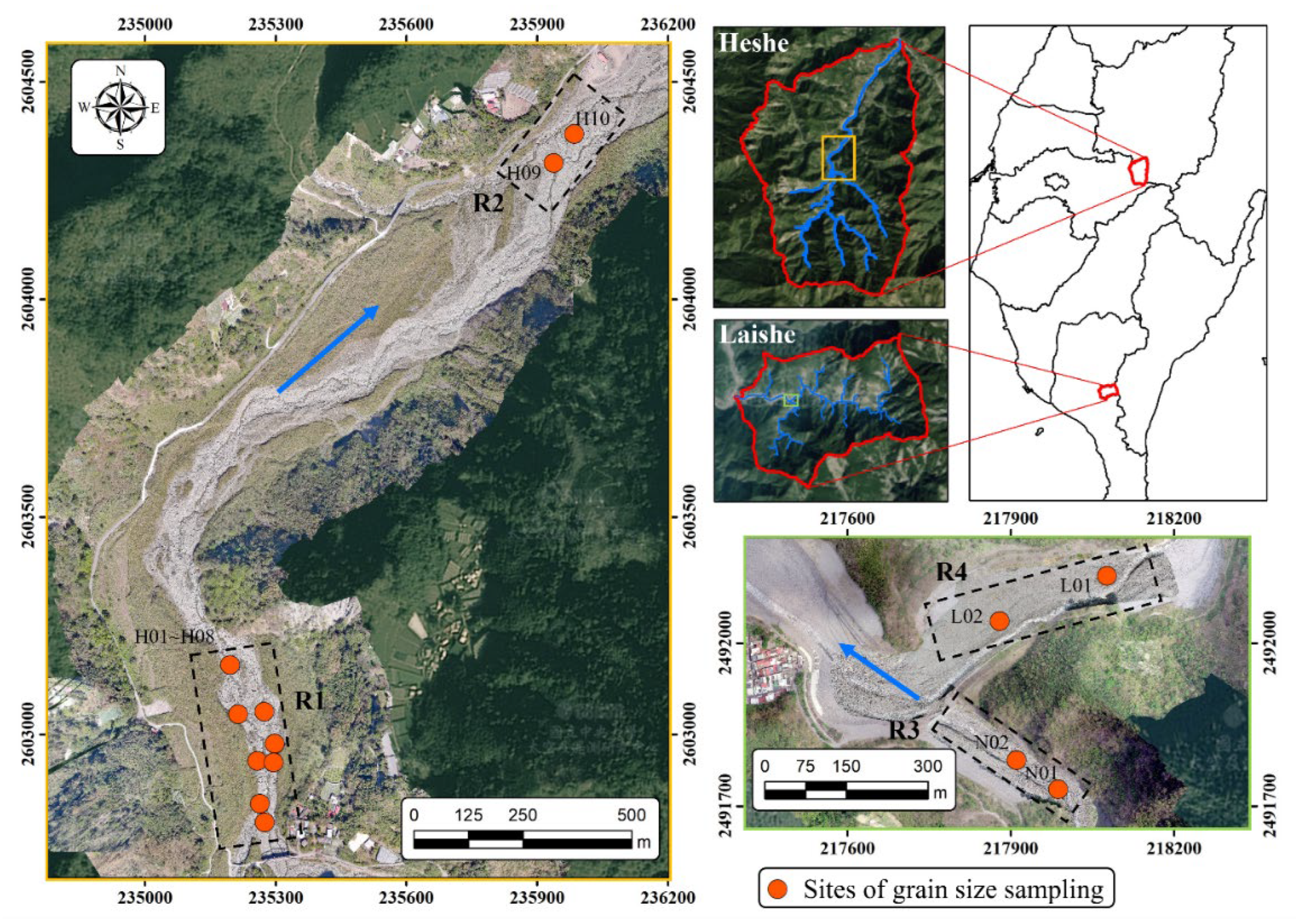
Figure 2.
The schematic diagram for evaluating the roughness height.

Figure 3.
Three roughness distributions by three kernel radii and their comparison with grain size distribution by manual sampling.
Figure 3.
Three roughness distributions by three kernel radii and their comparison with grain size distribution by manual sampling.
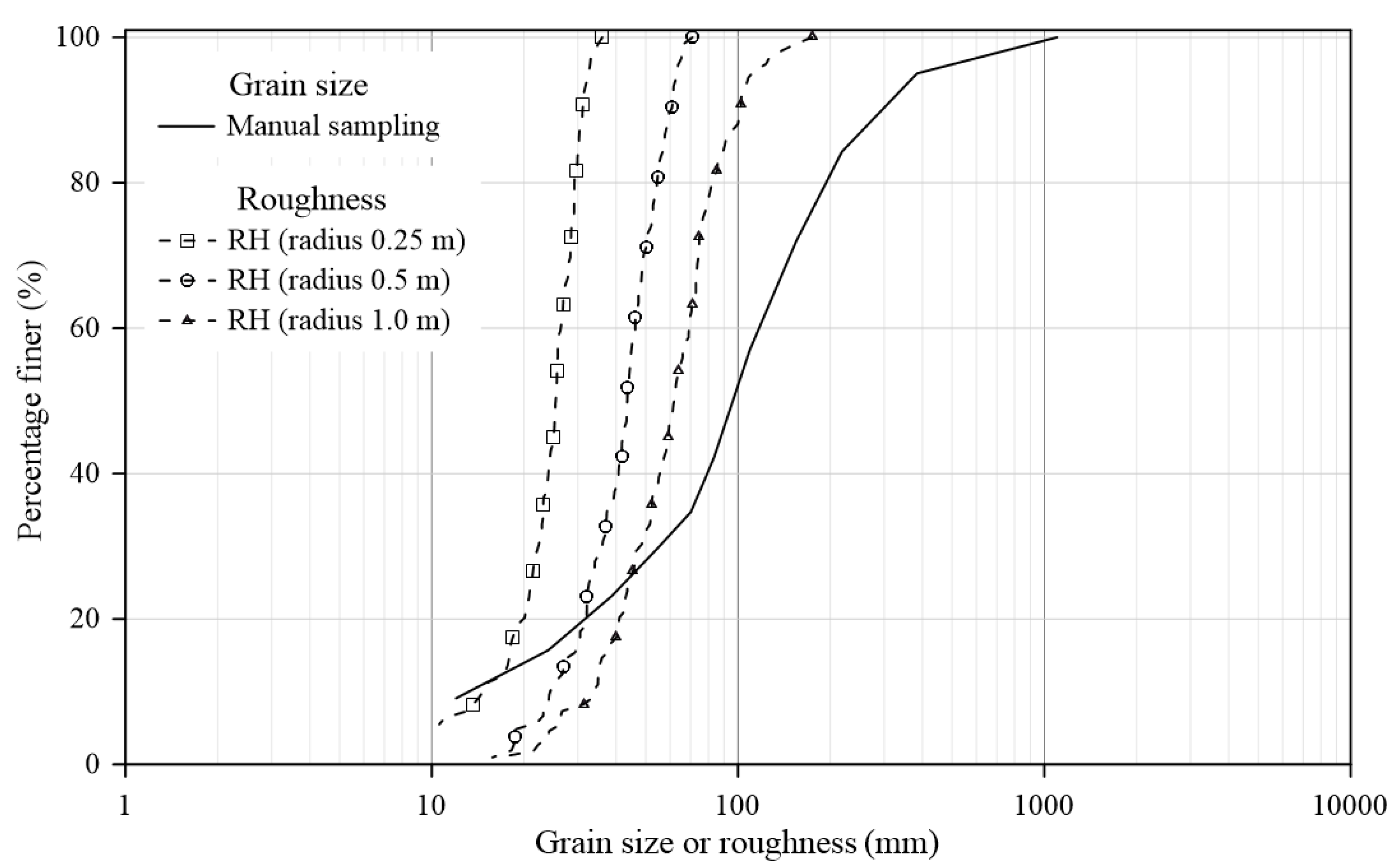
Figure 4.
The research flow chart for present study.
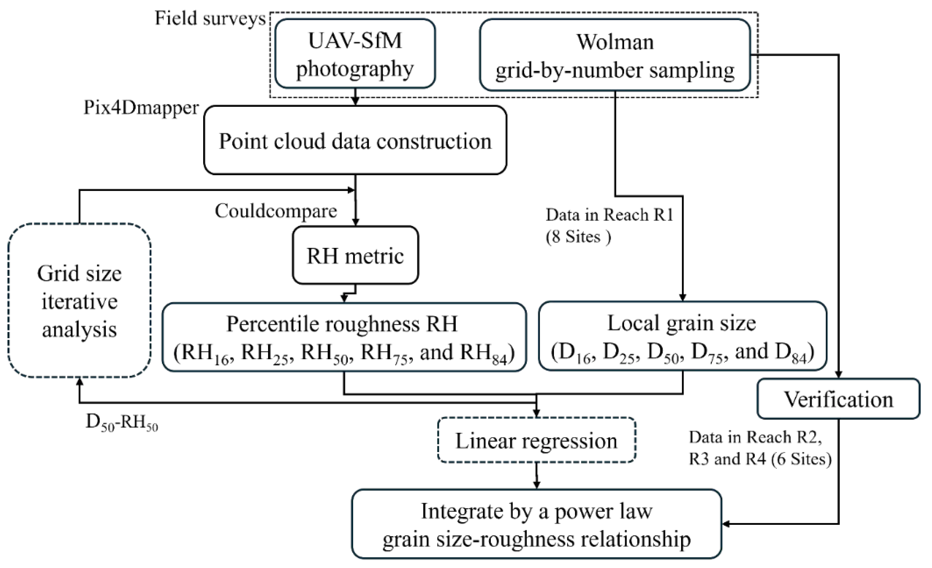
Figure 5.
The variation of R2 in the D50-RH50 relation for RH obtained by eight kernel radii.
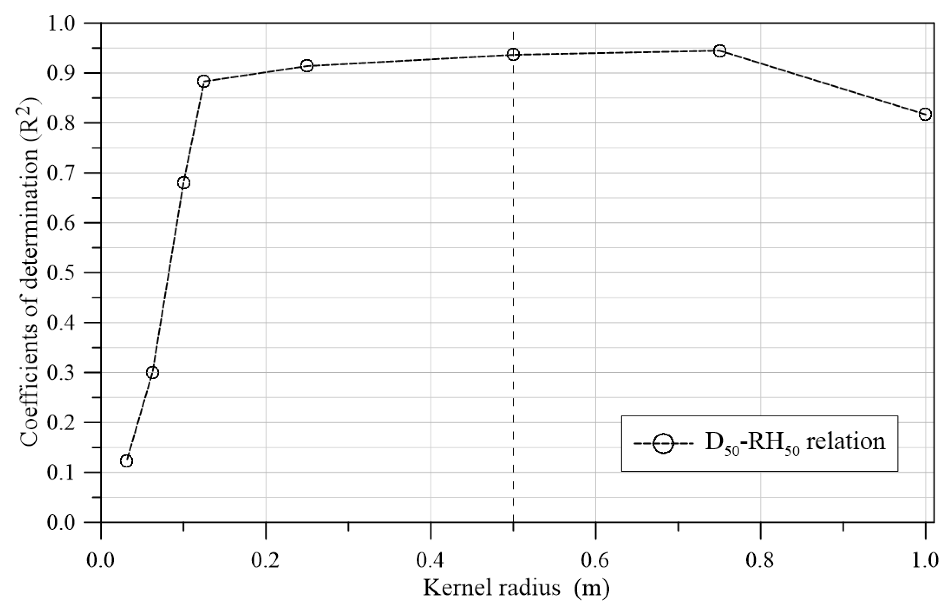
Figure 6.
The relations of Di and RHi and their linear fitting lines.
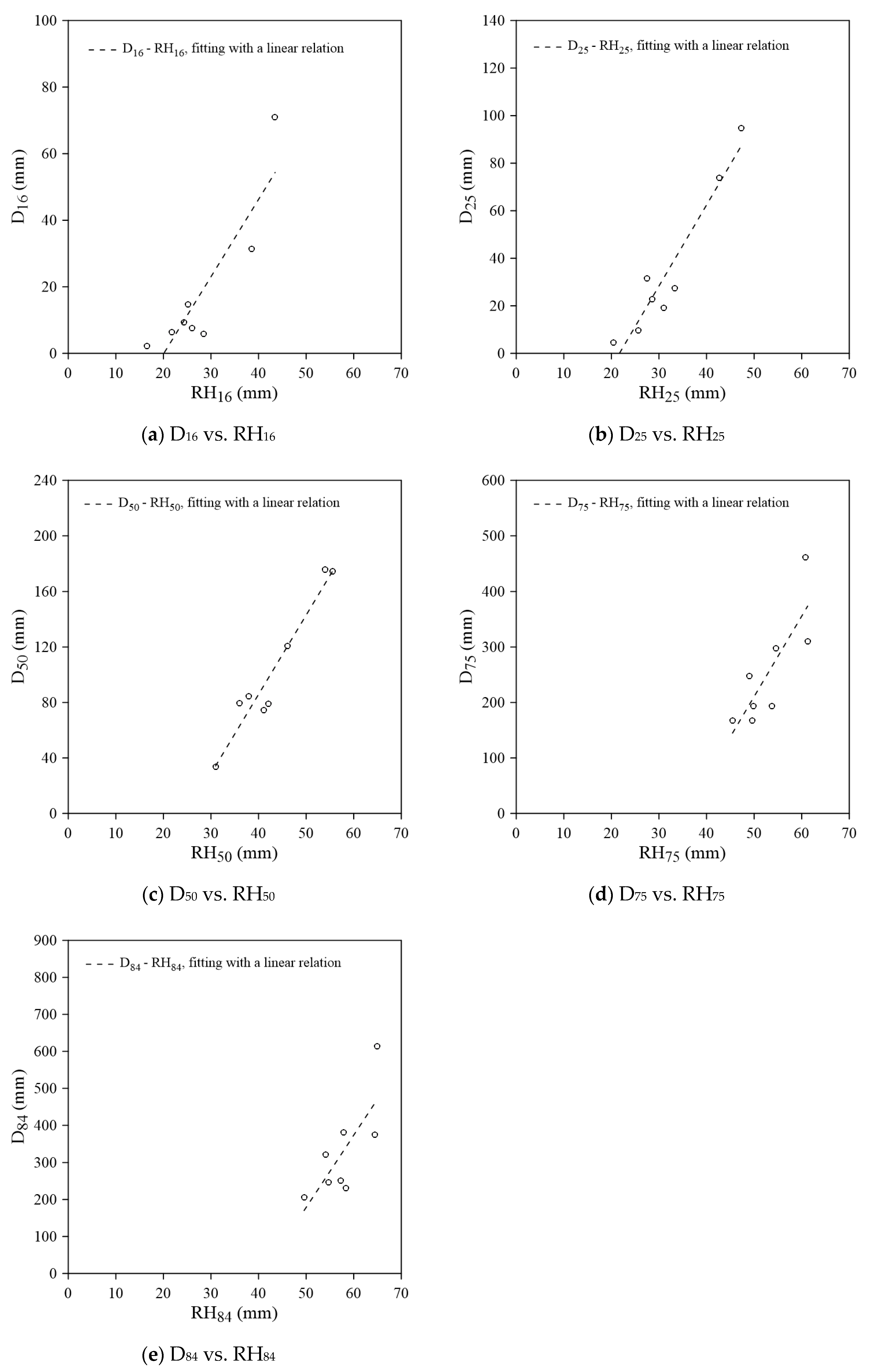
Figure 7.
The variation of the regression slopes (), and intercepts () with respect to different Di-RHi.
Figure 7.
The variation of the regression slopes (), and intercepts () with respect to different Di-RHi.
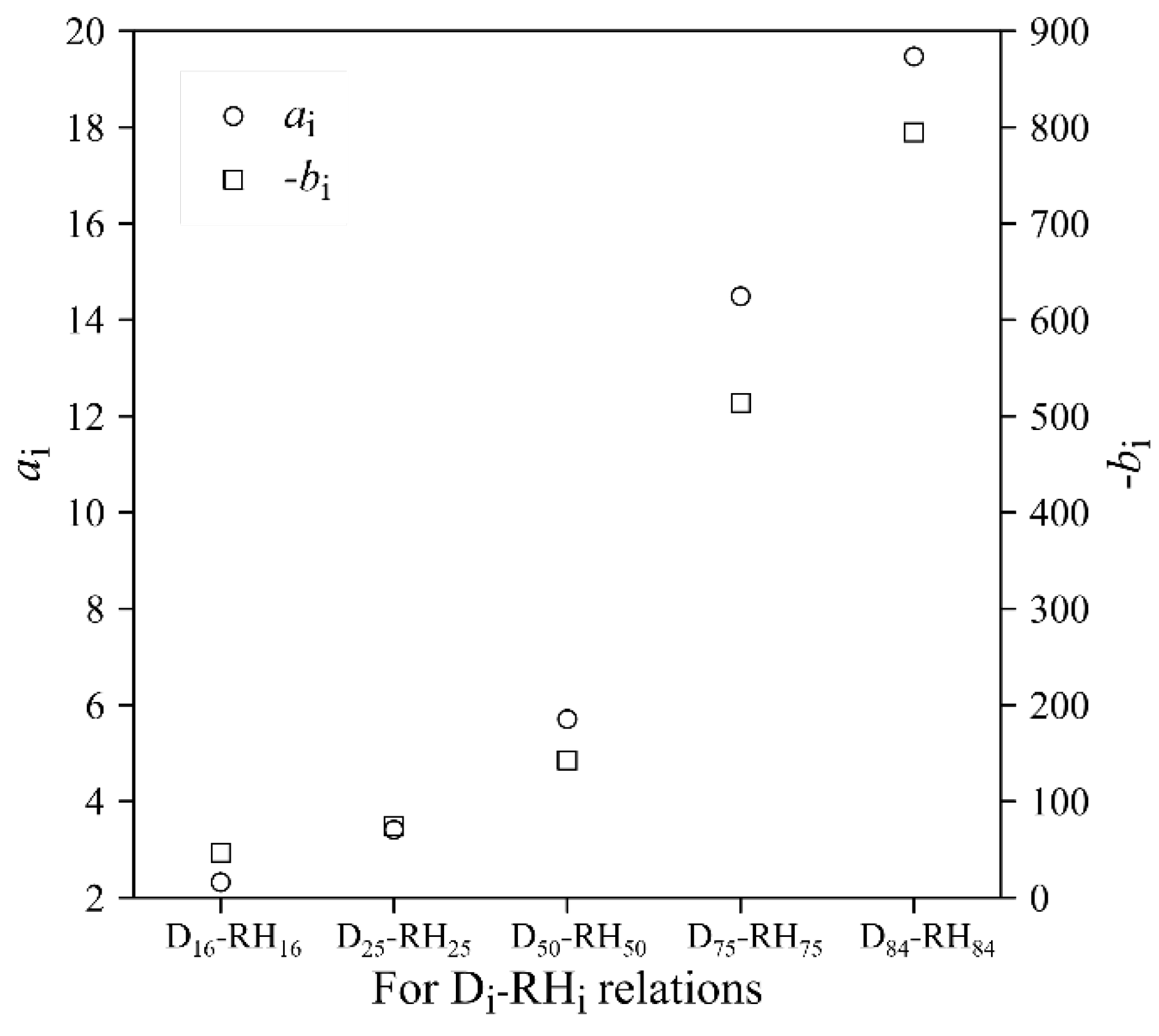
Figure 8.
Integrating the grain size-roughness relations by a power law relation.
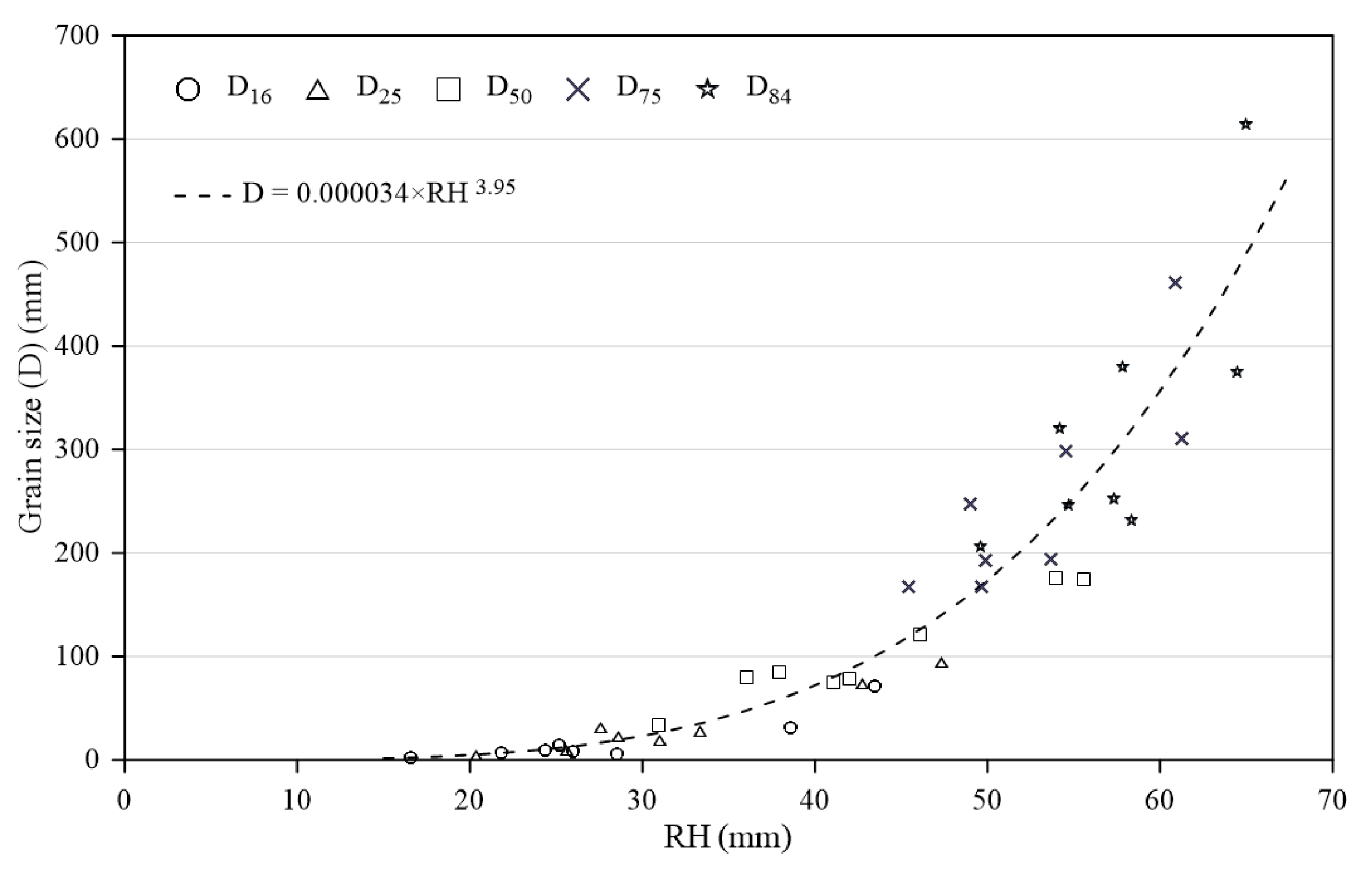
Figure 9.
The comparisons of grain size distribution estimated from the integrated grain size-roughness relation with those by manual sampling for six different sites.
Figure 9.
The comparisons of grain size distribution estimated from the integrated grain size-roughness relation with those by manual sampling for six different sites.
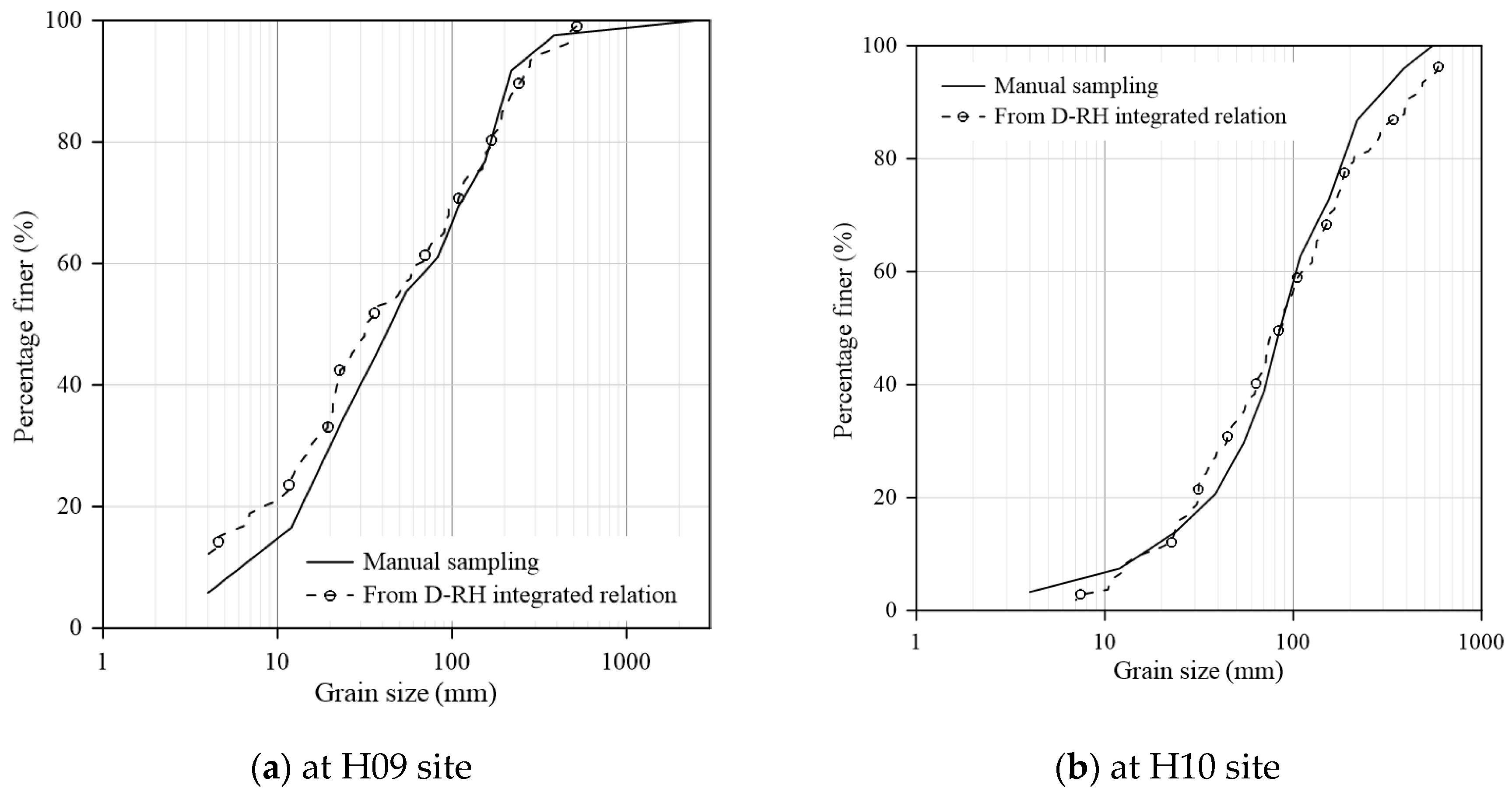
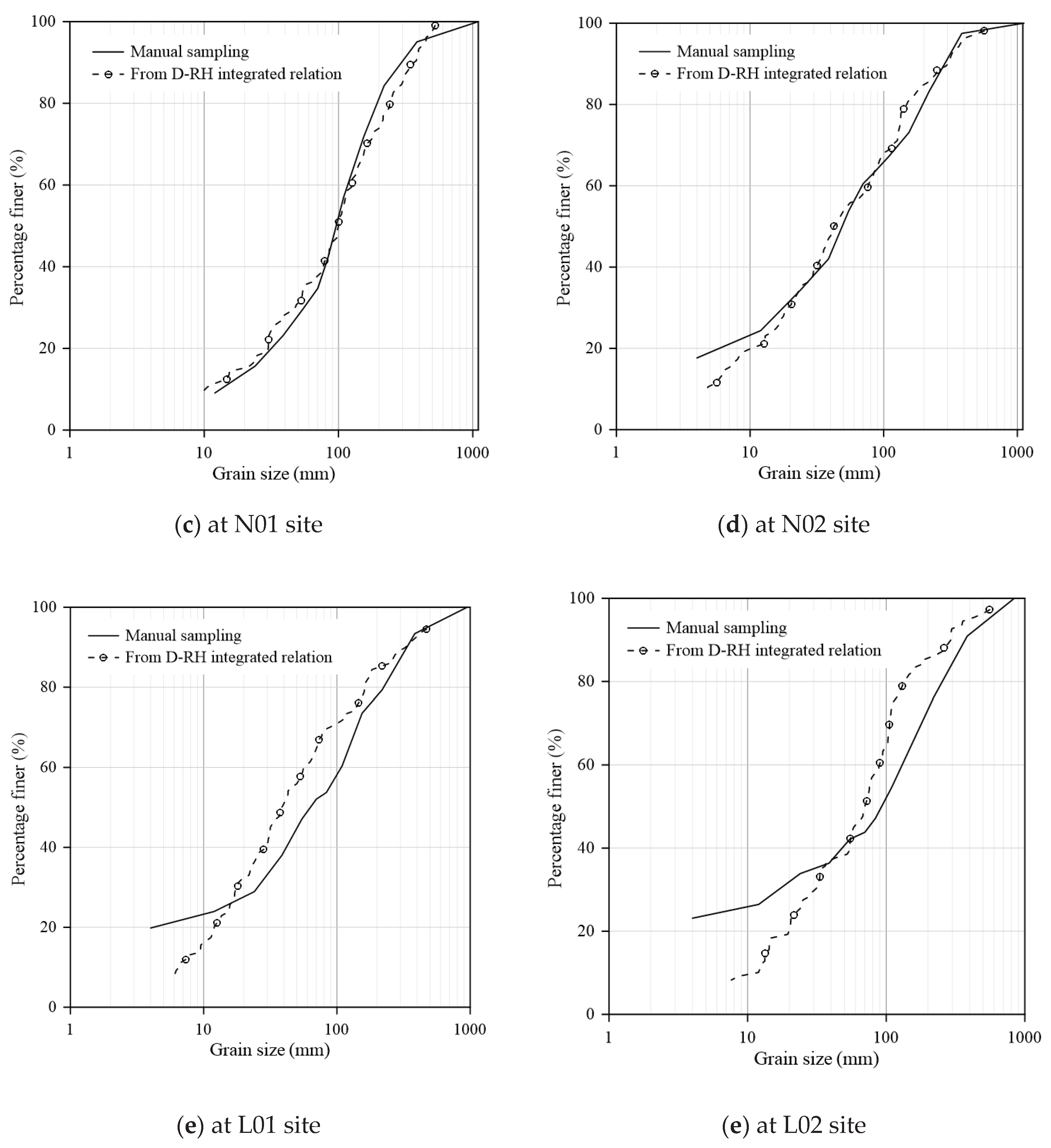
Figure 10.
The variation of R2 in Di-RHi with different dimensionless grid sizes.
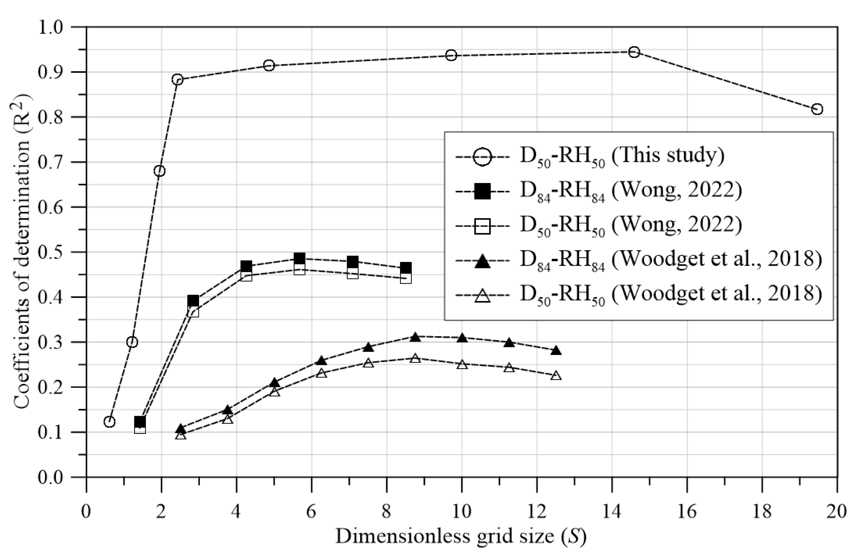
Figure 11.
Comparison of the grain size-roughness relations from the previous study.
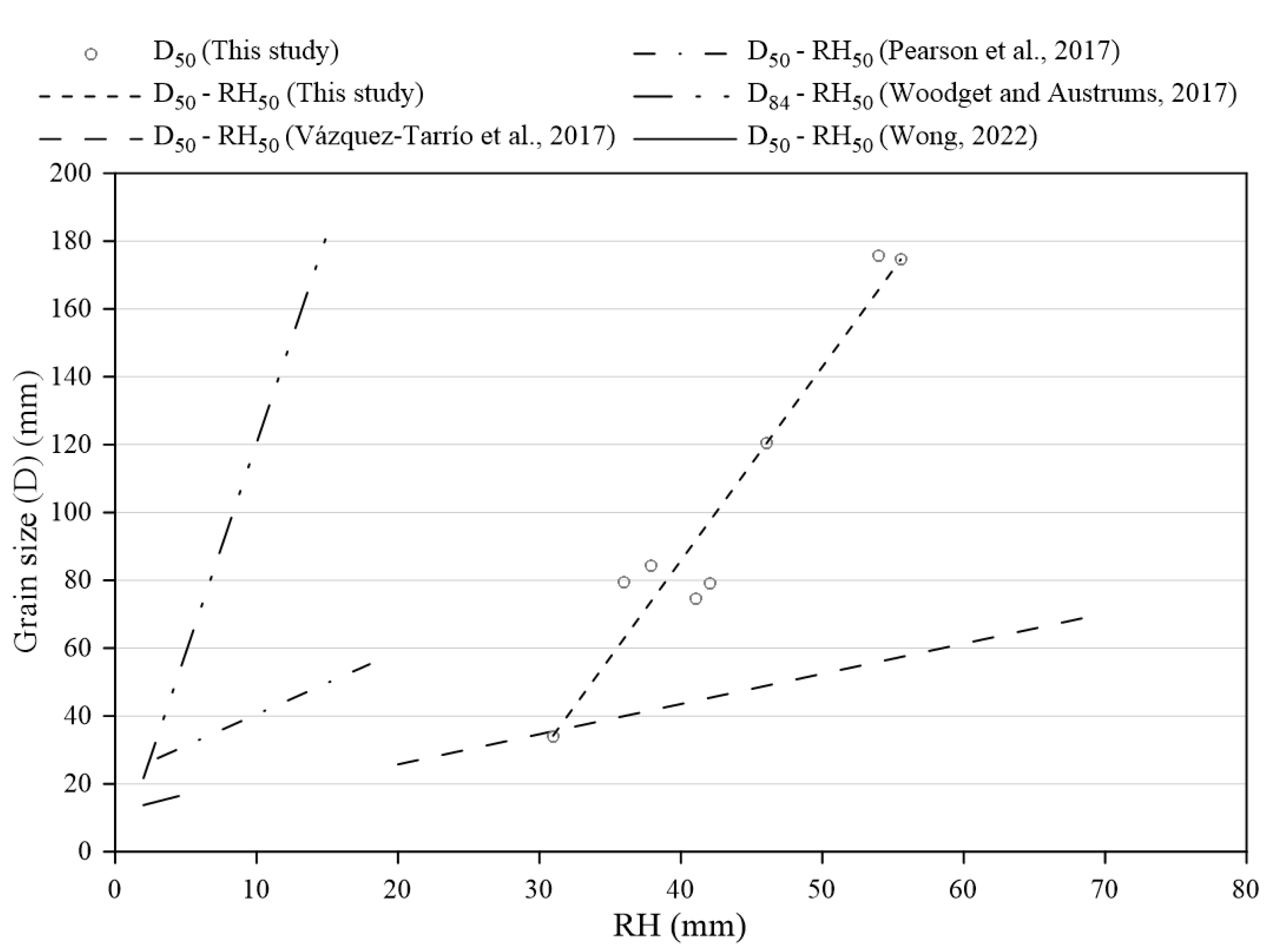
Table 1.
Summary of grain size-roughness relations obtained by previous researchers (modified from [16]).
Table 1.
Summary of grain size-roughness relations obtained by previous researchers (modified from [16]).
| Researchers | Sediment Description (Grain Size Range) |
Grain Size Sampling | Data | Roughness Metric* (Grid Size) | Grain Size-Roughness Relation (in Meters) | R2 |
|---|---|---|---|---|---|---|
| Heritage and Milan (2009) [15] | Gravel-bed river with discs dominating (10~140mm) | Pebble counts | TLS | 2σ (0.05m) | D50 = 0.73(2σ) + 0.037 | 0.37 |
| Hodge et al. (2009) [20] | Tabular form and rounded edges (18~63mm) | Pebble counts | TLS | σd (1.0m) | D50 = 1.42σd + 0.009 | 0.65 |
| Brasington et al. (2012) [14] | Schistose, cobble-sized grains (D50 in 30~117 mm) |
Pebble counts | TLS | σd (1-2 m) | D50 = 2.59σd + 0.012 | 0.92 |
| Woodget and Austrums (2017) [19] | Cobbles and boulders (D84 in 10~160 mm) |
Areal sample & Photosieving | SfM | RH (0.4m) | D84 = 12.35RH–0.003 | 0.80 |
| Vázquez-Tarrío et al. (2017) [17] | Well-rounded and subspherical grains (D50 in 30~70 mm) | Pebble counts | SfM | RH (1.0m), 2σ (1.0m) & σd (1.0m) | D16 = 0.73RH +0.0073 | 0.64 |
| D50 = 0.89RH+0.00795 | 0.89 | |||||
| D84 = 0.78RH + 0.019 | 0.83 | |||||
| Pearson et al. (2017) [16] | Oblate (53%), prolate (24%), and sphere (23%) shaped particles. (74~288mm.) | Areal sample | SfM | σ (0.2m)& RH (0.55m) | Poor sorting D50 = –0.29RH + 0.050 |
0.02 |
| Moderately well-sorted D50 = 1.85 RH + 0.022 |
0.69 | |||||
| Wong (2022) [12] | Sands, gravels, and cobbles (D50 in 14.1 mm, D84 in 25.1 mm) |
Photosieving | SfM | σ (0.03m) RH (0.08m) |
D50 = 1.07RH + 0.0116 | 0.46 |
| D84= 3.87RH + 0.0137 | 0.48 |
*σ: Standard deviation, σd: Detrended standard deviation, RH: Roughness height.
Table 2.
Seven field surveys in the studied reaches for UAV photography and grain size samplings.
| Set | Date | Reach | Point Cloud Density (pts/m3) |
GSD (mm/px) |
Georeferencing Errors (cm) |
Grain Size Sampling Sites |
|---|---|---|---|---|---|---|
| 1 | 2021/12/15 | R1 | 15564.2 | 5.8 | 0.8 | H01 |
| 2 | 2022/10/24 | R1 | 8502.6 | 7.2 | 1.8 | H02, H03, H04, & H05 |
| 3 | 2023/01/05 | R2 | 22833.7 | 4.7 | 2.1 | H09 |
| 4 | 2023/07/06 | R1 | 8761.0 | 7.2 | 2.0 | H06, H7, &H 08 |
| 5 | 2023/11/24 | R3 | 13583.9 | 6.3 | 3.2 | N01 & N02 |
| 6 | 2024/01/18 | R4 | 15393.9 | 6.5 | 2.4 | L01 & L02 |
| 7 | 2024/02/21 | R2 | 10688.3 | 7.1 | 1.6 | H10 |
Table 3.
The linear regression relations of the Di-RHi and their coefficients of determination (R2), slope (), and intercept ().
Table 3.
The linear regression relations of the Di-RHi and their coefficients of determination (R2), slope (), and intercept ().
| Di-RHi | R2 | ||
| D16-RH16 | 0.79 | 2.32 | -46.67 |
| D25-RH25 | 0.92 | 3.41 | -73.90 |
| D50-RH50 | 0.94 | 5.71 | -142.58 |
| D75-RH75 | 0.67 | 14.49 | -513.92 |
| D84-RH84 | 0.57 | 19.47 | -794.82 |
Table 4.
The absolute bias of local grain sizes estimated from the integrated grain size-roughness relation with those from manual samplings in 6 sites (unit: %).
Table 4.
The absolute bias of local grain sizes estimated from the integrated grain size-roughness relation with those from manual samplings in 6 sites (unit: %).
| Sites | R2 Reach | R3 Reach | R4 Reach | Average (%) |
||||
|---|---|---|---|---|---|---|---|---|
| Di | H09 | H10 | N01 | N02 | L01 | L02 | ||
| D16 | 42.9 | 3.5 | 3.2 | 113.3 | 229.1 | 418.9 | 136.3 | |
| D25 | 27.9 | 23.0 | 21.5 | 28.3 | 8.7 | 186.3 | 42.5 | |
| D50 | 27.5 | 2.2 | 3.4 | 12.1 | 38.3 | 24.1 | 15.8 | |
| D75 | 0.7 | 8.9 | 33.7 | 20.2 | 17.8 | 46.9 | 20.0 | |
| D84 | 4.4 | 40.6 | 31.0 | 17.5 | 33.5 | 40.9 | 24.2 | |
| Average | 20.7 | 15.6 | 18.6 | 38.3 | 65.5 | 143.4 | -- | |
Disclaimer/Publisher’s Note: The statements, opinions and data contained in all publications are solely those of the individual author(s) and contributor(s) and not of MDPI and/or the editor(s). MDPI and/or the editor(s) disclaim responsibility for any injury to people or property resulting from any ideas, methods, instructions or products referred to in the content. |
© 2025 by the authors. Licensee MDPI, Basel, Switzerland. This article is an open access article distributed under the terms and conditions of the Creative Commons Attribution (CC BY) license (http://creativecommons.org/licenses/by/4.0/).
Copyright: This open access article is published under a Creative Commons CC BY 4.0 license, which permit the free download, distribution, and reuse, provided that the author and preprint are cited in any reuse.


