Submitted:
14 November 2025
Posted:
14 November 2025
You are already at the latest version
Abstract
Trust in machine learning models is critical for deployment by users, especially for high-risk tasks such as healthcare. Model trust involves more than just performance metrics such as accuracy, precision, or recall, it includes user readiness to let a model make decisions. Trust is commonly associated with model prediction stability under variations to training data, noise, parameters, explanations, etc. This paper expands on former model trust concepts with a proposed Model Sureness measure. Model Sureness in this work quantifies stability of model accuracy under variations to the training data for any model by a bidirectional active learning with Visual Knowledge Discovery method. This method iteratively retrains a model on varied training data until a user-defined criterion is met, e.g., 95% test data accuracy. This finds a smaller sufficient training data set for a model to meet the criterion. Then Model Sureness is the ratio of the number of unnecessary cases to all cases in training data. The grater ratio indicates high model sureness in accordance with this measure. Conducted case studies on three common benchmark datasets from biology, medicine, and handwriting recognition show well-preserved model accuracy and high sureness of the respective models. Specifically, removal of unnecessary cases was from 20% to 80% and on average about 50% of training data.
Keywords:
machine learning
; performance metric
; active learning
; visual knowledge discovery
; data reduction
; model sureness
1. Introduction
1.1. Motivation
Trust in machine learning (ML) models by domain experts and users is critical for deployment of models by them [1,2,3,4,5,6], especially for high-risk scenarios such as healthcare or automotive systems [2]. Trust involves more than just performance metrics such as accuracy, precision, or recall — it includes the user’s confidence in a model’s accuracy, personal comfort with understanding it, and willingness to let a model make decisions [3,4]. Trust is commonly associated with stability in the model’s form, i.e. pattern, and predictive accuracy under multiple variations.
These variations include changes to training data, types of noise in the data, learning algorithm (hyper-)parameters, model explanations, and many others. Several concepts of ML model trust have been proposed. This paper expands on them by introducing a Model Sureness (MS) measure which supports several known dimensions in trustworthiness frameworks as described in this paper.
Specifically, the Model Sureness measure studied in this work quantifies the impact of training dataset variations on the stability of model accuracy for a chosen algorithm. For instance, consider an algorithm that can train high-accuracy models even if trained on significantly varied training data examples. These models are referred to as models of high training data Model Sureness. This is considered a prerequisite for a model to be regarded as highly trustworthy [5]. Model Sureness measures of variations beyond training data are beyond the scope of this study. However, the approach used here would only change in the criterion of model success.
It is also possible that the results of the Model Sureness analysis may show that the model, and its accuracy, are extremely sensitive to variations to the training data used. This does not only put in question the trust of the model but also trust in the training data. It may require changing both the training data and the set of features used. Changing data features is also beyond the scope of this study. While Model Sureness measures can help to guide such changes by providing statistics of accuracy, or on any user-chosen threshold metric, and identifying the cases that are significantly impactful to model variability.
We quantify Model Sureness as a measure that is evaluated by using two distinct but complimentary approaches: (1) computational Bidirectional Active Learning (BAL) and (2) interactive Visual Knowledge Discovery (VKD) approaches as presented in this work. For instance, if a much smaller subset of training data can be used to train a model that yields the same properties as the one trained on the full dataset, then this model would be considered to have high Model Sureness. Moreover, the Model Sureness method is looking for the smallest viable training data subset from which to train a model with the same properties.
It is important to consider when analyzing a model for trust that only the known dataset is available, which is likely only some of all possible data. Moreover, the known minimum and maximum values of each attribute may not be its true value given all data. Therefore, uncertainty is present, which is another motivation for developing the Model Sureness approach.
For training data Model Sureness, if removing many cases from training data still allows us to train a model with a similarly high accuracy, then the Model Sureness of this model is high. Figure 1a illustrates an example of a high sureness model and Figure 1b presents an example of a low sureness model. Figure 1 also shows a high influence of the border area on Model Sureness. In Figure 1a 90% of all 20 cases for 18 correct cases were correctly classified, with two cases being misclassified. Moreover, using the 10 cases that are only outside of the oval as training data yields 100% accuracy with no misclassified cases. Using 10 cases that are inside the oval as training data leads to 80% accuracy with two misclassified cases.
In contrast, removing cases in Figure 1b similarly impacts the accuracy much more significantly. The accuracy of classification with all eighty cases (forty red and forty blue) is 90% with eight cases misclassified (four red and four blue). The accuracy with using the cases outside of the oval is 100% without misclassified cases. The accuracy with using the cases inside the oval is 50% with the same eight errors (four red and four blue out of the sixteen total cases inside the oval.
The average accuracy of two subsets from Figure 1a is 90%, this is the same for all data. In contrast, for two subsets for Figure 1b it is only 75% vs. 90% for all data. For Figure 1 we found two subsets with 50% of cases and accuracy no less than 80%, but for Figure 1b we found only one such subset. These simple examples show that to represent Model Sureness it is not sufficient to find a single significantly smaller subset, but we need to also explore how many datasets exist by conducting multiple experiments. Later we define the Model Sureness measure formally and numerically.
It is well known that noise in data obscures patterns and degrades model accuracy. By introducing the Model Sureness measure, we aim to discover models with a stable accuracy despite any noise in the data. Discovery of models with other stable properties besides accuracy is beyond the scope of this work.
The proposed approach trains models sequentially where the next model is trained with updated training data by either adding or removing more cases until a model yields accuracy on the test data that meets a user-specified threshold. This process can also help identify the smallest subsets of training data required for reliable model performance. However, the order in which cases are added or removed from the training dataset can significantly impact resultant models. Exhaustively testing all possible case combinations would be combinatorially infeasible. To decrease computations required and preserve class balance we use stratified sampling repeatedly in exploration of plausible scenarios. As a result, the process is stochastic through experimental repetitions.
Noisy cases in training data are often associated with non-representative patterns that obscure meaningful structure. In our case studies, the process eliminated from 20% up to 80% of such noisy or redundant cases with 50% of cases being eliminated on average.
The benefit of this approach is not only in reducing data volume, but in identifying which cases are truly representative for building the model. This method is conceptually aligned with [6], which identified worst-case training instances via a Visual Knowledge Discovery process.
Discovering truly representative data by visual means often enhances pure analytical approaches [7,8,9]. While cutting down the number of training cases is especially relevant for large datasets, such as the MNIST handwritten digit dataset [11] that contains 60,000 training cases in a 784-D feature space. Case study 5.3 examines this scenario showing that models can be discovered with comparable accuracy extracted from a subset of only 9,600 cases instead of all 60,000 cases resulting in substantial computational benefits.
1.2. Challenges and Opportunities
Reducing the number of training cases may not always be successful. A significant decrease in accuracy after removing some training cases implies that these cases are strongly representative of its class or play a key role in revealing class patterns.
We can assess impactful cases through visual inspection in a lossless visualization by comparing them to their nearest neighbors that are not similarly impactful. Conversely, if model accuracy remains largely unaffected by the removal or addition of selected cases, those cases are likely not representative of the most representative class structure or even can represent noise.
In general, we can vary any characteristic in the model construction pipelines—such as attributes, parameters, and other design choices—and measure model stability for them as one of the model trust indicators. For instance, this process can identify a stable and relevant subset of data attributes. Moreover, trust in a model depends on the assumptions made during its construction. Unfortunately, users are rarely aware of these assumptions, yet in high-risk domains like healthcare diagnosis, such assumptions require critical scrutiny.
The common ML assumption that the distribution of unseen data will match the training data distribution limits potential deployment in trust-critical applications. This assumption, while potentially reasonable at the population level, fails to account for the case-specific variances and outliers. This is especially important for high-stakes tasks, where the cost of error from a single case can be significant. Crucially, we cannot assume all possible data instances are known or that new outlier cases will not emerge. Research shows that atypical cases behave fundamentally differently and can disproportionately impact model performance compared to typical cases [5]. The proposed model sureness measure helps to test the assumptions of distributional similarity between training and unseen data. Formally, it enables mathematical bounds of the minimum and maximum training data size required to achieve desired model properties like accuracy.
1.3. Summary of the Proposed Approach
The proposed approach is to enrich abilities to analyze and establish trust in ML models. It consists of a model sureness concept to measure the impact of training data variations on model accuracy for a chosen ML algorithm. The measure of model sureness can be produced by (1) computational Bidirectional Active Learning (BAL) processes proposed in this paper or by (2) interactive VKD processes [7].
The BAL approach allows for dataset reduction for many kinds of ML algorithms. One of the examples is the Generalized Iterative Classifiers (GIC) [6,9]. These models use Generalized Decision Trees (GDTs), which allow for non-binary decision levels. Because each GDT level depends on the structure and composition of the training data, reducing the dataset has a cascading effect, simplifying downstream decision nodes and improving the entire model’s interpretability.
Compared to other computational approaches to find smaller datasets, the proposed automatic Bidirectional Active Learning approach has the following beneficial features further detailed later:
(1) BAL can find smaller training datasets for any user-chosen ML algorithm being an algorithm-agnostic wrapper method in contrast with some other methods reviewed later that are algorithm-specific.
(2) BAL is simpler than other methods that use additional processing when searching for smaller training datasets making it more scalable and highly parallelizable.
(3) BAL allows to control the number of cases tested per step decreasing stopping at local minima in contrast with a binary search halving process and a process based on common cross-validation data splits with 10 or 5 folds.
Next, interactive Visual Knowledge Discovery approach provides additional benefits of active involvement of the user who brings domain expertise to find more relevant smaller datasets. In addition, the combination of BAL and VKD creates additional benefits of faster computation for larger datasets by BAL and deeper user expertise by VKD.
Primary novelty. The primary novelty of this paper is in (1) linking studies that search for sufficient smaller training data with trustworthiness of ML models and (2) proposing a numeric measure of model sureness based on the smaller training datasets. It is in contrast with a common motivation of studies for finding smaller training datasets for faster model computation on the smaller data.
Another important novelty is (3) linking the whole area of multiple existing methods that find smaller training datasets with visualization of high-dimensional data and Visual Knowledge Discovery allowing (4) finding these datasets in visualization and (5) solving ML tasks with visual means, which often is impossible for large training datasets. It is beneficial for both lossy visualization methods like Principal Component Analysis (PCA) and t-Distributed Stochastic Neighbor Embedding (t-SNE) as well as lossless methods like Parallel Coordinates (PC) and General Line Coordinates (GLC) [8].
The rest of this paper is organized as follows. Section 2 covers a literature review. Section 3 outlines the methodology. Section 4 is on Algorithmic Topics. Section 5 presents Case Studies on the Fisher Iris [10], Wisconsin Breast Cancer [11], and MNIST Digits [12] datasets. Section 6 is Discussion, Conclusion, and Future Work; with links to developed open-source software implementation. The paper concludes with the cited references.
2. Related Work
2.1. Model Trustworthiness as a Multidimensional Evaluation Framework
Trustworthiness in machine learning encompasses multiple essential dimensions, each being critical to ensure that models behave reliably, ethically, and understandably. Fairness addresses bias and prevention of discrimination against subgroups with widely studied metrics that measure this like demographic parity and equality of opportunity [13,14,15,16,17]. Robustness measures a model’s stability against noise and adversarial inputs and ensuring prediction consistency under perturbations [24]. Confidence and calibration are ensuring that predicted probabilities accurately reflect true likelihoods, leveraging metrics like Expected Calibration Error and Brier score [25,26,27]. Interpretability is understanding model decisions via feature importance rankings and explanations aligned with domain knowledge [28,29,30,31,32,33]. Safety and security ensure models behave reliably under adversarial or edge cases, incorporating fail-safe design principles [34,35]. Lastly, Transparency and accountability measure the understandability and auditability of the system’s design and operation, facilitated by documentation standards and governance frameworks [36,37].
Several quantitative metrics unify these aspects into comprehensive measures of trustworthiness. The FRIES Trust Score combines fairness, robustness, integrity, safety, and explainability into a consolidated metric [19]. Stability assessment quantifies overall prediction sensitivity to noise and other perturbations. Confidence intervals calculated on performance metrics provide statistical assurance regarding model reliability. Correlation of feature importance ranks with trusted domain knowledge assesses interpretability quantitatively.
User behavior and interaction metrics in real-world deployments give additional trust signals complementing technical measures [20,38,39]. The NIST AI Trustworthiness Framework codifies fundamental trust traits such as validity, reliability, safety, security, transparency, privacy, and fairness into authoritative guidelines essential for trustworthy AI systems [21,22].
In summary, trustworthy machine learning requires a multidimensional evaluation framework integrating technical robustness, interpretability, fairness, safety measures, user interaction signals, and transparency mechanisms to build trustable AI models and preserve trust in them.
2.2. Model Sureness as Part of an AI Trustworthiness Framework
The proposed concept of model sureness complements existing categories of the AI trustworthiness frameworks. With model sureness a model’s confidence or certainty is quantified by the smallest training datasets needed to achieve a target high accuracy. Model Sureness is most tightly woven into validity (does it have the required accuracy?), reliability (does it hold with diverse data?), and robustness (does accuracy persist as data becomes sparse or shifts?). All these categories require empirical evidence about performance under different data conditions. Model sureness allows us to inform and complement these categories.
Alternative model sureness measures have been proposed for specific domains such as network security and quantum computations [40,41,42], where they focus on uncertainty or repeatability within limited ML contexts.
How Model Sureness Relates to Trustworthiness Components? Model Sureness supports validity (the model’s required accuracy) and reliability (consistent, repeatable performance) because high accuracy with minimal data provides strong evidence of both. If a model can “prove” its confidence with less data, it may also expose where robustness (resistance to data distribution changes) breaks down or where bias emerges due to sparse training. The proposed Model Sureness measure complements the Model Confidence measures, which provide a statistical Confidence Interval (CI) for individual predictions [43] and conformal prediction [44]. Indirectly, it impacts fairness (small data may amplify bias), transparency (revealing minimum requirements clarifies decision boundaries), and safety (knowing limits of reliable use decreases operational risks).
Model Sureness impacts model interpretability/explainability helping to understand model decisions via identifying a subset of training examples that influence the decision. For example, the minimal subset of training data that provides almost the same accuracy as on the whole training dataset seems to influence the model decisions more than other training examples. Due to much smaller size analysis and visualization of these examples is more feasible. Identifying such training examples is formulated as one of the Machine Learning research gaps by the US National Academies for Safety-Critical Applications [2].
Thus, Model Sureness supports several known dimensions in the trustworthiness frameworks, especially validity and reliability—by revealing how little data are needed for dependable and accurate model behavior.
2.3. Approaches to Find Smaller Datasets
While best-subset selection in high-dimensional data is known to be computationally intractable (NP hard) [45], the review of multiple studies below shows the ability to decrease significantly the size of many datasets by keeping acceptable level of accuracy of prediction. This creates an experimental basis for one of the forms of trustworthy metrics for ML models based on it. It is going beyond computational efficiency and decreasing time for data collection which were a major motivation of several prior studies [45,46].
Our goal is complimentary, focusing on its contribution to model trust. It includes decreasing the amount of data required to be visualized for users to analyze data and model. Thus, our goal has important unique specifics of addressing Visual Knowledge Discovery (VKD) challenges, which differ from pure computational knowledge discovery and model trustworthiness challenges. A small dataset has a fundamental visualization advantage vs. large datasets for human analysis and Visual Knowledge Discovery.
2.3.1. Overview of Computational Approaches
Coreset or instance selection is a common approach for reducing the training set size by selecting a representative subset of the original data [47,48]. Coreset selection uses criteria such as diversity, coverage, and influence. Mostly current coreset methods use heuristic strategies and assumptions due to intractability of the full task. This includes: (1) preserving the consistency of data distribution between subsets and the original ones, (2) minimizing the distance between centers of the selected subset and the original dataset by adding one sample time [49,50,51], (3) bilevel optimization [52], and (4) minimizing the total difference between gradients produced by the subset and the original set for the same neural network [53]. A most updated review of the work in this area is presented in [54].
In a generalized coreset a weighted case can differ from the actual training cases, where the weight of the case can be the number of real training cases it substitutes. For visualization, this repetition of the case can be captured by the wider lines or larger other visual elements that represent it.
The work under the names of Data distillation (DD) and data condensation (DC) [45,46] has a specific aspect – a smaller dataset includes synthetic cases, based on which the trained models yield performance comparable as those trained on the original dataset. While this gives an important advantage for many studies, especially for securing the original data, for exploration of model trustworthiness in this approach has additional challenges – to ensure trust of the model built on the synthetic data. However, this has a fundamental potential benefit for visualization. It opens an opportunity to synthesize cases that will be simple in visualization for human perception and analysis.
Knowledge distillation (KD) or model distillation (MD) comprises training a smaller distilled network on a data set called the transfer set that can differ from the whole training data of the large model [55,56]. When the original training set is unavailable, synthetic or unrelated data can sometimes be the transfer set, with some performance trade-offs. The transfer set often is smaller than the training set used for the large model. Many efficient distillation methods successfully use subsets ranging from 10% to 75% of the original data, balancing resource constraints and performance [57,58,59,60] Thus, transfer sets could be used for the purposes of our study with visualization and trustworthiness.
Below we overview some specific approaches for getting smaller sets. They rely on iteratively or algorithmically measuring performance as data are removed or subsets are intelligently selected, validating against the fixed target accuracy (e.g., 95%). The defined “smallest subset” varies depending on the dataset, model, and required accuracy, but the measurement techniques are generally empirical (progressively reduce data, measure of effect) or algorithmic (optimize subset selection with validation feedback [61]).
Empirical Subsetting and Evaluation studies like [62] divide the training dataset into progressively smaller fractions (e.g. 1/2, 1/4, 1/8, 1/16, etc.). Models are trained on each subset and evaluated on test data. Stochastic and Algorithmic Selection methods use stochastic search or optimization to iteratively select candidate subsets and train/evaluate models on them by testing against a threshold [54]. Wrapper and Heuristic Methods will repeatedly select and evaluate different combinations of training examples, guided by heuristics (such as diversity, margin-based active learning, or representativeness), until the validation or generalization error stays below a chosen threshold [66]. Theoretical constraints and Information Criteria used include feature selection criteria like the Gini index, information entropy, theoretical constraints include assumption about the model type, covariance matrixes and others [67] to determine the minimal training subset that still supports the user’s desired prediction accuracy.
Some other algorithms and strategies designed to identify the most informative or valuable training data for achieving high accuracy in machine learning are listed below. These approaches focus on data selection, active sampling, or automatically ranking the value of training samples. The choice among them depends on the problem domain, data scale, and associated training costs.
Active Learning Algorithms start from a smaller dataset and try to identify the most promising expansion of the dataset for labeling and training [68]. The iterative techniques for this include uncertainty sampling, query-by-committee, margin sampling and others. Influence Functions assess impact of individual training cases on the model’s predictions, allowing identification of data cases that most strongly affect accuracy [69].
Gradient-Based Sample Selection uses the gradients or loss changes with respect to network weights—e.g., selecting cases that induce the largest gradient updates, or that are most representative of the expected “learning signal.” [70]. Submodular Optimization uses mathematical frameworks of submodular set functions to select a highly informative and diverse set of training cases for model training [71,72,73]. Ensemble and Tree-Based Algorithms such as Random Forest and Gradient Boosted Trees naturally use importance of features and instances, helping to rank or select the most informative data cases for training [74]. Learning Vector Quantization (LVQ) selects representative “codebook” cases to summarize and train on the most informative cases, leading to memory-efficient models and robust performance [75].
Similarity-based algorithms like k-Nearest Neighbors (k-NN) are valuable for data subset optimization because they directly leverage the concept of instance similarity to inform which samples may be most relevant or redundant within a dataset. Their roles in this context include identifying redundant points or representative/prototype points for a condensed subset selection.
A study [76] explores the notion of trustworthiness in reduced datasets within data distillation approach with focus of outliers and detection of data out of the distribution producing a method called Trustworthy Dataset Distillation (TrustDD).
2.3.2. Examples of Sufficient Smaller Training Datasets in Literature
Several studies explored the challenge of determining the smallest subset of training data needed to achieve an acceptable performance. Below we provide some examples.
Experiments in [62] on standard benchmarks (MNIST, CIFAR-10, CIFAR-100) demonstrate that it is possible to reach accuracy comparable to full training with much smaller subsets. The study finds that computing expenses can be reduced dramatically by up to 90%, with minimal drop in accuracy, but notes that further testing on larger datasets is required for generalizability.
In [63] an active learning algorithm outperformed other subset selection methods. For CIFAR-10, an active learning margin-based selection keeps the full test accuracy (within 0.5%) with only 50% of the data, and for CIFAR-100, accuracy remains close to full-data performance with 80% of the data.
The experiment in [64] shows a decrease of the data of 80% - 91% for the Wisconsin Breast Cancer 30-D data and a part of MNIST data with a minor drop of accuracy. We conducted experiments with Wisconsin Breast Cancer 9-D data reported in section 5.2.
In [65] a decrease of the data size by about two times is reported for the compound datasets in the empirical machine learning study with a comparable accuracy.
The most significant drop in the number of training cases is reported recently in [54] for the SpIS (Stochastic Perturbation Instance Selection) algorithm. It produced an average training dataset reduction to 3.10% of the original training dataset size. This represents a 96.9% reduction in data volume while maintaining performance. It is obtained with 43 diverse classification datasets, 6 different wrapper algorithms, and 5-fold cross validation methodology. Performance was statistically equivalent to the full training data set at a 5% level of significance.
The algorithm is designed as a wrapper method, meaning that it can work with any machine learning algorithm and corresponding performance metric, making it applicable across different domains and use cases. Parameters related to randomness such as the distribution and magnitude of perturbations are chosen by the Simultaneous Perturbation Stochastic Approximation framework.
2.3.3. Interactive Visual Approaches for Finding Smaller Training Sets
A Computational Interactive Visual Learning (CIVL) process that is conducted with a human-in-the-loop [7] is applicable for finding the smaller training datasets. Below we outline that approach and illustrate it with an example. A Divide and Classify process splits training cases into simple and complex, classifying these separately by computational analysis and data visualization using lossless visualization spaces of Parallel Coordinates or other General Line Coordinates.
Simple cases are those that are in pure areas of the visualization space; these are areas where only cases of a single class are present. The complex cases are cases in the overlap areas where cases of several classes are present. Since these pure training cases are already classified with 100% accuracy, we can test if the accuracy of the test cases in the pure areas found in the training data area is acceptable. If this is confirmed, then we can search for a subset of training cases from those pure areas that are sufficient to keep a high accuracy of classification. The cases in the overlap areas can be kept in the training data without removing any of them. In this way we can get a smaller training dataset if the number of overlap cases is a small fraction of all training cases. Figure 2 illustrates this.
The example in Figure 2a shows a few sufficient training cases for linear threshold classifiers for Iris data [7]. These data have two pure areas: (1) area above the upper orange line and (2) the area below the lower orange line. Case b above the upper orange line is the lowest case of the upper pure area. Respectively, case a is the top case of the bottom pure area. Cases c and d that are next to them are the bottom and top cases of the overlap area. Cases a and b are sufficient to classify all pure training cases. If they also classify correctly test cases in those areas, then they are sufficient to classify them too.
Figure 2b shows all data of two Iris classes in Parallel Coordinates with the edges of pure areas identified. A user can interactively identify smaller sufficient training data by using this visualization. For the pure area above the upper black line, only the case that is represented by that black line is sufficient. For the pure area below the lower black line, only the case that is represented by that black line is similarly sufficient. To find an optimal accuracy threshold several points in the overlap area between the black lines are needed to find a sufficient smaller training dataset.
2.3.4. Comparison of Bidirectional Active Learning with Other Methods
Below we compare the approach presented in this work called Bidirectional Active Learning (BAL) with those described above to find smaller datasets.
User-chosen ML algorithms. BAL can find smaller datasets for any user-chosen ML algorithm. In contrast, gradient algorithms [53,54] or algorithm-specific methods are limited to finding smaller datasets that are only applicable to training just by that ML algorithm.
Scalability. BAL differs from algorithms that generate synthetic data [45,46], rank data points with other models [75], or use other additional processing when searching for smaller datasets. BAL does not involve such additional processing, which makes it more scalable for larger datasets Such uniformity of processing makes it highly parallelizable and more scalable over the splits, cases tested per step, and iterations. For faster and more scalable computation BAL can use resources in parallel.
Robustness. BAL allows to control the number of cases tested per step, making it fine-grained with lower the number of cases per step. It leads to more stable results in multiple runs and decreasing stopping at local minima in contrast with a binary search halving process [62].
Compared to the Cross-Validation (CV) processes [54], the proposed Model Sureness approach can be more robust since it can be more fine-grained. Consider the CV approach using some k-fold CV, say 5-fold, 10-fold, slicing the data to k pieces for study. Each fold in 10-fold of CV contains 10% of training data, and each fold in 5-fold CVS contains 20% of them. in BAL in contrast, we grow or shrink the training dataset to some user-defined m cases. In our study we used much smaller number of cases m in the range of 1%. With such big subsets the CV approach can end up stuck in local minima more often than a fine-grained BAL approach. This makes the proposed BAL approach more robust and able to reveal more accurately highly influential training data examples.
Automation. BAL is automatic in contrast with interactive approaches presented in section 2.3.3. Therefore, it requires less time from the user to find a smaller training dataset for any ML algorithm.
2.4. Emerging Principled Trustworthiness Metrics
The goal of evaluating trust of the model is to give users convincing information to risk deploying the model. It is especially needed for high-stakes applications like medical and financial ones. Users should be convinced by that information. This requires defining principled trustworthiness metrics that we discuss below.
The fundamental challenge of designing trust metrics is to capture multiple aspects of the model trust. Model interpretability is one of them, including feature attribution, i.e., revealing the importance of different features in the black box ML model. If a user accepts feature attribution as faithful, then it can add some trust to the model and desire of the user to use and deploy the model. The same applies to other characteristics of trust, and the more they are provided and accepted by the user the more trust the model has.
Several metrics for feature attributions are analyzed in [77] stating an insufficiency in any of its single categories to accurately measure the faithfulness of feature attribution methods. It is suggested to evaluate them together through cross-comparative analysis to understand their strengths and weaknesses to provide insights until more principled metrics emerge. Foremost, [77] pointed to the lack of explanation for the ground truth information and resulting in the lack of single natural metrics to quantify the faithfulness of the explanations produced by feature attribution methods. They suggest circumventing it by perturbation-based metrics as an approach without using ground truth information. This is a vulnerable approach to getting more principled metrics due to the lack of needed information.
The fundamental principled solution can come from the ground truth information not from avoiding it. A possible source of ground truth information is directly from the end users/domain experts. This human can be in the loop personally or via a model of domain knowledge of that human also called Expert Mental Model (EMM).
A user can respond to provided model trust information/metrics in four distinct ways: (1) full acceptance, (2) full rejection, (3) partial acceptance and/or rejection, and (4) asking to explain the reason in user’s domain terms without machine leaning terms that are “foreign” to the domain. In situations (2)-(4) extra effort is required. In the medical applications in includes translation to terms that are “native” to doctors and patients and provide reasoning in these terms. It is challenging when the domain knowledge model of the domain experts end users is not available explicitly or implicitly, which is beyond training data and the black box model.
Below we discuss the ways this additional domain knowledge can be provided in a realistic fashion. First, it is not a new problem as it was explored for decades in relational machine learning where domain knowledge is recorded in the First Order Logic (FoL) statements [78]. Another way is inspired by the axioms of Shannon information theory. These axioms lead to a specific provable definition of Shannon’s information. Here a user needs to understand and accept these axioms for a specific task. A similar approach can be applied in machine learning model trust studies. It is a more meaningful and scientific way to justify trustworthy approaches than by pure computational metrics without any user involvement.
In the proposed approach to the Model Sureness measure domain experts are asked if they would accept the concept of the Model Sureness expressed in plain English. An example is below. A user is informed that cutting down given training data by 80% still produces a model with almost the same accuracy as the accurate model on all data. We ask domain experts explicitly: “Do you agree that significant decrease in the number of required training data is an extra argument to accept the model as more confident, surer?” If a user accepts this concept as a measure of confidence in the model, then we can say it is a satisfactory approach. It does not need artificial computational metrics, which are not based on the user’s input. If a user rejects the concept of the model sureness articulated in this way, other trust characteristics need to be explored as adequate for the task at hand.
3. Methodology
3.1. Bidirectional Active Learning (BAL) Process
The proposed Model Sureness approach relies on Bidirectional Active Learning (BAL) process of adding or removing data training data. To compute Model Sureness (MS), we iteratively grow or shrink the training data, retraining models each time. This process evaluates the stability of model accuracy under data variations. The central goal is to determine how reliably an ML model maintains accuracy and form of the model as the training data changes.
Unlike standard Active Learning, BAL can operate without querying an oracle or teacher, enabling exploration of data sufficiency when all labels are assumed available. Active Learning (AL) proceeds in a forward direction by querying an “oracle” or teacher to label new data points for building improved models [80]. In active learning Iterative Learning (IL) iteratively expands the training data to optimize model accuracy [80,81,82]. The optimization efficiency criteria vary with implementation and task but usually measure the number of labeled cases required to reach the desired accuracy.
In contrast, BAL assumes the availability of a sufficiently labeled dataset. However, this assumption is increasingly practical due to advances in ML-driven synthetic data generation, reducing reliance on manual annotation while preserving essential model properties like accuracy [83,84]. Since manual data labeling is computationally expensive and labor intensive it would prevent these methods from being fully utilized.
Given the assumption of sufficient labeled data, BAL seeks to identify the smallest subset of training examples needed to still capture the dominant patterns necessary for a ML classifier to learn effectively. Such a reduction of machine learning training dataset size has multiple benefits with a few important ones listed below:
(1) Simplified analysis. We can get 8 times less data as our experiments show. This enables visual explanations of the model prediction to be feasible for a wider set of ML tasks with less occlusion. It includes lossless visualization of similar cases to a new case to be predicted.
(2) Lower computational cost. Finding k nearest neighbors (k-NN) of a given case can be computed approximately eight times faster on the dataset reduced by the same factor. In our experiment with k-NN, a 20% reduction in data size resulted in a 5 times speed-up on benchmark data.
(3) Improved deployment efficiency. Reducing data redundancy conserves memory and compute resources, which is especially important for edge devices like mobile, Internet of Things (IoT), and microcontroller platforms.
BAL can be implemented purely computationally as we reviewed in sections 2.3.1 and 2.3.2 and with visualization of multidimensional data losslessly to analyze these data and machine learning models that are built on them [6,7,8,9] as we reviewed in section 2.3.3. In visualization, occlusion of data cases can obscure dominant patterns. Separating these occluding cases can reveal clearer structures in the remaining data, enabling identification of more precise patterns using interpretable frameworks such as decision rules based on First Order Logic (FoL), instead of relying on simpler approaches like decision trees (DT) or models built only from individual attributes [7]. This two-step process allows one to observe and analyze how patterns and models dynamically change as training data size is increased or decreased.
3.2. Theoretical Analysis: Sureness Measure and VC Dimension
In ML it is known that the amount of data needed to train an accurate prediction model is highly dependent on the data complexity [85]. Thus, measures and bounds of this exist for quantifying this issue such as the Vapnik–Chervonenkis dimension (VC-dim) [86]. VC-dim measures the size of a dataset that a given algorithm can classify correctly. The data size is defined by a positive integer pair (n, m), where n is the space dimension (n-D space), and m is the number of cases/n-D points in the dataset. However, the methods to measure this complexity are mostly theoretical, and not well-defined outside of either very generalized cases or specific scenarios [85,86,87]. Instead, more well-defined bounds exist that have been mathematically proven, particularly for upper bounds [85,88,89].
Applying the VC-dimension to binary classification algorithms finds a threshold value m (case count) for a classifier working in each dimension n to classify/”shatter” any n-D dataset without classification errors [85,86,89]. For example, a linear classifier in 2-D space can classify without any error only three arbitrary 2-D points, thus, here we have a pair of (n, m) = (2, 3) [85,86,90]. In other words, a linear classifier cannot guarantee that with any arbitrary 4 or more 2-D points it will correctly classify all these arbitrary 2-D points. Note that for some, not all, datasets with m > 3 it is possible with a linear classifier.
Therefore, the practical value of the pair (2, 3) is very limited for real world ML tasks because all real datasets contain many more cases than just three with instead hundreds, or thousands of them, with very different mutual relations between them. Thus, by the VC-dim all these variable small and large datasets are within the same risk category of misclassification. However, it is intuitive that these risk categories are not the same for different datasets. Figure 3 shows this where the addition of one data case makes an easy classification task much more difficult. Here a single case requires relearning the model’s discriminant line and deteriorates the classification margin. This drastically lowers the Model Sureness on these data.
The key idea of the VC-dim is to find the capacity of a specific ML algorithm A in terms of a pair <n, m>. It is answering the question: “Will the algorithm A be able to classify a set of m cases (n-D points) for all possible split these m cases to k classes?” For example, if we have only two classes k = 2 then the question is: “Will the algorithm A be able to correctly classify any m cases in n-D space and any possible split of these cases to two classes?” Thus, VC-dim measures the capabilities of the algorithm to classify all possible datasets of a given size (n, m).
Respectively, the key application of the VC-dim is to check if an algorithm for the given number of cases m and classes k will be able to classify any n-D data or not. In most cases VC-dim exaggerates the requirements on the algorithm to be able to classify cases for a given dataset, because it checks any possible split of these cases to classes. However, in practice, many ML algorithms operate under an informal data compactness hypothesis that limits split sets. Under the compactness hypothesis, the cases of a single class are located nearby forming clouds. It is also assumed that these clouds form constellations that are separable by linear or non-linear functions. This is a fundamental idea behind various kernel-based algorithms like SVM.
The difference in our approach from VC-dim is illustrated by the following example. Consider m n-D points (C1, C2, …, Cm,) and 2 classes. There are multiple possible splits of these m cases to two classes, such as: (C1) is split from (C2, C3, …, Cm), or (C2) is split from the rest of the cases (C1, C3, …, Cm), or (C1, C2) are split from the remaining (C3, C4, …, Cm), and so on. VC-dimension deals with combinatorics of all possible splits of m n-D points for a given classifier algorithm. In contrast, our model sureness measure deals with this combinatorics of subsets of a single actual split of m n-D points of the given training data for a given classifier algorithm. Moreover, our model sureness measure deals with splits, where a single n-D can represent cases of two or more classes, which is known to often happen in real training data.
Many modifications of the VC-dim do already exist. They enable rigorous analysis beyond binary classification, such as in multi-class learning, regression, and dynamical systems [90] within a pure computational approach and a general concept of the VC-dim presented above with all possible (n, m) datasets. Some approaches abstract the VC-dim problem to a set-theory perspective [88] or focus on its pure geometric interpretation [89]. The approach in this paper differs from them by dealing with a single training dataset and its subsets, which is not bound by VC-dim defined for all (n, m) datasets.
3.3. Sureness Measure and Visual Knowledge Discovery
We blend computational analysis with visualization [91] to verify and expedite the computational discovery of the minimal machine learning training datasets. This includes support to set up (1) model hypothesis space, (2) a stopping criterion for changing training data, and (3) a model and its interpretation verification. It became possible because the user can visualize the subsets of data where less occlusion is present, allowing for a more truthful understanding of the shape of the data classes. Specifically, the use of lossless visualization on multidimensional data in General Line Coordinates [8,9] allows us to conduct it more completely due to preservation of all multidimensional information in contrast with common dimension reduction methods like PCA, MDS, and t-SNE.
This visualization also allows measuring better model’s accuracy in contrast with a standard “blind” k-fold cross-validation (CV) approach. The CV approach is considered “blind” because it only randomly selects validation cases and can exaggerate the accuracy, because the worst subsets may not ever get selected [6]. We expand on the k-fold CV by running much more times than the usual 10 times (10-fold CV) to mitigate it. Moreover, the process may be seeded by an oracle. This allows for learning a complex metric which is specific to a given classification task.
Relation to well- and ill-posed problems. A problem is well-posed if it satisfies the following conditions (as defined by Hadamard [79]): (1) Existence: A solution exists, (2) Uniqueness: The solution is unique, and (3) Stability: Small changes in input lead to small changes in output). If any of these conditions fail, the problem is considered ill-posed. Typically, ML problems are ill-posed with their solutions (models) violating at least one, or more, of these conditions. The proposed Model Sureness measure is to measure the uniqueness and stability of the ML models relative to variations of training data. This then allows us to judge how well- or ill-posed the problem itself is.
3.4. Model Robustness with Joint Conformal Prediction and Model Sureness Metrics
Conformal Prediction [44] enables models to express not just what they predict, but how sure they are, by outputting prediction sets or intervals that contain the true value with a user-chosen probability (e.g., 95% coverage).
In binary classification, conformal prediction predicts either one or both classes with a user-specified coverage guarantee (e.g., 95% chance the true class is included). This shows where the model is confident (singleton set) or uncertain (both classes). Available training data and attributes or feature set may not be sufficient to classify difficult cases confidently. For instance, a set {‘Virginica’, ‘Versicolor’} is produced instead of ‘Virginica’ only for a specific difficult case. Thus, Conformal Prediction quantifies uncertainty at the individual-case level allowing users to identify less reliable cases for further analysis and enhances user trust for other cases.
The proposed Model Sureness approach seeks the minimal training subset that yields nearly identical accuracy to the model trained on all data. This defines an operational threshold for how much data is truly necessary for the model to be reliable—essentially, a minimal sufficient statistic for empirical accuracy of the model. Thus, both the conformal Prediction and Model Sureness approach are complementary concepts. Since Conformal Prediction identifies the confidence for individual cases and Model Sureness identifies confidence for the whole model. Conformal prediction and the Model Sureness measure have the shared focus of quantifying the uncertainty of the model predictions but by using different means.
Both approaches aim to establish rigorous boundaries for reliable model performance. Conformal Prediction allows us to find subareas of the feature space that are reliable for prediction by the given model. In contrast the Model Sureness approach allows us to find the minimal training data subset that provides nearly identical accuracy to the model trained on all data. Thus, direct benchmarking comparison of these two approaches is not possible because they measure different model trust characteristics. However, they can be combined as we describe below.
Consider a dataset and explore the change in coverage, interval width (for Conformal Prediction), and accuracy (for Model Sureness) as the number of training samples varies. For Conformal Prediction it will be evaluating coverage and size of prediction sets on held-out data after calibration with both full and minimal training sets. However, for Model Sureness, it will be to identify the minimum training data subset size that achieves near-maximum accuracy and then apply Conformal Prediction to measure if the coverage guarantee and efficiency hold similarly. Then analysis is conducted to check if prediction sets remain valid and efficient when using just the minimal Model Sureness subset found, reflecting how well uncertainty is preserved with aggressive data reduction.
Such benchmarking allows us to uncover trade-offs between data efficiency (Model Sureness: how little is needed for accuracy) and reliable actionable confidence (Conformal Prediction: how well does it quantify remaining uncertainty across cases) across varying data and model scenarios. If the prediction sets remain narrow and coverage remains high even as data size shrinks, the model is “sure” with respect to data efficiency, aligning the conformal guarantee with the sureness concept.
Other characteristics of model trust also can be combined with the Model Sureness approach in similar fashion like with conformal prediction. For instance, the methods that generate the importance of the attribute can be evaluated in the full dataset and in the minimal dataset. The difference between them can be analyzed and if it is stable then it adds extra confidence in the model.
4. Algorithmic Topics
4.1. Framework
To study ML Model Sureness, we work with subsets of ML model training data that are modified over many iterations with an ML model rebuilt each iteration to analyze and respond to. The ML model is iteratively retrained, and it is observed whether stable states of accuracy on either growing or shrinking data subsets are reached over many conducted experimental iterations. Algorithms are given step-by-step in section 4.3 showing this overall process for single or multiple splits of training data. The main idea is that as the overall experiment repeats, a minimum and maximum number of cases are averaged, and we check for convergence to an interval bounding the size for a minimal data subset.
If interval convergence is not reached, then it is concluded that the ML algorithm is unstable on the given data for the specified stopping criterion such as some user-selected accuracy threshold This process is simple to implement, scalable to hardware as needed by step-size and iteration count parameters, and can measure different user-selected goal criteria such as model accuracy or noise level.
The process relies on a user selected ML algorithm and some given dataset. The data may have been previously split into train and test subsets such as a 70:30 split being 70% of data to train and 30% to test. Otherwise, the data will be split in the process of testing the Model Sureness. The overall process conducted is demonstrated in Figure 4 flowchart.
The Model Sureness process in Figure 4 has three loops. The first loop runs multiple different data splits ratios to training and test data, like 70%:30%, 75%:25%, 80%:20%. The second loop happens for a given split percentage, like 70%:30%. We produce different training subsets for the same split percentage. For example, the first training data subset includes specific 70% of randomly selected cases, the second training data subset contains another subset that also contains 70% of all cases, and so on. The third loop is building each subset with m cases at a time being added or removed for model training data.
4.2. Definitions
This section defines the main concepts that we work with in this paper.
Definition 1.
Minimal Necessary Training Subset (MNTS): A subset Sm from the given dataset S that is sufficient to train an ML model M to achieve the model accuracy at the level or above the threshold T for a given ML algorithm A, e.g., 95% accuracy.
Thus, Sm is a result of some function F, Sm= F(S, M, A, T) that will be discussed later.
Definition 2.
Maximal Unnecessary Training Subset (MUTS): A subset from dataset S after exclusion of the minimal necessary training subset (MNTS) Sm from S: Su = S\Sm.
Definition 3.
Minimal Magnitude of Training Subset: The number of elements |Sm| is the magnitude the minimal necessary training subset (MNTS) Sm.
Definition 4.
Model Sureness (MS) Measure: The Model Sureness Measure U is the ratio of the number of unnecessary n-D points Su: |Su| = |S| - |Sm| to all points in set S,
U = |Su| / |S|
larger values of U indicate that more unnecessary points can be excluded from the training data to discover a model by algorithm A that satisfies threshold T accuracy. This larger U will also indicate higher potential for user trust in the model.
This definition gives a concrete measure of the reduction in the data redundancy.
Definition 5.
Model Sureness Lower Bound (MSLB): It is a number LB that is not greater than the Model Sureness measure U: 0 < LB ≤ U.
Definition 6.
Tight Model Sureness Lower Bound (TMSLB): It is a Lower bound LBT such that U - LBT ≤ ε, where ε is the allowed difference between U and LBT.
Definition 7.
Model Sureness Upper Bound (MSUB): It is a number LUB that is no less than the Model Sureness measure U: 1 > LUB ≥ U.
Definition 8.
Tight Model Sureness Upper Bound (TMSUB):It is a number LTU such that LTU - U ≤ ε, where ε is an allowed difference of U and LTU.
Definition 9.
Upper Bound Minimal Training Subset: The subset SUB of n-D points from set S that were needed to produce a model with Model Sureness Upper Bound LTU.
Definition 10.
Bounded Noise Reduction (BNR): It is a positive difference Ac(Small) - Ac(Full) > 0, where Ac(Small) is the accuracy of the model on the Small data subset and Ac(Full) is the accuracy of the model on the Full dataset. The idea of this concept is that the Full dataset can contain noisy cases and the removal of them can increase accuracy, which is captured by BNR.
For a practical reason we often search only for an Upper Bound Minimal Training Subset SUB with its Model Sureness Upper Bound LUB. Computationally finding the actual model sureness measure value, or its tight bounds, can lead to an exhaustive search of computing models produced by the algorithm A on multiple subsets of the set S. The number of those model computations NMC and complexity of each model computation CMC depend on the algorithm A, a dataset S, and threshold T for the model accuracy that is set. Respectively, we define these concepts below.
Definition 11.
The number of times that algorithm A computes models {M} on subsets of dataset S is denoted as NMC.
Definition 12.
The complexity of each model computation CMC by an algorithm A on a subset SRi of set S is denoted as CMC(SRi).
Definition 13.
The total complexity of all model computation TMC by an algorithm A on all selected subsets {SRi} of set S is denoted as TMC(S) and it is a sum of all CMC(SRi):
4.3. Algorithms
The algorithms for computing the Model Sureness measure run many times over to analyze different subset selections. In our experiments we used an accuracy threshold of 95%, which is the default in the software developed. This is a user-selected parameter that can be assigned to the user’s task. A user should be familiar with the current accuracy reached for the whole given data and can set the threshold accordingly. Otherwise, pilot experiments should be conducted to identify that level.
For the number of iterations, the default in the software developed is 100, however, this is also adjustable. In our experiments 100 iterations were sufficient to get an accurate Model Sureness measure for different datasets.
The size of the step heavily depends on size of the dataset. In our experiments using about 1% of the dataset was a reasonable starting step that was adjusted by analysis the results. Below we present the algorithms for Model Sureness computation.
- Generalized Data Search (GDS) Algorithm: Is the generalized single-split case that is characterized by the triplet of:
<BDIR, C, IMAX>
Here C is a user-selected criterion that the model is retrained on modified data until achieving. It is represented as a Boolean function such as model accuracy > 0.95.
- Multi-Split Generalized Data Search (MSGDS) Algorithm: Is the generalized multi-split case characterized by the quartet of:
<BDIR, C, IMAX, S, P>
with two additional parameters of S for split percentage (0 < S < 1), where the test subset percentage is the complement 1 – S value, and P is the number of splits to test.
C is a user-selected criterion which the model is built towards achieving. Note, the number of splits trained should be at least up to a number where the resultant Model Sureness ratios barely change with added splits tested.
- Minimal Dataset Search (MDS) Algorithm: It is characterized by a triplet of:
<BDIR, T, IMAX>
Here BDIR is a computation direction indicator bit. BDIR = 0 if the MDS algorithm starts from the full set of n-D points S and excludes some n-D points from S. Bit BDIR = 0 if the MDS algorithm starts from some subset of set S and includes more n-D points from set S. The accuracy threshold T is some numerical percentage value 0 to 1, e.g., 0.95 for 95%. A predefined max number of iterations to produce subsets is denoted as IMAX. This algorithm: (1) reads the triple <BDIR, T, IMAX>, (2) updates and tests the selected training dataset using the respective IMDS, EMDS, and AHSG algorithms, described below.
- Multi-split Minimal Dataset Search (MSMDS) Algorithm: For data that are not split previously to training and test subsets, the user can specify the split number and percentage. Then the MDS algorithm is run a split number of times over percentage sized splits. This gives two additional parameters of S for split percentage (0 < S < 1), where the test subset percentage is the complement 1 – S value, and P is the number of splits to test. Characterized by the quartet of:
<BDIR, T, IMAX, S, P>
- Inclusion Minimal Dataset Search (IMDS) Algorithm: It iteratively includes a fixed percentage of n-D points of the initial dataset S to the learnt subset Si, trains a selected ML classifier A thereon, and evaluates accuracy on all known separate test data Sev. It iterates until all data are added and assessed when reaching threshold T, e.g., 95% accuracy of model.
- Exclusion Minimal Dataset Search (EMDS) Algorithm: In contrast with the above Inclusion Minimal Dataset Search, this algorithm starts on the entire training dataset S and excludes data iteratively to retrain a selected ML algorithm. It also assesses reaching the threshold T.
- Additive Hyperblock Grower (AHG) Algorithm: It iteratively adds data subsets to the training data, builds hyperblocks (hyperrectangles) on the data using the already existing IMHyper algorithm [92], then tests class purity of each hyperblock iteration on the next data subset to be added.
Note, the initial or ending dataset size is determined by the number of minimal cases that can be trained on. This determines the number of initial training cases when adding cases or final training cases when subtracting cases.
Next, Section 4.4 presents scaling considerations and empirical measurements of run time and Section 4.5. details the computational complexity of the approach.
4.4. Computational Complexity
Different ML algorithms have very different computational complexities to run. Therefore, the scaling of Model Sureness computation heavily depends on the selected ML algorithm’s complexity, the number of runs t, and the iteration step m, while other parameters can also impact this computation. In a simplified way, an upper bound of the complexity is t * k * C(A), where C(A) is complexity of running a selected ML algorithm A on the full given dataset S, k = TOTAL_CASES / m, where m is the number of cases added or removed each iteration (iteration step) and t is the number of times the algorithm A runs for a pair <S, m>.
Below, we analyze the computational complexity in more detail for the Multi-Split Minimal Dataset Search (MSMDS) Algorithm. To consider just the Minimal Dataset Search (MDS) Algorithm that would remove the split terms from the calculations. Since, the only difference in calculating computational complexity between the MSMDS and MDS algorithms is that the MSMDS has the parameter of split number. Therefore, the MDS algorithm computational complexity can be considered the same calculation as the following analysis without the t scalar multiplier.
Parameters of the complexity estimates:
N is the total number of cases.
d is the dimensionality of the data.
m is a step size (number of cases).
m / N is the number of iterations for a given split.
sp% is size of split in %, say, 70% is training percentage of all given N cases, i.e.,
sp% = 70. In this example 30% of data will be test data, 1 - sp%.
t is the number of splits of data to training and test data.
q is the number of training cases in each iteration.
Tr(q, d) is time to train the model at a given iteration.
Tr(N, d) is an upper bound of Tr(q, d),
Tt((1 - sp%) * N, d) is time to test the model.
sp% * N is the number of training cases
In these terms the total complexity upper bound is
Tot = t * [(N / m) (Tr(N, d) + Tr(1 - sp%) * N, d)]
Assume that Tr(N, d) + Tr((1 - sp%) * N, d) is limited by a constant C then a simplified formula t * (N / m) * C as a complexity upper bound. If t and N are comparable, then the complexity will be quadratic to them.
Formula (1) is not a tight upper limit, because building a model for each smaller data subset commonly takes less time than for the full data used in (1). Another aspect that also makes (1) not a tight limit is that we can reach a predefined accuracy threshold T without running the ML algorithm A for all N / m times. Thus (1) represents a form of a worst-case estimate. A best-case estimate is when the ML algorithm gets the required accuracy after one run. In our experiments reported in the next section computation took reasonable time as results presented in the next section show.
4.5. Scaling
We may have two algorithms, A1 and A2 with the same Model Sureness measure, say, 0.8, but algorithm A1 requires two times less time than algorithm A2, to compute its Model Sureness measure because A2 is more complex than A1. Algorithm A1 has an advantage not only by using less computational resources to compute Model Sureness but also to be able to conduct additional experiments to find different smaller subsets to explore Model Sureness wider. This is especially important for algorithms with stochastic components leading to models of different accuracies for different computational runs. To address this algorithm output variability, we run those algorithms multiple times measuring the Model Sureness and its standard deviation.
The following three benchmarks provide actual computational time elapsed for data of different sizes. These tests are using SVM linear as the algorithm measuring the time scaling for different datasets and m values. All computational time scaling tests were all performed using multithreaded CPU execution on the same Intel(R) Core(TM) i7-7700 CPU @ 3.60GHz with 16 threads 32GB ram running Debian Linux.
In the first experiment we used the MNIST dataset that is previously split dataset of 60,000 training samples and 10,000 test samples. In this experiment, 10 runs (t = 10) are tested for each m value (from 25 to 200 cases) on the same split, using sureness testing forward directionality with adding m cases at each step in each iteration. The used ML algorithm A was linear SVM. All tests in this study do converge to 95% or more model accuracy on the test data.
Figure 5 shows the results. A very small step of m = 25 cases required about 70 minutes and an 8 times larger step with m = 200 cases required about 10 minutes. These numbers for 10 runs, thus each individual run is for 0.7 and 1 minute, respectively. Note that for 60,000 training cases a step with 25 cases is only 0.042% of the size of this dataset and even larger step of 200 cases is only 0.33% of that dataset. Therefore, both are much smaller than 1% of the datasets being a fine-grained Model Sureness evaluation process.
Figure 6 shows the results for Fisher Iris data using 70% of 150 cases to train and 30% to test cases. For a given split we ran the model training 100 times (t = 100) to build models on training data with steps from a single case to 15 cases per step (m = 1:15). Thus, for this small dataset the step m varies from 1% to 15% of the dataset. In this experiment, for each split we ran 100 iterations adding different randomly sampled cases each iteration to the training data. Since we have 15 different values of m it means that, say for, m = 1 you run the algorithm 100 times.
Therefore, the model training process was computed 15 * 100 * 100 = 150,000 times total. Moreover, we used not a single split training/test of data to 70%:30% but with 100 randomly generated splits (parameter sp = 100). This means that we ran the Linear SVM algorithm a total of sp * t = 100 * 100 = 10,000 times for each m value. The analysis of results in Figure 6 shows that the most extensive computational study took only about 170 seconds.
Figure 7 shows the results for WBC9 data using 70% of 683 cases to train on 100 splits and 100 iterations of model training each split. The size of step varied from 1 to 15 cases (0.15% and 2.2% of the dataset, respectively). The analysis of results in Figure 7 shows that the most extensive computational study took only about 70 seconds.
Figure 8 shows for the MNIST data the number of cases used for each test to converge to the 95% accuracy threshold tested. Here the green line represents the max number of cases, the blue line represents the average number of cases, and the orange line represents min number of cases over the 10 runs tested. The average line is close to the max line. It indicates that the averages are quite representative for most of the runs and max line does not represent very unusual situations.
The number of cases in the average line varies from 3,400 to 4,200 cases, which is only from 5.7 - 7.0% of all 60,000 cases. The number of cases in the max line varies from 3,600 to 4,300 cases, which is 6.0 - 7.2% of the same data. The number of cases in the min line varies from 3,400 to 3,600, which is only 5.7 - 6% of all data. Thus, while all lines in Figure 8 are not monotonic, this variability is within 2% of total training data for green and blue lines. The variability is more significant for tor the orange line, but it is also relatively small being only 6.7% of all data (the max value in the orange line is less than 40,00 cases).
4.6. Pseudocode
This section presents the algorithm pseudocode for the Multi-split Minimal Dataset Search (MSMDS) Algorithm. This is implemented in the provided open-source code. The inputs and procedural steps of the pseudocode of the MSMDS algorithm are as follows:
Input: sp%, sp, t, dataset, classifier, direction, threshold T, step m.
Example: sp% = 70 (training data fraction, sp = 100 number of different sp%,
t = number of runs of each split sp%, dataset = WBC9, classifier = ‘SVM-linear’,
direction = ‘additive’ (alternative is subtractive), T = 0.95, m = 5.
Algorithm:
| Loop sp times: training_data, test_data = split dataset to sp% and 1 – sp% Loop t times: accuracy = 0 if direction == ‘subtractive’: train_subset = training_data else: train_subset = [] While accuracy ≤ T: if action == ‘subtractive’: if len(train_subset) ≥ m: Remove m cases from train_subset else: break // subset not found else: if len(training_data) ≥ m: Move m cases to train_subset from training_data else if training_data not empty: train_subset = training_data else: break // subset not found Train classifier on train_subset accuracy = evaluate classifier on test_data if accuracy ≥ T: Save train_subset // subset found |
5. Case Studies
This section presents case studies using the Fisher Iris, Wisconsin Breast Cancer, and MNIST datasets, including experimental results, their interpretation, and conclusions.
5.1. Fisher Iris
Table 1 shows the results of this case study on the Fisher Iris dataset with an SVM linear algorithm in three settings of 10, 100 and 1000 run iterations. These results achieved a model accuracy threshold of 95% while required from 9.5% to 95.2% of data. The mean data requirement for 1000 run iterations is 12.7% - 47.9% of training data.
For 10 independent runs it required in average 37.8 cases out of total 105 training cases (36%) to get no less than 95% of accuracy. The variability of the required number of cases is quite high from 10 cases (9.5%) to 90 cases (85.7%).
This shows the significant difference in importance of data subsets and individual cases. This opens multiple opportunities to analyze closely the most informative subsets. For instance, the minimal subset of 10 cases can be explored on its unique informativeness in comparison with 80 cases from one of the worst subsets. See Figure 4.
The advantage of a subset with only a few cases, like 10 cases as seen in Figure 4 is in easier human analysis of these 4-D cases in a lossless visual representation like Parallel Coordinates and other General Line Coordinates in comparison with 80 or more cases in Figure 4. This is a topic of a separate future study.
With 100 tests the results are almost identical. This shows that we need much less than half of this dataset to adequately classify data with the chosen SVM linear algorithm. Data step size was set to 10 cases, the accuracy threshold used was 0.95 (95%), with a 70:30 data split to training and validation data.
Figure 5 shows the visualization in Parallel Coordinates of increasing subsets of data used in these experiments to visually analyze the results of iterative growth of the training data up until the accuracy threshold is reached. Initially, each data class is represented by just a few cases. Over time, as additional 5 cases are incorporated, with each iteration the space becomes more densely filled, resulting in a relatively uniform density among the cases that delineate the class boundaries. The test data is visualized in the last Parallel Coordinates plot for visual comparison. This is an additive process of beginning with small dataset and growing it by adding cases each iteration while checking that the 95% accuracy threshold is achieved.
Figure 5a shows that the 95% accuracy threshold was reached quickly in the second ran iteration, while in Figure 5b it was reached much later due to a greater accuracy threshold of 99%. This figure also illustrates the backward process too. If it started with all training data, then in Figure 5a it would take 16 iterations to reach the same smallest dataset, but it would reach the smallest dataset much faster in this direction in Figure 5b than going from the smaller dataset.
Table 2 shows the results of this process with Linear Discriminant Analysis (LDA) classifier for 10, 100, and 1,000 experimental iterations. The data used was the Iris data with all three classes for 150 total cases, with a 70:30 split to training and test data, so 105 training cases. These results show a sufficient training data size of 9.5% to 95.2% of data for the LDA algorithm similar to with SVM linear, both of these being linear classifiers.
Since Model Sureness can be computed on any ML algorithm and we considered previously a linear classifier, instead we now consider an interpretable classifier using hyperblocks (HBs), then lastly, we will look at a black-box convolutional neural network. This lets us compare these three very distinct ML algorithms with the same metric. This also gives a new way to evaluate HB quality.
We conducted an experiment with an algorithm from [92] to generate interpretable hyperblocks (hyper-rectangles) as ML classification models. With this approach we can test the hyperblock structures for each iteration on the next data additions. This can demonstrate the robustness of the model in a geometric sense.
In Table 3 the column “Next Misclassified” refers to upcoming cases misclassified when evaluating the existing hyperblock (HB) built in the former step that is the previous row in the table. For instance, we built a hyperblock with 35 cases of single class. Then we added 5 more cases to the training data with 5 of them that are in this hyperblock, but three of them are not from the class of those 100 cases. These are “next misclassified” cases. While it can happen, in fact, in Table 3, we did not get any “next misclassified” cases.
Each individual hyperblock is a simple model, but the number of HBs can be quite large to cover all training data. It is possible that some of these HBs are redundant. One of the algorithms in [92] analyzes it and decreases the number of HBs. The Minimal Dataset Search (MDS) algorithm found a smaller training data subset that is sufficient to get the required accuracy of 95%. The algorithms MDS and MSMDS found these smaller datasets quite quickly. They can potentially build a simpler set of HBs than are already built for the whole training data. It happened that when this HB construction algorithm IMHyper algorithm [92] was applied to the same data without starting from a small subset of data and growing it but computed for whole training dataset of 100 cases where it produced 4 HBs, not 2 HBs.
5.2. Wisconsin Breast Cancer
This case study follows the same approach as used in section 5.1 above. However, now we use data step size of 20 cases. The best results with WBC data are 98.5% while in all cases studies, in this paper we aim for no less than 95% accuracy This is marginally less than best reported in the prior literature using 10-fold cross validation, not 70:30% split that can be lower, which achieved accuracies of 97.01 – 100% [93,94].

Table 4.
Results of experiments on cancer data with data step size of 20 cases added each training iteration, with 70:30 split (478 train cases and 205 test cases), and threshold of 95% accuracy.
Table 4.
Results of experiments on cancer data with data step size of 20 cases added each training iteration, with 70:30 split (478 train cases and 205 test cases), and threshold of 95% accuracy.
| Characteristics | Number of iterations of SVM Linear | ||
|---|---|---|---|
| 10 | 100 | ||
| Mean Cases Needed | 20 | 21 ± 5.2 | |
| Mean Cases Needed % | 4.2% | 4.4% ± 1.1% [3.3%, 5.5%] |
|
| Min Cases Needed | 20 | 20 | |
| Min Cases Needed % | 4.2% | 4.2% | |
| Max Cases Needed | 20 | 60 | |
| Max Cases Needed % | 4.2% | 12.6% | |
| Mean Model Accuracy | 0.975 ± 0.01 [0.965, 0.985] |
0.969 ± 0.011 [0.958, 0.98] |
|
| Convergence Rate | 10/10 = 100% | 99/100 = 99% | |
|
Mean Model Sureness measure ratio |
1 – 0.042 = 0.958 | 1 – 0.044 = 0.956 | |
5.3. MNIST Digits
This case study uses the MNIST handwritten digits dataset first with the k-Nearest Neighbors classifier. Dimensional reduction (DR) is applied by cropping all image edges by 3 pixels, then average pooling is applied with a 2x2 kernel and a stride of 2. Next, 100 cases are iteratively added to the training data, and k-NN is evaluated on the test cases using this training data. Accuracy converges to 97.2% accuracy every test. Table 5 and Table 6 and Figure 5 summarize these results. Table 5 shows that only 16% of training data (9,600 from 60,000 cases) is needed for 97.2% accuracy with k-NN on the 10,000 test cases. This stability of experiment results demonstrates stability of the k-NN algorithm on MNIST.
Table 6 shows in detail the distribution of digit class labels in the decreased dataset. It demonstrates that these data are relatively balanced (about 1,000 cases per digit class) as it is for the full MNIST dataset itself.
Figure 6 presents a visualization in Parallel Coordinates of these 9,600-case subset that the process reached 95% accuracy threshold at using the k-NN classifier with k = 3 after performing dimension reduction to 121-D from original 784-D data. Figure 5a–j show each digit and Figure 5k shows all digits together.
In Figure 7 the trends of different digits behavior are seen in the width, density, and prevalence of the peaks which correspond to rows of pixels in the MNIST image data. Despite a significant occlusion in showing all digits together in Figure 6k their difference is also visually evident.
The results reported in this case study show that we can use a much smaller subset of data for this task even after the described dimensional reduction. This smaller subset of data still can get over 95% accuracy for k-NN with k = 3. Thus, the k-NN algorithm has a high Model Sureness on the MNIST data with k = 3.
So, these MNIST data contain little noise and substantial redundancy. The little noise can be a result of a dimension reduction process, which can be tested in an additional experiment with various dimension reduction parameters to validate stability of the used dimension reduction process. The proposed model sureness measure can be expanded from the number of cases N to the changing the dimension d of the cases too. In this way we will get a Model Sureness for data size pair (N, d).
Below Figure 8 and Figure 9 show the results of Model Sureness study in PCA and t-SNE visualizations on the data of the of reduced dimensions down to 121-D. Even though PCA and t-SNE are lossy, they still were able to show the similarity of the subset with 9,600 cases and the full dataset. The difference between visualizations of a subset and the full dataset is also evident. Some differences can be caused by actual differences in the datasets or their corruption by lossy transformation conducted by PCA and t-SNE.
The visualizations shown in Figure 8 allow for visual verification of data cluster shape and location consistency between the full and reduced data sets. This is essential to maintain consistency of the k-NN classification between the two datasets. Therefore, in Figure 9 the centroids of the classes are confirmed to be quite similar when applying the PCA and t-SNE algorithms to the data before and after data reduction to confirm that the subset is stable.
Below we present the results of the experiment with CNN on the same MNIST data. We used a CNN model [95] on all 60,000 training cases for 50 epochs and with the same architecture and hyperparameters we get the following test accuracies on all 10,000 test cases presented in Table 7.
The marginal loss of accuracy at only 0.23% testing accuracy with the data after dimension reduction opens an opportunity to compute Model Sureness exploration much faster on the reduced dimension. We conducted active learning in parallelized processing to find data subsets with 95% accuracy on the same 10,000 test cases. We pick up 100 cases at a time, train the model, evaluate the model on all 10,000 test cases, then repeat until 95% accuracy threshold is reached. See Table 8.
This gives the best model found in 5 trials. This result is reached with only 2,500 training cases instead of the total 60,000 training cases (only 4.17% of the total training cases available). Figure 8 shows plotting these 2,800 cases in Parallel Coordinates.
Figure 8 presents results of plotting the top accuracy tests found for a run that produced 2,800 cases with 95.36% accuracy in Parallel Coordinates.
6. Conclusion
This paper proposes a new Model Sureness measure for machine learning models by combining the processes of Active Learning and Visual Knowledge Discovery. The Model Sureness measure is based on the discovery of smaller subsets of training data that are sufficient to get the user’s required model accuracy. Moreover, this allows for validation of selected data subsets to be explored with human-in-the-loop feedback. Case studies on three standard datasets from biology, medicine, and handwriting recognition domains are conducted. These studies demonstrate that the proposed method can preserve a model’s accuracy and eliminate 20% to 80% of training data that are unnecessary cases, with an average reduction of around 50%. A Visual Knowledge Discovery approach to find such smaller datasets is also demonstrated, which find just a few border cases to be in the smaller dataset.
The primary advantage of this approach is that it is applicable to any ML algorithm allowing for the same process to measure any algorithm which trains ML models. This means that we can uniformly compare sureness of different algorithms, which can be interpretable or not, linear or non-linear, probabilistic or deterministic and so on.
Another advantage of this approach is that the objective criteria are parameterized allowing the user to select alternatives to accuracy thresholds, say recall or a combination of recall and precision, this is up to the user’s definition. The next advantage of the approach compared with alternative approaches to find the minimal subset of data needed is the flexibility of the bidirectional aspect of Bidirectional Active Learning which allows it to work in various tasks and data scenarios such as with small or large datasets and datasets with low or high variation in the informativeness value of cases.
Additionally, the statistic for different splits allows for quantifying (1) how common a weak split of data is and (2) how noisy and unreliable the data are for a specific ML algorithm. This opens an opportunity to develop an appropriate and trustable ML model. For instance, the impact of the smaller datasets on support vectors on SVM can be used to build SVM models with better support vectors. Similarly, it can be beneficial to other methods like Neural Networks by analysis of the impact of the smaller datasets on their parameters. The proposed approach allows additional criteria to evaluate the quality of the ML model beyond the accuracy threshold that the user specifies for training data. It can be accuracy of specific classes, data with specific properties in interest, model complexity and its explanation complexity on the subsets, and so on.
Lastly, a user could vary not only the dataset but also hyperparameters, training parameters, data reduction dimensionality, or other factors involved in training an ML model. This is another way to develop other Model Sureness measures and scores.
The conducted case studies demonstrate that the training data for ML models can be decreased significantly by eliminating from 20% up to 80% of unnecessary with around 50% of cases being eliminated on average. The analysis of these unnecessary cases can identify cases that are noisy or redundant. Our case studies show that Model Sureness is maintained after removing or adding cases by the proposed methods on several datasets. This opens opportunities to simplify the computational requirements of model training and for integration with efficient visual methods to deal with noise in the data.
The limitations of the proposed Model Sureness measure methods are as follows. Combinatorics to explore all possible subsets is not feasible for typical real data. While the proposed approach using stratified random sampling requires extensive computational resources. To expand the Model Sureness to vary dimensions by different dimensional reduction methods also will require additional significant computational resources. The experiment conducted with MNIST data used one specific form of dimensional reduction. The current Model Sureness measure only varies the data size. Varying other characteristics can be beneficial too. The beneficial future work to expand on this work are as follows:
- Scaling this approach to GPU-based hardware for efficient combinatorial exploration of more data subsets to train models from. Such would provide more fine-grained analysis with more splits, iterations, and smaller steps to be tested.
- Define and study Model Sureness measures in response to variations beyond training data such as the noise level in artificial data distributions to see the impact on the trained model capabilities. Another variation may be features.
- Explore dynamically scheduled step parameter values or adapt its values. This would let the subset growth respond to the iterations or to the trained models tested.
- Analysis of combinatorial limitations discussed to find efficient solutions to avoid the combinatorial explosion to determine appropriate heuristics that allow more optional case selection in subset searches.
- Analysis of the growth of trained model capabilities compared to data subsets size that are added or removed relative to the total data size and complexity.
- Synthesizing data subsets that are similar or complementary to available training and test data when data are scarce.
- Exploring unsupervised learning tasks versus this paper’s focus on supervised ML models.
Supplementary Materials
All code utilized for this work is available at: https://github.com/CWU-VKD-LAB/IterativeSurenessTester.
Data Availability Statement
References
- Lin H, Han J, Wu P, Wang J, Tu J, Tang H, Zhu L. Machine learning and human-machine trust in healthcare: A systematic survey. CAAI Transactions on Intelligence Technology. 2024, 9, 286–302. [Google Scholar] [CrossRef]
- Machine Learning for Safety-Critical Applications: Opportunities, Challenges, and a Research Agenda. Washington, DC: The National Academies Press, 2025. [CrossRef]
- Lipton, Z. , The mythos of model interpretability: machine learning, interpretability is both important and slippery, Association for Computing Machinery Queue, vol. 16, 2018. pp. 31–57.
- Rong, Y. , Leemann T., Nguyen TT, Fiedler L., Qian P., Unhelkar V., Seidel T., Kasneci G., Kasneci E., Towards human-centered explainable ai: A survey of user studies for model explanations. IEEE transactions on pattern analysis and machine intelligence 2023, 46, 2104–2122. [Google Scholar] [CrossRef] [PubMed]
- Yin, M. , Wortman Vaughan J., Wallach H., Understanding the effect of accuracy on trust in machine learning models. Proceedings of the CHI conference on human factors in computing systems, 2019. pp. 1–12.
- Recaido, C. , Kovalerchuk B., Visual Explainable Machine Learning for High-Stakes Decision-Making with Worst Case Estimates. In: Data Analysis and Optimization. Springer, 2023. pp. 291–329.
- Williams, A. , Kovalerchuk B., Boosting of Classification Models with Human-in-the-Loop Computational Visual Knowledge Discovery. In: International Human Computer Interaction Conf, LNAI, vol. 15822, 2025.Springer, pp. 391–412.
- Kovalerchuk, B. , Visual knowledge discovery and machine learning. Springer, 2018.
- Kovalerchuk, B. , Nazemi K., Andonie R., Datia N., Bannissi E., Artificial Intelligence and Visualization: Advancing Visual Knowledge Discovery. Springer, 2024.
- Fisher, R. Iris [dataset]. 1936. UCI Machine Learning Repository. Available from. [CrossRef]
- Wolberg, W. Breast Cancer Wisconsin (Original) [dataset]. 1990. UCI Machine Learning Repository. Available from. [CrossRef]
- Deng, L. The MNIST database of handwritten digit images for machine learning research. IEEE Signal Processing Magazine. 2012, 29, 141–142. [Google Scholar] [CrossRef]
- Uddin S, Lu H, Rahman A, Gao J. A novel approach for assessing fairness in deployed machine learning algorithms. Scientific Reports. 2024, 14, 17753. [Google Scholar] [CrossRef] [PubMed]
- Barr CJ, Erdelyi O, Docherty PD, Grace RC. A Review of Fairness and a Practical Guide to Selecting Con-text-Appropriate Fairness Metrics in Machine Learning. 2024.
- Ferrara C, Sellitto G, Ferrucci F, Palomba F, De Lucia A. Fairness-aware machine learning engineering: how far are we? Empirical software engineering. 2024, 29, 9. [Google Scholar] [CrossRef]
- Makridis C, Teodorescu MH. Fairness in machine learning: Regulation or standards? 2024.
- Huang Y, Guo J, Chen WH, Lin HY, Tang H, Wang F, Xu H, Bian J. A scoping review of fair machine learning techniques when using real-world data. Journal of biomedical informatics. 2024, 151, 104622. [Google Scholar]
- Sousa S, Paredes S, Rocha T, Henriques J, Sousa J, Gonçalves L. Machine learning models’ assessment: trust and performance. Medical & Biological Engineering & Computing. 2024, 62, 3397–3410. [Google Scholar]
- Rutinowski J, Klüttermann S, Endendyk J, Reining C, Müller E. Benchmarking Trust: A Metric for Trustworthy Machine Learning. World Conference on Explainable Artificial Intelligence 2024 (pp. 287–307). Cham: Springer Nature Switzerland.
- Gardner C, Robinson KM, Smith CJ, Steiner A. Contextualizing end-user needs: How to measure the trustworthiness of an AI system. Carnegie Mellon University, Software Engineering Institute. 2023.
- NIST AI Resource Center. AI Risks and Trustworthiness. 2025. https://airc.nist.gov/airmf-resources/airmf/3-sec-characteristics/.
- Han B, Yao J, Liu T, Li B, Koyejo S, Liu F. Trustworthy Machine Learning: From Data to Models. Foundations and Trends® in Privacy and Security. 2025, 7, 74–246. [Google Scholar] [CrossRef]
- Balendran A, Beji C, Bouvier F, Khalifa O, Evgeniou T, Ravaud P, Porcher R. A scoping review of robustness concepts for machine learning in healthcare. npj Digital Medicine. 2025, 8, 38. [Google Scholar] [CrossRef]
- Kumar P, Mishra S. Robustness in Large Language Models: A Survey of Mitigation Strategies and Evaluation Metrics. arXiv preprint. 2025. https://arxiv.org/pdf/2505.18658.pdf.
- Chidambaram M, Ge R. Reassessing How to Compare and Improve the Calibration of Machine Learning Models. ICLR 2025. https://openreview.net/forum?id=X0epAjg0hd.
- Lane RO. A comprehensive review of classifier probability calibration metrics. arXiv 2025. https://arxiv.org/abs/2504.18278.
- Flores LJ, Ernst O, Cheung JC. Improving the Calibration of Confidence Scores in Text Generation Using the Output Distribution’s Characteristics. arXiv preprint arXiv:, arXiv:2506.00637. 2025.
- Bayram F, Ahmed BS. Towards trustworthy machine learning in production: An overview of the robustness in mlops approach. ACM Computing Surveys. 2025, 57, 1–35. [Google Scholar]
- Guidotti R, Monreale A, Ruggieri S, Turini F, Giannotti F, Pedreschi D. A survey of methods for explaining black box models. ACM computing surveys (CSUR). 2018, 51, 1–42. [Google Scholar] [CrossRef]
- Arrieta AB, Díaz-Rodríguez N, Del Ser J, Bennetot A, Tabik S, Barbado A, García S, Gil-López S, Molina D, Benjamins R, Chatila R. Explainable Artificial Intelligence (XAI): Concepts, taxonomies, opportunities and challenges toward responsible AI. Information fusion. 2020, 58, 82–115. [Google Scholar] [CrossRef]
- Doshi-Velez F, Kim B. Towards a rigorous science of interpretable machine learning. arXiv preprint 2017, arXiv:1702.08608. https://arxiv.org/abs/1702, 08608. [Google Scholar]
- Lundberg SM, Lee SI. A unified approach to interpreting model predictions. Advances in neural information processing systems. 2017, 30, 4765–4774. [Google Scholar]
- Salman T, Ghubaish A, Unal D, Jain R. Safety score as an evaluation metric for machine learning models of security applications. IEEE Networking Letters. 2020, 2, 207–211, https://scholar.archive.org/work/ebtpzapgjbhs3cgoye24ubg6ja/access/wayback/https://ieeexplore.ieee.org/ielx7/8253410/9293448/09167254.pdf. [Google Scholar] [CrossRef]
- Marshall, A. , Rojas R., Stokes J., Brinkman, D., Securing the Future of AI and ML at Microsoft, Microsoft, 2025. https://learn.microsoft.com/en-us/security/engineering/securing-artificial-intelligence-machinelearning.
- Bhure, S. , Singh S., OWASP Machine Learning Security Top Ten. Open Web Application Security Project, 2025. https://owasp.org/www-project-machine-learning-security-top-10/.
- Ananny M, Crawford K. Seeing Without Knowing: Limitations of the Transparency Ideal and Its Application to Algorithmic Ac-countability. New Media & Society. 2016, 20, 973–989. [Google Scholar]
- Wachter S, Mittelstadt B, Russell C. Counterfactual Explanations Without Opening the Black Box: Automated Decisions and the GDPR. Harvard Journal of Law & Technology. 2017, 31, 841–887. [Google Scholar]
- Rosenthal JT, Beecy A, Sabuncu MR. Rethinking clinical trials for medical AI with dynamic deployments of adaptive systems. npj Digital Medicine. 2025, 8, 252. [Google Scholar] [CrossRef]
- Njiru DK, Mugo DM, Musyoka FM. Ethical Considerations in AI-Based User Profiling for Knowledge Management: A Critical Review. Telematics and Informatics Reports. 2025:100205. https://www.sciencedirect.com/science/article/pii/S2772503025000209.
- Whitney HM, Drukker K. , Vieceli M., Van Dusen A., de Oliveira M., Abe H., Giger ML, Role of sureness in evaluating AI/CADx: Lesion-based repeatability of machine learning classification performance on breast MRI. Medical Physics 2024, 51, 1812–1821. [Google Scholar] [CrossRef]
- Gupta MK, Rybotycki T, Gawron P. . On the status of current quantum machine learning software. arXiv 2025, arXiv:2503.08962. [Google Scholar]
- Woodward, D. , Hobbs M., Gilbertson JA, Cohen N., Uncertainty quantification for trusted machine learning in space system cyber security. IEEE 8th International Conference on Space Mission Challenges for Information Technology, 2021. pp. 38–43.
- Heskes, T. , Practical confidence and prediction intervals. Advances in neural information processing systems. 1996.
- Zhou X, Chen B, Gui Y, Cheng L. Conformal prediction: A data perspective. ACM Computing Surveys. [CrossRef]
- Yu R, Liu S, Wang X. Dataset distillation: A comprehensive review. IEEE transactions on pattern analysis and machine intelligence. 2023, 46, 150–170. [Google Scholar]
- Sachdeva N, McAuley J. Data distillation: A survey. arXiv preprint, arXiv:2301.04272.
- Feldman, D., Introduction to Core-sets: an Updated Survey, arXiv:2011.09384, 2020. arXiv:2011.09384, 2020.
- Lee, J. , & Koyejo, O. (2020). Data-efficient Training of Machine Learning Models via Coreset Selection. Proceedings of the 37th International Conference on Machine Learning (pp. 5747–5755). PMLR. https://proceedings.mlr.press/v119/lee20j.
- Welling, M. , Herding dynamical weights to learn, Proceedings of the 26th Annual International Conference on Machine Learning, 2009, pp. 1121–1128.
- Feldman, Faulkner, M., Krause, A., “Scalable training of mixture models via coresets,” Advances in neural information processing systems, vol. 24, 2011.
- Bachem O, Lucic M, Krause A. Coresets for nonparametric estimation-the case of dp-means. International Conference on Machine Learning.
- Borsos Z, Mutny M, Krause A. Coresets via bilevel optimization for continual learning and streaming. Advances in neural information processing systems. 2020, 33, 14879–14890. [Google Scholar]
- Mirzasoleiman B, Bilmes J, Leskovec J. Coresets for data-efficient training of machine learning models. InInternational Conference on Machine Learning, 6950.
- Yeo GF, Hudson I, Akman D, Chan J. SpIS: A stochastic approximation approach to minimal subset instance selection. Information Sciences. 2025, 695, 121738. [Google Scholar] [CrossRef]
- Hinton G, Vinyals O, Dean J. Distilling the knowledge in a neural network. arXiv preprint 2015, arXiv:1503.02531. [Google Scholar]
- Gou J, Yu B, Maybank SJ, Tao D. Knowledge distillation: A survey. International journal of computer vision. 2021, 129, 1789–1819. [Google Scholar] [CrossRef]
- Nayak GK, Mopuri KR, Chakraborty A. Effectiveness of arbitrary transfer sets for data-free knowledge distillation. Proceedings of the IEEE/CVF Winter Conference on Applications of Computer Vision 2021 (pp. 1430–1438).
- Peris C, Tan L, Gueudre T, Gojayev T, Wei P, Oz G. Knowledge distillation transfer sets and their impact on downstream NLU tasks. Knowledge distillation transfer sets and their impact on downstream NLU tasks. arXiv preprint arXiv:2210.04834, 2022.
- Moslemi A, Briskina A, Dang Z, Li J. A survey on knowledge distillation: Recent advancements. Machine Learning with Applications. 2024, 18, 100605. [Google Scholar] [CrossRef]
- Alkhulaifi A, Alsahli F, Ahmad I. Knowledge distillation in deep learning and its applications. PeerJ Computer Science. 2021, 7, e474. [Google Scholar] [CrossRef] [PubMed]
- Dou B, Zhu Z, Merkurjev E, Ke L, Chen L, Jiang J, Zhu Y, Liu J, Zhang B, Wei GW. Machine learning methods for small data challenges in molecular science. Chemical Reviews. 2023, 123, 8736–8780. [Google Scholar] [CrossRef]
- Spörer J, Bermeitinger B, Hrycej T, Limacher N, Handschuh S. Efficient Neural Network Training via Subset Pretraining. Proceedings of the 16th International Joint Conference on Knowledge Discovery, Knowledge Engineering and Knowledge Management 2024 (pp. 242–249). SCITEPRESS-Science and Technology Publications.
- Park D, Papailiopoulos D, Lee K. Active learning is a strong baseline for data subset selection. Has it Trained Yet? NeurIPS 2022 Workshop.
- Steinert S, Ruf V, Dzsotjan D, Großmann N, Schmidt A, Kuhn J, Küchemann S. A refined approach for evaluating small datasets via binary classification using machine learning. PloS one. 2024, 19, e0301276. [Google Scholar]
- Siemers FM, Feldmann C, Bajorath J. Minimal data requirements for accurate compound activity prediction using machine learning methods of different complexity. Cell Reports Physical Science.
- Durga S, Iyer R, Ramakrishnan G, De A. Training data subset selection for regression with controlled generalization error. International Conference on Machine Learning, 9202.
- Tang B, Zhu J, Zhu J, Wang X, Zhang H. A consistent and scalable algorithm for best subset selection in single index models. arXiv preprint arXiv:, arXiv:2309.06230. 2023.
- Tharwat A, Schenck W. A survey on active learning: State-of-the-art, practical challenges and research directions. Mathematics. 2023, 11, 820. [Google Scholar] [CrossRef]
- Bae J, Ng N, Lo A, Ghassemi M, Grosse RB. If influence functions are the answer, then what is the question?. Advances in Neural Information Processing Systems. 2022, 35, 17953–17967.
- Aljundi R, Lin M, Goujaud B, Bengio Y. Gradient based sample selection for online continual learning. Advances in neural information processing systems.
- Kirchhoff K, Bilmes J. Submodularity for data selection in machine translation. Proceedings of the 2014 Conference on Empirical Methods in Natural Language Processing (EMNLP) 2014 (pp. 131–141).
- Wei K, Iyer R, Bilmes J. Submodularity in data subset selection and active learning. International conference on machine learning, 1954.
- Yang F, He K, Yang L, Du H, Yang J, Yang B, Sun L. Learning interpretable decision rule sets: A submodular optimization approach. Advances in Neural Information Processing Systems. 2021, 34, 27890–27902. [Google Scholar]
- Breiman, L. Random forests. Machine learning. 2001, 45, 5–32. [Google Scholar] [CrossRef]
- Van Veen R, Biehl M, De Vries GJ. sklvq: Scikit learning vector quantization. Journal of Machine Learning Research. 2021, 22, 1–6. [Google Scholar]
- Ma S, Zhu F, Cheng Z, Zhang XY. Towards trustworthy dataset distillation. Pattern Recognition. 2025, 157, 110875. [Google Scholar] [CrossRef]
- Li X, Du M, Chen J, Chai Y, Lakkaraju H, Xiong H. M4: A Unified XAI Benchmark for Faithfulness Evaluation of Feature Attribution Methods across Metrics, Modalities, and Models.
- Michalski RS, Carbonell JG, Mitchell TM, editors. Machine learning: An artificial intelligence approach. Springer, 2013.
- Hadamard, J. , Sur les problèmes aux dérivées partielles et leur signification physique. Princeton University Bulletin, 1902.
- Li D, Wang Z, Chen Y, Jiang R, Ding W, Okumura M. A survey on deep active learning: Recent advances and new frontiers. IEEE Transactions on Neural Networks and Learning Systems. 2024, 36, 5879–5899. [Google Scholar]
- Rubens, N. , Elahi M., Sugiyama M., Kaplan D., editors, Active Learning in Recommender Systems. Recommender Systems Handbook (2 ed.). Springer, 2016.
- Das, S. , Wong, W., Dietterich T., Fern A., Emmott A., editors, Incorporating Expert Feedback into Active Anomaly Discovery. 16th International Conference on Data Mining. IEEE, 2016. pp. 853–858.
- Heskes, T. , Practical confidence and prediction intervals. Advances in neural information processing systems. 1996.
- Williams, A. , Kovalerchuk B., Synthetic Data Generation and Automated Multidimensional Data Labeling for AI/ML in Gen-eral and Circular Coordinates, 28th International Conference Information Visualisation. IEEE, 2024. pp. 272–279.
- Mohri, M. , Rostamizadeh, A., & Talwalkar, A., Foundations of Machine Learning (2nd ed.). MIT Press, 2018.
- Vapnik, V. , Statistical Learning Theory. Wiley, 1998.
- Vapnik, V. , Izmailov, R., Rethinking statistical learning theory: Learning using statistical invariants. Machine Learning, 2019. 108, pp. 381–423.
- Wencour, R. S. , Dudley, R. M., Some special Vapnik–Chervonenkis classes. Discrete Mathematics 1981, 33, 313–318. [Google Scholar] [CrossRef]
- Vapnik, V. , Chervonenkis A., On the uniform convergence of relative frequencies of events to their probabilities. 2015.
- Blumer, A. , Ehrenfeucht A., Haussler D., Warmuth M. K., Learnability and the Vapnik–Chervonenkis dimension. Journal of the ACM 1989, 36, 929–865. [Google Scholar] [CrossRef]
- Hayes, D. , Kovalerchuk B., Parallel Coordinates for Discovery of Interpretable Machine Learning Models. Artificial Intelligence and Visualization: Advancing Visual Knowledge Discovery. Springer, 2024. pp. 125–158.
- Huber, L. , Kovalerchuk B., Recaido C., Visual knowledge discovery with general line coordinates. Artificial Intelligence and Visualization: Advancing Visual Knowledge Discovery. Springer, 2024. pp. 159–202.
- Neuhaus, N. , Kovalerchuk B., Interpretable Machine Learning with Boosting by Boolean Algorithm, 8th Intern. Conf. on In-formatics, Electronics & Vision & 3rd Intern. Conf. on Imaging, Vision & Pattern Recognition, 2019. 307-311.
- Kovalerchuk, B. , Neuhaus N., Toward Efficient Automation of Interpretable Machine Learning. International Conference on Big Data, pp. 4933–4940, 978-1-5386-5035-6/18, IEEE, 2018.
- Chauhan R, Ghanshala KK, Joshi RC. Convolutional neural network (CNN) for image detection and recognition. 2018 First international conference on secure cyber computing and communication (ICSCCC), pp. 278–282. IEEE.
Figure 1.
2-D examples of high and low model sureness.
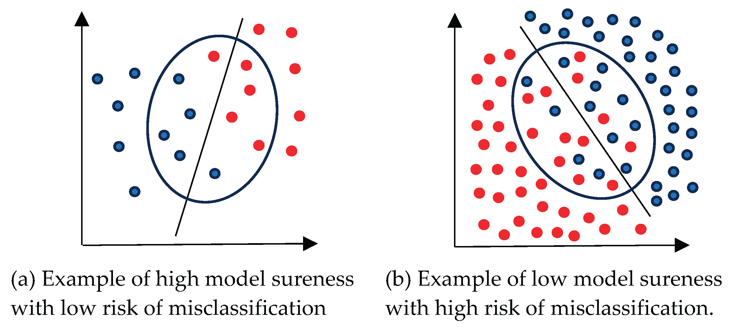
Figure 2.
Iris Versicolor (red) and Virginica (cyan) classes: illustration of pure and overlap areas visualized in heatmap (a) and Parallel Coordinates (b). In (b) in the last column cases are ordered by the values of a Linear Discriminant Analysis (LDA) classifier F(x) trained using all Versicolor and Virginica cases.
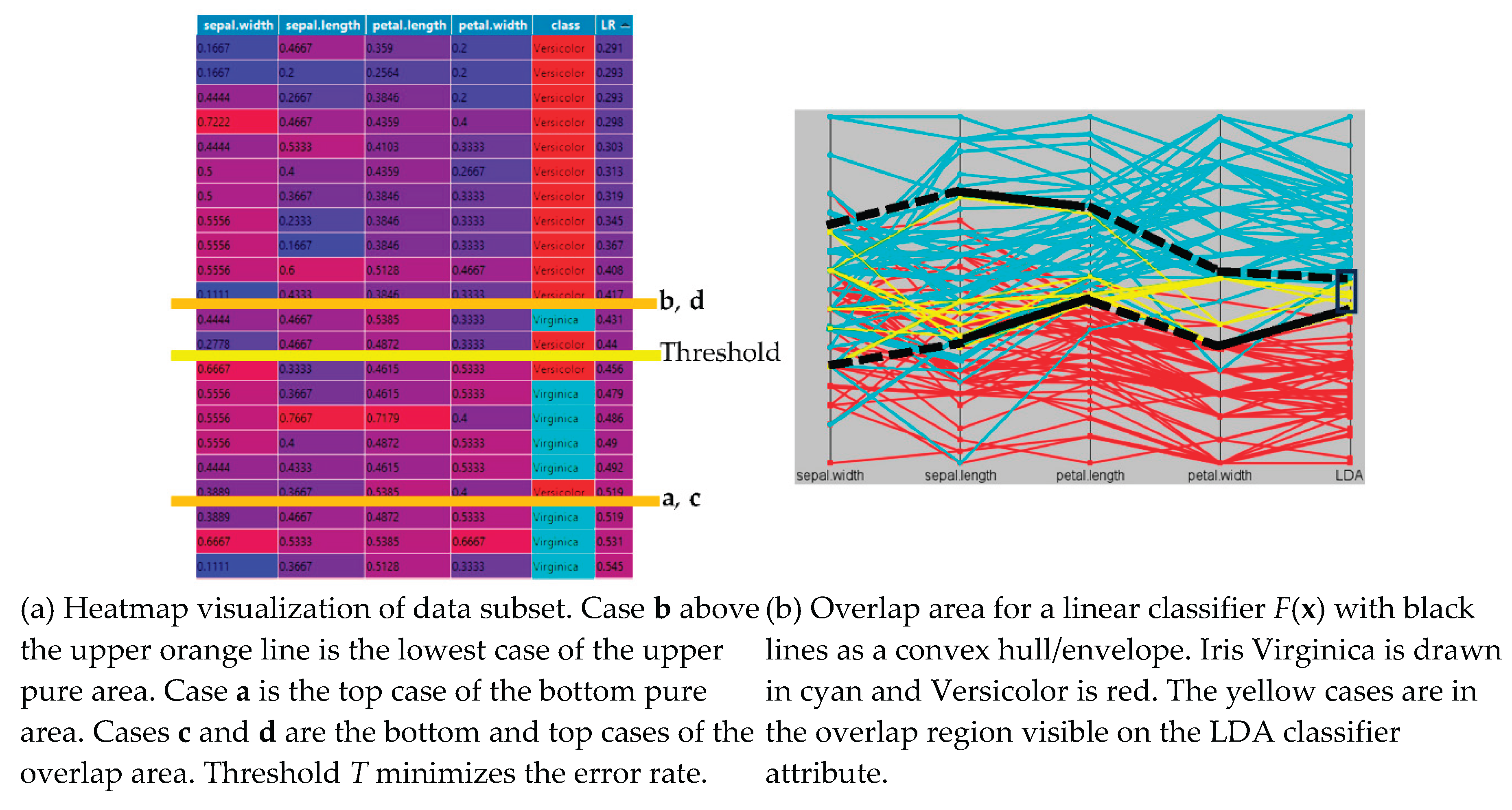
Figure 3.
Examples of different model sureness show how the addition of one case changes an easy classification scenario to a difficult one.
Figure 3.
Examples of different model sureness show how the addition of one case changes an easy classification scenario to a difficult one.
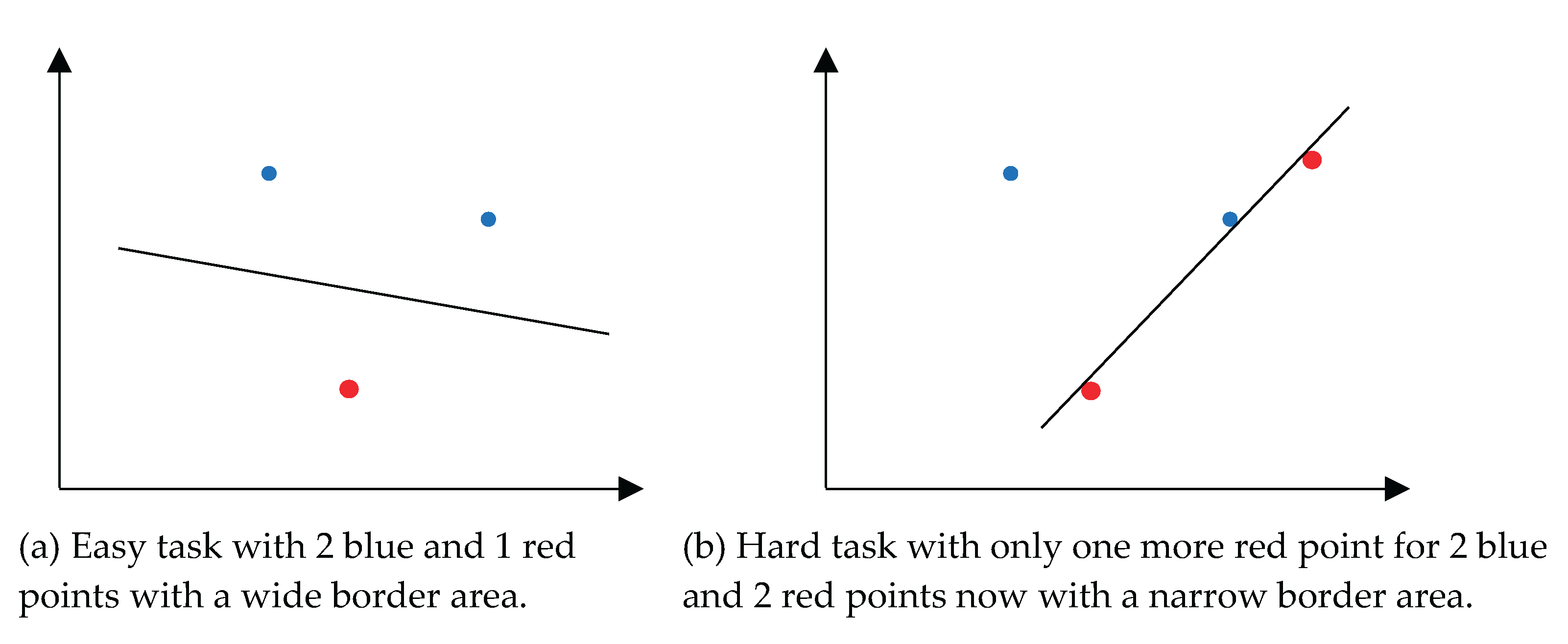
Figure 4.
Flowchart of the overall Model Sureness evaluation process. Iterates model training and evaluation under the threshold stopping criteria is reached by the trained model, such as 95% accuracy on the test data.
Figure 4.
Flowchart of the overall Model Sureness evaluation process. Iterates model training and evaluation under the threshold stopping criteria is reached by the trained model, such as 95% accuracy on the test data.
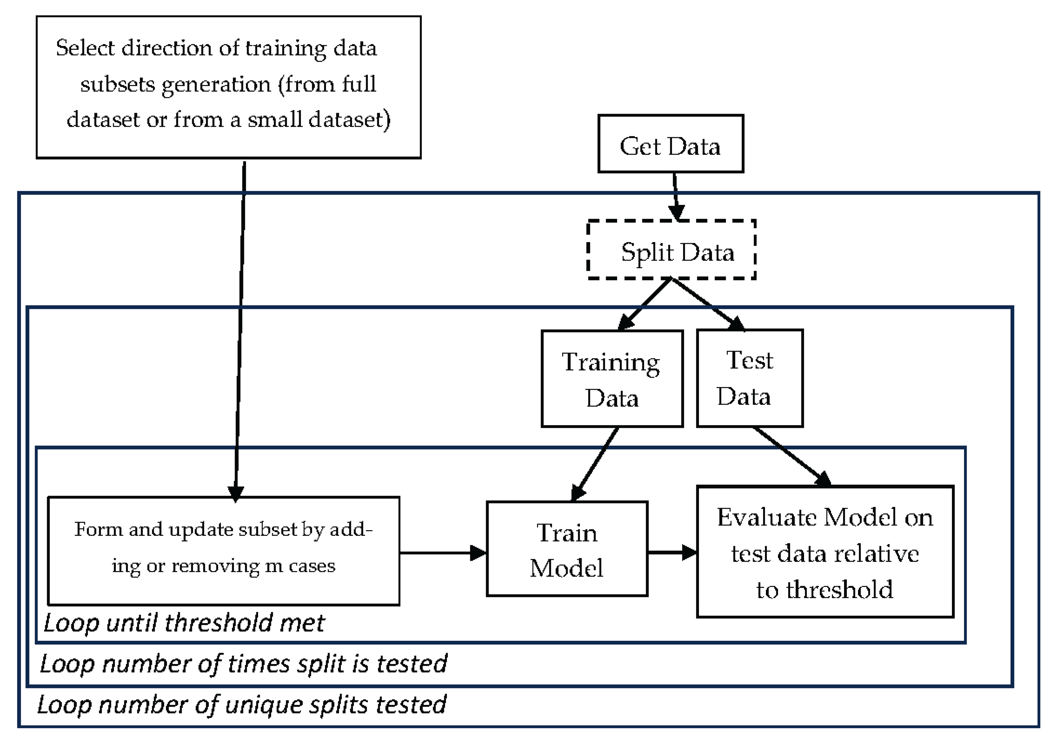
Figure 5.
MNIST actual computation time in minutes of 10 tests totaled for each m value using sureness testing with linear Support Vector Machine classifier and steps from 25 to 200 cases.
Figure 5.
MNIST actual computation time in minutes of 10 tests totaled for each m value using sureness testing with linear Support Vector Machine classifier and steps from 25 to 200 cases.
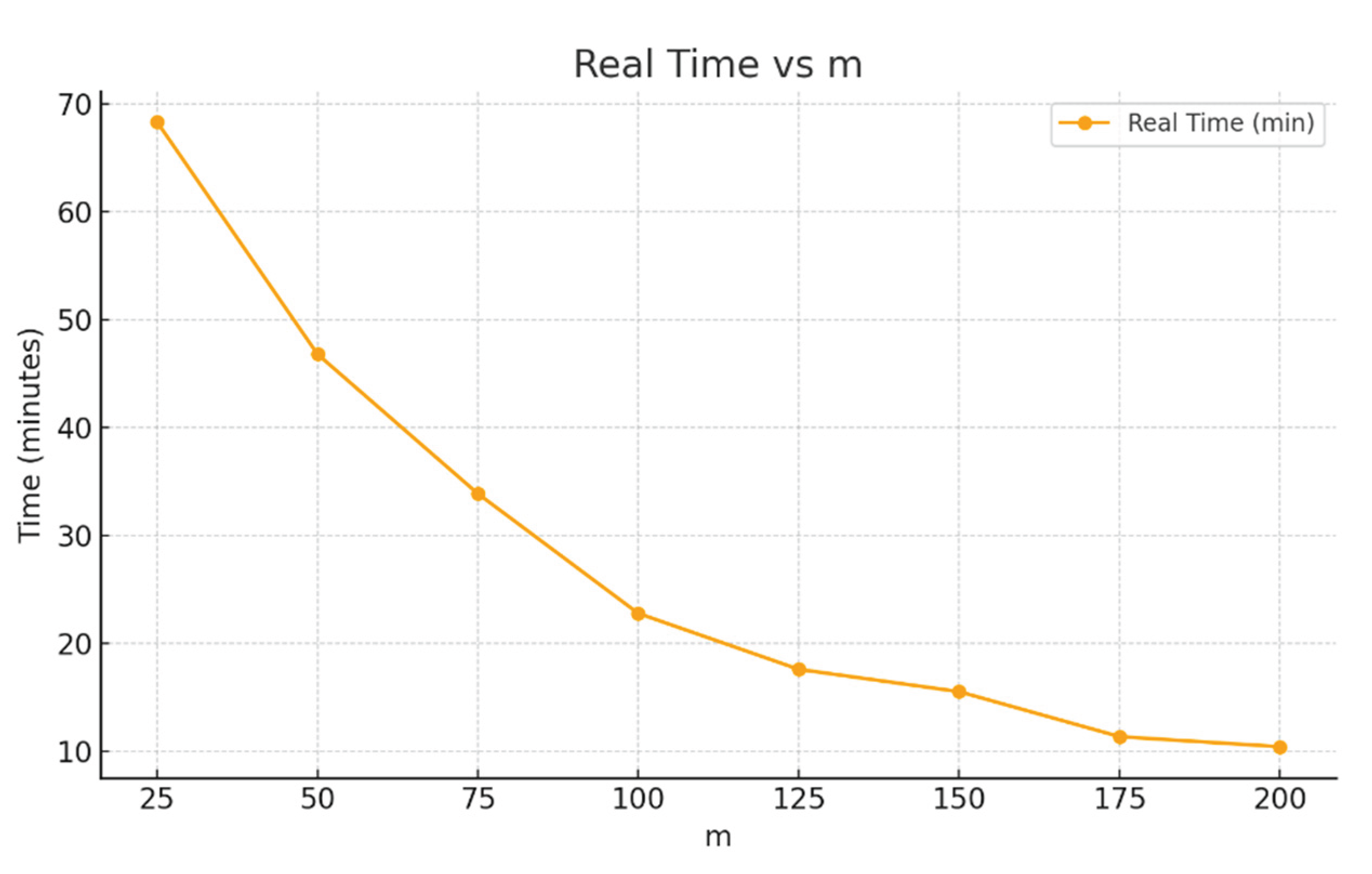
Figure 6.
Line graph showing the time to compute on the Fisher Iris data with 70% of 150 cases in training data. Using 100 splits for 100 iterations of model training each split.
Figure 6.
Line graph showing the time to compute on the Fisher Iris data with 70% of 150 cases in training data. Using 100 splits for 100 iterations of model training each split.
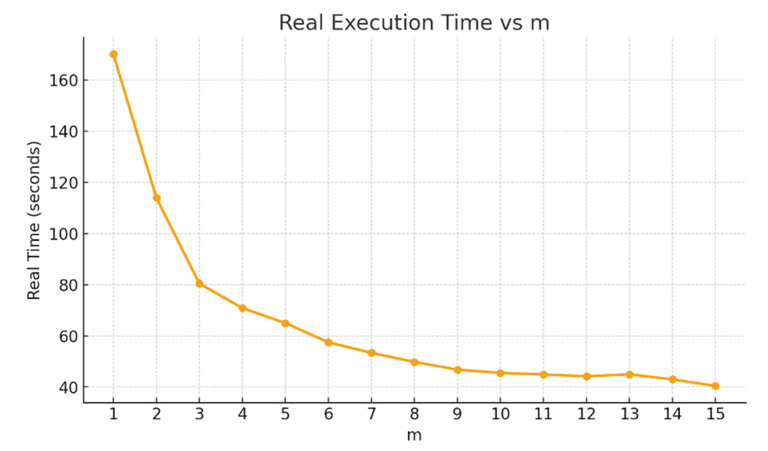
Figure 7.
Line graph showing the results for WBC9 data using 70% of 683 cases to train on 100 splits and 100 iterations of model training each split. The size of step m varied from 1 to 15 cases (0.15% and 2.2% of the dataset respectively).
Figure 7.
Line graph showing the results for WBC9 data using 70% of 683 cases to train on 100 splits and 100 iterations of model training each split. The size of step m varied from 1 to 15 cases (0.15% and 2.2% of the dataset respectively).
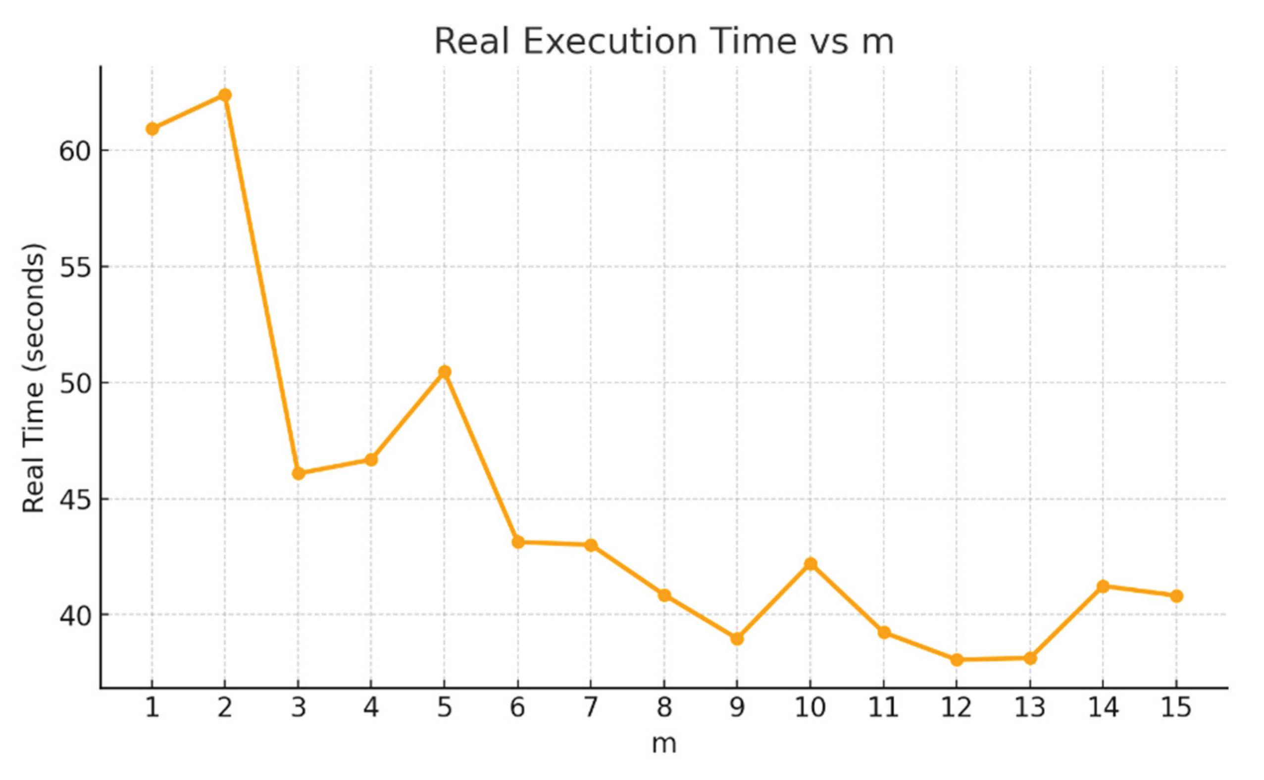
Figure 8.
Line graphs of the min, average and max cases needed for 10 tests on MNIST data from Figure 5.
Figure 8.
Line graphs of the min, average and max cases needed for 10 tests on MNIST data from Figure 5.
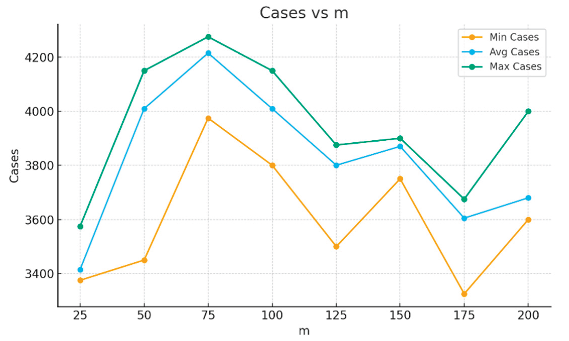
Figure 4.
Examples of best and worst subsets of training Iris data visualized in Parallel Coordinates.
Figure 4.
Examples of best and worst subsets of training Iris data visualized in Parallel Coordinates.
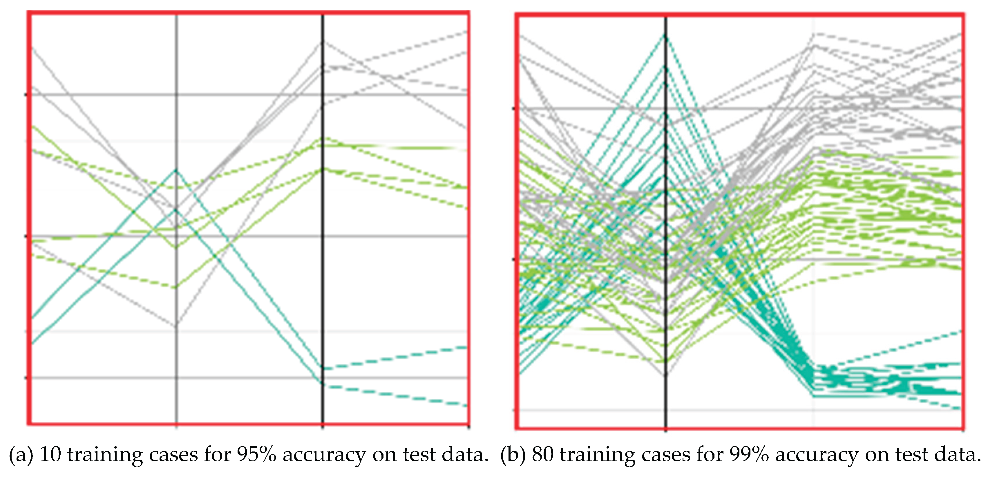
Figure 5.
Parallel Coordinates plot sequence that shows the growing training data set by 5 cases each time. The last subplots are the test data from experiment in Table 1. The red rectangles show the cases needed to get the required accuracy threshold of 95%.
Figure 5.
Parallel Coordinates plot sequence that shows the growing training data set by 5 cases each time. The last subplots are the test data from experiment in Table 1. The red rectangles show the cases needed to get the required accuracy threshold of 95%.
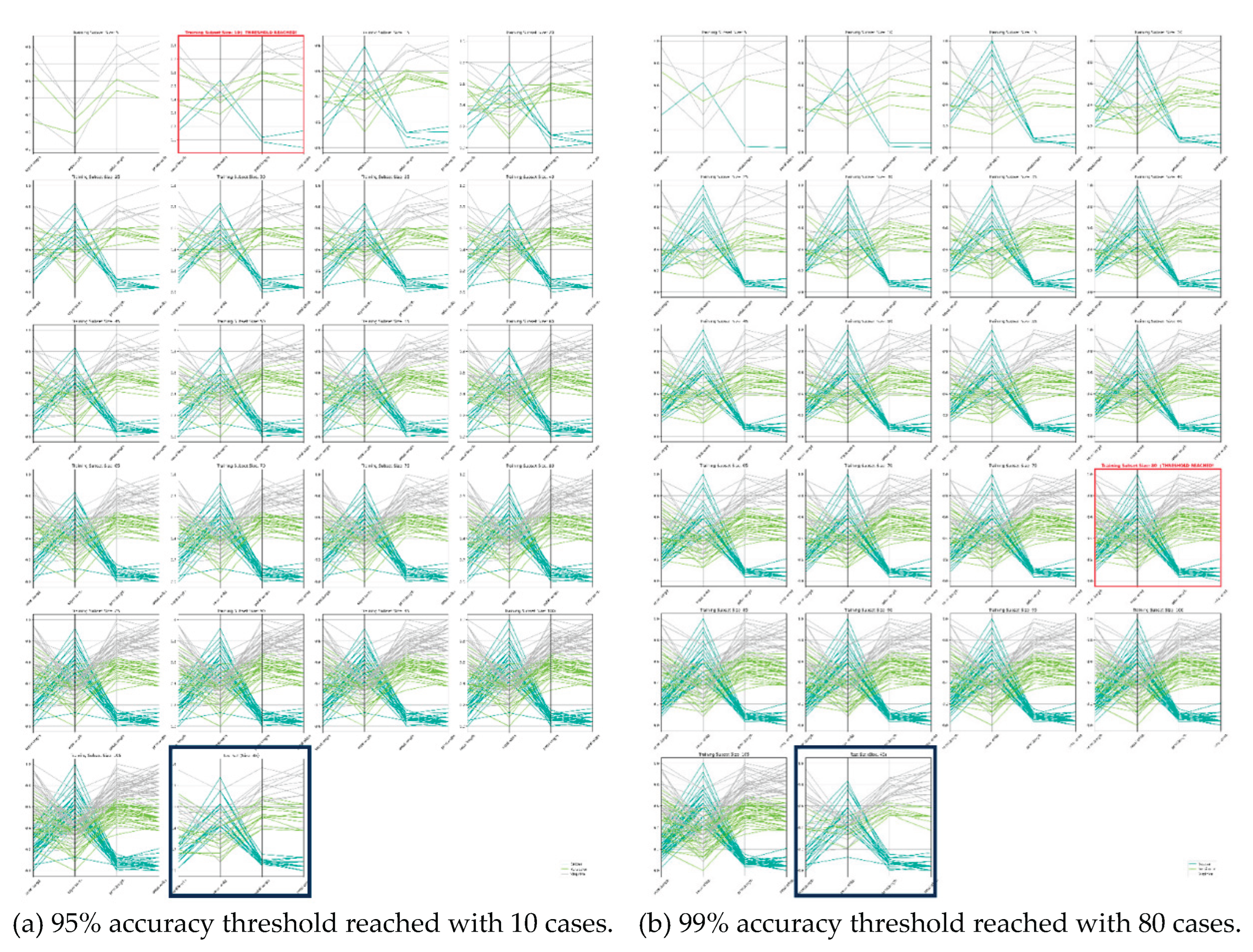
Figure 6.
Visualization in Parallel Coordinates of the 9,600-case subset. Each digit/class is in a subplot; the last subplot shows all digits together.
Figure 6.
Visualization in Parallel Coordinates of the 9,600-case subset. Each digit/class is in a subplot; the last subplot shows all digits together.
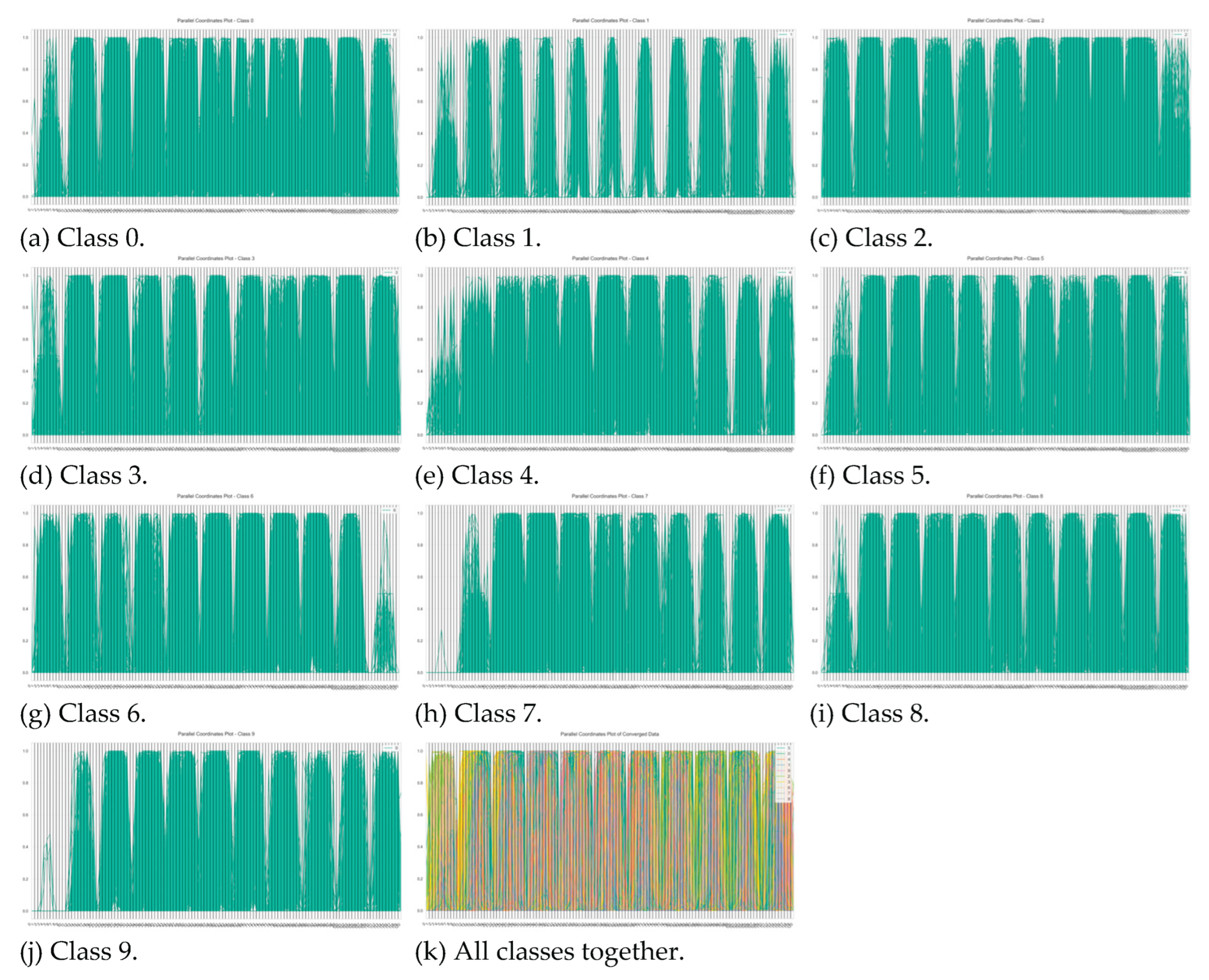
Figure 7.
Just the class 2 and 7 plots for a binary classification visual comparison.
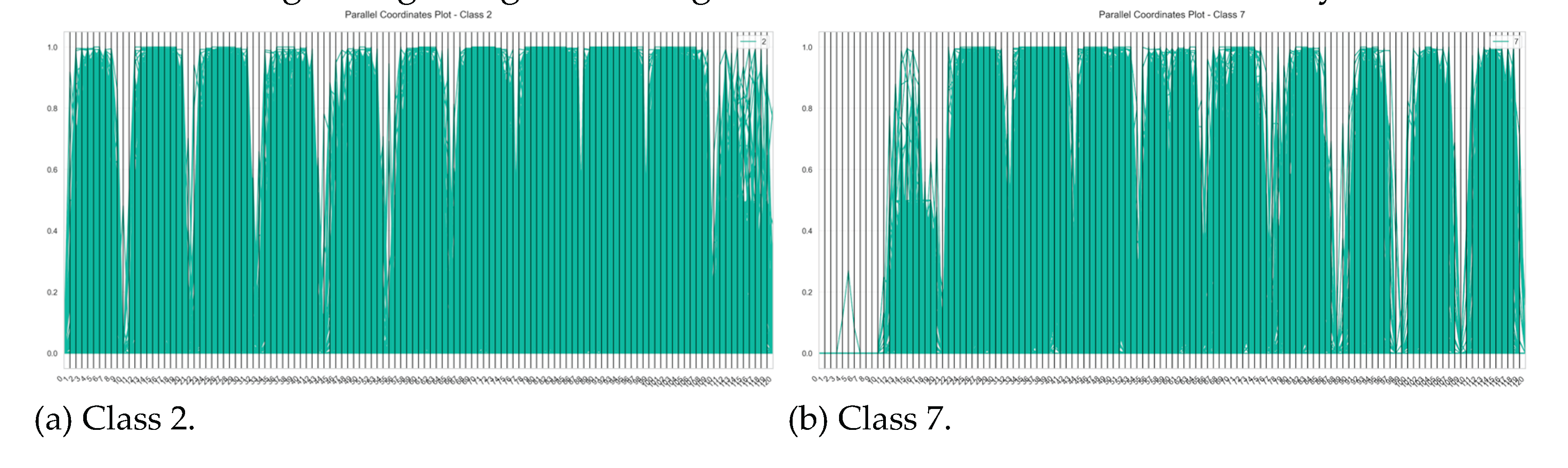
Figure 8.
2-D scatterplot visualizations of all 60,000 training data cases in top two plots, and the 9,600 case reduced training data set in the bottom two.
Figure 8.
2-D scatterplot visualizations of all 60,000 training data cases in top two plots, and the 9,600 case reduced training data set in the bottom two.
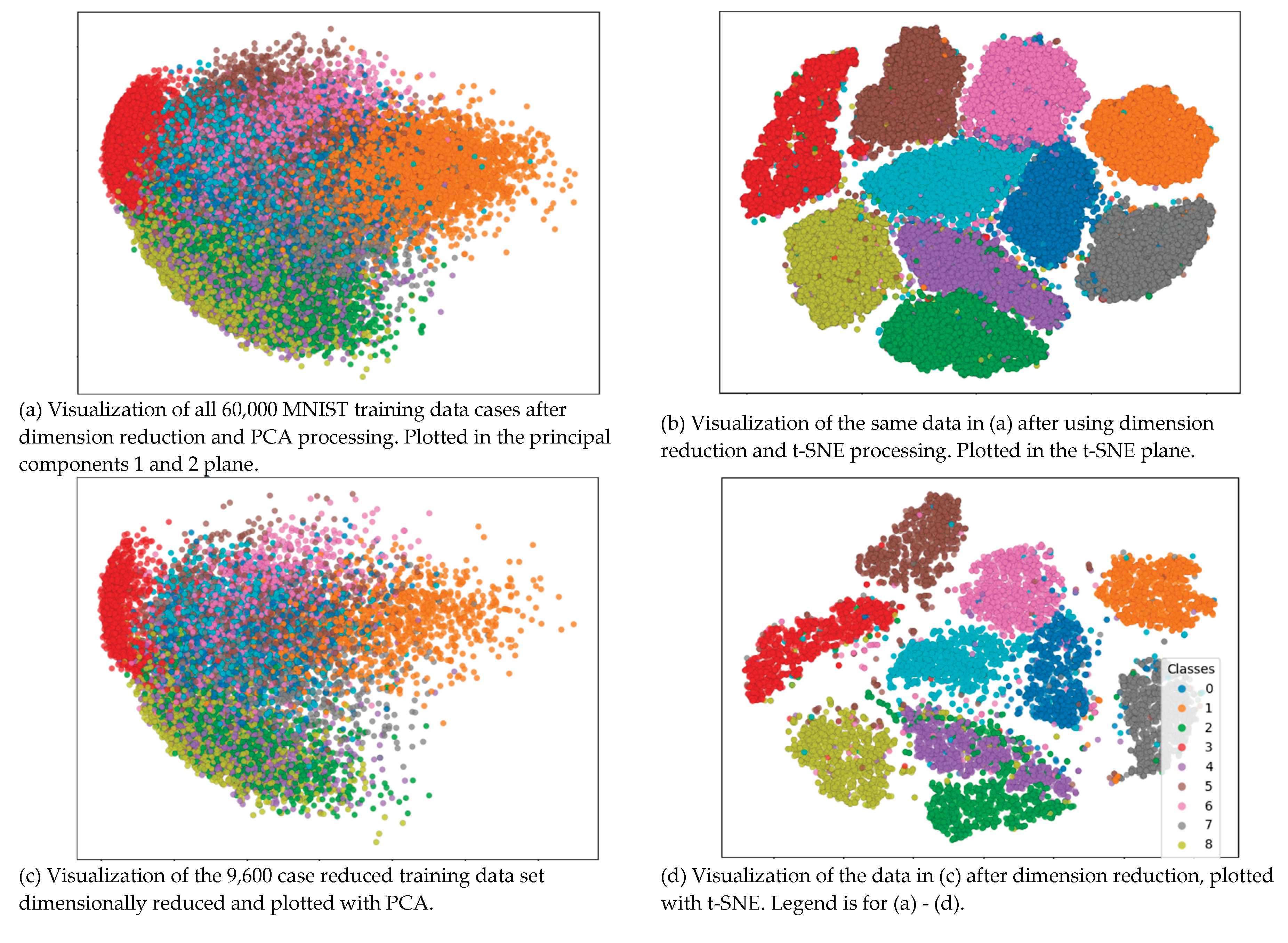
Figure 9.
Visualization of the centroids from the full data on top two plots, and the reduced data in bottom two.
Figure 9.
Visualization of the centroids from the full data on top two plots, and the reduced data in bottom two.
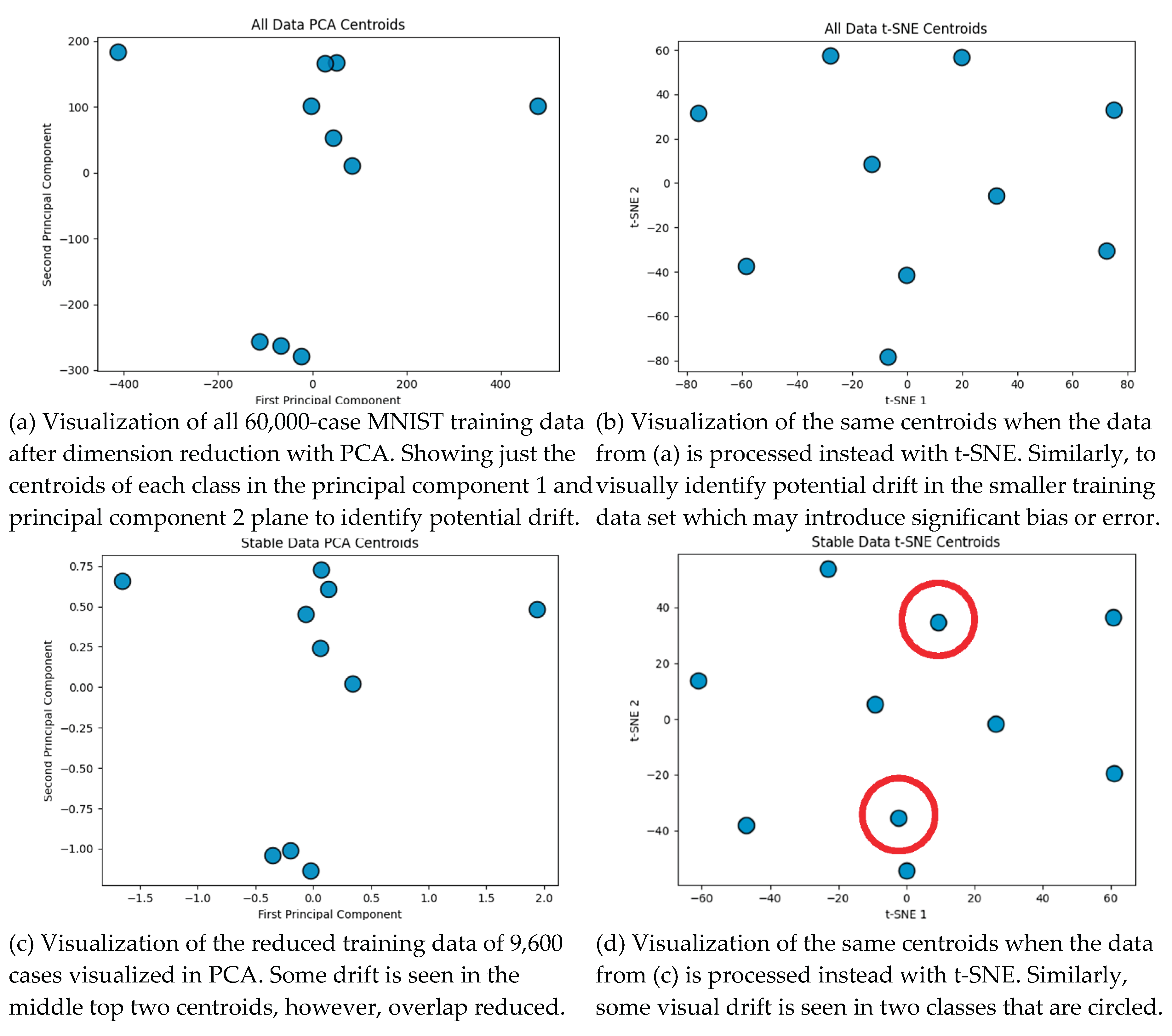
Figure 8.
Visualizations in Parallel Coordinates of the 2,800 cases that were used to train the model that had the top accuracy. Each subplot shows the class individually, the last subplot shows all classes overlaid. This shows a 2,800-case subset of the 60,000 original sufficient for training a 95.36% accurate single CNN classifier.
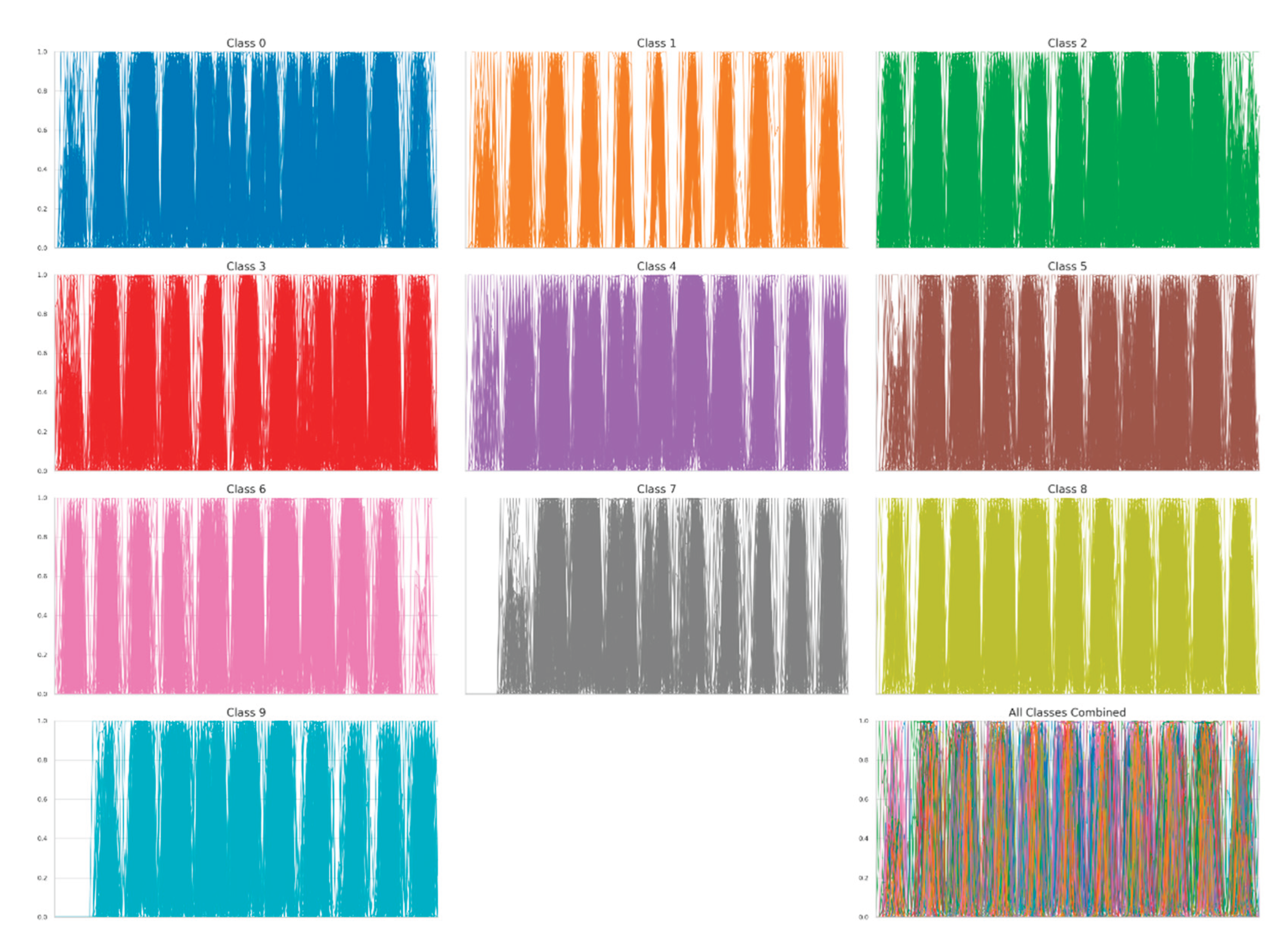
Table 1.
SVM Linear classifier and MSMDS algorithm on the Fisher Iris data with all three classes of 150 total cases, using a ten-case step, 70:30 split (105 training cases:45 test cases), and an accuracy threshold of 95%.
Table 1.
SVM Linear classifier and MSMDS algorithm on the Fisher Iris data with all three classes of 150 total cases, using a ten-case step, 70:30 split (105 training cases:45 test cases), and an accuracy threshold of 95%.
| Characteristics | Number of SVM Linear Iterations | ||
|---|---|---|---|
| 10 | 100 | 1,000 | |
| Mean Cases Needed | 37.8 ± 22 [15.8, 59.8] |
31.6 ± 16.5 [15.1, 48.1] |
31.8 ± 18.5 [13.3, 50.3] |
| Mean Cases Needed % | 36% ± 21% [15%, 59%] |
30.1% ± 15.7% [14.4, 45.8] |
30.3% ± 17.6% [12.7, 47.9] |
| Min Cases Needed | 10 | 10 | 10 |
| Min Cases Needed % | 9.5% | 9.5% | 9.5% |
| Max Cases Needed | 90 | 90 | 100 |
| Max Cases Needed % | 85.7% | 85.7% | 95.2% |
| Mean Model Accuracy | 0.953 ± 0.035 | 0.959 ± 0.026 | 0.961 ± 0.026 |
| Convergence Rate | 9 / 10 = 90% | 93 / 100 = 93% | 919 / 1000 = 91.9% |
|
Mean Model Sureness measure ratio |
1 - 0.36 = 0.64 | 1 - 0.301 = 0.699 | 1 - 0.303 = 0.697 |
* The Convergence Rate is measured by the ratio of the number of times the model was considered as “sure” (under given accuracy threshold) relative to the total number of iterations ran.
Table 2.
Results of measuring Model Sureness on Fisher Iris data with all three classes for 150 total cases, using LDA algorithm, and 70:30 split. with the MSMDS algorithm adding 10 cases from 70:30 split to threshold of 95%.
Table 2.
Results of measuring Model Sureness on Fisher Iris data with all three classes for 150 total cases, using LDA algorithm, and 70:30 split. with the MSMDS algorithm adding 10 cases from 70:30 split to threshold of 95%.
| Characteristics | Number of LDA Iterations | ||
|---|---|---|---|
| 10 | 100 | 1,000 | |
| Mean Cases Needed | 19 ± 5.4 [13.6, 24.4] |
21.3 ± 14.3 [7, 35.6] |
21.1 ± 14.5 [6.6, 35.6] |
| Mean Cases Needed % | 18.1% ± 5.1% [13%, 23.2%] |
20.3% ± 13.6% [6.7%, 33.9%] |
20.1% ± 13.8% [6.3%, 33.9%] |
| Min Cases Needed | 10 | 10 | 10 |
| Min Cases Needed % | 9.5% | 9.5% | 9.5% |
| Max Cases Needed | 30 | 100 | 100 |
| Max Cases Needed % | 28.6% | 95.2% | 95.2% |
| Mean Model Accuracy | 0.980 ± 0.018 | 0.977 ± 0.021 | 0.977 ± 0.02 |
| Convergence Rate | 10 / 10 = 100% | 99 / 100 = 99% | 981 / 1000 = 98.1% |
|
Mean Model Sureness measure ratio |
1 – 0.181 = 0.819 | 1 – 0.203 = 0.797 | 1 – 0.201 = 0.799 |
Table 3.
Results of evaluating the Fisher Iris with Versicolor and Virginica classes by the Additive Hyperblock Grower (AHG) algorithm, the HBs have been grown with IMHyper algorithm [92].
Table 3.
Results of evaluating the Fisher Iris with Versicolor and Virginica classes by the Additive Hyperblock Grower (AHG) algorithm, the HBs have been grown with IMHyper algorithm [92].
| Iteration | Cases in Training data | Hyperblock Count | Average Hyperblock Size |
Next Misclassified |
|---|---|---|---|---|
| 1 | 5 | 2 | 2.5 | N/A |
| 2 | 5 | 2 | 2.5 | 0/5 |
| 3 | 10 | 2 | 5 | 0/5 |
| 4 | 15 | 2 | 7.5 | 0/5 |
| 5 | 20 | 2 | 10 | 0/5 |
| 6 | 25 | 2 | 12.5 | 0/5 |
| 7 | 30 | 2 | 15 | 0/5 |
| 8 | 35 | 2 | 17.5 | 0/5 |
| 9 | 40 | 2 | 20 | 0/5 |
| 10 | 45 | 2 | 22.5 | 0/5 |
| 11 | 50 | 2 | 25 | 0/5 |
| 12 | 55 | 2 | 27.5 | 0/5 |
| 13 | 60 | 2 | 30 | 0/5 |
| 14 | 65 | 2 | 32.5 | 0/5 |
| 15 | 70 | 2 | 35 | 0/5 |
| 16 | 75 | 2 | 37.5 | 0/5 |
| 17 | 80 | 2 | 40 | 0/5 |
| 18 | 85 | 2 | 42.5 | 0/5 |
| 19 | 90 | 2 | 45 | 0/5 |
| 20 | 95 | 2 | 47.5 | 0/5 |
| 21 | 100 | 2 | 50 | 0/5 |
Table 5.
Results from the MNIST data with k-NN classifier, adding 100 cases each iteration, until 95% accuracy.
Table 5.
Results from the MNIST data with k-NN classifier, adding 100 cases each iteration, until 95% accuracy.
| Number of k-NN Iterations | ||
|---|---|---|
| Characteristics | 10 | 100 |
| Mean Cases Needed | 9,600 | 9,600 |
| Mean Cases Needed % | 16% | 16% |
| Min Cases Needed | 9,600 | 9,600 |
| Min Cases Needed % | 16% | 16% |
| Max Cases Needed | 9,600 | 9,600 |
| Max Cases Needed % | 16% | 16% |
| Mean Model Accuracy | 0.972 | 0.972 |
| Convergence Rate | 10/10 = 10% | 100/100 = 100% |
|
Mean Model Sureness measure ratio |
1 – 0.16 = 0.84 | 1 – 0.16 = 0.84 |
Table 6.
Listing of the case per class distribution of the smaller MNIST training datasets for k-NN with k = 3 to yield a 97.2% accurate model.
Table 6.
Listing of the case per class distribution of the smaller MNIST training datasets for k-NN with k = 3 to yield a 97.2% accurate model.
| Cases Per Class Label | Case Count | Percentage |
|---|---|---|
| 0 | 954 | 9.94% |
| 1 | 1,088 | 11.33% |
| 2 | 946 | 9.85% |
| 3 | 985 | 10.26% |
| 4 | 953 | 9.93% |
| 5 | 834 | 8.69% |
| 6 | 976 | 10.17% |
| 7 | 1,029 | 10.72% |
| 8 | 899 | 9.36% |
| 9 | 936 | 9.75% |
Table 7.
CNN accuracy on all MNIST data. .
| Training Data (all 60,000 training MNIST cases) | Accuracy on all Test Data (10,000 cases) |
|---|---|
| Data 28x28 (784-D data) | 99.57% |
| Data 11x11 (121-D data by 3 pixels crop edges and average pooling of 2x2 kernel, 2 stride) | 99.34% |
Table 8.
Results of model accuracy given various reduced training data subsets.
| Accuracy on all test data | Sample Count |
|---|---|
| 95.36% | 2,800 |
| 96.25% | 3,200 |
| 95.20% | 2,500 |
| 95.93% | 2,700 |
| 96.79% | 2,800 |
Disclaimer/Publisher’s Note: The statements, opinions and data contained in all publications are solely those of the individual author(s) and contributor(s) and not of MDPI and/or the editor(s). MDPI and/or the editor(s) disclaim responsibility for any injury to people or property resulting from any ideas, methods, instructions or products referred to in the content. |
© 2025 by the authors. Licensee MDPI, Basel, Switzerland. This article is an open access article distributed under the terms and conditions of the Creative Commons Attribution (CC BY) license (http://creativecommons.org/licenses/by/4.0/).
Copyright: This open access article is published under a Creative Commons CC BY 4.0 license, which permit the free download, distribution, and reuse, provided that the author and preprint are cited in any reuse.


