
Submitted:
05 July 2025
Posted:
07 July 2025
You are already at the latest version
Abstract
Crack growth is, in theory, very well known, and crack initiation is also quite well described and proven by different physical explanations and mathematical models in the literature. However, crack incubation is not a well-investigated phenomenon, especially if this phenomenon relates to the question of why.
So, teachers and students for understanding need logical explanations. This paper aims to focus on this area, the crack incubation and initiation field, and explain it with an appropriate model, included in the context of the already developed AI expert system (ES). The application of this advanced ES developed for education will be shown in the design example and the dimensioning and optimizing gears and gearing. The individual teachers, using this ES can successfully plan and execute optimal lessons for various subjects using. The presented mathematical model will enable the teachers to have a complex approach to teaching, but it will also be helpful for the self-learning and self-training of the students.
Keywords:
principle of universality
; fracture mechanics
; mathematical models
; crack incubation
; expert system
; gear assemblies
; computer aided design
1. Introduction
Structural design begins with identifying a need and concludes, through a repeated cycle of preliminary design, analysis, and detailed design, by meeting that need. Recently, many efforts have been made to create integrated structural analysis and design systems. In the 1960s, Feigenbaum and colleagues proposed that the effectiveness of artificial intelligence (AI) techniques could be improved by incorporating domain knowledge. This led to the development of presented expert systems (ES) [1,2]. This paper only focuses on a segment of this system for training in designing gear assemblies, specifically the heuristic component of the mathematical model, connected mainly with context (according to Figure 1).
To deal with materials in the macro world, we have a series of known and reliable mathematical models shown in the second part of the paper. The problem that we are trying to solve in this paper deals with a complex and poorly processed area where we have to deal with the material at the nano and micro levels [2]. Modeling the quantum mechanical interactions of thousands and thousands of molecules has been a long-held ambition for computational material scientists, yet this remains unfeasible. At this time, the limitations necessitate a trade-off: compromise on system size, as with the Density Functional Theory (DFT) methods that are limited to around 100 atoms, or sacrifice accuracy and the modelled chemistry level, as is the case with empirical potentials [3]. Our paper, which could also be titled “From nano to macro: Introduction to atomistic modelling techniques”, provides an introduction to a new generation of reactive force fields, centering on the reactive force fields (ReaxFF) theory [4]. Reactive force fields mark a major advancement in bridging the divide between QM (DFT) and empirical nonreactive potentials. They achieve this by enabling the modelling of complex chemical reactions, while remaining computationally manageable and applicable for systems exceeding 1E4 atoms. This paper reviews the core concepts of ReaxFF and compares the underlying theories and approaches to classical, nonreactive formulations. Our findings demonstrate that the incorporation of concepts like charge flow, continuous energy during reactions, changing bond orders, and shielded nonbonding van der Waals and ionic interactions allows us to describe, with quantum mechanical accuracy, the properties of complex, hierarchical materials [1,4].
At its core, crack growth is an atomic-scale phenomenon, characterized by the severing of atomic bonds to create new surface area [1,3]. Nevertheless, the breaking of bonds at the crack’s tip (or even at the non-existent tip) accounts only for a small fraction of the energy dissipation during crack growth in a typical structural metal because most of the energy dissipation is associated with continuum plasticity. Despite that, the breaking of bonds at the tip is often the dominant factor in the fracture process. Take, for instance, the boundary condition where surface energy effectively goes to zero. Under such conditions, a crack will grow with even an infinitesimally small load.
Information regarding the material, geometry, necessary surface machining, and tolerances is automatically transferred from the CAD process. For gears, this includes the characteristics relevant for their subsequent manufacturing and heat treatment. An independent, interactive post-processor generator is also a part of this system. Moreover, the system includes experimental design, statistical evaluation of measurement data, finite element calculations for tool strength analysis, and final design optimization. The results obtained are then accumulated in a database, which is accessible to the user. The final result would consist of an optimal gear pair/gearing, along with the material selection instructions, mechanical manufacture, thermal treatment, lubrication method, manufacturing, etc. During the process, students must demonstrate knowledge and understanding by answering various questions [1,2].
2. Intelligence System in Schools
At the time of writing this article, education in modern society is undergoing a drastic transition. Various authorities believe this stems from the significant limitations of the traditional lecture approach, which still assigns a passive role to the student. However, recently and even more intensely after the pandemic period, a wave of innovation, stimulated by information technology (IT), promises to revolutionize and revitalize/transform our schools. Teaching methods based on outcomes, e-learning at a distance, home schooling, collaborative group work, Generative Artificial Intelligence (GenAI), and large language models (LLM) are becoming increasingly prevalent in today's educational milieu [5]. These changes are proving so effective that they signal the need for a major reconceptualization/transformation of the learning process. The objective of high school, university, and even some vocational programs must be cultivating the essential drive for curiosity, for learning to learn, and critical thinking/critical evaluating/critical decision making in students. To achieve this, students must be involved as active, self-directed learners. This necessitates the provision of robust new kinds of technology to establish an information-rich and intelligent learning environment, where students and teachers alike can navigate and explore different informational superhighways [5].
2.1. Knowledge-Based ES and Other Intelligent Systems
Knowledge-based expert systems (ES) are interactive computer programs that provide expertise and advice across various tasks [1,2]. They are typically comprised of the following three components:
- Of the behavior of the problem domain,
- Context, in all three areas in Linguistic context and natural language processing (NLP, in users’ context, which considers users’ data as past interest or behavior, allowing personalized experiences, and in situation context, which could be a personal assistant, etc. Context is crucial for the effectiveness of AI systems and their responses to complex inquiries.
- Inference Mechanism (heuristic), which monitors program execution by utilizing the knowledge-base to modify Context in all three areas, generating a workspace for the problem established by the Inference Mechanism using the user-provided information and the knowledge-base or from the ML algorithm.
Aside from the three main modules, the system should also implement a graceful:
- User Interface;
- Explanation Facility;
- Knowledge-Acquisition Module, as schematically shown in Figure 1.
For example, an ES could also be constructed for mechanical engineering to analyze data, and then simulate the design and optimization of gear transition, as in our case. An ES system could adapt its questions and tutoring to match the student's comprehension level.
3. Results
Standard calculations are limited to a single engaged gear pair, which means it is impossible to take into account the side effects like the service life of bearing, shafts, etc. Thus, we have, in our ES, included an AI-based optimizer and a genetics algorithm. Realizing an optimization algorithm for a generalized gear assembly model requires the use of procedures for separating independent and dependent variables, thus taking into account the given geometric constraints. The goal is to determine the shortest evaluation time for the evaluation of the dependent variables of individual gear assembly variants. All such “tools” must be used to develop students' logical minds and understanding [2,6].
The ES is connected to suitable knowledge bases or an ML algorithm that compiles extensive theoretical knowledge and experience of a specific domain. During the gearing design process, it is essential to ensure that it functions throughout its specified service life. Other factors are minimizing gearing size and its components to ensure minimum weight, smaller material use, and a lower price [1,5]. The overall synthesis process includes:
- differentiating between dependent and independent parameters,
- gearing model construction,
- an iterative process to determine the optimal design, with successive model analysis.
Several criteria may be used for optimization. The minimum total volume of the gears' pitch cylinders is often used [1]:
The optimization algorithm is aimed at finding a combination of parameters – module mn, number of teeth z, tooth width b, angle of helical tooth o, materials, and heat treatments – that results in the lowest possible chosen function value F. P denotes the function of all other influences. The genetic algorithm only requires information about the selected points' value, without any additional details regarding the selected function. The algorithm considers the total reproduction effect, crossbreeding, and mutation. When the three influencing variables are combined, the genetic algorithm’s basic theorem is obtained:
We can summarize the optimization process as follows:
- A small, random initial population is chosen.
- Using genetic operators and taking into account the selected local criteria, the convergence of the population is affected.
- The new population is determined by integrating the most successful members of the old population, while the remaining members are randomly selected.
- If the global convergence criterion is fulfilled, the process is terminated, or
- We go back to point 2.
3.1. Calculating Service Life
Let us now focus only on the model of determining the potential crack and its propagation at the atomic/nano level. We will divide this area into two parts: the crack incubation and the crack initiation part.
3.1.1. Crack Without a Crack – Crack Incubation
What about non-existent cracks? Why do they begin to form? We will attempt to address this question by using the theory of universality. The mystery of universality can be found in the everyday stuff of our natural world, from gases, liquids, solids, and even in complex systems like ecosystems or the economy. Universality offers a fresh understanding of how ostensibly very distinct things can behave in the same way. What’s beautiful is that these things do not necessarily have to exist in the physical sense. This includes mathematical entities. Thus, when modelling a crack incubation (close to the critical point), one does not have to ensure accuracy in representing the interaction between every neighbouring atom or every neighbouring grain in solids. A technically complex system’s behaviour emerges from the interactions of individual elements that constitute it. Following universality, the exact nature of the constituting elements and how they interact are often not important. »Universality gives us confidence, that we really can model and understand complex system«. To start using this theory, we only have to meet one condition: the system must be in a critical state. Mathematically speaking, this critical state is what physicists refer to as a power law [1,2,7].
Picture one hundred grains, modelled as matchsticks and positioned alongside a single line. The length of each measured matchstick indicates grain fitness and is represented by a random number between 0 and 1, generated using the Monte Carlo method. The model progresses step by step. First, the lowest fitness grain breaks, i.e., we discard the shortest matchstick and replace it with a new one, the length of which is, again, chosen at random, between 0 and 1. Additionally, the two closest neighbouring matches to this grain also break and are replaced in the same way. This roughly simulates how elements in the real world interact: one extinction can trigger others [1].
To simulate how a fracture propagates, one just has to repeat these steps again and again. Yet, despite its simplicity, the model displays remarkably complex behaviour. After numerous iterations, the technical system reaches a critical state, where the fitness pattern becomes self-similar. At least three elements are replaced after every step. However, after a series of cycles, the interplay of elements allows the crack to traverse the entire system in a chain reaction, which is known as crack propagation. If this is simulated by a computer, the models show crack propagation sorted by size, represented as the number of grains in the chain reaction, in a manner similar to how cracks are initiated and propagated in the real world. Once cracks begin to propagate, we are able to utilize various well-known short and long crack propagation models, as detailed in Chapter 4. In what follows, a potential universal mechanism that facilitates crack formation/nucleation will be introduced [3,4].
3.1.2 Potential Crack Nucleation Sites
A possible mechanism for “crack” nucleation sites in any structure, achieved through a symmetry-breaking phase transition, is presented below. Such cases are ubiquitous in nature in condensed matter systems. In addition, such configurations are very susceptible to various perturbations. Note that the current structure of the universe has been formed via a symmetry-breaking phase transition [8]. Therefore, the described phenomenon is broadly universal [9,10].
In any condensed matter system in general, the presence of impurities cannot be avoided. They often give rise to random-field (RF) type disorder, the impact of which has been intensively studied in magnetic systems [11,12] and recently also in various liquid crystal (LC) phases [13]. The latter can occur due to continuous symmetry breaking and a rich variety of phases and structures exhibiting practically all possible topological defect structures encountered in nature (e.g., even analogues of magnetic monopoles and cosmic strings) [14]. In case of translational order, ubiquitous topological defects are edge dislocations and screw dislocations. For example, several studies have recently been carried in twist grain boundary smectic phases [15] that are dominated by lattices of screw dislocations. Corresponding structures in magnetic systems are superconducting Abrikosov phases [16]. In the following section, we use the simplest possible minimal mesoscopic model to demonstrate the impact of RF type disorder on orientationally ordered crystalline phase structures. For this purpose, we consider only the orientational degree of freedom perturbed by impurities imposing RF-type perturbations.
Nematic ordering at the mesoscopic level using the uniaxial tensor order parameter can be described as [10,17]
Here stands for nematic director field, where s represents the uniaxial nematic order parameter, ⊗ is the tensor product, while is the unit tensor. The local average orientation of a rod-like molecule is represented by a unit vector , where both directions are equivalent. On the other hand, s determines the degree of orientational ordering. In case of rigid alignment of molecules along it holds that s=1. Absence of orientational ordering corresponds to s=0. We assume that impurities are uniformly distributed within the volume sample V and that their volume concentration is given by
Here, vim stipulates the volume of an impurity, while Nim counts their number within V. The relevant free energy terms read as [10,17]
The first volume integral is applied across the crystal body, while the 2nd surface integral applies to the impurity-crystal interfaces. The elastic term ensures spatially uniform ordering, and can be approximated by [10]
where L represents the temperature-independent elastic constant. The interfacial term is modelled by [A10]
The quantity W stands for positive anchoring strength constant, and presents locally preferred orientation, . This ansatz locally enforces to align along . In modelling, we assume that impurities are uniformly distributed with a concentration p, and that their orientational probability distribution is spatially isotropic. According to the Imry-Ma theorem [11], which is one of the foundations in statistical mechanics of disorder, we assume that the disorder could break the system into a domain-type pattern, characterized by the average domain size ξ. In the following, we estimate the value of ξ in the orientationally ordered phase where s>0.
For this purpose, we express the average domain free energy value ∆F within domain volume :
Here, and aim describe the number of impurities within the average domain and an impurity surface area, respectively. We assumed that . Such behaviour is universally expected for gauge-type continuum fields. In our case, the role of the gauge field is played by . The quantity
determines an average value of the 2nd Legendre polynomial and marks the spatial averaging over the domain volume. Note that, within each domain, the nematic director is roughly aligned alongside a similar symmetry-breaking direction, and that the orientational distribution of orientations within it is isotropic. Consequently, within an infinitely large domain, one would expect . Yet, in a finite domain and according to the central limit theorem of statistics, it holds that
The number Nr counts the frequency of random reorientations of with respect to average orientation within a domain. It holds
Where
stands for an average separation between neighbouring impurities, and d is the dimensionality of space. We obtain an expression for ξ by balancing elastic and interface energetic contributions in ΔF. This yields an Imry-Ma [11] type expression for the characteristic domain size
where D is the effective disorder strength. This expression was originally derived in magnetism and constitutes a basic ingredient of the Imry-Ma theorem. The theorem claims that for d<4, even infinitesimal RF-type effective disorder strength D breaks long-range ordering anticipated in the pure system and replaces it with a short-range domain-type pattern. In d=3, our modelling yields
From this derivation, one sees that these impurities within a system, in general, break the system into a domain-type pattern, where energy penalties are non-homogeneously distributed and localized at domain walls. Consequently, intermolecular interactions at domain walls are weakened and, at these sites, “cracks” are expected to nucleate or propagate if one imposes a large enough external strain on the system.
3.2. Model of Crack Initiation
When we know phenomena of intermolecular interactions at domain walls and we are able to calculate a “non existing” crack, i.e., cracks expected to nucleate, to determine the characteristics of these nucleation cracks, it is crucial for analytical models that the S-N curves to account for the dominant characteristics of the crack tip fields and the crack growth rate, which starts high but then diminishes [1,3]. This is possible by considering the separate regimes in the modified Kitagawa-Takahashi diagram, which significantly advances the understanding of short crack behaviour. This diagram shows the effect of defect size on the fatigue limit stress; see, e.g., Figure 3. When dealing with large defects, the stress allowed for infinite life has to be low, within the linear elastic fracture mechanics regime. Thus, the limiting condition is represented by a straight line with a slope of minus one-half of the threshold stress intensity factor ΔKth, so that
where Y(a/S) represents the shape factor [3], stands for the stress ratio, and ath stands for the threshold crack length. At the opposite extreme, i.e., for extremely small defects, the permissible stress level must correlate to the fatigue limit of an uncracked specimen. The Kitagawa-Takahashi diagram illustrates the behaviour observed between these two extremes. We know that a larger dataset leads to more accurate results. Using a random number generator, the number of input data can be numerically expanded, and, based on the expanded dataset, we can calculate the new mean value that does not deviate from the original value by more than the prespecified standard deviation.
For crack initiation areas, we utilized the theory of continuously distributed dislocations in combination with crystal limits for analysing crystallographic slip deformations before the tip of a short fatigue crack, and we developed an appropriate model based on it [1,18]. Stress due to dislocations can lead to either the slip of an inclusion or the generation of a vacancy. Dislocations can converge on any obstacle to the slip, resulting in their spatial concentration. This leads to the formation of microcracks or crack growth through the convergence of the remaining dislocations. Our model for microcrack initiation and propagation utilizes the abovementioned assumptions.
The edge dislocation is the boundary between the region where the slip occurred and the region where the slip did not occur, as illustrated in Figure 4. If edge dislocation occurs, the free energy of a crystal increases. To perform this calculation, consider a cylindrical crystal of length l that has a spiral dislocation with its Burgers vector positioned alongside its axis. The Burgers vector b represents the shift size and corresponds to the total distance between atoms within a crystal lattice. For this cylindrical crystal with radius r and thickness dr, the energy for unit volume is
where γro corresponds to the elastic stress in the thin coil. We can determine the deformation energy by integrating equation (14):
According to equation (15), the energy is proportional to the dislocation length. The deformed dislocation produces linear stress T, which is a vector that can be determined as:
This allows us to calculate the relevant shear stress:
and the integral equation is derived for equilibrium [4]:
where corresponds to an edge dislocation, to spiral dislocation, and G to the shear modules.
Muskhelishvili previously demonstrated the solution to this integral equation in 1946 [1]. So, we can present the general notation of this distribution function in a more simplified and compact form as:
where is the dimensionless co-ordinate of the crack tip.
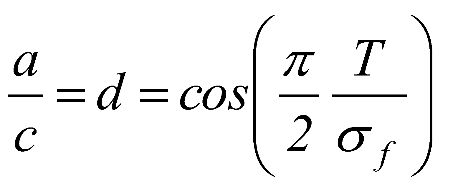
When calculating crack propagation, the most important parameter is the stress concentration before the crack, or more accurately, just before the crack expands to include the plastic zone. So, the additional stress for the point is:
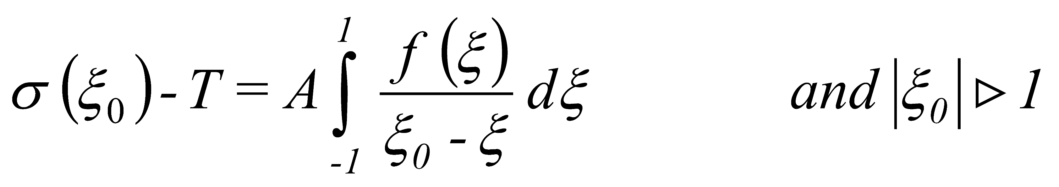 (20)
(20)Solving the integral equation (20) using the distribution function (19) and considering that value d (location of the initial crack tip) ranges from 0 to 1 gives us:
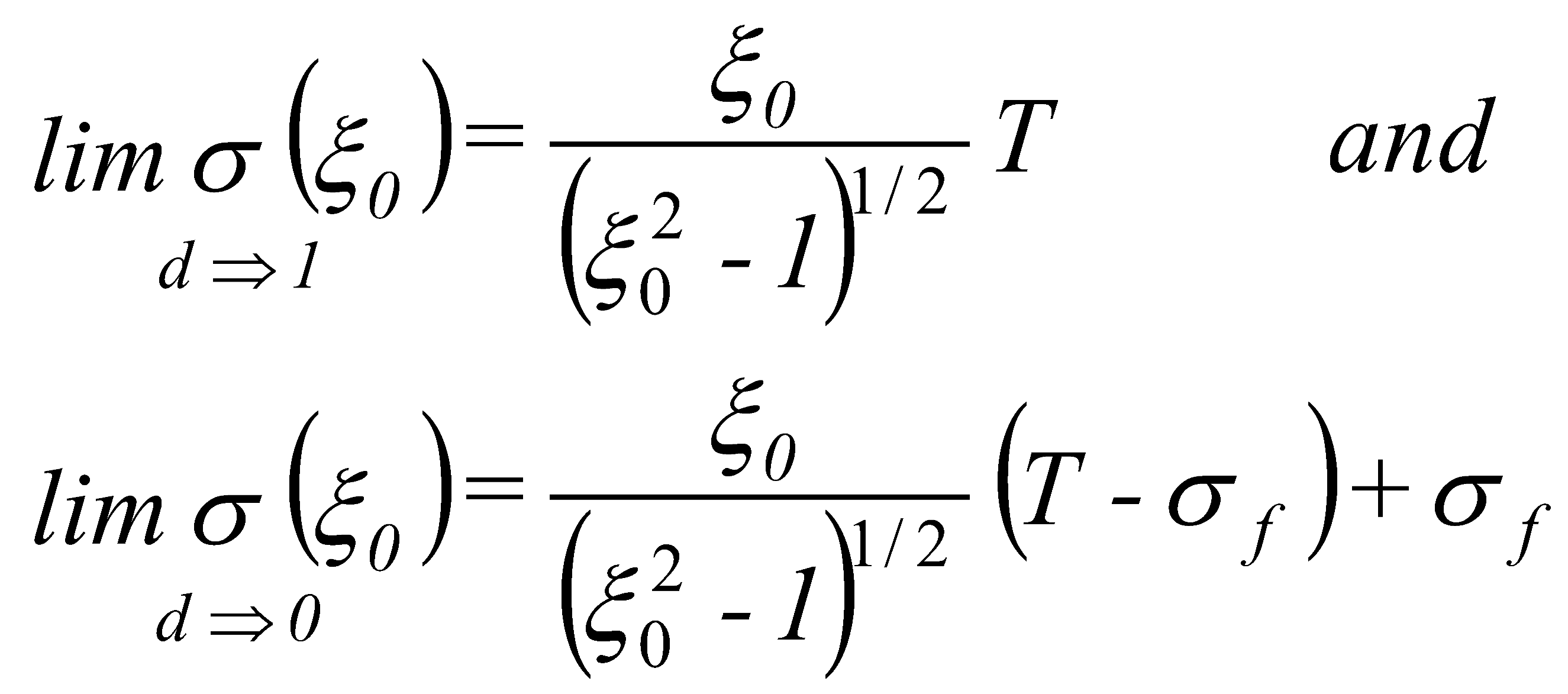 (21)
(21)If we assume that ξo = 1, then:
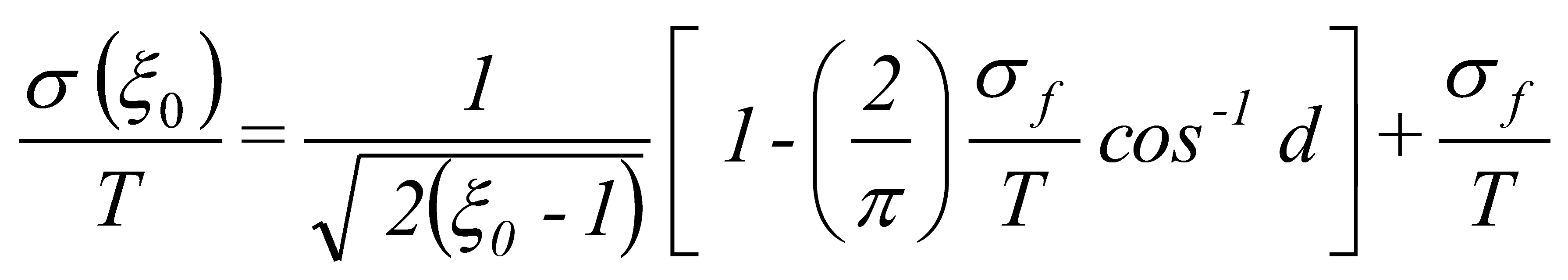 (22)
(22)and we obtain the number of dislocations in the plastic zone by integrating the distribution function between ξ = 1 and ξ = d. The product of the number of dislocations and Burgers vector gives the tooth stress intensity factor Z, a function of plastic displacement. This notation results in [2,3]:
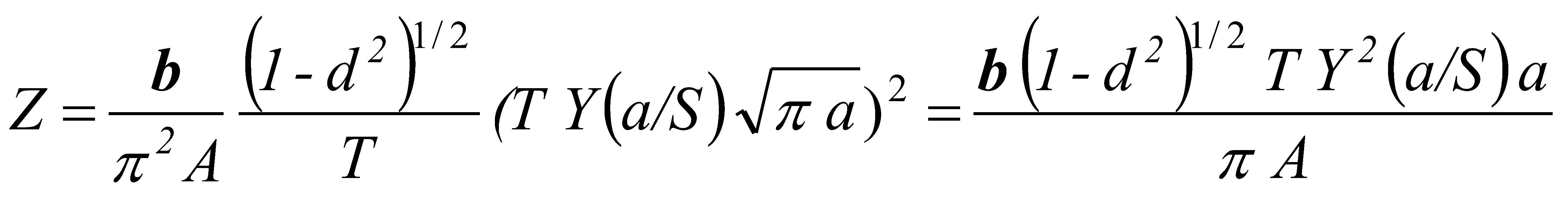 (23)
(23)where the original crack tip location can be simplified as:
 (24)
(24)3.3. Model of Crack Propagation
A great deal has been said and written about crack propagation, so we will repeat it only briefly. Statistical analysis of experimental data reveals that the material parameters in the crack growth equations are random variables. In our code, we used a Paris-Erdogan law to predict the rate of crack growth in materials under cyclic loading and the crack growth ratio [1,2,3]:
and we randomised this equation
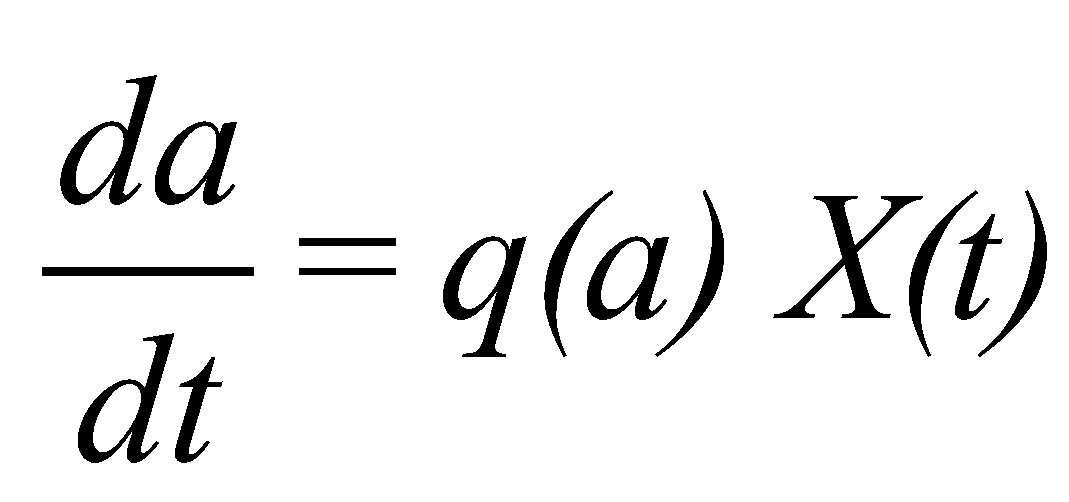 (26)
(26)where X(t) stands for a random process with two extreme scenarios. One scenario is a completely uncorrelated process with only two time points. It might correspond to Gaussian white noise, in which case, the change of time required to obtain the specified crack size would be minimal. On the other hand, the other extreme is a completely correlated process. If we re-examine the crack growth ratio from equation (26) and replace process X (t) with the random variable A, the equation becomes:
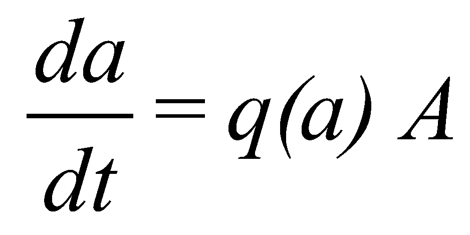 (27)
(27)If integrated with respect to time:
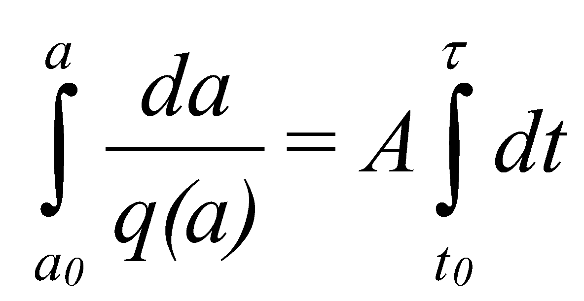 (28)
(28)Where a stands for a(τ). A is transformed in the following manner:
 (29)
(29)By integration of equation (29), the result is:
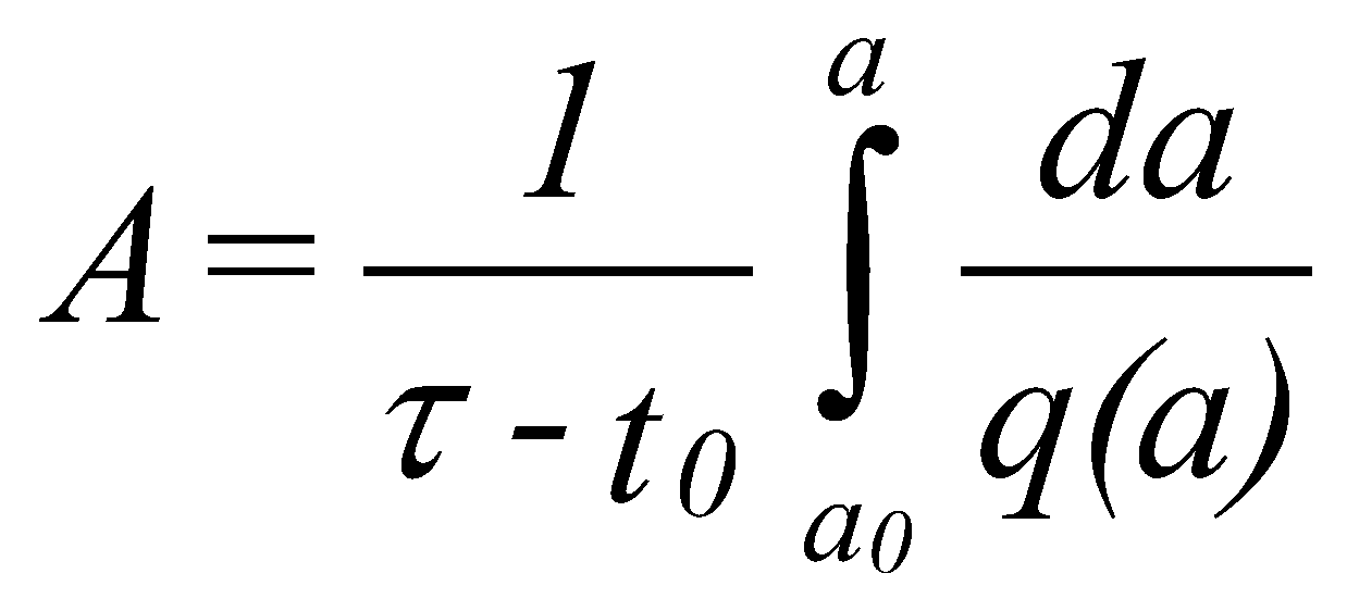
 (30)
(30)Evidently, equations (28) and (30) have identical left-hand sides. Our assumption was that the crack originated within time t in time interval (0,τ), reaching a size of a(t)=a. The crack’s size at the end of the time interval is designated as a(τ), which we obtain by integrating in accordance with equation (30). Clearly, the crack’s size a(τ) is a random variable at a fixed time τ, considering that the right-hand side of the equation is a time integral of a random process.
Finally, after solving the abovementioned mathematical problem, we calculate the conditional probability function using the equation
 (31)
(31)We can calculate the probability function f(u) for crack size a(τ) at timeτ for u>a using the conditional probability density function fa(u|t), and the probability function fτ(t0) from the crack's initiation time. Therefore:
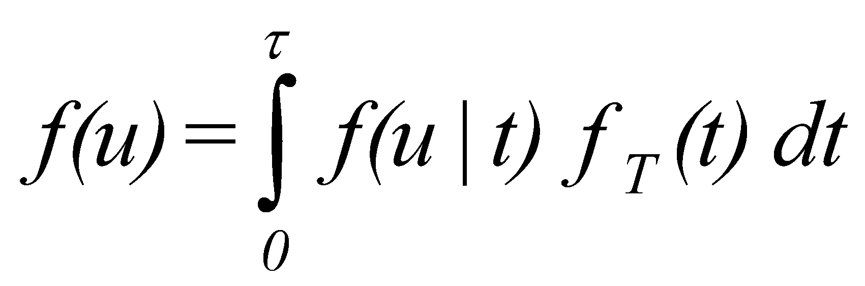 (32)
(32)Integrating equation (32) allows us to determine the distribution of crack sizes for a large number of cracks that are initiated at any time between 0 and τ, following a density of fT(t).
3.4. Experimental Verification of Incubation/Initiation Period
We began the test using three gear test pieces with a number of teeth zpinion = 21. We selected material AISI 4130, which underwent bath nitriding. The tooth width was B = 80 mm, and the profile displacement coefficient was xpinion = 0.8. [1,6], at room temperature and at 50 Hz frequency with the load set as follows: maximum force Fmax = 50,1-50,2 kN, and a ratio R = Fmax/Fmin = 0,1.
3.4.1. Crack Incubation and Initiation
As we did not have a number of different methods available for observing what is happening in the subjects at the level of incubation nor any subsequent initiation of potential methods, we only used the fractografic/metalographic method to confirm the correctness of the model used and to obtain an interpretive model for describing the situation, with which we analyzed the conditions in the material. The entire research was carried out on three species, which were subjected to stress after certain load cycles
- 5 x 10⁴
- 105 and
- 2x10⁵ cycles
we stopped and performed a fractographic analysis on samples from the test subjects.
3.4.2. Fractography
In previous models [1,6], we determined only the consequences, i.e., the final state, and verified the mathematical model with this state. We found the model to be good because it gave us a reliability between 5 and 12%. The model itself, however, did not explain the phenomena that were happening in the material and did not answer the question of why. In contrast, the presented model also allows us to understand the phenomena that occur at the nano and micro levels during the process of nucleation and crack initiation. An explanatory model serves as a helpful tool in describing and explaining why and how something functions or why a particular phenomenon is in its current form. Such explanatory models do not aim to offer a complete description or explanation of the absolute reality of a phenomenon, nor do they aim to be completely accurate. However, what our description/explanation does is that it aligns well enough with a significant portion of knowledge, observations, and theoretical circumstances surrounding crack incubation, which is why such an explanatory model might turn out to be very beneficial.
4.1. Indirect Confirmation for Initiation and Incubation of Cracks
Since we did not have the opportunity to trace the initiation and incubation of the crack in real time, we used the fractographic method to analyze this area. We used three test pieces, which we loaded, as in previous studies, on the Instron hydraulic pulsator. We stopped the test after 5 x 10⁴, 105, and 2x10⁵ cycles. We made appropriate samples for fractographic investigations from each test piece, which were then carried out at the Faculty of Mechanical Engineering, University of Maribor, and at SIJ Metal Ravne, Metallographic Laboratory on optical, quantum, and row electron microscopes with a magnification of up to 180,000x.
- The results of the first fractographic examination of 5 x 10⁴ cycles are shown in Figure 5, where the formation of the initial and the grouping of defects around the initials and dislocations, probably in the form of micro lunkers or similar defects, can be observed.
- Figure 6 and Figure 7 present the results of the second fractographic study after 105 load cycles, and indicate the grouping of different defects, especially in the form of dislocations, and the potential formation of initials for the formation of cracks. Figure 7 thus shows two principles of creating potential cracks: initials that do not expand (crack arrest) and can lead to pitting on the gears, and initials that can lead to the initiation of potential cracks.
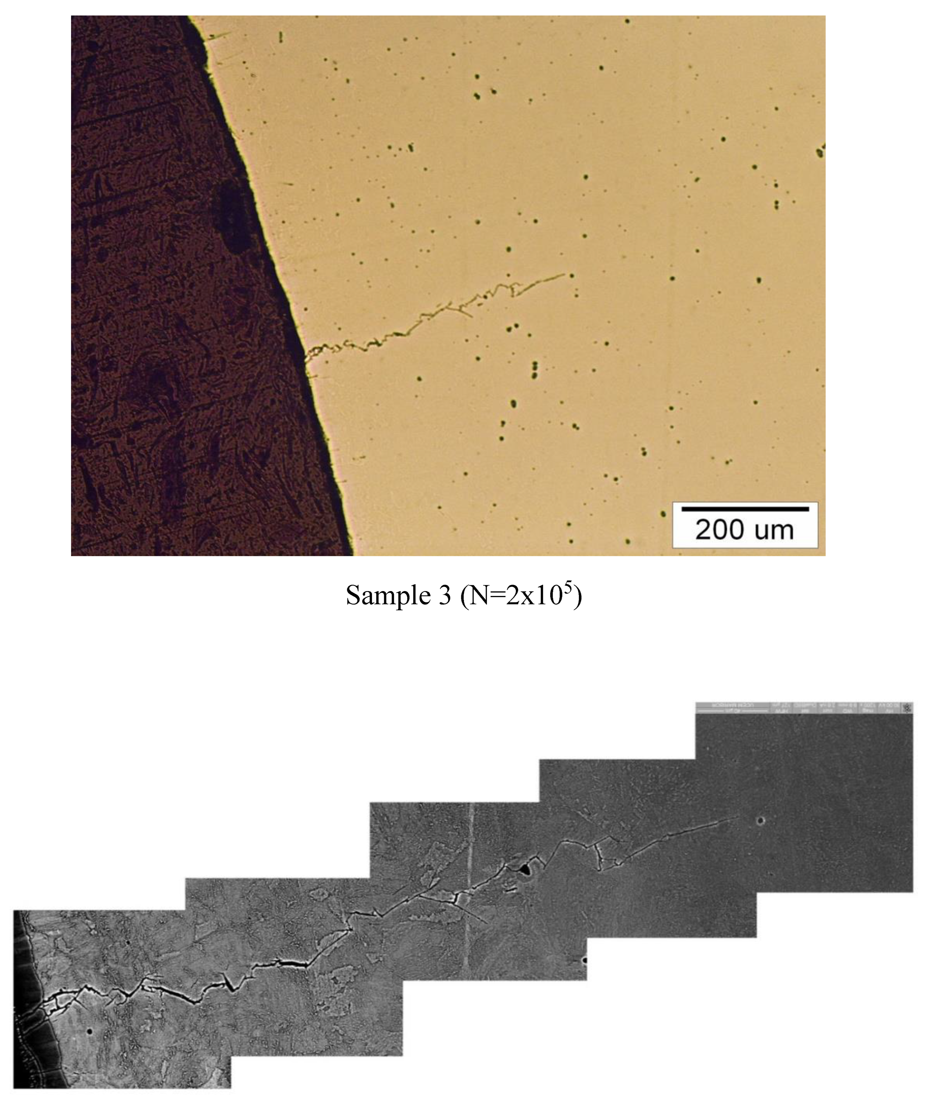
- The results of the third fractographic study after 2x10⁵ load cycles are shown in Figure 8 and Figure 9. Thus, Figure 8 shows the start of the spread of microstructural short cracks, from which it can be observed that the main model of crack propagation is along the boundaries of crystals. Figure 9 shows the entire course of the spread of microstructural and physical short cracks (see Kitagawa-Takahashi diagram - Figure 3), where the crack length is at the limit of detection, and when cracks can be detected by various non-destructive detection methods that have been used in previous studies.
4. Discussion
For the determination of incubation and initialization of cracks, we incorporated the developed code (Equations 1 - 12) into the model used in previous research [1,2]. By doing this, we were able to combine both studies and use the findings of previous research to determine and explain the entire lifespan of a crack and explain the phenomena of incubation and crack initiation, in our case, for cracks in the root of the gear tooth.
To confirm our model’s accuracy for calculating service life, we used two types of explanations, one for the initiation and incubation of the crack, for the area where the strain/stress state cannot be traced in real time with appropriate experimental methods, and the other for the area of crack propagation from micro to macro size for which, however, there are a number of experimental methods.
Based on this, we have developed an appropriate logical argumentation of the explanatory model, based on logical deduction and the umbrella law [19].
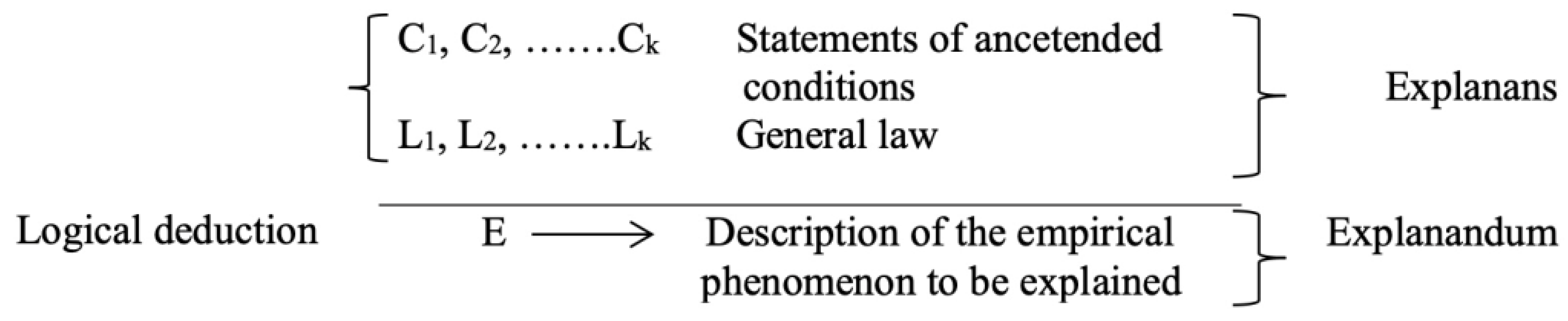
The logical explanation should be divided into its two primary components, the explanandum and the explanans, where the explanandum refers to the phenomenon to be explained (rather than the phenomenon itself), and the explanans refers to the class of sentences that are provided to explain the phenomenon. Two subclassesmake up the explanans; one containing sentences (Ck - eq. 12, eq. 23) with specific antecedent conditions; the other (Lx) representing general laws (eq. 13). For a proposed explanation to be deemed as sound, its components must meet specific conditions of adequacy, which can be grouped into three logical conditions:
- the explanandum must logically follow from the explanans;
- the explanans must refer to general laws, and these must be genuinely necessary for deriving the explanandum, and
- explanans must be supported by empirical content;
and an empirical condition: the sentences making up the explanans must be factual (true).
It is worth noting that the same formal analysis, including the four necessary conditions, applies to both scientific prediction and explanation. The distinction between scientific prediction and explanation is of a pragmatic character. (Hempel, 1970). Following such logical deduction, we physically explained the values of crack incubation from 0-105 and divided it into the formation and cracking of defects (dislocations), which represents the incubation of cracks and the further grouping of defects into the emerging nano cracks, which can be seen in Figure 6 and Figure 7. The further cracking of these nano/micro cracks can be seen in Figure 8 and Figure 9, which were found by fractographic studies after 2x10⁵ cycles. These results were compared with numerical and experimental results of our previous research [1,6].
4.2. Crack Propagation
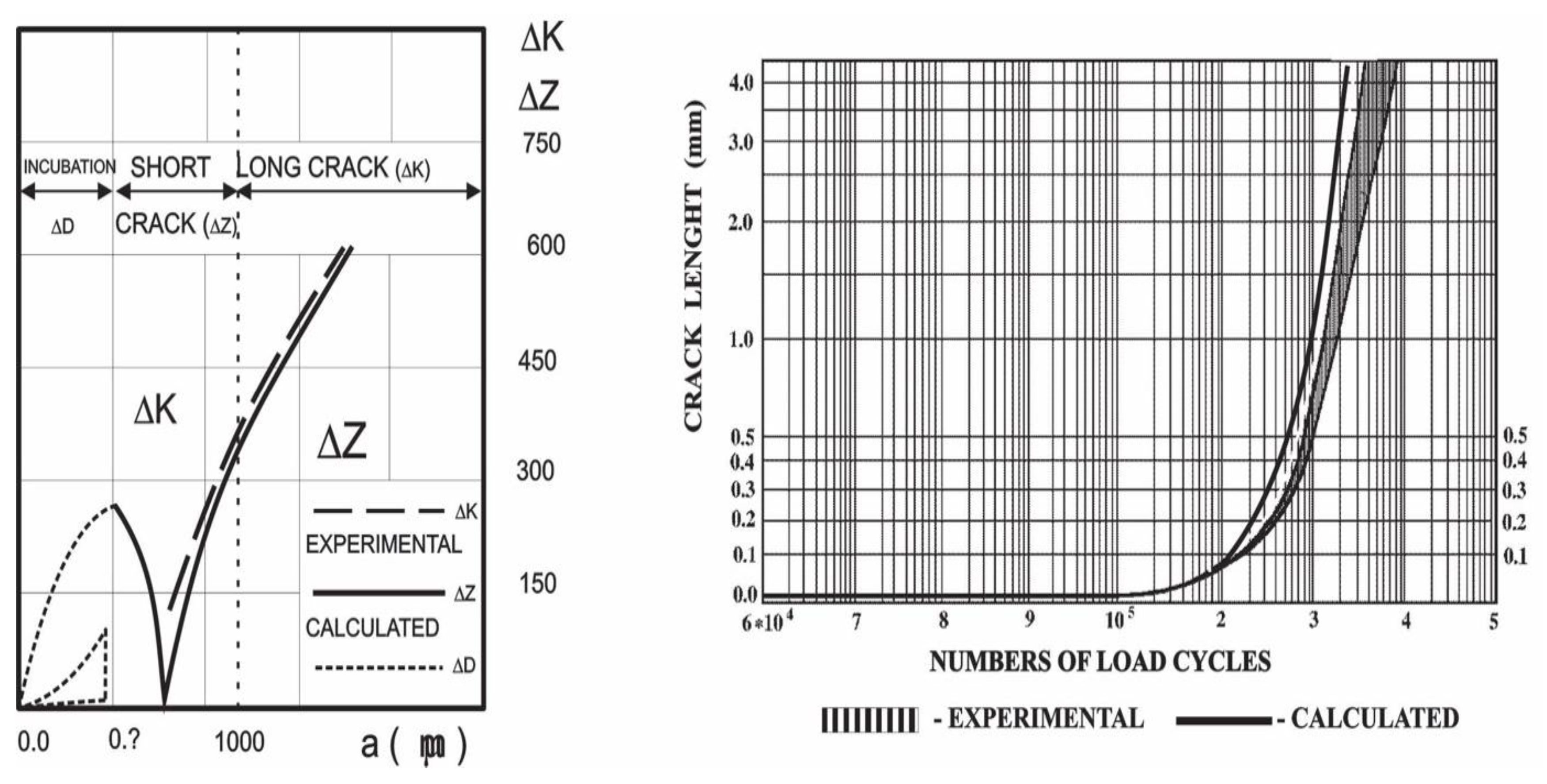
For example, as presented in Figure 10, the critical crack length was approximated at ac≅3.5 mm. Thus, the allowable crack ap = 1.75 mm [9,10]. The deviation increases slightly in the area where we approach the material’s critical length or impact strength. Yet, perhaps most importantly, our model provides reliable results since the final collapse of the structure in the critical area does not yet occur in the calculations. In practice, in deterministic calculations, we always introduce a safety factor, so that we never allow the collapse of the structure to occur (the crack reaches a critical length). Based on this, using deterministic methods from various standards is insufficient for precise calculations of the service life of the structure. Thus, we developed a gear loading intensity factor Z (eq. 23) for the calculations. The factor accounts not only for the stress in a homogeneous material in the critical cross-section but also for stress concentration due to errors present within that section. Using the Z factor, we have created a generalized model that, in addition to crack propagation, also includes incubation, initiation, and crack growth, with the help of which the actual service life can be calculated more accurately. With the model presented, we even achieved a slightly lower deviation compared to previous models [1,2], achieving a deviation of just 5 to 10% from experimental results, which is considered highly accurate for such calculations.
Let us devote a little more space to the explanation of incubation and crack initiation, since the propagation model is described in our previous research [1,2], and we have only briefly summarized and repeated the explanations here. The results, shown in Figure 10, show a comparison between the data obtained experimentally and the values calculated using the suggested mathematical models. Based on experiments and using standard methods (general law, eq. 13 and 25), we establish diagram ΔK - a and compare it to a similarly calculated diagram, i.e., ΔZ/D - a (explanandum, eq. 12 and 23). Based on this, we calculated the gears’ service life to be approximately 3.3x10⁵ load cycles. If we compare this with the experimental data of 3.5 - 3.8 x 10⁵, we can conclude that the deviation is more acceptable. However, it is also important that, using the presented model, we get a calculation that is always on the safe side. Not only did we get a model that gave us good results, but we also got an explanatory model that explained what was going on in an area where it was almost impossible to determine the conditions of incubation and early crack initiation. In the classical, deterministic approach, we can say that we have achieved a safety factor of 1.05 - 1.12, which is an extremely low safety factor for dynamical systems (usually greater than 2).
5. Conclusions
Education is currently undergoing major changes from its traditional approach, which still places the student in a passive learning position. Today's progressive learning environment is seeing a rise in popular phrases such as outcome-based teaching methods based on non-formal distance learning, teamwork, and AI [5]. The effectiveness of these changes indicates the need for a large-scale reconceptualization and transformation of the learning process. Achieving this will require teachers to engage the students as independent and active learners. We will need to provide powerful new technologies to establish an information-rich and intelligent learning environment, where students and teachers will be able to navigate the various informational superhighways [5]. One such option is presented in this paper. It is important that we have not only provided students with an optimization model for the construction of gears, but also provided an explanatory model that explains what is happening in an area where it is almost impossible to determine the conditions of incubation and early initialization of cracks. We have given the students the knowledge with which they will be able to critically develop and optimize appropriate solutions.
Funding
This research received no external funding.
Institutional Review Board Statement
“Not applicable”.
Conflicts of Interest
“The authors declare no conflicts of interest.”
References
- Aberšek, B.; Flašker, J. How gears break, WIT Press: UK, 2004.
- Aberšek, B.; Flašker, J. Numerical methods for evaluation of service life of gear, International Journal for Numerical Methods in Engineering,1995; Vol. 38, 2531-2545.
- B. Aberšek, J. Flašker, J.; Glodež, S. Review of mathematical and experimental models for determination of service life of gears. Eng. fract. mech. 2004, vol. 71, iss. 4/6, 439-453.
- Buehler, M.J. , et al., The Computational materials Design Facility (CMDF): A powerful framework for multiparadigm multi-scale simulations. Mat. Res. Soc. Proceedings, 2006. 894: p. LL3.
- Flogie, A.; Aberšek, B. Artificial intelligence in education. IN: LUTSENKO, Olena (ur.). Active learning - theory and practice. London: IntechOpen, 2022, 97-117. [CrossRef]
- Aberšek, B.; Flašker, J. Experimental Analysis of Propagation of Fatigue Crack on Gears, Experimental Mechanics, 1998, Vol. 38, No. 3, 226-230.
- J. W. Provan, W. Probabilistic Fracture Mechanics and Reliability, Martinus Nijhoff Publishers, Dordrecht, Boston, Lancaster, 1987.
- Spergel, D.N. , Turok, N.G., Textures and cosmic structure, Sci. Am., 1996. 266: p 52-59.
- Zurek, W.H. Cosmological experiments in condensed matter. Phys. Rep., 1984. 276 : p 177-221.
- Bradač, Z. , Kralj, S., Žumer, S., Early stage domain coarsening of the isotropic-nematic phase transition, J.Chem.Phys., 2011. 135 : p 024506-024516.
- Imry, Y.; Ma, S. , Random-Field Instability of the Ordered State of Continuous Symmetry, Phys. Rev. Lett., 1975. 35 : p 1399-1402.
- Aharony, A.; Pytte, E. , Infinite Susceptibility Phase in Random Uniaxial Anisotropy Magnets, Phys. Rev. Lett., 1980. 45: 1583-1587.
- Bellini, T.; et al. Nematics with quenched disorder: What is left when long range is disrupted? Phys. Rev. Lett., 2000. 31: 1008-1011.
- Mermin, N.D. , The topological theory of defects in ordered media, Rev. Mod. Phys., 1976. 51: 591-648.
- Lubensky, T.C.; Renn, S.R. , Twist-grain-boundary phases near the nematic–smectic-A–smectic-C point in liquid crystals, Phys. Rev.. A, 1990. 41. p: 4392–4401.
- Abrikosov, A.A. On the Magnetic Properties of Superconductors of the Second Group, Soviet Physics JETP, 1957. 5: 1174-1182.
- De Gennes, P.G. , Prost, The Physics of Liquid Crystals (Oxford: Oxford University Press), 1993.
- Taylor, D. ; J. F. Knott, J.F. Fatigue crack propagation behaviour of short crack; the effect of microstructure, Fatigue Engn. Mater. Struct., 1981 4, 147 - 155.
- Hempel, C.G. Aspects of Scientific Explanation and Other Essays in the Philosophy of Science. New York: The Free Press, 1965.
Figure 1.
A schematic view of a complex Knowledge-Based ES.
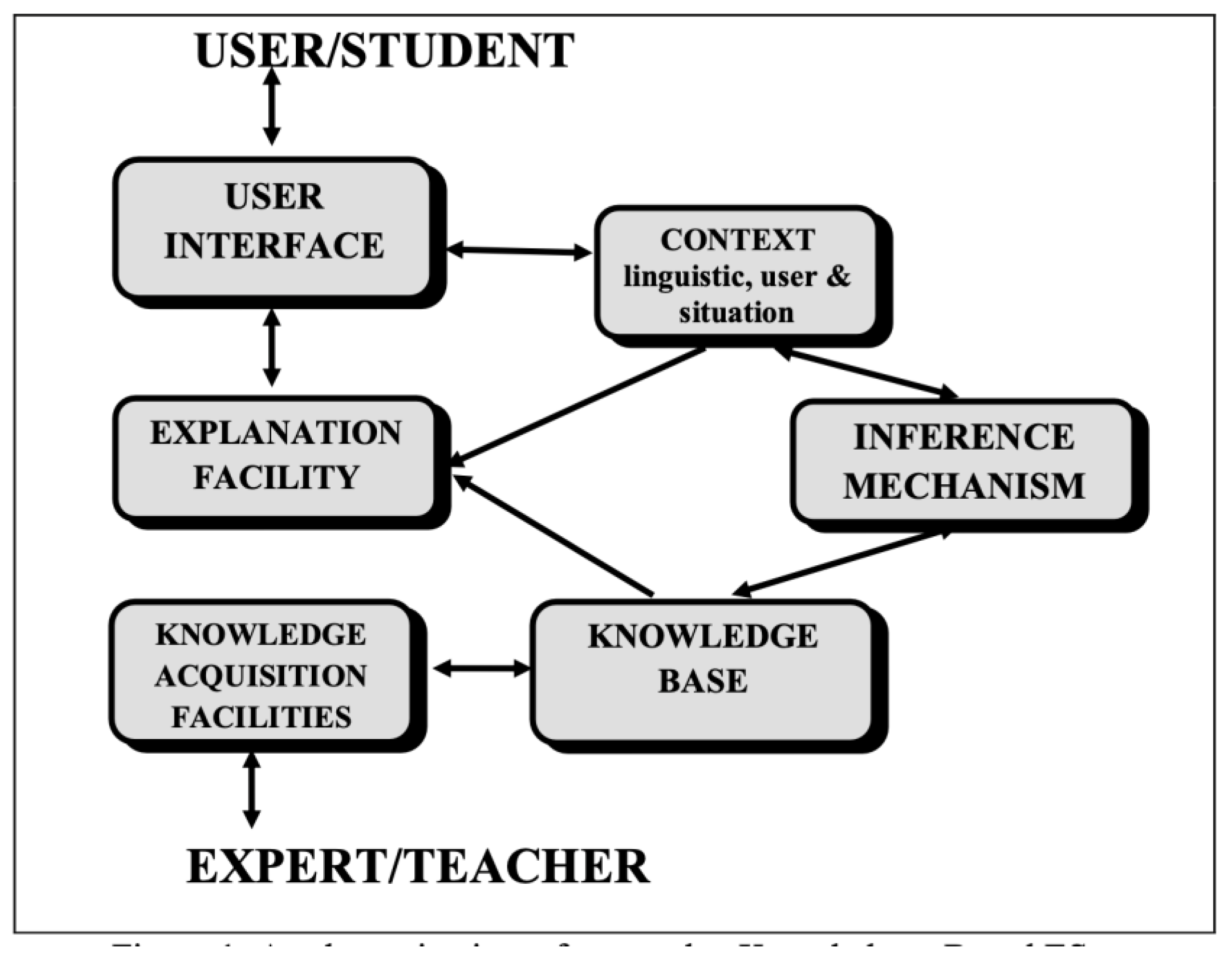
Figure 2.
Configuration of our expert system [1].
Figure 2.
Configuration of our expert system [1].
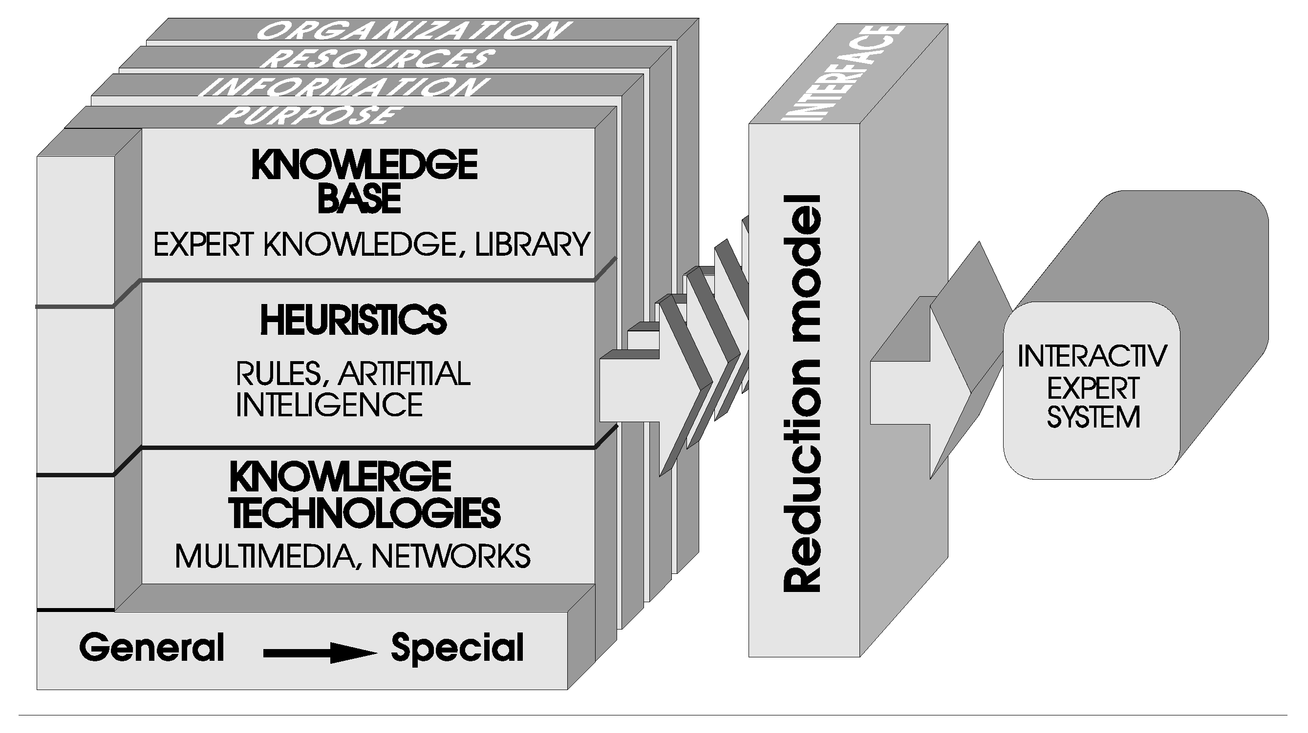
Figure 3.
Kitagawa-Takahashi diagram - Crack properties regimes.
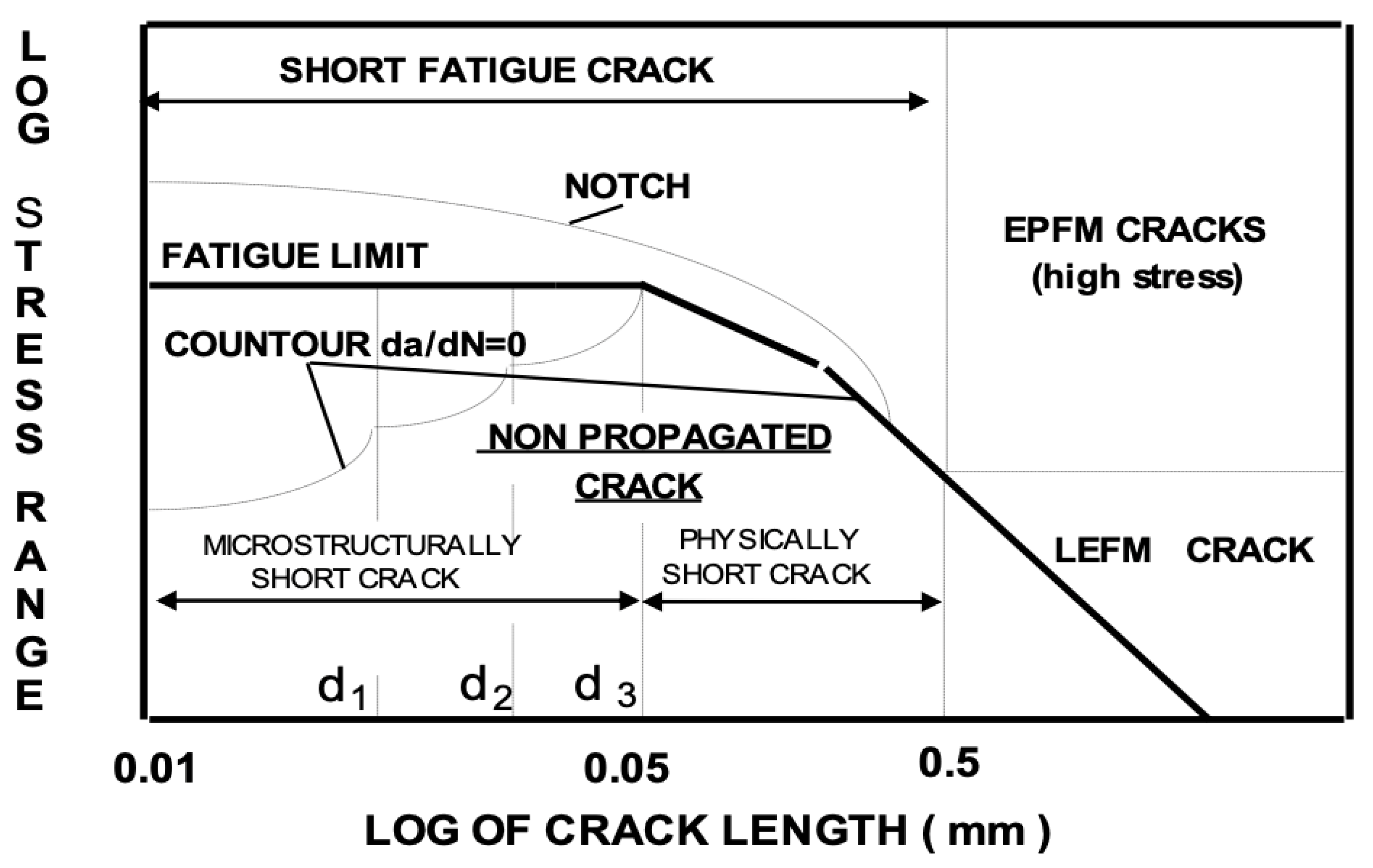
Figure 4.
Edge dislocation (a) and spiral dislocation (b).
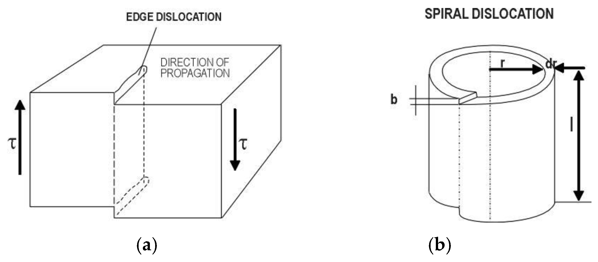
Figure 5.
Sample 1 after 5x10⁴.
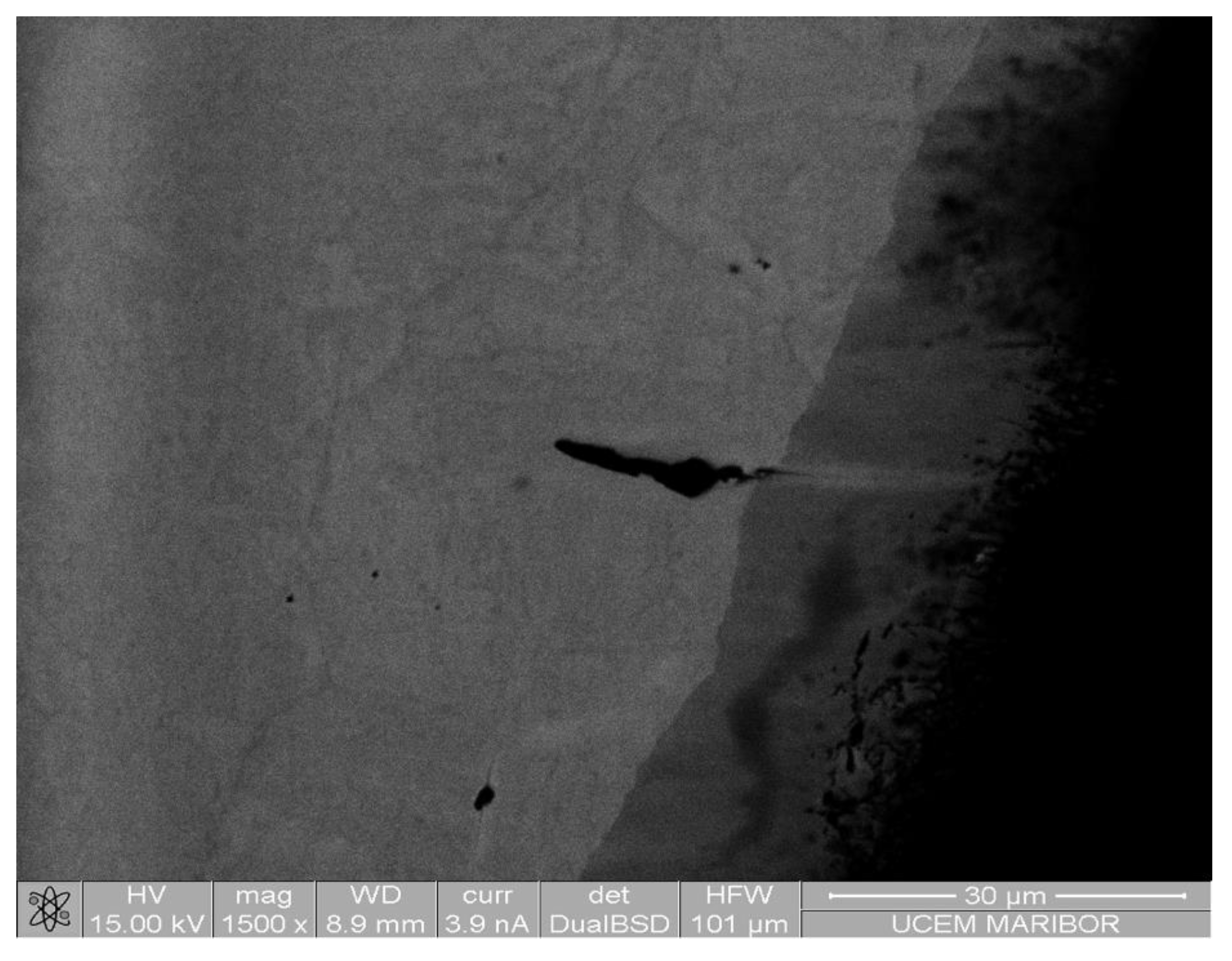
Figure 6.
Sample 2 after 105.
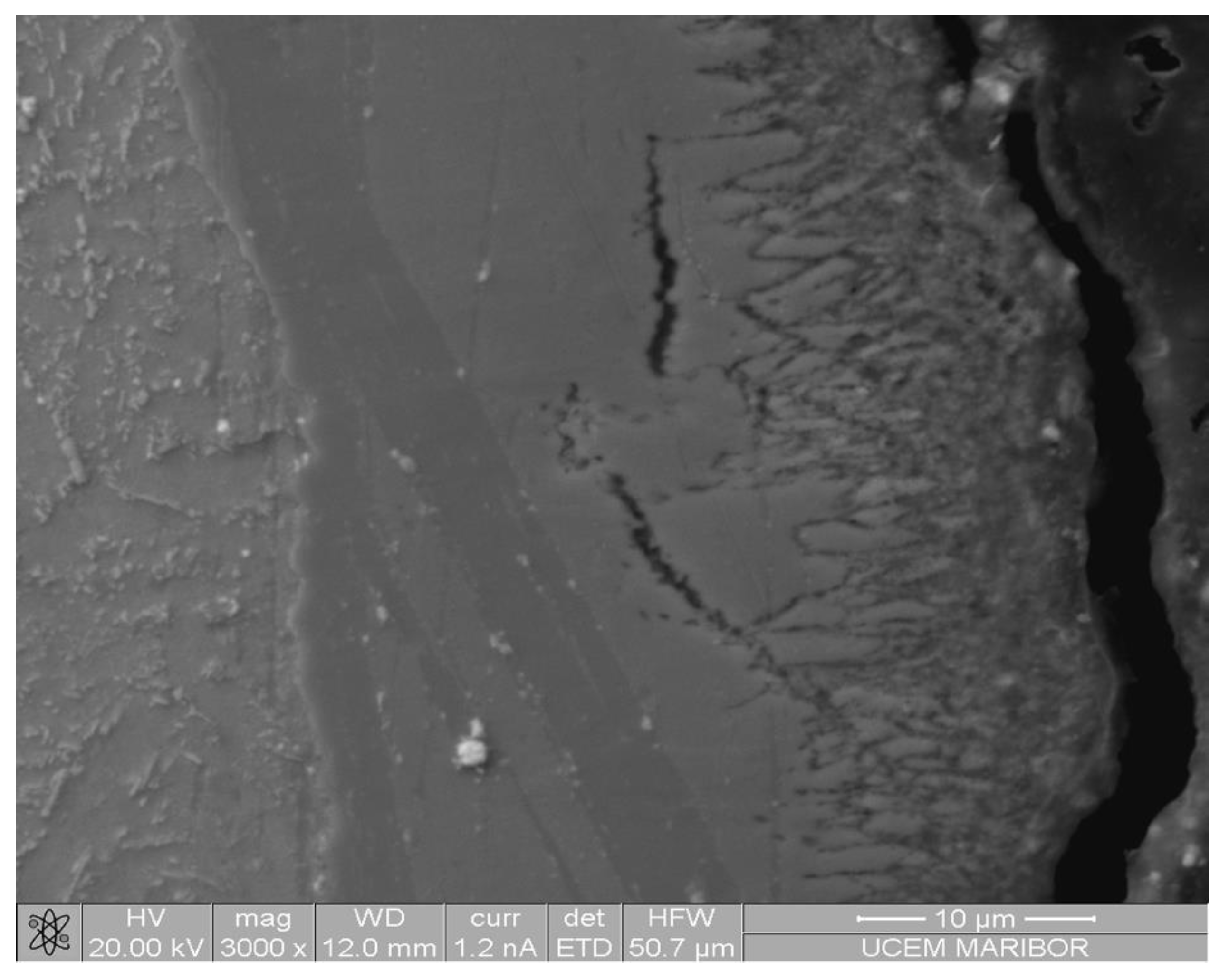
Figure 7.
Sample 2 after 105.
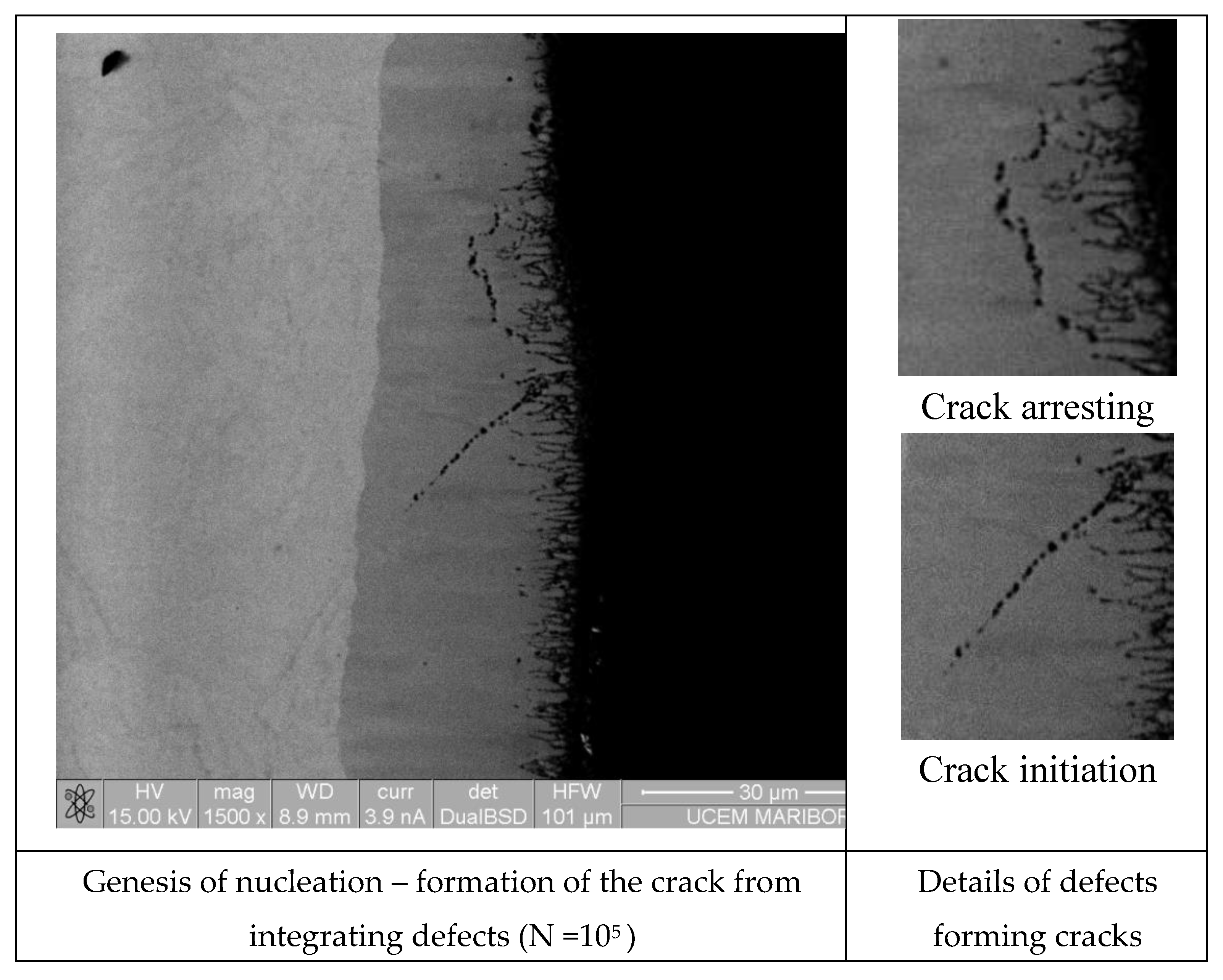
Figure 8.
Sample 3 after 2x10⁵ Initiation and propagation of short crack - formation of microstructural and physical short crack (see Kitagawa-Takahashi diagram - Figure 3).
Figure 8.
Sample 3 after 2x10⁵ Initiation and propagation of short crack - formation of microstructural and physical short crack (see Kitagawa-Takahashi diagram - Figure 3).
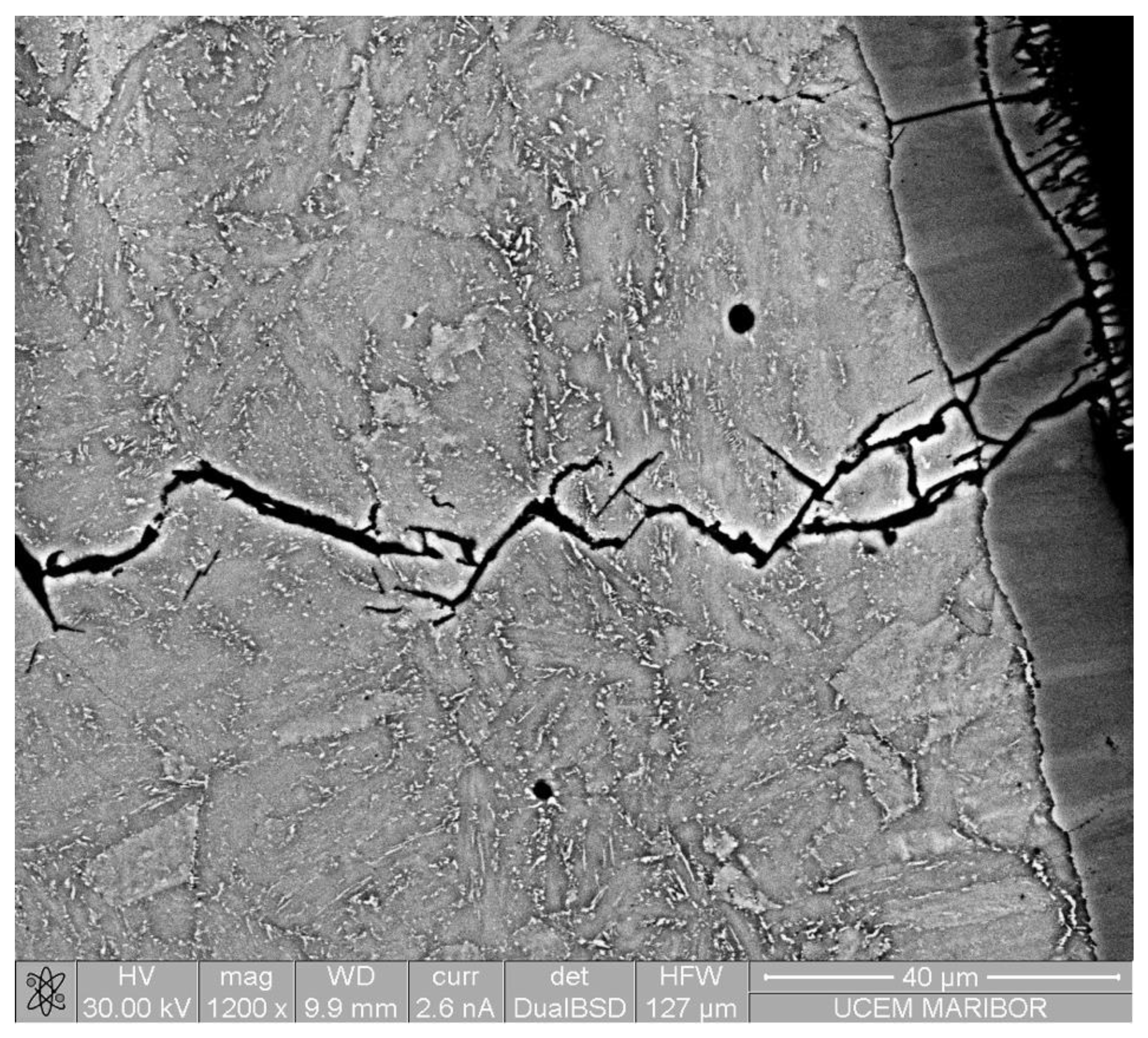
Figure 9.
Genesis of micro cracks growth (Approx. 500 microns long, approx. N= 2x 10⁵).
Disclaimer/Publisher’s Note: The statements, opinions and data contained in all publications are solely those of the individual author(s) and contributor(s) and not of MDPI and/or the editor(s). MDPI and/or the editor(s) disclaim responsibility for any injury to people or property resulting from any ideas, methods, instructions or products referred to in the content. |
© 2025 by the authors. Licensee MDPI, Basel, Switzerland. This article is an open access article distributed under the terms and conditions of the Creative Commons Attribution (CC BY) license (http://creativecommons.org/licenses/by/4.0/).
Copyright: This open access article is published under a Creative Commons CC BY 4.0 license, which permit the free download, distribution, and reuse, provided that the author and preprint are cited in any reuse.


