

Submitted:
04 July 2025
Posted:
07 July 2025
You are already at the latest version
Abstract
The main idea behind this research was to build a unique algorithm from scratch, by combining different pre-existing methods, capable of detecting a person in the wild nature. The challenges to overcome are small object detection and lack of computing power. The inspiration for detection in wild nature environment came with a cause to create an algorithm, capable of learning patterns and features of an object, without labeled data. The algorithm developed (SARGAS) utilizes custom convolutional neural network classifier as main detection tool in combination with MOG2 background subtractor and partial affine transformations for camera image stabilization purposes, with a secondary binary classifier for detection re-assurance. Results have far exceeded the initial expectations, a solid ground for future development and improvements has been set as 93% recall result has been achieved, with a total accuracy of 65%. The proposed method currently is inferior to under supervision trained algorithms like YOLO, when the setup is similar to training data, but we strongly believe that unsupervised CNN algorithms can outperform the supervised models. The proposed method holds great potential within it, but has to be refined further.
Keywords:
object detection
; background subtraction
; neural network
; computer vision
; target tracking
; search and rescue
; unsupervised
; machine learning
; dataset
; classification
1. Introduction
A large number of people go missing every year in the wilderness or perish due to natural disasters. The failure to provide timely assistance is a frequent cause of death, however, even more frequently, the rescuer ends up in a victim position, due to excessive self-confidence and hastiness [1]. To locate missing persons and those affected by disasters, search and rescue operations are conducted. A “search” is a systematic operation using available personnel and resources with the goal of finding people who have encountered a disaster. A “rescue” is the operation of extracting those affected by a disaster and bringing them to a safe place.
One of the world's first search and rescue missions was conducted in 1656 when the Dutch merchant ship Vergulde Draack wrecked on the western coast of Australia [2].
Search and rescue teams are constantly striving to improve their operations by developing new ways to quickly find a lost person. Search and rescue missions are divided into several types, such as mountain rescue, ground search and rescue, urban search and rescue, air and sea rescue, and combat search. The process is just as dangerous for the rescuer as it is for the victim.
In search of a missing person, every second matters, however, utilizing drones and the newest technologies it is now possible to search vast areas in a short time span as well as places, that are hard to reach, therefore increasing the rate of survivability, while decreasing search time. There are numerous object detection algorithms, however, only a small amount of such algorithms can be used for search and rescue missions. The currently existing methods are unreliable, foreign objects are often recognized as objects of interest over the actual object of interest. The accuracy of such algorithms is usually determined by the quality of training.
One of the studies examined the effectiveness of drones in search and rescue operations in the mountains, searching for lost people [3]. Two teams were formed for the study: the first team consisted of five professional certified rescuers, and the second team consisted of three rescuers with snowmobiles and one certified drone pilot. The first team performed the search and rescue mission on foot, following the guidelines of the traditional method. The second team used a drone for the search, and when a lost person is found, a team of three rescuers with snowmobiles is dispatched to retrieve the lost person. The efficiency indicators of the method in the article were the detection time and the searched area. The first team, over 10 tests, detected a person on average in 3779 seconds and searched an area of 90996 square meters, while the second team's average detection time was 531 seconds, and the average searched area was as much as 233876 square meters. The results show the obvious advantage of using a drone in life-threatening situations. In a shorter period, a 2.57 times larger area of the territory is searched, and 54 minutes are saved.
In another paper [4], the authors propose using a drone as an auxiliary tool in search and rescue missions to assess earthquake damage to infrastructure using cameras and thermal imaging cameras integrated into drones. According to the author, obtaining information about infrastructure damage after an earthquake is very important for the rescue process and loss assessment. It often happens that when rescuing people from under the rubble, the remaining infrastructure collapses, and then the rescuers themselves have to be rescued. Using infrared thermal imaging technology to automatically detect structural damage to buildings and cracks in external walls, it is possible to quickly assess the risk, thereby reducing the number of further victims. In the article, the overall accuracy of the method ranges from 81 to 88 percent. The confusion matrix obtained by calculating real pixels on the ground surface and the corresponding pixels in the classification results was used for the evaluation.
Another important reason for automating the search and rescue process is the human factor. Statistically, 60-90 percent of all accidents are caused by human error [5], [6], [7]. In order to reduce the probability of human error and speed up the reaction time, scientists from various fields are studying image recognition algorithms, their applications, and automation possibilities. Today, image recognition is used in medicine [8], [9], self-driving cars [10], electrical wiring defect detection [11], construction industry [12], agriculture [13], road engineering [14]. Thanks to these and many other scientific works, a trend has emerged to use high-performance image processing-based methods, such as machine learning and deep learning methods, which allow processing huge amounts of data more simply and efficiently.
Machine learning has been discussed by many researchers. Tom Mitchell defined machine learning as the study of computer algorithms that automatically improve through experience [15]. Ethem Alpaydin considered that “machine learning is the programming of computers to optimize performance criteria using sample data or past experience” [16]. As early as 1958, Herbert Simon stated that “the world now contains machines that think, learn, and create. Moreover, their ability to do these things will increase rapidly until, in the foreseeable future, the range of problems they can solve will match human mental abilities.” [17]. The general prevailing view of machine learning is that computers gradually develop by improving their intellectual abilities by imitating human behavior. However, unlike humans, computers do not get tired, get distracted, or make human-like errors.
Machine learning can be roughly divided into two categories, supervised and unsupervised learning, depending on whether the training data is labeled [18]. In supervised learning, an algorithm learns from an example of labeled training data in order to be able to independently label new data. Unsupervised learning uncovers key features and patterns from unlabeled training data.
Currently, the convolutional neural network (CNN) is one of the popular object detection methods. As time passed by, the need for the use of larger datasets has arisen, and technological advances have provided opportunities to meet these needs. In 2012, the deep learning network AlexNet proposed by A. Krizhevsky [19] became the winner of the ImageNet Large Scale Visual Recognition Challenge (ILSVRC) competition. The presented model became a sensation that shook the AI industry. AlexNet had a 10.9% lower error rate than the second-place model. Since then, AlexNet has been considered the pioneer of deep learning, and much more advanced and accurate algorithms have emerged after it, including VGG [20], LSTM [21] , and ResNet [22]. These models are widely used in image recognition, speech recognition, translation, etc.
In a brief introduction to convolutional neural networks (CNN), let us discuss the widely used CNN VGG16 as an example to introduce the components of a CNN [23]. The most important part of a convolutional neural network is the convolutional layer. Each convolutional layer has a certain set of convolution kernels, which are responsible for extracting specific features from the input. The output or set of extracted features is also called a feature map. The input and output are usually of the same size, and a pooling layer is used to reduce the size of the feature map. For example, our input is a 224x224 RGB image, after applying our convolutional layer we get 64 224x224 outputs or 64 feature maps of size 224x224. Thus, our output represents 64 different pixels that were detected by 64 different convolution kernels. By applying a pooling layer, we reduce the resulting feature maps to 112x112, then apply a convolutional layer again, a pooling layer, and the process is repeated until we get a 7x7 output. It is important to note that each time we apply a convolutional layer, the number of detected objects also increases.
Typically, algorithms can be divided into two categories: one-stage and two-stage algorithms. The most well-known two-stage algorithms are the R-CNN series of algorithms: R-CNN [24], Fast R-CNN [25], and Faster R-CNN [26]. Examples of one-stage algorithms include the „YOLO“ series or the „SSD“ algorithms [27], [28].
You Only Look Once (YOLO) pioneered single-stage detection algorithms that combine object classification and localization in a single neural network. Single Shot Detector (SSD) is another single-stage detection algorithm based on YOLO, borrowing the anchor box idea from Faster R-CNN and emphasizing the extraction of multiple feature maps [29].
Researchers in various fields are modifying and refining existing algorithms, continuously improving accuracy. In China, scientists adapted and improved the Yolov7 algorithm for human search and rescue purposes in open water conditions, improving detection accuracy from 87.1 to 91.6% [30]. A different study was conducted to improve the accuracy of human detection in search and rescue operations in winter conditions by changing the input image resolution. Using higher-resolution images results in more accurate detection results, but in return, the detection time indicator deteriorates. According to the author, at a resolution of 224x224, the detection accuracy ranges from 34 to 94 percent accuracy, and at a resolution of 3840x2160, the accuracy is 70-94 percent [31]. In another paper [32], a new algorithm is developed based on the mean shift algorithm to apply it to search and rescue operations in the mountains. The original mean shift algorithm showed a result of 74.7% recall and 18.7% precision, while the newly developed CNN showed a result of 88.9% recall and 34.8% precision. Despite the fact that the result has improved significantly compared to the original algorithm in general, the final accuracy is relatively poor. Another drawback of this algorithm is that the processing of 40-50 photos, including human detection, took 1110 s, which emphasizes the relevance of our study. A common flaw of these works is that the training material is very similar to the material provided to the algorithm during testing. Such tests achieve a good accuracy rate but do not show the real accuracy of the algorithm in realistic circumstances. In the first work, the algorithm shows good accuracy in calm waves, however, most accidents occur in adverse weather conditions. The second work under consideration showed unstable results, the accuracy deteriorates when snow is not present, or foreign objects such as trees appear in the frame. The third work under consideration shows the most realistic result, but due to its detection time, it is unsuitable for search and rescue missions, where every second counts.
In this scientific work, the aim is to create an algorithm capable of detecting a person in the wild, based on footage from a drone or unmanned aerial vehicle. Conventional CNNs are highly accurate in performing stationary object recognition tasks, but face difficulties in detecting moving objects. To solve this problem, we propose to integrate a motion detection method into the CNN. Today, motion detection methods include improvements to the original methods, such as the frame difference method [33], the background subtraction method [34], [35], the Horn-Schunk [36], and Lucas Kanade [37] optical flow methods. It is likely that even after successfully combining CNN with the motion detection method, we will encounter a typical issue that comes along with motion detecting methods – the motion of camera itself, which we will try to solve by applying camera motion suppression methods. The experimental conditions and the methods used are discussed in more detail in the second section of the work.
2. Materials and Methods
In this section, the experimental conditions and methods will be discussed in more depth along with the challenges we had to overcome. The primary objective of this project was to develop a novel algorithm from scratch by combining various existing methods. The purpose of the algorithm in development is to detect small objects from drone footage or unmanned aerial vehicles. In the field of computer vision, the detection of small objects has long been considered a challenging task that scientists have yet to overcome. When compared to large-scale objects, small objects are bound to a limited pixel footprint, which results in reduced features available for extraction during the training phase, leading to an exponential increase in difficulty for models in making accurate object detection or classification predictions. To make things worse, small objects tend to blend with the background and other objects due to similarity in shape, color, or texture, causing false positives and false negatives.
Furthermore, algorithms are prone to overfitting or underfitting when it comes to training for small object detection tasks. A best-fitting set of hyperparameters for CNN must be determined, such as the number of layers, filters, iterations, etc. To overcome this challenge, a method of trial and error was used. Another possible issue is computing power. CNNs inherently require significant computational resources, and our approach incorporates not only multiple CNNs but also motion detection methods, which further intensify the computational load and strain on hardware resources.
To provide clarity on the development process, a step-by-step breakdown of the algorithm creation and the rationale behind key decisions will be presented in the following sections.
2.1. Dataset and Scenery
The dataset is a crucial part of the project. In order to achieve reliable results, a well-balanced dataset is essential. For this study, the WiSARD dataset was initially used for training purposes [38]. WiSARD visual and thermal images were acquired by a drone across a variety of wildlife environments over an extended period, at varying angles and under different lighting conditions. The dataset consists of three main subsets: a set of 26,862 labeled RGB images called “Visual Only”, a set of 29,989 2D infrared (thermal) images labeled “Thermal Only”, and a combined set of 15,453 synchronized visual and thermal image pairs called “Visual and Timed”.
To improve dataset diversity and better simulate the project’s specific conditions, the WiSARD dataset was later mixed with the author's own filmed footage. This additional footage was captured using a DJI Mavic 2 Enterprise Dual, which is equipped with both thermal and RGB cameras. A lower resolution of 1920×1080 for RGB and 640×360 for thermal images was selected to reduce processing time and enable faster algorithm execution. The drone’s ability to capture time-synchronized RGB and thermal images made it particularly suitable for this study, aligning well with the structure of the WiSARD dataset.
The footage was recorded during winter in a location where human subjects blended easily with the background and with other objects resembling the shape of a human when viewed from above. This scenario presented a challenging test case for the algorithm. During the testing phase, multiple false positives were observed due to the limited size and variation of the winter dataset, particularly the lack of diverse negative samples. Most negative samples consisted of either snow-covered terrain or heavily snow-laden trees. To address this, a portion of the recorded video footage was removed from the test and evaluation set, segmented into frames, and manually labeled for use in training and validation.
Ultimately, the final dataset was formed by merging the WiSARD dataset and the author’s footage in equal proportion, resulting in a balanced 1:1 ratio that improved model generalization and performance across varied environmental conditions.
2.2. Data Preprocessing
Getting the dataset in order was just the beginning. During the training phase, it turned out, that the computing power for our heavy dataset with large-scale images was not enough. Furthermore, when attempting to train on a fraction of the dataset in small batches and perform test runs, based on the evaluation of the test results, it was concluded, that our model is not properly learning. In multiple cases the object of interest occupies only a tiny fraction of the image, as a result, the model ends up learning features from the background or contextual elements that correlate with the object’s presence, rather than focusing solely on the actual object, it was concluded, that computing power alone will not solve the issue and a different approach is needed. Instead of supervised training with labeled samples, we proceeded with the unsupervised training method, where the model is provided with multiple positive and negative cropped samples. The method proved to be more efficient as it required less computational power, was less time-consuming, and provided a significant increase in accuracy. The initial time of training on full-scale images was close to 6 hours and required computing power equivalent to Amazon’s g4dn.8xlarge instance with 32vCPUs, but dropped to just 15 minutes where „g4dn.xlarge“ instance with 4vCPUs is more than enough.
A Python script was written to fully automate the process of sample cropping, by utilizing the existing image labels. The aforementioned „WiSARD“ dataset is labeled in normalized coordinates format, similar to the format that the YOLO algorithm uses, and the hand-labeled images were labeled similarly for convenience. The dataset is divided into negative and positive cropped samples resized to 128x128 each so that the algorithm can learn to understand where the person is. Dividing it into negative and positive samples means that the algorithm will be supplied with two sets of images in equal parts – a positive set and a negative set. The positive samples are image crops containing the object of interest, and the negative samples are images without the object of interest. The total count of samples is 50000, with a perfect split of 25000 for both, positive and negative samples. To further simplify the model training and highlight the unique human-like shape in images, a decision has been made to further preprocess the images by converting samples into grayscale and applying canny edge detection. While grayscale simplifies the image data to a single intensity channel, making it easier to detect intensity gradients without the distraction of color, the Canny edge algorithm computes intensity gradients to identify object boundaries. Both of these features are later fused into a single-layer image by filling the blue and green layers with grayscale image information and the red layer with canny edge information and converting the 3 combined layers back to grayscale, resulting in a final image that blends the original intensity values with the strong edges highlighted from the Canny operation. After preprocessing is finished, the dataset is randomly shuffled five times. After every shuffle, the dataset is split into training and validation sets with a 4:1 ratio and then samples are copied into a separate folder, before repeating the process for a total of 5 times.
2.3. CNN
The first step towards creating the algorithm is to build a custom CNN model. The CNNs are usually used for object detection or classification tasks. When a classification algorithm is given an image, it simply gives us a probability score for each of the classes it is trained to identify. In binary classification, it classifies an image as either positive or negative, depending on the set threshold value. It is possible to split the image into multiple cells, by dividing the image into 9 cells (3x3), and then the algorithm examines each of the cells separately, highlighting the cell or cells which, according to the algorithm, can be classified as an object of interest, with a probability exceeding our predetermined threshold value.
Detection and tracking algorithms work on a different principle. The main difference is that detection algorithms recognize an object in an image and define its location with a bounding box. A neural network performs object classification and location determination simultaneously.
Convolutional Neural Network (CNN) architectures vary significantly in their structure, with some models featuring as few as 3 to 8 layers and others utilizing much deeper configurations. Increasing the number of layers generally requires more computational resources. The optimal network depth depends on both the complexity of the task and the characteristics of the dataset. For instance, tasks involving high-resolution or complex images may benefit from deeper networks that capture fine-grained details through additional feature extraction layers. Conversely, simpler tasks may require only a shallow network; an excessively deep model in such cases can lead to overfitting, where the network mistakenly learns noise as relevant features, ultimately reducing performance metrics such as accuracy, precision, and recall.
The optimal number of convolutional layers was determined through an iterative experimentation process involving repeated cycles of model training and validation to identify the configuration yielding the most satisfactory performance. In this study, architectures with three, four, and five convolutional layers were evaluated. To monitor and assess model performance during training, key metrics such as training accuracy, training loss, validation accuracy, and validation loss were integrated into the training pipeline. Additionally, several inference tests were conducted to further evaluate the generalization capability of the trained models.
Among the tested configurations, the four-layer architecture demonstrated the most balanced performance. While the five-layer model initially appeared to offer superior results based solely on training metrics, further evaluation revealed indications of overfitting. Consequently, the four-layer architecture was deemed more effective overall, despite extracting fewer features. This limitation, however, was associated with an increased occurrence of false positives. To mitigate this issue, the dataset was subsequently refined through the inclusion of additional negative samples, which, although effective in reducing false positives, introduced a degree of class imbalance, which may cause underfitting or overtfitting of certain degree if left unchecked. The CNN architecture can be seen in Figure 1.
The model uses Keras’s “ImageDataGenerator” to rescale input images (normalizing pixel values by 1/255) and load data from structured directories for both training and validation sets. This approach ensures that the input data is standardized, which is essential for effective training.
Building upon the selected four-layer architecture, additional mechanisms were incorporated to enhance performance and address the challenges identified during model development, such as class imbalance. To this end, a custom dynamically scaling focal loss function was implemented, enabling the model to focus more effectively on difficult or underrepresented examples during training. The model architecture comprises four convolutional layers with configurable activation functions, enabling effective hierarchical feature extraction. Each convolutional layer is followed by a MaxPooling layer, which reduces the spatial dimensions and computational complexity. To mitigate overfitting, dropout regularization is employed after each pooling operation, and L2 regularization is applied to further constrain model complexity.
Subsequently, a Global Average Pooling (GAP) layer is used to aggregate spatial features into a fixed-length vector, promoting translational invariance and reducing the number of trainable parameters. The final classification is performed by a Dense layer with a sigmoid activation function, yielding a binary output indicative of the model’s prediction.
Optimization during training is performed using the Adam optimizer, enhanced with a cosine decay learning rate schedule. This strategy allows for a gradual reduction in the learning rate, facilitating smoother convergence and more stable performance. Additionally, an early stopping mechanism is introduced through the use of a patience parameter. By continuously monitoring the validation loss, training is halted if no improvement is observed over a predefined number of epochs, at which point the best-performing model weights are restored. This approach conserves computational resources and helps prevent overfittin.
The model experiments with different activation functions, such as Sigmoid, Swish, Relu, and Tanh. Activation functions enable neural networks to model complex, nonlinear relationships, thereby enhancing their capacity to fit data. In practice, the activation functions selected are typically differentiable and, in many cases, produce bounded outputs. Differentiability is crucial because backpropagation-based training algorithms rely on gradient descent The output of the activation function determines the input of the subsequent layer. If the activation function is bounded, only a limited number of weights significantly affect the object representations, so gradient-based optimization would be stable. Conversely, unbounded activation functions (e.g., those with an output range from 0 to infinity) may accelerate training due to more aggressive gradient flows, but they also necessitate careful selection of the learning rate to maintain stability. If the trained neural network does not meet expectations, a different activation function is chosen.
The tanh and sigmoid activation functions did not yield satisfactory results, during training or validation and were excluded from further analysis. On the other hand, the swish and relu performance was outstanding, the accuracy of training and validation for both functions ranges from 98 to 99 percent.
The Swish activation function is shown in Figure 2. The swish function is a modification of the sigmoid function. This function, unlike the relu function, does not output 0 for all negative values and retains its characteristics for positive values of x.
Rectified Linear Unit (ReLU) – When the input is negative, the output of the relu function is 0, otherwise the output is equal to the input. Relu mathematical expression:
The visual representation of ReLU can be seen in a Figure 3.
While the trained convolutional neural network (CNN) is effective for binary classification, it is insufficient for direct application to object detection tasks, particularly given that it was originally trained as a classifier rather than a detector. Initial attempts to adapt the model by applying a fixed grid over the input frames proved inadequate; this method consistently failed to detect objects located near or across grid boundaries.
To address this limitation, a sliding window approach was adopted as the primary detection strategy. This method enables dense scanning of the image and allows for more flexible localization of objects across spatial regions. To enhance detection performance, video frames were divided into smaller patches and analyzed individually. Through iterative experimentation, optimal parameters for the sliding window scale, stride, and detection threshold were systematically determined to balance accuracy and computational efficiency.
Furthermore, to mitigate the issue of redundant and overlapping detection outputs, Non-Maximum Suppression (NMS) was incorporated into the post-processing pipeline. NMS effectively filters out duplicate bounding boxes by retaining only the highest-confidence detections within overlapping regions, thereby improving the precision and clarity of the final detection results.
2.4. Motion Detection Methods
To improve the overall accuracy of the model, a secondary detection method is proposed. Motion detection remains a key area of research in intelligent video surveillance, traffic monitoring, and video-based human-computer interaction. While the combination of the previously described CNN, Non-Maximum Suppression (NMS), and sliding window techniques demonstrates satisfactory performance on static video sequences, its effectiveness significantly deteriorates in dynamic scenarios. Specifically, when either the object of interest or the camera platform (e.g., a drone) is in motion, detection accuracy drops to below 50%.
Several motion detection methods have been considered for research purposes, such as the frame difference method, the background subtraction, and the optical flow methods of Horn-Schunk and Lucas Kanade.
The frame difference method detects motion by comparing two consecutive frames of a video. It works by subtracting the previous frame from the current frame. If a significant change in pixel values is detected, this change is flagged as motion. This method is simple, fast, and resource-efficient, but can be problematic for slow motion or background changes, as small differences may not be detected. Another drawback of this method is its sensitivity to lighting and shadows.
Background subtraction detects motion by separating moving objects from the background. The algorithm first captures the background (the static part of the image) and compares each new frame to this background. If a pixel is significantly different from the background, it is marked as motion. This method works well when the image is still, but it does not work well when the image is subject to lighting changes, shadows, or a moving background (for example, trees swaying in the wind or other external factors), and it also requires more computing power and model training. To improve accuracy, methods such as adaptive background models (e.g., Gaussian mixture model (GMM)) are used to update the background over time.
Optical flow is one of the promising methods for estimating motion between two consecutive frames. The Horn-Schunck algorithm assumes that objects in an image move smoothly without sudden changes in direction or speed. For this reason, it tries to reduce sudden fluctuations in motion and create a smooth flow throughout the image. This helps to track gradual movements, but the effectiveness of the method decreases for sudden movements.
Another optical flow method under consideration is the Lucas-Kanade method, which tracks motion by observing small groups of pixels (called windows) and assuming that the motion is uniform within each window. The method determines key points in the image, such as corners or edges, and tracks their displacement between frames. While motion detection is a unique not commonly used method to boost the performance of an algorithm, it also comes with a price. All of the motion detection methods share a common problem – camera motion. If the camera is moving, it may seem like the background itself is in motion, which may trick the motion detectors into thinking that the whole image is in motion. That way motion detector will degrade the performance of the algorithm, instead of boosting it.
Among the motion detection techniques considered, background subtraction is selected in this work due to its efficiency in distinguishing moving objects from static backgrounds and its suitability for applications such as search and rescue missions. Specifically, the Mixture of Gaussians (MOG2) algorithm is employed as a complementary object detection method, augmented with area-based contour filtering to eliminate noise and irrelevant regions. The optimal threshold values for contour filtering were empirically determined through preliminary experimentation. Nevertheless, background subtraction alone does not account for the challenges posed by camera motion, particularly in aerial footage. To mitigate this issue, we propose the application of affine transformations for frame-to-frame image stabilization, thereby enhancing the reliability of motion-based object detection.
2.5. Camera Motion Suppression
While the use of background subtraction represents an innovative approach to mitigating the misclassification of moving objects, it is not without limitations. One of the primary challenges lies in its sensitivity to background variability, which becomes particularly pronounced when dealing with video footage captured from a moving platform. This issue is highly relevant in our context, as the visual material used in this study is recorded from a drone in motion. Prior research highlights this limitation, noting that video captured from stationary sources—such as CCTV cameras mounted on buildings, poles, or other fixed structures—tends to yield more reliable results than footage from dynamic platforms such as drones or helicopters [39].
To address this challenge, Csönde G. proposed a solution known as Camera Motion Cancellation (CMC). According to the author, effective object tracking—particularly human tracking—requires suppression of camera-induced motion. This can be achieved through frame (or image) registration, a process in which multiple frames are geometrically aligned by designating one frame as the reference (fixed) image and transforming subsequent frames to match it. Affine transformation, a widely used registration technique, is capable of compensating for translation, rotation, scaling, and shear, and is therefore well-suited to this task [40], [41].
In our implementation, we adopt a partial affine transformation approach, which offers a practical trade-off between computational efficiency and alignment precision. This method reduces variability in the background across frames, significantly improving the effectiveness of the MOG2 background subtraction and enhancing the reliability of the detection process. Moreover, the partial affine approach contributes to a more lightweight and faster-performing model when compared to full affine transformation methods.
In the context of this work, the partial affine transformation is defined as comprising translation, rotation, and scaling, while explicitly excluding shear and reflection components. This decision was informed by a series of inference tests in which each affine transformation component was individually evaluated. The results indicated that shear and reflection introduced undesirable geometric distortions, which degraded the accuracy of background subtraction and reduced the stability of object detection. These distortions resulted in inconsistencies in bounding box localization and a decline in overall classification accuracy.
While affine transformation is an effective method for image stabilization, it, like the motion detection method, presents certain limitations. In particular, affine transformation requires a set of consistent image points between sequential frames to achieve reliable alignment. Although this can be accomplished manually by selecting key points at the start of video processing, such an approach proves ineffective in scenes with dynamic backgrounds. It contradicts the objective of creating an automated detection pipeline. A more viable solution involves the use of automated feature-matching algorithms—such as SIFT, SURF, or ORB—to extract and track key points across frames, enabling dynamic and adaptive transformation without manual intervention.
To the best of our knowledge, the integration of a selectively constrained partial affine transformation—empirically validated and applied within a multi-stage detection pipeline optimized for aerial footage—represents a novel contribution. This selective approach enables effective motion compensation while maintaining high computational efficiency, making it particularly well-suited for real-time aerial surveillance and object detection applications.
2.6. Secondary Classification
Our algorithm incorporates two complementary object detection methods to enhance overall performance. Employing multiple detection strategies improves robustness by ensuring that if one method fails to detect an object, the other can serve as a fallback. However, this redundancy may also result in overlapping detections, including both true and false positives.
A common strategy for handling overlapping detections is Non-Maximum Suppression (NMS). However, in our case, NMS cannot be directly applied because the motion-based detection method does not produce confidence scores—it merely identifies motion regions and filters them based on area. To address this limitation and introduce a consistent confidence framework, all detections from both methods are passed through a secondary classification stage, where a confidence score is assigned to each bounding box. For this classification, the regions corresponding to the final bounding boxes—generated by the sliding window and background subtraction methods—are cropped and resized to match the dimensions of the training samples used to develop the classifier. Bounding boxes with classification scores below a predefined threshold are excluded from the final output. Subsequently, overlapping detections are filtered using a confidence-based criterion: if the Intersection over Union (IoU) is below 85%, the detection with the lower confidence score is discarded; otherwise, the overlapping bounding boxes are merged into a single, larger detection.
The architecture of the custom-built secondary classifier is presented in Figure 4. Despite these post-processing steps, the final output still contains a non-negligible number of false positives, indicating an opportunity for further refinement in future work.
2.7. Algorithm Working Principle
The Search and Rescue Gabija Active Search (SARGAS) algorithm pipeline is illustrated in Figure 5. The system begins by taking a video input and preprocessing the first frame to match the format used during model training, including grayscale conversion, edge detection, and normalization. The algorithm then checks for the presence of designated output directories. If the folders exist, they are cleared to prepare for a new processing session; otherwise, new directories are created with predefined names.
Following initialization, the algorithm sets up the background subtractor using the Mixture of Gaussians method (MOG2) and allocates variables needed for inter-frame tracking. Once the second frame is acquired, the system enters a frame-by-frame processing loop. To ensure robust alignment, each new frame undergoes grayscale conversion, after which the regions corresponding to previous detections are masked out. This masking prevents dynamic foreground objects from influencing the motion estimation process. The masked frame is then passed to an ORB feature extractor, which identifies and matches key points between consecutive frames. Using these matches, the algorithm computes a partial affine transformation matrix, limited to translation, rotation, and scaling—explicitly excluding shear and reflection. This matrix is used to warp the current frame so that it aligns spatially with the previous frame, effectively stabilizing the background and mitigating the impact of drone movement.
After stabilization, object detection proceeds through two independent streams. The first employs a sliding window mechanism, scanning the frame using a fixed patch size (48×48 pixels) and stride (typically 16 pixels). Each patch is resized to 128×128 pixels and passed through a CNN-based detector. Patches producing confidence scores above the predefined detection threshold (e.g., 0.75) are retained. Simultaneously, the second stream performs motion detection using MOG2. The resulting foreground mask is binarized using a fixed threshold, and object contours are extracted. These are filtered by area to discard regions that are either too small or too large, based on empirical thresholds determined during development.
All bounding boxes from both detection branches are then passed into a fusion module. Redundant boxes are filtered based on Intersection over Union (IoU). If the IoU between two boxes from different sources exceeds 0.85, the boxes are merged into a single, larger bounding box that encompasses both. If the IoU is below this threshold, the box with the lower preliminary confidence score—whether derived from the CNN detector or estimated motion confidence—is discarded. The resulting set of merged boxes is then processed by a secondary CNN classifier, which serves to refine classification outcomes and assign final confidence scores. Each candidate region is cropped from the frame, resized to the classifier’s input dimensions, and evaluated. Boxes with classification scores below a set threshold are excluded from the final output. Accepted detections are annotated on the frame, logged to disk, and used to mask regions in subsequent frames to avoid reprocessing of static subjects. This pipeline is repeated for every frame until the end of the video, enabling robust detection performance even under significant drone movement and dynamic backgrounds.
3. Results
When using deep learning-based object detection algorithms, one of the most critical aspects is the quality and quantity of the training data. If the algorithm is trained on poor-quality data or an insufficient volume of it, suboptimal results during inference are to be expected. Training a deep learning model can be likened to practical learning—the more representative and diverse the examples provided during training, the better the model performs during inference. This principle holds especially true for unsupervised algorithms, which must independently learn to identify and distinguish features relevant to the objects of interest.
For training purposes, the dataset was randomly shuffled five times, and each shuffled version was split into 80% training and 20% validation subsets. This process resulted in five randomized dataset splits. The convolutional neural network (CNN) was trained iteratively on each of these shuffled datasets, using different activation functions. The primary objective of this process was to evaluate the consistency of training outcomes under minor changes in data order and to determine the activation function best suited for the pipeline. A similar methodology was applied to the training of the secondary classifier. The training results for both the main CNN and the classifier are presented in the series of figures in Appendix A (Figure A1, Figure A2, Figure A3, Figure A4, Figure A5, Figure A6, Figure A7, Figure A8, Figure A9 and Figure A10).

Table 1.
Training results.
| Training | Accuracy | Loss | Validation Accuracy | Validation Loss |
|---|---|---|---|---|
| Subset0_reLU | 0.9874 | 0.0108 | 0.9670 | 0.0134 |
| Subset1_reLU | 0.9816 | 0.0126 | 0.9722 | 0.0137 |
| Subset2_reLU | 0.9890 | 0.0123 | 0.9771 | 0.0125 |
| Subset3_reLU | 0.9880 | 0.0119 | 0.9767 | 0.0121 |
| Subset4_reLU | 0.9764 | 0.0119 | 0.9705 | 0.0125 |
| Subset0_swish | 0.9670 | 0.0102 | 0.9458 | 0.0132 |
| Subset1_swish | 0.9657 | 0.0108 | 0.9409 | 0.0144 |
| Subset2_swish | 0.9461 | 0.0136 | 0.9431 | 0.0135 |
| Subset3_swish | 0.9457 | 0.0136 | 0.9410 | 0.0138 |
| Subset4_swish | 0.9445 | 0.0140 | 0.9421 | 0.0138 |
| Subset0_reLU_class | 0.9930 | 0.0258 | 0.9885 | 0.0360 |
| Subset1_reLU_class | 0.9905 | 0.0371 | 0.9825 | 0.0556 |
| Subset2_reLU_class | 0.9925 | 0.0291 | 0.9889 | 0.0368 |
| Subset3_reLU_class | 0.9918 | 0.0283 | 0.9887 | 0.0359 |
| Subset4_reLU_class | 0.9920 | 0.0349 | 0.9876 | 0.0429 |
| Subset0_swish_class | 0.9880 | 0.0400 | 0.9798 | 0.0624 |
| Subset1_swish_class | 0.9895 | 0.0355 | 0.9795 | 0.0578 |
| Subset2_swish_class | 0.9898 | 0.0354 | 0.9817 | 0.0533 |
| Subset3_swish_class | 0.9915 | 0.0345 | 0.9828 | 0.0569 |
| Subset4_swish_class | 0.9903 | 0.0351 | 0.9813 | 0.0553 |
The classifier was trained using the same procedure as the main CNN to ensure methodological consistency. To benchmark performance, several widely recognized algorithms were selected and trained on the same custom dataset. These included supervised models such as YOLOv5 and Faster R-CNN, along with the unsupervised method cutLER. Data preprocessing steps were adapted to meet the input requirements of each framework. While the custom pipeline used cropped positive and negative samples, the supervised models required annotated full images. For YOLOv5, a .yaml configuration file was generated, whereas annotations for Faster R-CNN were converted to the COCO format.
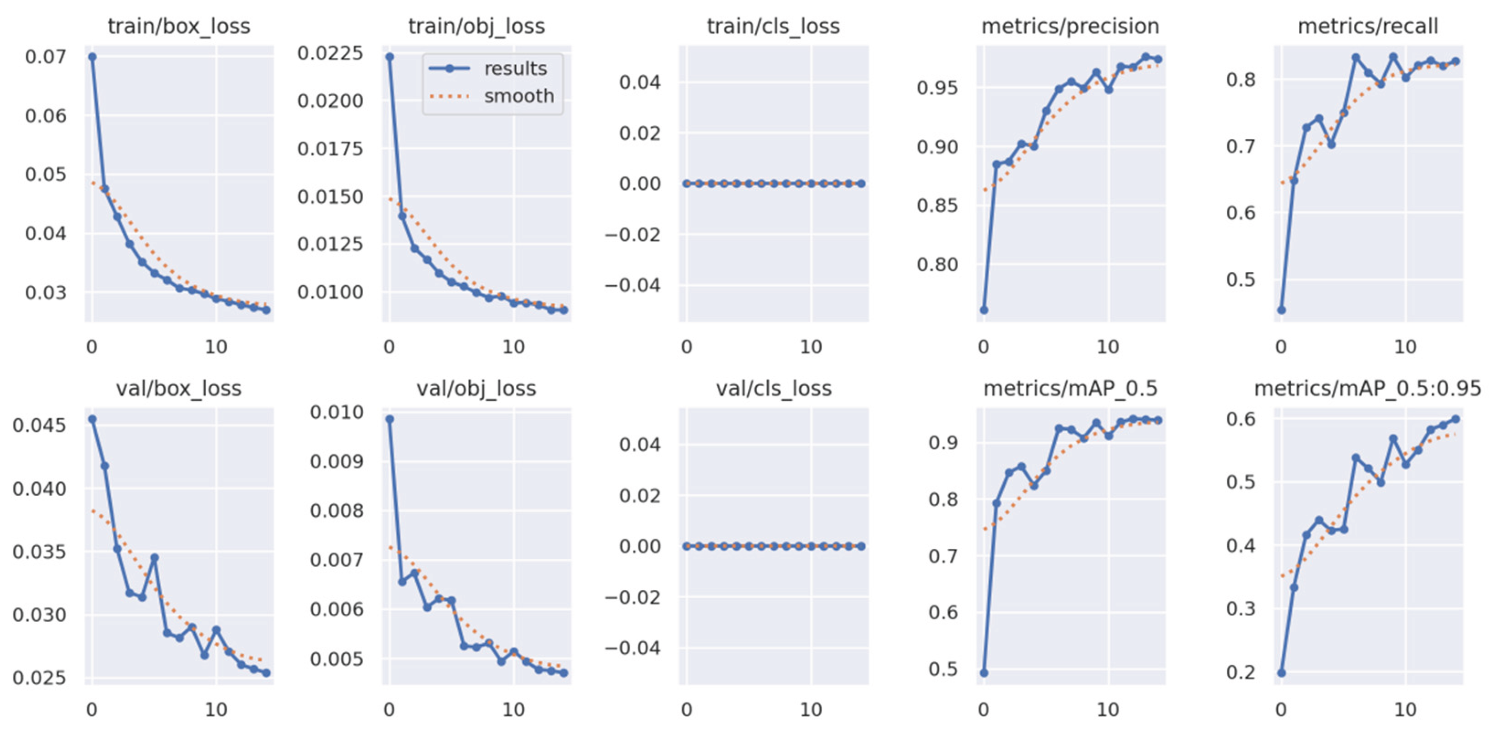
YOLOv5 was selected over newer versions such as YOLOv6, YOLOv7, or YOLOv8 for several practical reasons. First, YOLOv5 remains widely supported and actively maintained, with comprehensive documentation and community resources. Second, it is known for being lightweight and easy to deploy, which is especially valuable in rapid prototyping and real-time applications. Finally, its modular architecture and high customizability made it well-suited for adaptation to the constraints of the current project. The training results for YOLOv5 are presented in Appendix B (Figure B1, Figure B2, Figure B3, Figure B4 and Figure B5).
When comparing the training performance between YOLOv5 and the proposed SARGAS algorithm, it is evident that SARGAS achieves smoother and more stable training curves, particularly in the later epochs. In contrast, YOLOv5’s training accuracy and loss metrics show continued fluctuation, suggesting less consistent convergence.
To evaluate the performance of the proposed detection algorithm, we use standard classification metrics derived from the confusion matrix—namely, accuracy, precision, recall, and F1 score. These metrics are computed based on the number of true positives (TP), true negatives (TN), false positives (FP), and false negatives (FN), which are determined by comparing the algorithm’s outputs against hand-labeled ground truth on the same video footage.
Since the algorithm performs both object presence detection and localization, a true positive is counted when a human is correctly detected and the predicted bounding box overlaps with the ground truth by at least 50% Intersection over Union (IoU). A false negative occurs when a human is present in the frame but either no detection is made or the bounding box fails to meet the IoU threshold. A false positive is defined as a detection in which no human is present, or where the predicted bounding box does not correspond to any valid ground truth object. A true negative is recorded when no detection is made and no human is present in the scene.
Although mean Average Precision (mAP) is a widely adopted metric in object detection benchmarks—particularly those involving multi-class tasks or dense object distributions—we use confusion matrix-based metrics due to the binary, single-class nature of our task. The algorithm is specifically designed to detect and localize humans in drone-captured video. Thus, our evaluation focuses on both the detection correctness and the localization precision of a single object class. In this context, accuracy, precision, recall, and F1 score provide more interpretable and practically meaningful insights into the model's real-world performance.
Nonetheless, we acknowledge the comprehensiveness of mAP as an evaluation metric and plan to incorporate it in future work, particularly if the system is expanded to handle multi-class detection or if ranking of predictions becomes necessary. To further clarify how these metrics are computed, we provide the formal definitions below. These equations are based on standard confusion matrix terminology.
Accuracy measures the overall proportion of correct predictions—both positive and negative—across all evaluated instances and can be represented with following equation:
Precision reflects the reliability of positive predictions by quantifying how many predicted positives are actually correct and can be calculated with the following equation:
Recall measures the model's ability to detect all actual instances of the object of interest, which is particularly critical in high-risk applications such as search and rescue. It can be calculated using the following equation:
The F1 score provides a balanced harmonic mean of precision and recall, offering a single metric that accounts for both false positives and false negatives. It can be calculated with the following equation:
An example of a detection performed by the SARGAS algorithm during the first inference test is presented in Figure 6.
Following the analysis of accuracy, precision, recall, and F1 score, the full confusion matrix for each evaluated algorithm is shown in Table 2. The evaluation was conducted on video footage partially overlapping with the training set.
In addition, the corresponding performance metrics derived from the confusion matrix values are summarized in Table 3, providing an alternative view of each algorithm's detection quality.
As shown in Table 3, the YOLOv5 algorithm demonstrates higher accuracy compared to the custom SARGAS algorithm. This outcome highlights the advantage of supervised learning, particularly when the inference data closely resembles the training data. However, this performance benefit diminishes when inference is conducted on a different video sequence that bears no similarity to the training set. This effect is illustrated in Figure 7, where a randomly selected set of nine images from both evaluation tests (YOLOv5 and SARGAS) is presented to demonstrate their respective performance in practical scenarios.
The results of the inference test conducted on video footage unrelated to the training data are presented in Table 4. Although the scene is visually simple—comprising primarily of snow with minimal background clutter—this test case is designed to highlight a key limitation of fast, supervised algorithms such as YOLOv5, which may overfit to training distributions. In contrast, the test also demonstrates the generalization strengths of our custom, unsupervised algorithm under minimal-scene conditions.
The performance metrics derived from the second video and the associated prediction scores demonstrate a clear advantage of our custom algorithm over YOLOv5 when applied to previously unseen data. Unlike YOLOv5, which relies heavily on supervised learning and exhibits notable performance degradation under domain shift, our algorithm—trained in a partially unsupervised manner—learns feature patterns autonomously and generalizes more effectively. This suggests enhanced robustness in real-world scenarios where input data may deviate from the training distribution. Additionally, it is worth noting that YOLOv5 retains all predicted bounding boxes along with their confidence scores, whereas our algorithm employs a post-classification filtering step that discards all detections below a confidence threshold of 0.85, thereby reducing false positive noise.
The evaluation conducted on footage unrelated to the training data reveals significant differences in the generalization capabilities of the tested algorithms. As shown in Table 5 and the corresponding confusion matrix, the SARGAS algorithm maintains a strong balance between precision (95.58%) and recall (88.79%), achieving an F1 score of 92.06%. These results indicate that SARGAS retains robust detection performance under domain shift, with relatively few false positives (FP = 59) and a manageable number of false negatives (FN = 161) out of 1436 possible detections.
In contrast, YOLOv5—while performing well on data resembling its training distribution—struggles when applied to novel data. Its recall drops sharply to 29.04%, resulting in more than 1000 missed detections (FN = 1019), despite maintaining moderate precision. The resulting F1 score of 41.39% reflects reduced practical applicability in scenarios where the test environment diverges from training conditions.
Faster-RCNN achieves near-perfect results, with a precision of 99.7%, recall of 99.9%, and an F1 score of 99.8%, detecting nearly all objects with minimal false detections (FP = 4, FN = 1). This reflects excellent robustness and generalization, although the computational cost and longer inference time may hinder its use in time-sensitive or resource-constrained environments such as onboard drone systems.
Meanwhile, cutLER fails to detect any objects in the test footage (TP = 0, FN = 1436), revealing its limited capability in generalizing without prior domain adaptation. As an unsupervised method, it may require further tuning to be viable in real-time search and rescue operations.
In summary, although Faster-RCNN delivers the highest raw detection accuracy, the SARGAS algorithm offers a promising balance of generalization ability, precision, and computational efficiency—making it a strong candidate for deployment in dynamic, real-world environments where labeled training data may be scarce.
Surprisingly, Faster-RCNN demonstrated consistently high performance across both evaluation scenarios, while YOLOv5 showed a marked decline during inference on the second video. In contrast, the performance of the proposed SARGAS method remained stable, exhibiting only a minor drop of approximately 5% in recall despite significant changes in the input distribution.
4. Discussion
The results of this study have exceeded initial expectations, particularly given that few existing object detection systems rely on a binary classifier as their primary detection mechanism. The original intent was to enhance motion detection using traditional optical flow algorithms, such as the Lucas-Kanade or Horn-Schunck methods, in combination with background subtraction. However, these approaches proved ineffective in the context of simultaneous motion of both the camera drone and the object of interest. The application of affine transformations in this setting further exacerbated the issue, introducing distortions that undermined reliable motion differentiation.
Conversely, the Mixture of Gaussians (MOG2) background subtraction method demonstrated surprisingly robust performance. While it did not introduce additional false positives, it successfully detected objects of interest in instances where the sliding window method failed. Nevertheless, the MOG2 approach comes with a notable limitation: it performs optimally when the camera maintains a top-down perspective. Detection quality degrades substantially when the camera captures side views, and performance is poorest in front or rear views where motion is minimal and the subject size exceeds the sliding window capacity. Under such conditions, both detection branches face challenges in reliably identifying human subjects.
When benchmarked against a supervised object detector such as YOLOv5, the SARGAS system does underperform in terms of overall detection metrics. However, this comparison must be contextualized: YOLOv5 benefits from extensive supervised training and large annotated datasets, while SARGAS relies on an unsupervised learning paradigm and minimal manual input. Given the scarcity of existing object detectors that train effectively on unlabeled data, the development and deployment of SARGAS represent a meaningful contribution to the field.
The observed rate of false positives highlights an area requiring further investigation. Future work will focus on refining the post-processing pipeline, enhancing classification accuracy, and improving overall reliability. Despite its current limitations, SARGAS demonstrates promising adaptability and potential for improvement. With further optimization and access to more powerful computational resources, we strongly believe that unsupervised CNN-based object detectors may eventually rival or even surpass their supervised counterparts in both flexibility and performance.
5. Conclusions
The primary objective of this study has been successfully achieved: the development of a novel object detection pipeline centered around a binary classifier. While the overall system is still in an early phase and leaves room for improvement, the foundational architecture has been established, demonstrating promising potential for further refinement and application.
In challenging conditions—where the object of interest could easily blend with its surroundings—the proposed SARGAS algorithm achieved a recall rate of 92.42%, with moderate accuracy and precision of 65.00% and 68.16%, respectively. These results are particularly noteworthy given the limited use of supervised data and the reliance on unsupervised learning techniques.
Moreover, when tested on previously unseen video footage, the SARGAS algorithm significantly outperformed the YOLOv5 model. It achieved an accuracy of 85.28% compared to YOLOv5’s 26.10%, with a notable 23.56% higher precision. This highlights the algorithm’s superior generalization capabilities and its potential for deployment in real-world scenarios where training data may not reflect operational environments.
Although further optimization is necessary—particularly in reducing false positives and improving robustness under diverse viewing conditions—the current results confirm the viability of the proposed approach and lay a strong foundation for future advancements.
Author Contributions
Conceptualization, G.V. and I.S.; methodology, G.V.; software, G.V.; validation, I.S., formal analysis, G.V.; investigation, G.V.; resources, G.V.; data curation, G.V.; writing—original draft preparation, G.V.; writing—review and editing, I.D.; visualization, G.V.; supervision, I.D.; project administration, I.D.; funding acquisition, I.D. All authors have read and agreed to the published version of the manuscript.
Funding
This research received no external funding.
Data Availability Statement
The datasets presented in this article are not readily available because the data are part of an ongoing study. Requests to access the datasets should be directed to the corresponding author.
Acknowledgments
Main support and materials were obtained from Antanas Gustaitis’ Aviation Institute, Vilnius Gediminas Technical University.
Conflicts of Interest
The authors declare no conflicts of interest.
Appendix A
Figure A1.
Relu accuracy and loss over epochs subset 0.
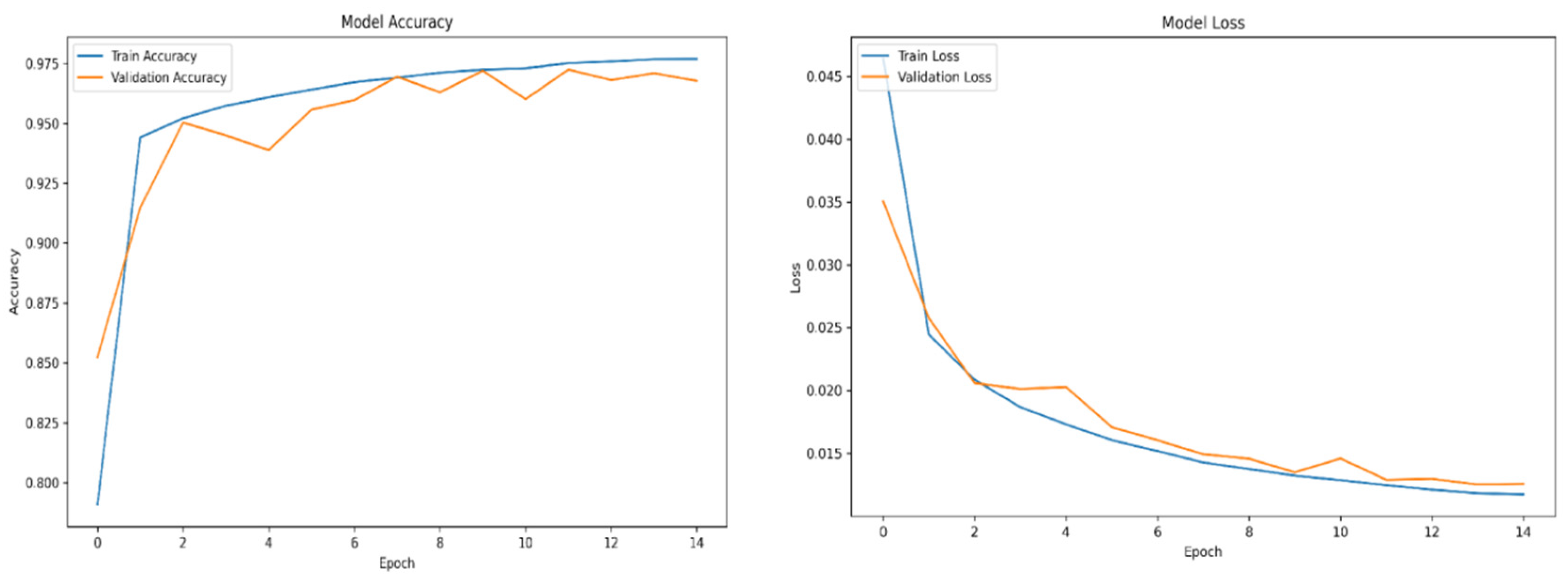
Figure A2.
Relu accuracy and loss over epochs subset 1.
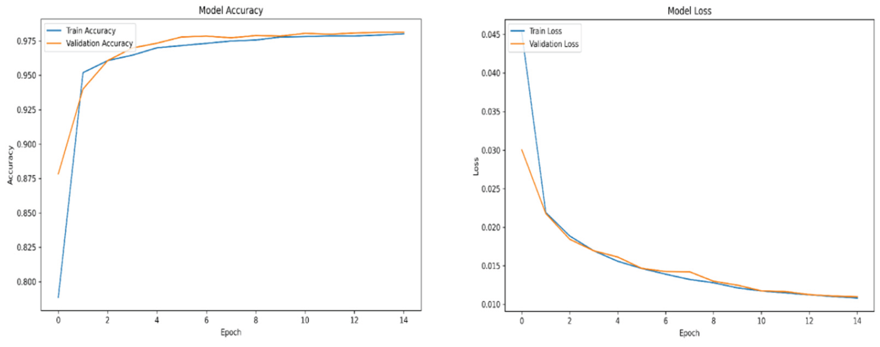
Figure A3.
Relu accuracy and loss over epochs subset 2.
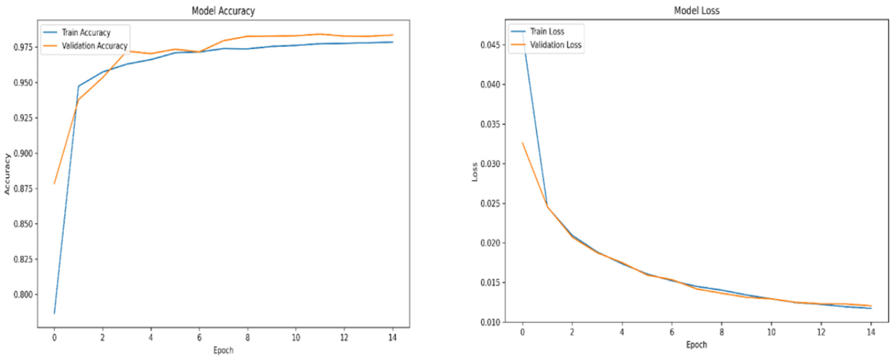
Figure A4.
Relu accuracy and loss over epochs subset 3.
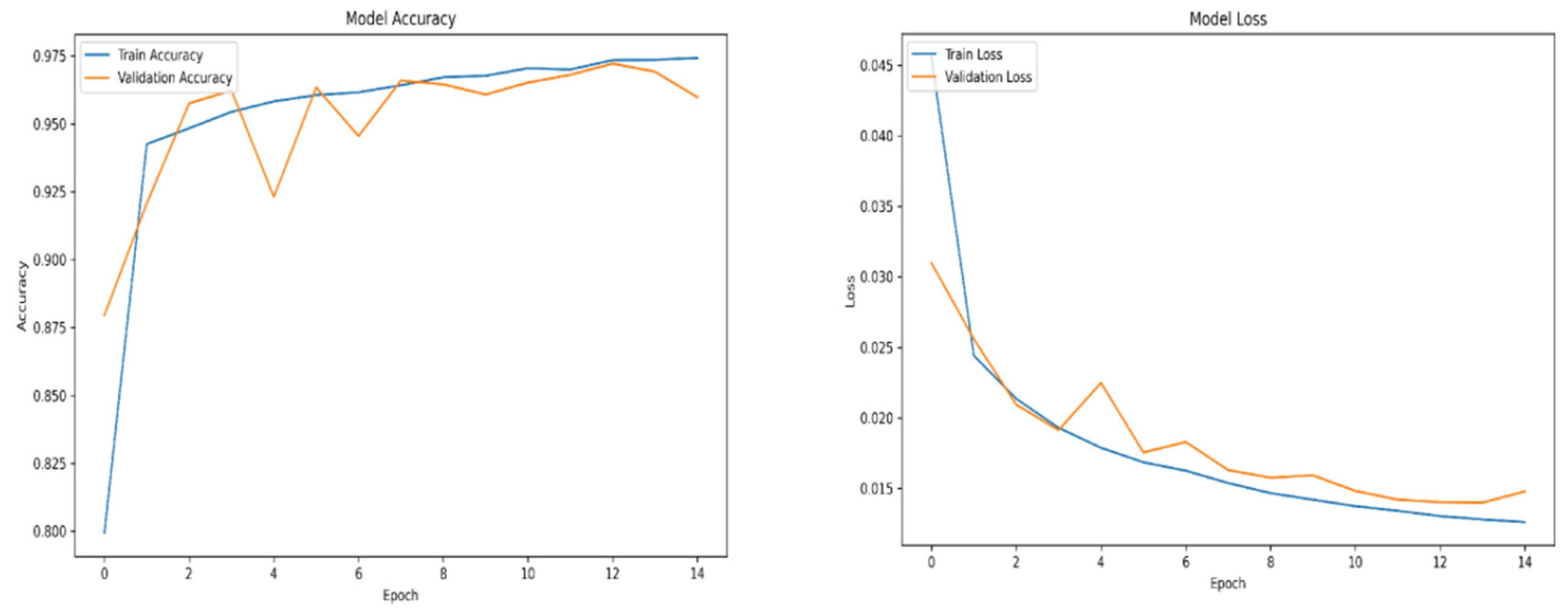
Figure A5.
Relu accuracy and loss over epochs subset 4.
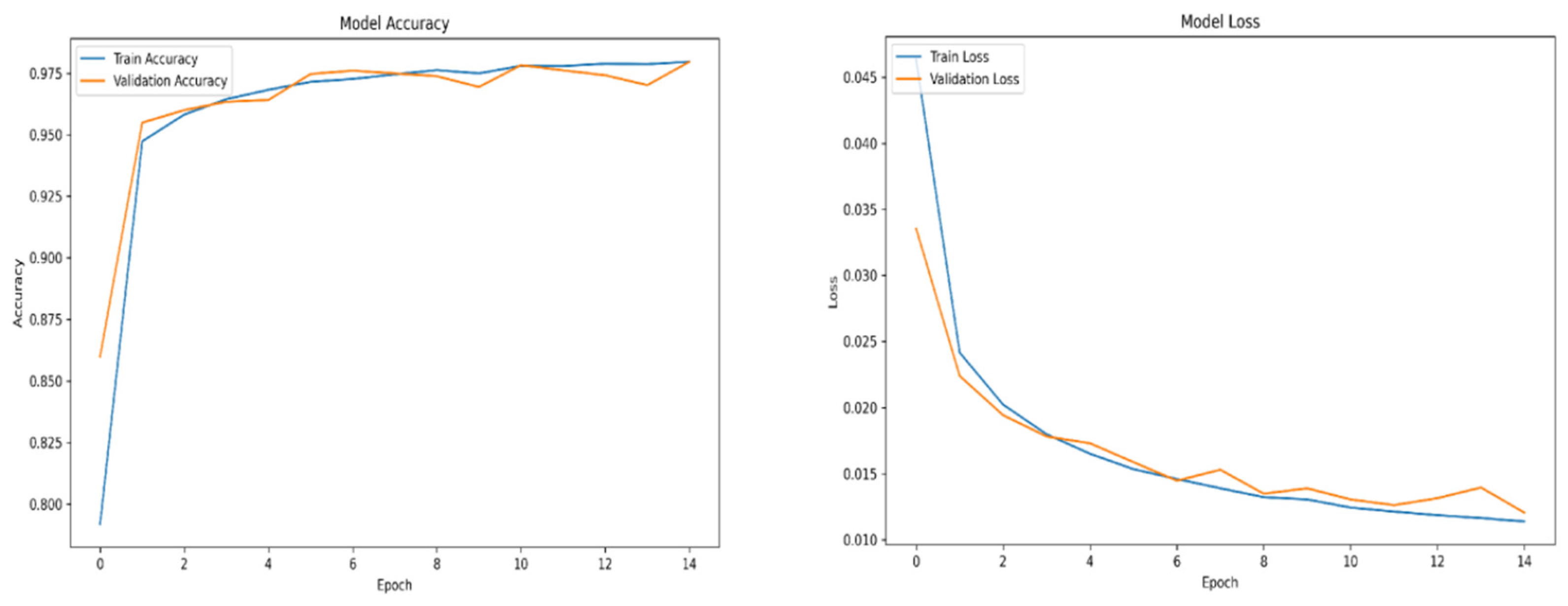
Figure A6.
Swish accuracy and loss over epochs subset 0.
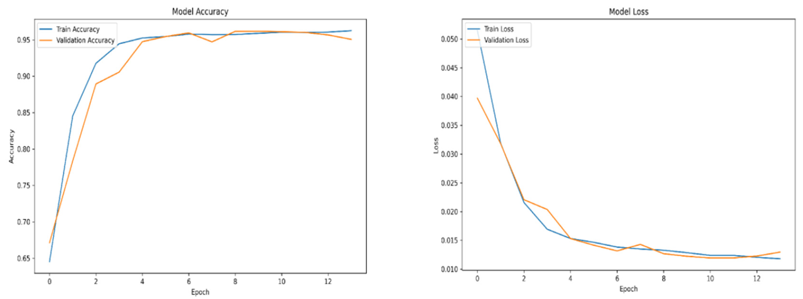
Figure A7.
Swish accuracy and loss over epochs subset 1.
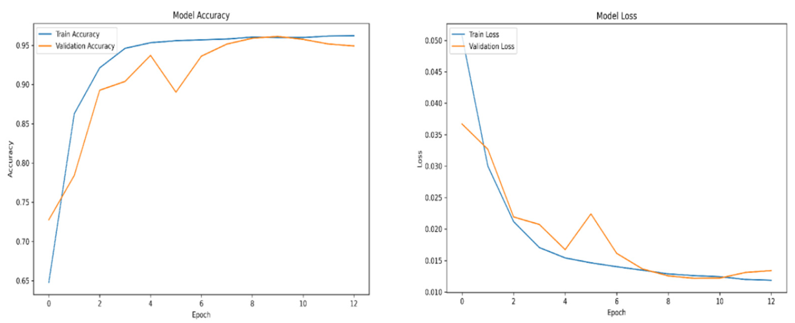
Figure A8.
Swish accuracy and loss over epochs subset 2.
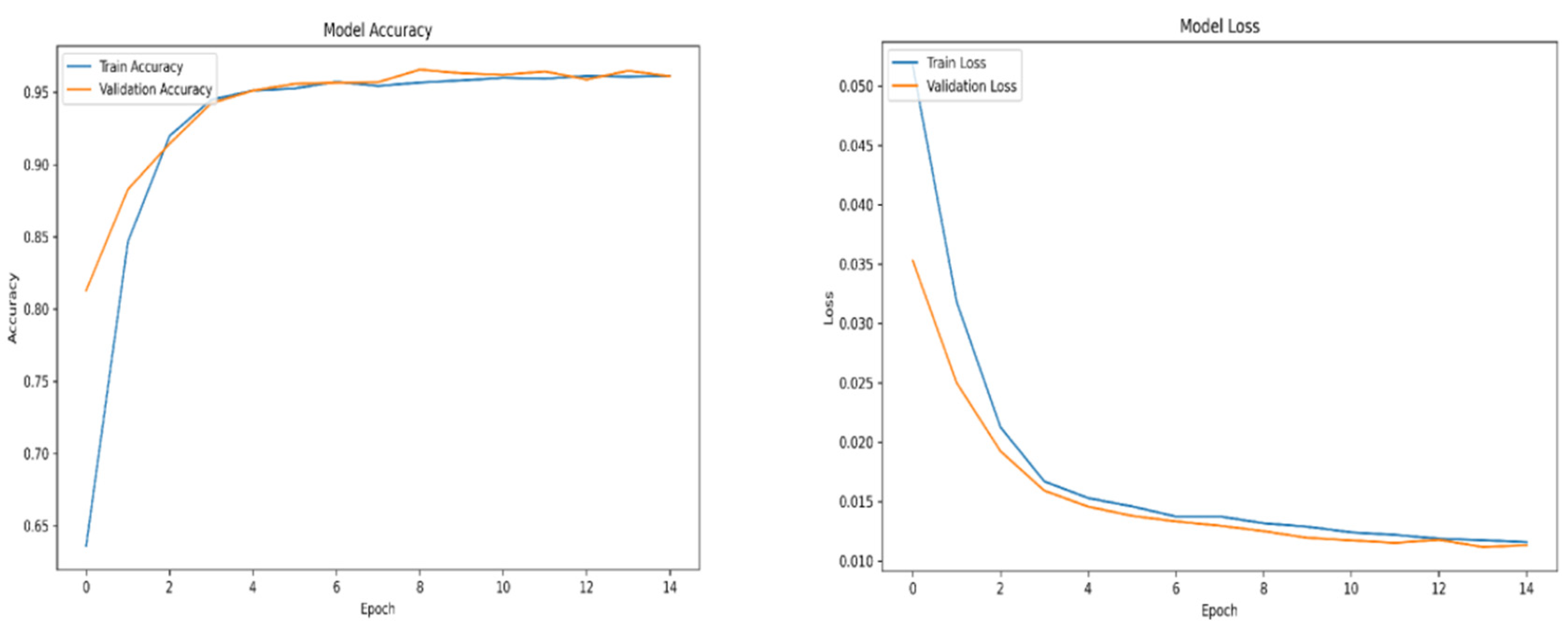
Figure A9.
swish accuracy and loss over epochs subset 3.
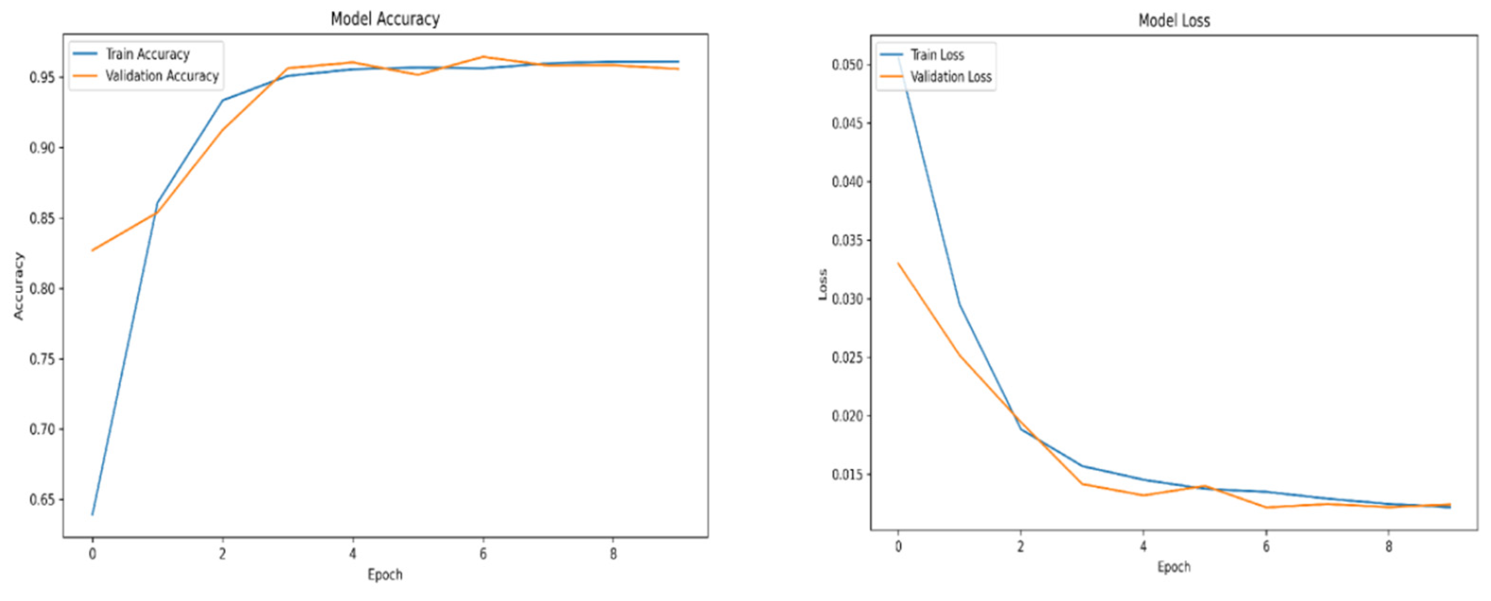
Figure A10.
Swish accuracy and loss over epochs subset 4.
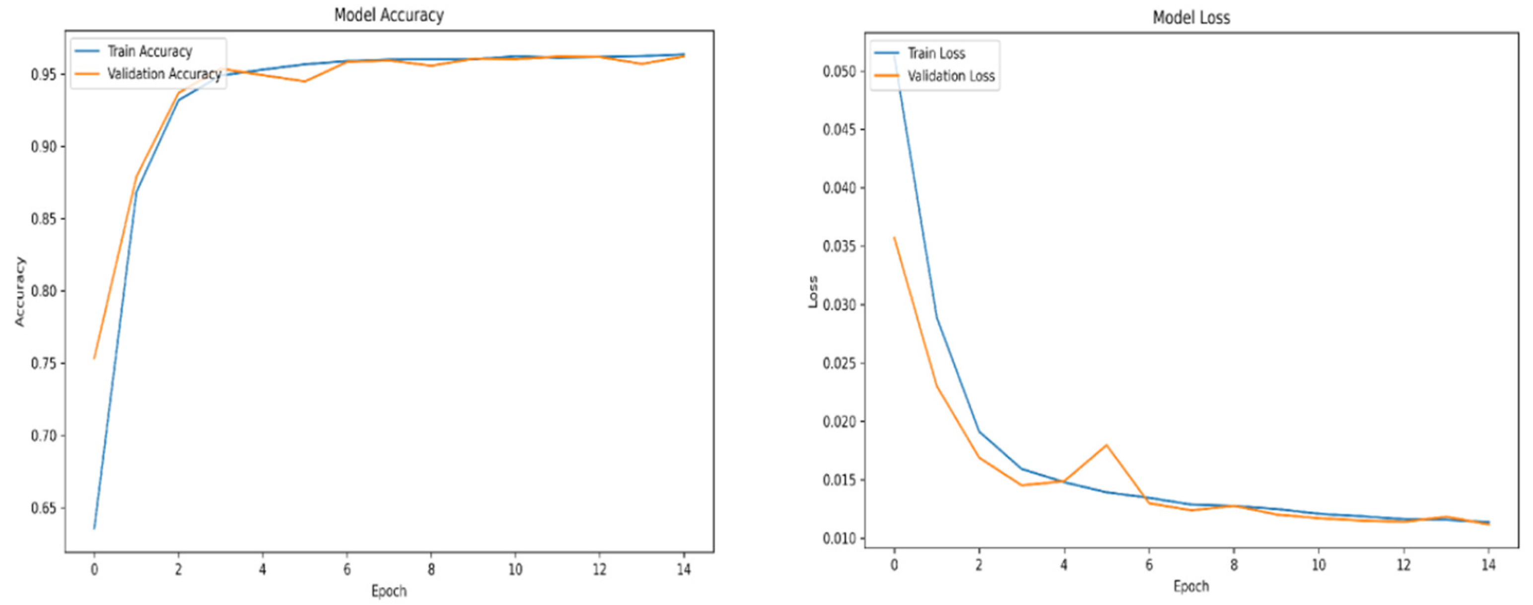
Appendix B
Figure B1.
Yolov5 training over epochs subset.
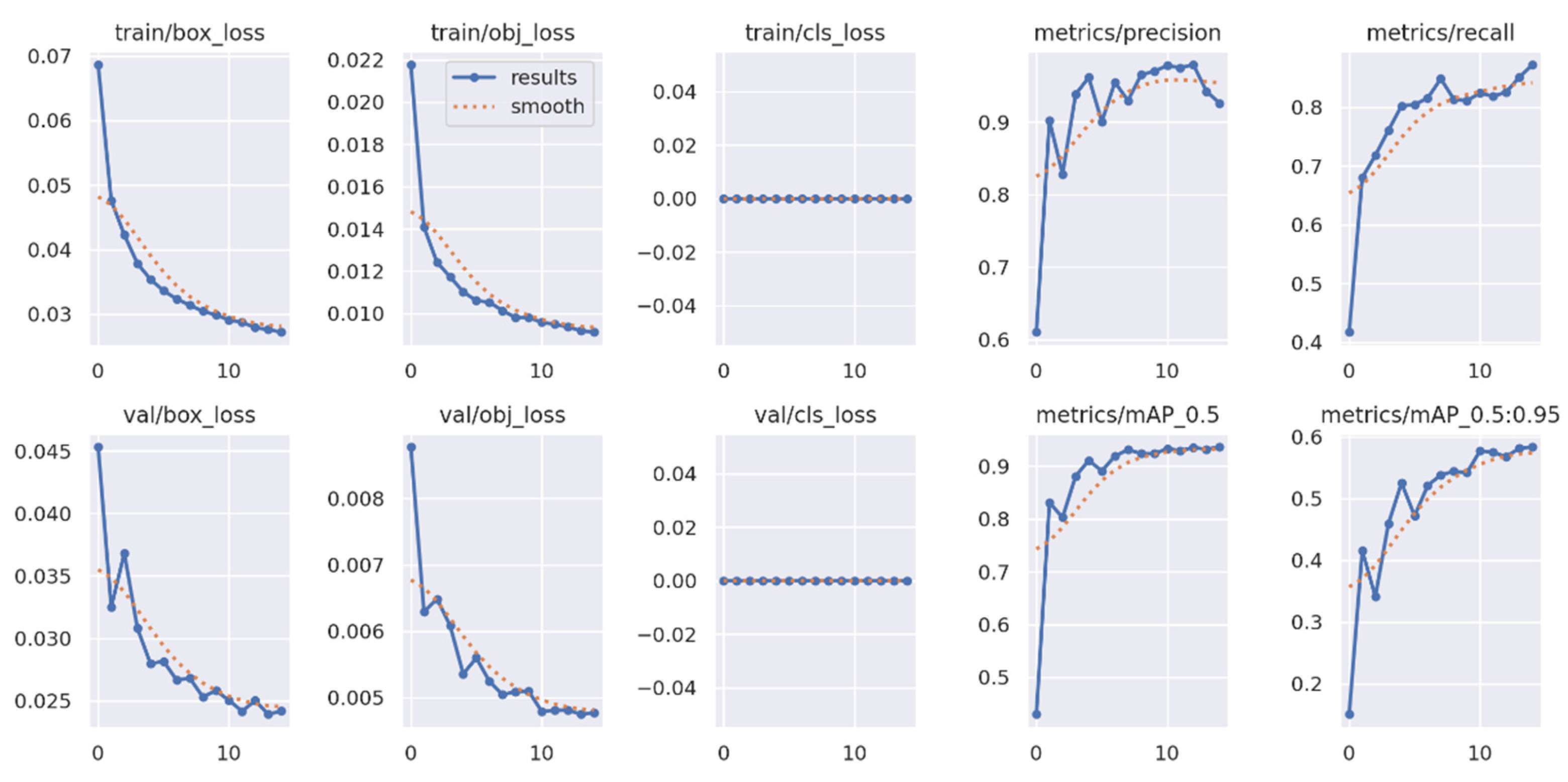
Figure B2.
Yolov5 training over epochs subset 1.
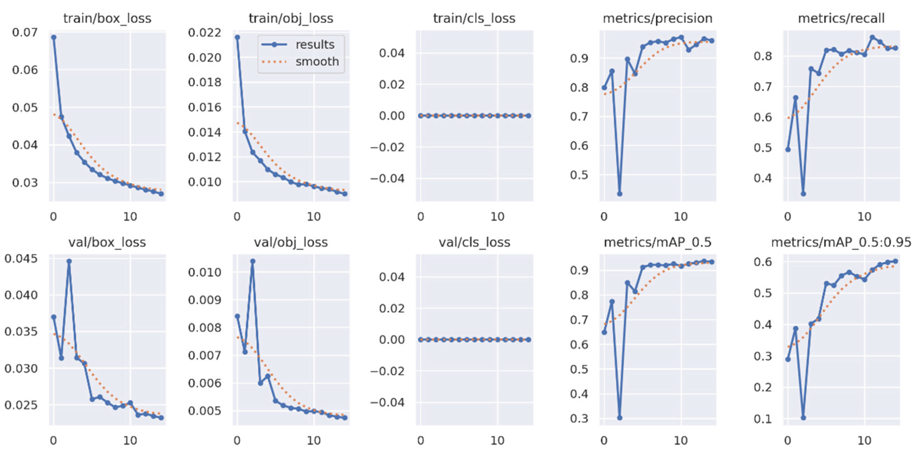
Figure B3.
Yolov5 training over epochs subset 2.
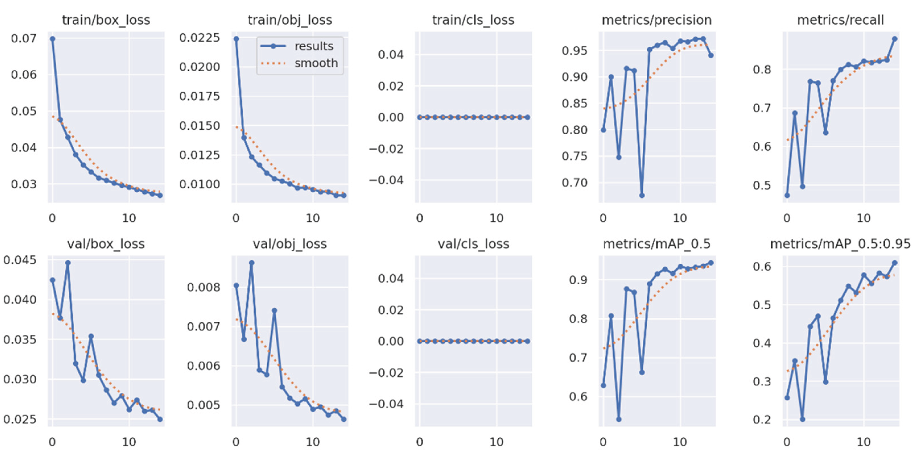
Figure B4.
Yolov5 training over epochs subset.
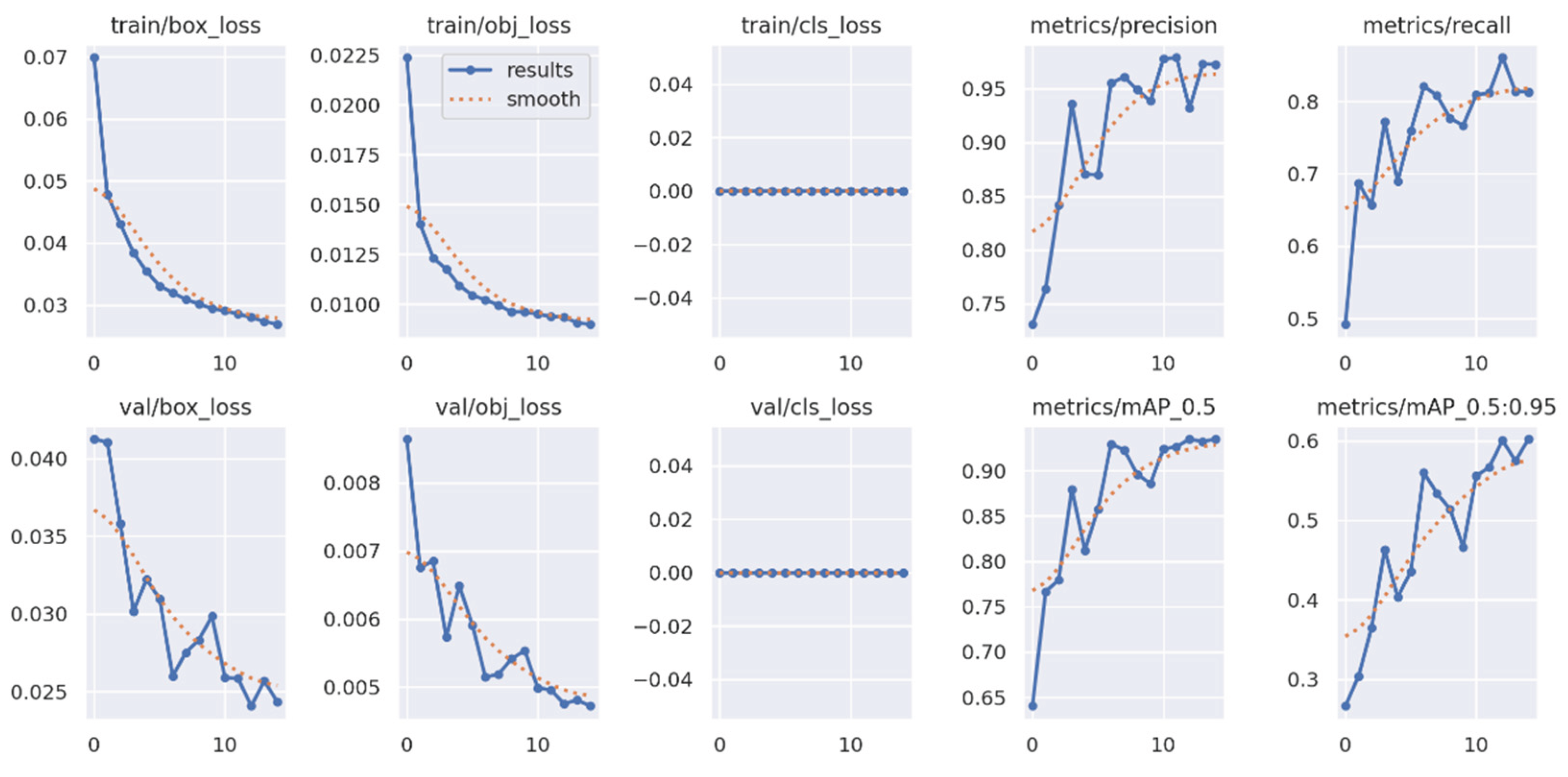
Figure B5.
Yolov5 training over epochs subset 4.
References
- Turgut and T. Turgut, “A study on ‘rescuer’ drowning and multiple drowning incidents,” J Safety Res, vol. 43, no. 2, pp. 129–132, Apr. 2012. [CrossRef]
- L. T. I. Penman, “New Light on the Survivors of the Vergulde Draak, a VOC Ship Wrecked on the Australian Coast (1656),” Mar Mirror, vol. 108, no. 2, pp. 149–158, 2022. [CrossRef]
- Y. Karaca et al., “The potential use of unmanned aircraft systems (drones) in mountain search and rescue operations,” American Journal of Emergency Medicine, vol. 36, no. 4, pp. 583–588, Apr. 2018. [CrossRef]
- R. Zhang et al., “Automatic detection of earthquake-damaged buildings by integrating UAV oblique photography and infrared thermal imaging,” Remote Sens (Basel), vol. 12, no. 16, Aug. 2020. [CrossRef]
- E. Yalcin, G. A. Ciftcioglu, and B. H. Guzel, “Human Factors Analysis by Classifying Chemical Accidents into Operations,” Sustainability (Switzerland), vol. 15, no. 10, May 2023. [CrossRef]
- D. H. Waskito et al., “Analysing the Impact of Human Error on the Severity of Truck Accidents through HFACS and Bayesian Network Models,” Safety, vol. 10, no. 1, Mar. 2024. [CrossRef]
- L. Kasyk, A. E. Wolnowska, K. Pleskacz, and T. Kapuściński, “The Analysis of Social and Situational Systems as Components of Human Errors Resulting in Navigational Accidents,” Applied Sciences (Switzerland), vol. 13, no. 11, Jun. 2023. [CrossRef]
- M. K. Jalehi and B. M. Albaker, “Highly accurate multiclass classification of respiratory system diseases from chest radiography images using deep transfer learning technique,” Biomed Signal Process Control, vol. 84, Jul. 2023. [CrossRef]
- N. Huda and K. R. Ku-Mahamud, “CNN-Based Image Segmentation Approach in Brain Tumor Classification: A Review,” in The 8th Mechanical Engineering, Science and Technology International Conference, Basel Switzerland: MDPI, Feb. 2025, p. 66. [CrossRef]
- S. Hwang, J. Park, N. Kim, Y. Choi, and I. S. Kweon, “Multispectral Pedestrian Detection: Benchmark Dataset and Baseline.” [Online]. Available: http://rcv.kaist.ac.kr/multispectral-pedestrian/.
- B. Schofield, N. Iversen, and E. Ebeid, “Autonomous power line detection and tracking system using UAVs,” Microprocess Microsyst, vol. 94, Oct. 2022. [CrossRef]
- 12. M. C. Tatum and J. Liu, “Unmanned Aircraft System Applications in Construction,” in Procedia Engineering, Elsevier Ltd, 2017, pp. 167–175. [CrossRef]
- M. B. Khan, S. Tamkin, J. Ara, M. Alam, and H. Bhuiyan, “CropsDisNet: An AI-Based Platform for Disease Detection and Advancing On-Farm Privacy Solutions,” Data (Basel), vol. 10, no. 2, Feb. 2025. [CrossRef]
- L. Hui, A. Ibrahim, and R. Hindi, “Computer Vision-Based Concrete Crack Identification Using MobileNetV2 Neural Network and Adaptive Thresholding,” Infrastructures (Basel), vol. 10, no. 2, Feb. 2025. [CrossRef]
- T. M. Mitchell, Machine Learning, 1st ed. USA: McGraw-Hill, Inc., 1997.
- E. Alpaydin, Introduction to Machine Learning (Adaptive Computation and Machine Learning). The MIT Press, 2004.
- H. A. Simon and A. Newell, “Heuristic Problem Solving: The Next Advance in Operations Research,” Oper Res, vol. 6, pp. 1–10, 1958, [Online]. Available: https://api.semanticscholar.org/CorpusID:62443902.
- J. Heaton, “Ian Goodfellow, Yoshua Bengio, and Aaron Courville: Deep learning: The MIT Press, 2016, 800 pp, ISBN: 0262035618,” Genet Program Evolvable Mach, vol. 19, Apr. 2017. [CrossRef]
- Krizhevsky, I. Sutskever, and G. Hinton, “ImageNet Classification with Deep Convolutional Neural Networks,” Neural Information Processing Systems, vol. 25, Apr. 2012. [CrossRef]
- Szegedy et al., “Going deeper with convolutions,” in 2015 IEEE Conference on Computer Vision and Pattern Recognition (CVPR), 2015, pp. 1–9. [CrossRef]
- S. Hochreiter and J. Schmidhuber, “Long Short-Term Memory,” Neural Comput, vol. 9, pp. 1735–1780, Apr. 1997. [CrossRef]
- K. He, X. Zhang, S. Ren, and J. Sun, “Deep Residual Learning for Image Recognition,” in 2016 IEEE Conference on Computer Vision and Pattern Recognition (CVPR), 2016, pp. 770–778. [CrossRef]
- K. Simonyan and A. Zisserman, “Very Deep Convolutional Networks for Large-Scale Image Recognition,” CoRR, vol. abs/1409.1556, 2014, [Online]. Available: https://api.semanticscholar.org/CorpusID:14124313.
- R. Girshick, J. Donahue, T. Darrell, and J. Malik, “Rich Feature Hierarchies for Accurate Object Detection and Semantic Segmentation,” in 2014 IEEE Conference on Computer Vision and Pattern Recognition, 2014, pp. 580–587. [CrossRef]
- R. Girshick, “Fast R-CNN,” in 2015 IEEE International Conference on Computer Vision (ICCV), 2015, pp. 1440–1448. [CrossRef]
- S. Ren, K. He, R. Girshick, and J. Sun, “Faster R-CNN: Towards Real-Time Object Detection with Region Proposal Networks,” IEEE Trans Pattern Anal Mach Intell, vol. 39, no. 6, pp. 1137–1149, 2017. [CrossRef]
- J. Redmon, S. Divvala, R. Girshick, and A. Farhadi, “You Only Look Once: Unified, Real-Time Object Detection,” in 2016 IEEE Conference on Computer Vision and Pattern Recognition (CVPR), 2016, pp. 779–788. [CrossRef]
- D. and E. D. and S. C. and R. S. and F. C.-Y. and B. A. C. Liu Wei and Anguelov, “SSD: Single Shot MultiBox Detector,” in Computer Vision – ECCV 2016, J. and S. N. and W. M. Leibe Bastian and Matas, Ed., Cham: Springer International Publishing, 2016, pp. 21–37.
- Y. Chen, L. Li, W. Li, Q. Guo, Z. Du, and Z. Xu, “Chapter 1 - Introduction,” in AI Computing Systems, Y. Chen, L. Li, W. Li, Q. Guo, Z. Du, and Z. Xu, Eds., Morgan Kaufmann, 2024, pp. 1–16. [CrossRef]
- Y. Zhang, Y. Yin, and Z. Shao, “An Enhanced Target Detection Algorithm for Maritime Search and Rescue Based on Aerial Images,” Remote Sens (Basel), vol. 15, no. 19, Oct. 2023. [CrossRef]
- M. B. Bejiga, A. Zeggada, A. Nouffidj, and F. Melgani, “A convolutional neural network approach for assisting avalanche search and rescue operations with UAV imagery,” Remote Sens (Basel), vol. 9, no. 2, 2017. [CrossRef]
- S. Gotovac, D. Zelenika, Ž. Marušić, and D. Božić-štulić, “Visual-based person detection for search-and-rescue with uas: Humans vs. machine learning algorithm,” Remote Sens (Basel), vol. 12, no. 20, pp. 1–25, Oct. 2020. [CrossRef]
- 33. R. Jain and H.-H. Nagel, “On the Analysis of Accumulative Difference Pictures from Image Sequences of Real World Scenes,” IEEE Trans Pattern Anal Mach Intell, vol. PAMI-1, no. 2, pp. 206–214, 1979. [CrossRef]
- R. Wren, A. Azarbayejani, T. Darrell, and A. P. Pentland, “Pfinder: real-time tracking of the human body,” IEEE Trans Pattern Anal Mach Intell, vol. 19, no. 7, pp. 780–785, 1997. [CrossRef]
- Stauffer and W. E. L. Grimson, “Adaptive background mixture models for real-time tracking,” in Proceedings. 1999 IEEE Computer Society Conference on Computer Vision and Pattern Recognition (Cat. No PR00149), 1999, pp. 246-252 Vol. 2. [CrossRef]
- B. K. P. Horn and B. G. Schunck, “Determining optical flow,” Artif Intell, vol. 17, no. 1–3, pp. 185–203, Aug. 1981. [CrossRef]
- B. D. Lucas and T. Kanade, “An Iterative Image Registration Technique with an Application to Stereo Vision,” in International Joint Conference on Artificial Intelligence, 1981. [Online]. Available: https://api.semanticscholar.org/CorpusID:2121536.
- * Broyles, C. * Hayner, and K. Leung, “WiSARD: A Labeled Visual and Thermal Image Dataset for Wilderness Search and Rescue,” in IEEE/RSJ Int. Conf. on Intelligent Robots & Systems, 2022.
- G. Csönde, Y. Sekimoto, and T. Kashiyama, “Online real-time pedestrian tracking from medium altitude aerial footage with camera motion cancellation,” Computer Vision and Image Understanding, vol. 217, Mar. 2022. [CrossRef]
- M. Tagliasacchi, “A genetic algorithm for optical flow estimation,” Image Vis Comput, vol. 25, no. 2, pp. 141–147, 2007. [CrossRef]
- J. Ding, Z. Zhang, X. Yu, X. Zhao, and Z. Yan, “A Novel Moving Object Detection Algorithm Based on Robust Image Feature Threshold Segmentation with Improved Optical Flow Estimation,” Applied Sciences (Switzerland), vol. 13, no. 8, Apr. 2023. [CrossRef]
Figure 1.
CNN Architecture.
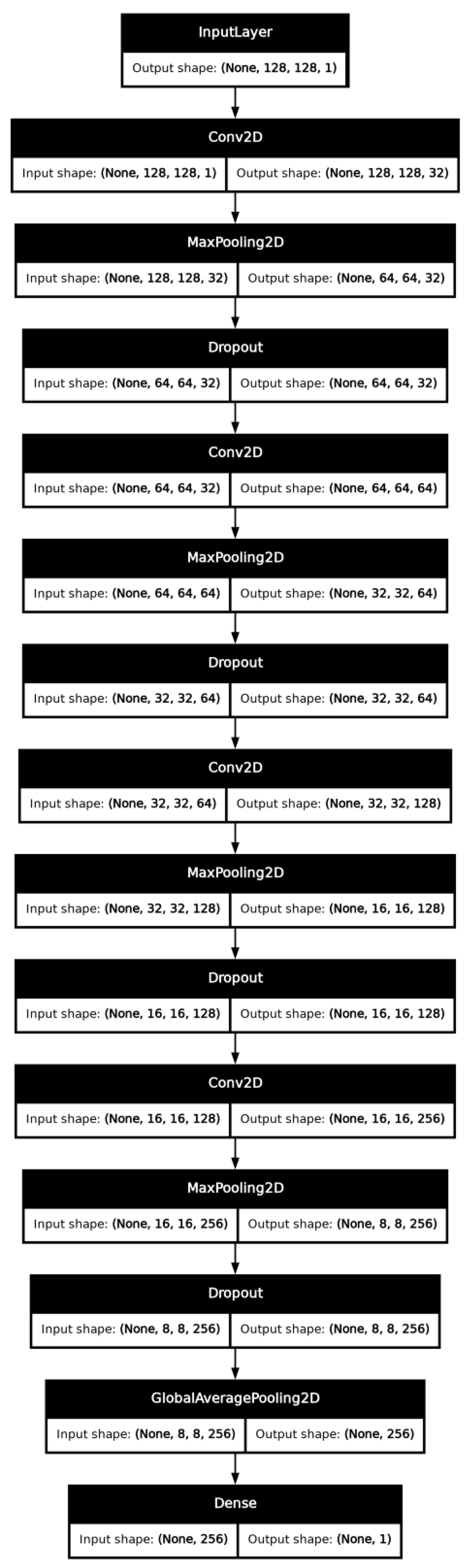
Figure 2.
Swish activation function graph example.
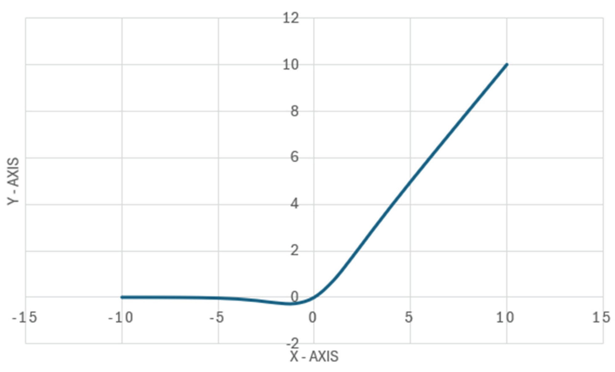
Figure 3.
Relu activation function graph example.
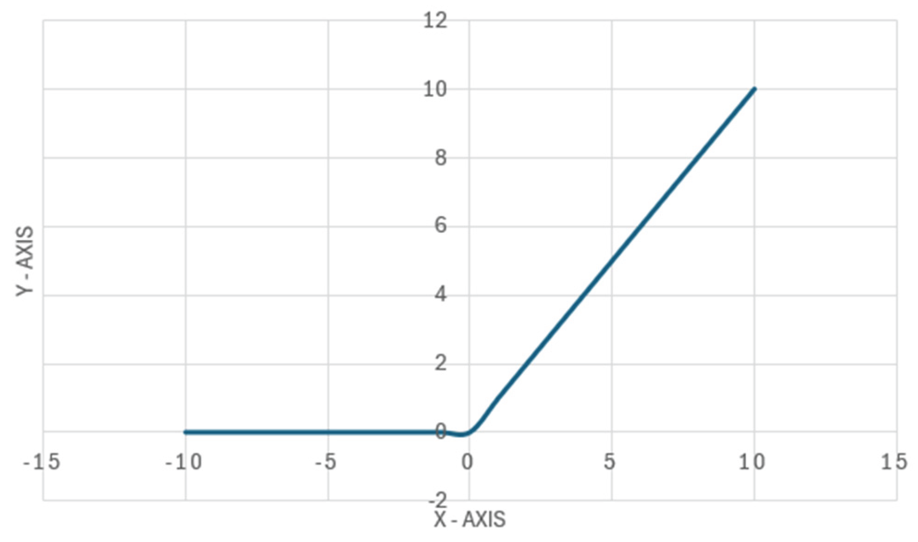
Figure 4.
Classifer structure.

Figure 5.
SARGAS Pipeline structure.
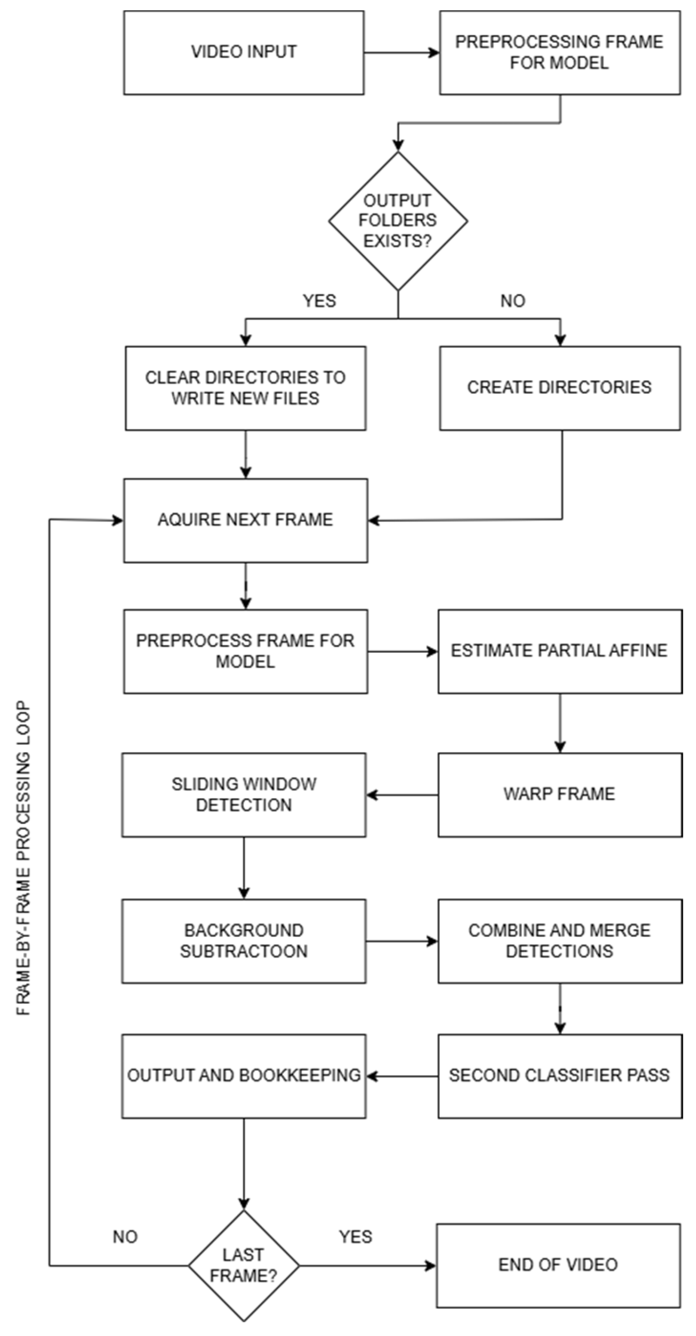
Figure 6.
First inference test example.
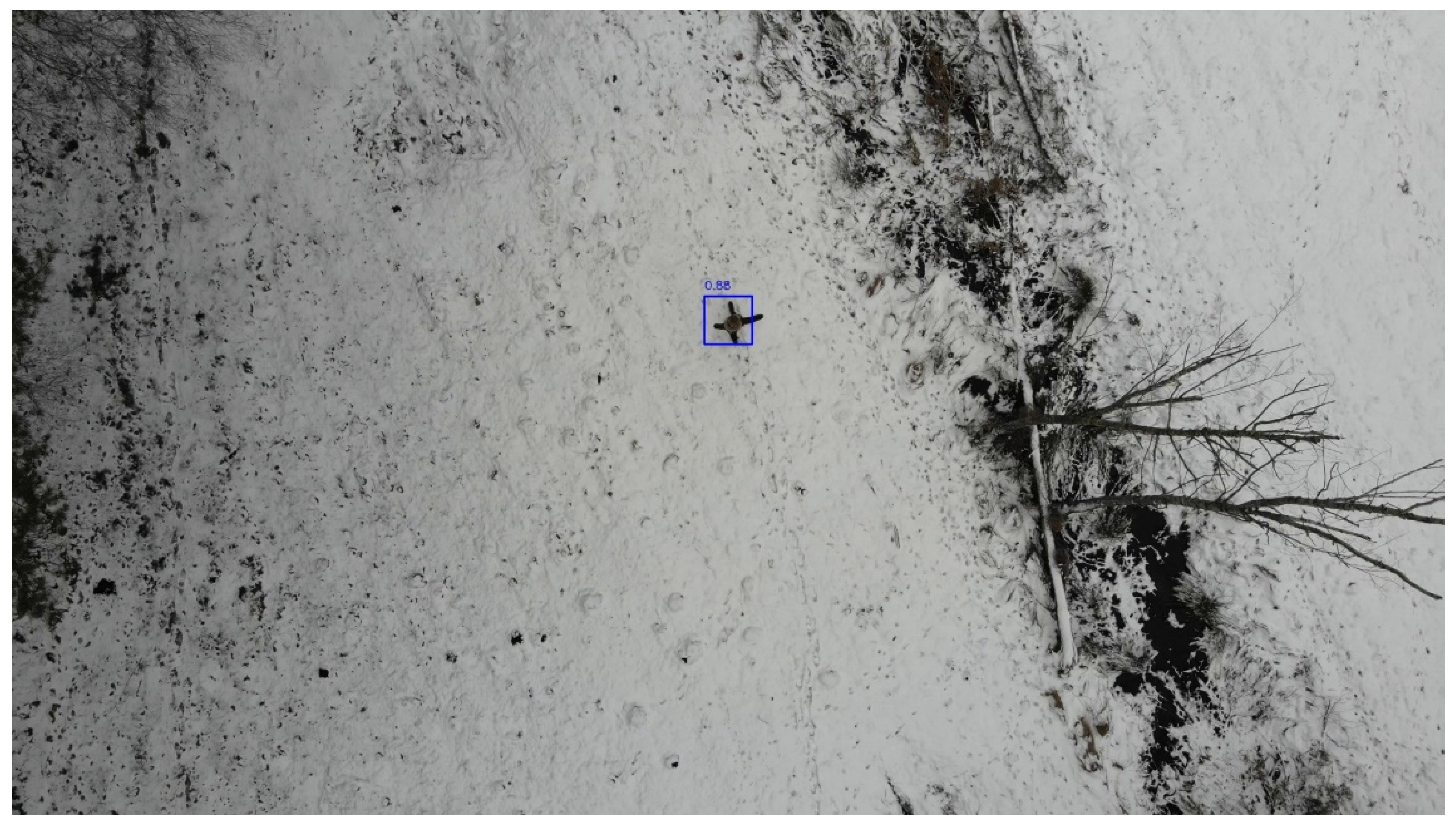
Figure 7.
YOLOv5 (left) and SARGAS (right) performance check on second video.
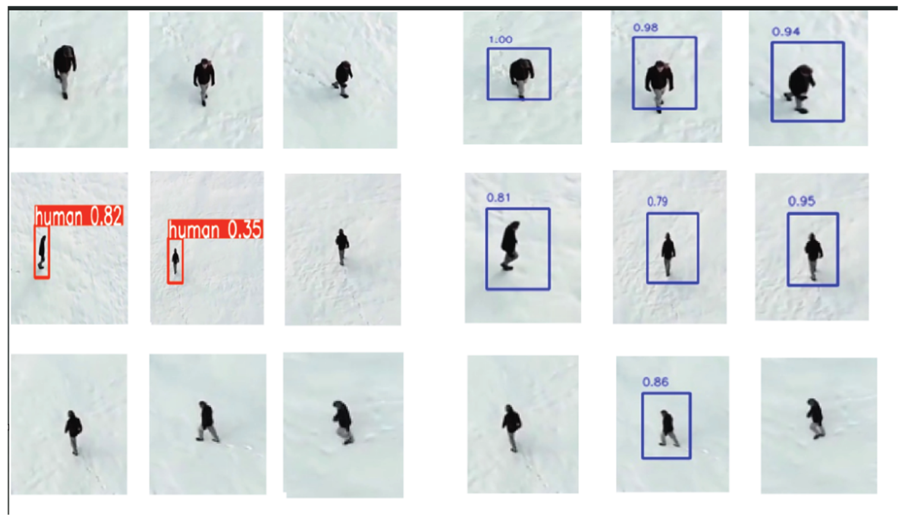
Table 2.
Algorithm performance check on similar to training data video.
| Algorithm | True Positives (TP) | False Positives (FP) | False Negatives (FN) | True Negatives (TN) |
|---|---|---|---|---|
| SARGAS | 1314 | 614 | 108 | 16 |
| YOLOv5 | 1362 | 54 | 60 | 16 |
| Faster-RCNN | 1373 | 203 | 49 | 16 |
| cutLER | 0 | 0 | 1422 | 16 |
Table 3.
Algorithm performance check on similar to training data video.
| Algorithm | Accuracy | Precision | Recall | F1 Score |
|---|---|---|---|---|
| SARGAS | 65 % | 68.16 % | 92.42 % | 78.43 % |
| YOLOv5 | 92.4 % | 96.19 % | 95.8 % | 96 % |
| Faster-RCNN | 86.95 % | 87.14 % | 96.58 % | 92.94 % |
| cutLER | 1.11 % | 0 % | 0 % | 0 % |
Table 4.
Algorithm performance check on unrelated to training data video.
| Algorithm | True Positives (TP) | False Positives (FP) | False Negatives (FN) | True Negatives (TN) |
|---|---|---|---|---|
| SARGAS | 1275 | 59 | 161 | 0 |
| YOLOv5 | 417 | 162 | 1019 | 0 |
| Faster-RCNN | 1435 | 4 | 1 | 0 |
| cutLER | 0 | 0 | 1436 | 0 |
Table 5.
Algorithm performance check on unrelated to training data video.
| Algorithm | Accuracy | Precision | Recall | F1 Score |
|---|---|---|---|---|
| SARGAS | 85.28 % | 95.58 % | 88.79 % | 92.06 % |
| YOLOv5 | 26.1 % | 72.02 % | 29.04 % | 41.39 % |
| Faster-RCNN | 99.6 % | 99.7 % | 99.9 % | 99.8 % |
| cutLER | 0 % | 0 % | 0 % | 0 % |
Disclaimer/Publisher’s Note: The statements, opinions and data contained in all publications are solely those of the individual author(s) and contributor(s) and not of MDPI and/or the editor(s). MDPI and/or the editor(s) disclaim responsibility for any injury to people or property resulting from any ideas, methods, instructions or products referred to in the content. |
© 2025 by the authors. Licensee MDPI, Basel, Switzerland. This article is an open access article distributed under the terms and conditions of the Creative Commons Attribution (CC BY) license (http://creativecommons.org/licenses/by/4.0/).
Copyright: This open access article is published under a Creative Commons CC BY 4.0 license, which permit the free download, distribution, and reuse, provided that the author and preprint are cited in any reuse.


